Multi-Dimensional mSUGRA Likelihood Maps

Abstract

We calculate the likelihood map in the full 7 dimensional parameter space of the minimal supersymmetric standard model (MSSM) assuming universal boundary conditions on the supersymmetry breaking terms. Simultaneous variations of $m_{0}$, $A_{0}$, $M_{1/2}$, $\tan\beta$, $m_{t}$, $m_{b}$ and $\alpha_{s}(M_{Z})$ are applied using a Markov chain Monte Carlo algorithm. We use measurements of $b\rightarrow s\gamma$, $(g-2)_{\mu}$ and $\Omega_{DM}h^{2}$ in order to constrain the model. We present likelihood distributions for some of the sparticle masses, for the branching ratio of $B_{s}^{0}\rightarrow\mu^{+}\mu^{-}$ and for $m_{\tilde{\tau}}-m_{\chi_{1}^{0}}$. An upper limit of 2$\times 10^{-8}$ on this branching ratio might be achieved at the Tevatron, and would rule out 29$\%$ of the currently allowed likelihood. If one allows for non thermal-neutralino components of dark matter, this fraction becomes 35$\%$. The mass ordering allows the important cascade decay ${\tilde{q}}_{L}\rightarrow{\chi_{2}^{0}}\rightarrow{\tilde{l}}_{R}\rightarrow{\chi_{1}^{0}}$ with a likelihood of 24$\pm 4\%$. The stop coannihilation region is highly disfavoured, whereas the light Higgs region is marginally disfavoured.

I Introduction

Weak-scale supersymmetry provides a well-documented solution to the technical hierarchy problem Martin:1997ns , which is particularly difficult to solve in a perturbatively calculable model. Specialising to a minimal extension of the Standard Model, the MSSM, one can provide a weakly interacting massive particle dark matter candidate, provided $R-$parity is respected by the model. Examples of dark matter candidates are the gravitino Ellis:2003dn ; Roszkowski:2004jd , the axino Covi:2004rb and the lightest neutralino Ellis:1983ew , the subject of much recent investigation Baer:2002gm ; Ellis:2003cw ; Battaglia:2003ab ; Ellis:2003si ; Gomez:2004ek ; Ellis:2004tc . The general MSSM is rather complicated due to the large number of free parameters in the supersymmetric (SUSY) breaking sector. However, the observed rareness of flavour changing neutral currents (FCNCs) suggests that the vast majority of parameter space for general SUSY breaking terms is ruled out. Particular patterns of SUSY breaking parameters can postdict small enough FCNCs: for instance flavour universality. One highly studied subset of such terms is that of mSUGRA, often called the Constrained Minimal Supersymmetric Standard Model (CMSSM). In mSUGRA, at some high energy scale (typically taken to be the scale of unification of electroweak gauge couplings), all of the SUSY breaking scalar mass terms are assumed to be equal to $m_{0}$, the scalar trilinear terms are set to $A_{0}$ and the gaugino masses are set equal ($M_{1/2}$). These are indeed strong assumptions, but they have several advantages for phenomenological analysis as the number of independent SUSY breaking parameters is much reduced. Indeed, assuming that the MSSM is the correct model, the initial data from the Tevatron or Large Hadron Collider are likely to contain only a few relevant observables and so one may be able to fit against a simple SUSY breaking model as an example Armstrong:1994it . As the data become more accurate and additional relevant observables are measured, the lack of a good fit would propel extensions of the simple model. One may then start to consider patterns of non-universality, for instance. For the rest of this paper though, given the lack of data to the contrary, we will assume mSUGRA. Aside from the universal soft terms $m_{0},A_{0},M_{1/2}$, other non-standard model mSUGRA input parameters are taken to be $\tan\beta$, the ratio of the two Higgs vacuum expectation values, and the sign of $\mu$ (a parameter that appears in the Higgs potential of the MSSM).

When combined with large scale structure data, the Wilkinson microwave anisotropy probe (WMAP) Spergel:2003cb ; Bennett:2003bz has placed stringent constraints upon the dark matter relic density $\Omega_{DM}h^{2}$. A common assumption, which we will adhere to here, is that the neutralino makes up the entire cold dark matter relic density. The prediction of the relic density of dark matter in the MSSM depends crucially upon annihilation cross-sections, since in the early universe SUSY particles will annihilate in the thermal bath. Regions of mSUGRA that are compatible with the WMAP constraint often predict some of the following annihilation channels  Allanach:2004xn :

• Stau (${\tilde{\tau}}$) co-annihilation Griest:1990kh at small $m_{0}$ where the lightest stau is quasi-degenerate with the lightest neutralino ($\chi_{1}^{0}$).

• Pseudoscalar Higgs ($A^{0}$) funnel region at large $\tan\beta>45$ where two neutralinos annihilate through an $s$-channel $A^{0}$ resonance Drees:1992am ; Arnowitt:1993mg .

• Light CP-even Higgs ($h^{0}$) region at low $M_{1/2}$ where two neutralinos annihilate through an $s$-channel $h^{0}$ resonance Drees:1992am ; Djouadi:2005dz .

• Focus point Feng:1999mn ; Feng:1999zg ; Feng:2000gh at large $m_{0}$ where a significant Higgsino component leads to efficient neutralino annihilation into gauge boson pairs.

• Stop co-annihilation Boehm:9911 ; arnie ; Ellis:2001nx at large $(-A_{0})$, where the lightest stop is close in mass to the lightest neutralino.

Many pre-WMAP analyses focused on the so-called bulk region Drees:1992am . The bulk region is continuously connected to the stau co-annihilation region at low $m_{0}$ and $M_{1/2}$. There are two reasons why the bulk region has shrunk in size when one takes the current constraints into account: the WMAP constraint upon the relic density has ruled much of the region out, and the new low value of the top mass mean that the MSSM Higgs mass predictions are sometimes too low for low $m_{0}$ and $M_{1/2}$ and are ruled out by LEP2 constraints. The (now reduced) bulk region will make an implicit appearance in our results, and we will comment upon this fact later.

Several authors Brhlik:2000dm ; Drees:2000he ; Polesello:2004qy ; Bambade:2004tq ; Battaglia:2003ab ; Allanach:2004jh ; Moroi:2005nc have asked how the annihilation cross-section can be constrained by collider measurements in order to provide a more solid prediction of the relic density. This would then be fed into a cosmological model in order to predict $\Omega_{DM}h^{2}$ for comparison with the value derived from cosmological observation, allowing a test of cosmological assumptions (and the assumption that there is only one component of cold dark matter). Of course, colliders could not unambiguously identify the lightest observed SUSY particle as the dark matter since it could always decay unobserved outside the detector. It would therefore be interesting to combine collider information with that derived from a possible future direct detection Bourjaily:2005ax of dark matter, providing corroboration and additional empirical information. Before such observations are made, however, we may ask how well current data constrain models of new physics.

This question has been addressed many times for mSUGRA by using the dark matter constraint. Most of the analyses (see, for example Roszkowski:2001sb ; Baer:2002gm ; Baer:2002fv ; Baer:2003yh ; Ellis:2003cw ; Chattopadhyay:2003xi ; Lahanas:2003yz ; Belanger:2004hk ) fix all but two parameters and examine constraints upon the remaining 2 dimensional (2d) slice of parameter space. The dark matter relic density constraint is the most limiting, but the branching ratio of the decay $b\rightarrow s\gamma$ and the anomalous magnetic moment of the muon $(g-2)_{\mu}$ also rule part of the parameter space out. Recent upper bounds from the Tevatron experiments on the branching ratio $B_{s}\rightarrow\mu^{+}\mu^{-}$ Herndon:2004tk have the potential to restrict mSUGRA in the future, but the analysis of ref. Ellis:2005sc shows that the resulting constraints currently subsumed within other constraints. In the above analyses, limits are typically imposed separately, each to some prescribed confidence level. Such analyses have the advantage of being quite transparent: it is fairly easy to see which constraint rules out which part of parameter space. However, they have the disadvantages of not properly describing the combination of likelihoods coming from different experimental constraints and of having to assume ad hoc values for several input parameters. In particular, as well as the soft SUSY breaking input parameters, the bottom mass $m_{b}$, the strong structure constant $\alpha_{S}(M_{Z})$ and the top mass $m_{t}$ can all have a strong effect on mSUGRA predictions. A large random scan of flavour diagonal MSSM space involving $10^{5}$ points that pass various prescribed constraints was presented in ref.Profumo:2004at , however the sampling of the 20d parameter space was necessarily sparse. The analysis is also subject to the limitation that likelihoods have not been combined; instead the measurements have been used as cuts to discard points. In ref. Ellis:2003si , the likelihood from the observables is calculated, properly combining different constraints, but again 1d and 2d slices through parameter space were taken. Of course the time taken to efficiently sample from a likelihood distribution using the naive method (a scan) scales like a power law with respect to the number of parameters, meaning that in practice even a high resolution 3d scan is difficult. By parameterising lines in 2d that are consistent with the WMAP dark matter constraint and scanning in two other parameters, the analysis of ref. Ellis:2004tc calculates the $\chi^{2}$ statistic for the 2d part of a 3d parameter space which is consistent with the WMAP constraint on the dark matter relic density. The predicted value of $\Omega_{DM}h^{2}$ is not combined in the $\chi^{2}$ with the other observables for this analysis, and the parameter $\tan\beta$ must be fixed. As the authors note Ellis:2004tc , parts of the scan were sparse. In Ref. Stark:2005mp , a scan was performed which included variations of $A_{0}$ and $\tan\beta$ as well as other mSUGRA parameters. It is clear from this paper that the WMAP allowed region (expressed in the $M_{1/2}$-$m_{0}$ plane) becomes much larger from the $A_{0}$ variations. No likelihood distribution was given.

Baltz and Gondolo Baltz:2004aw demonstrated that a Markov chain Monte Carlo (MCMC) algorithm efficiently samples from the mSUGRA parameter space, rendering 4d scans in $m_{0},A_{0},M_{1/2},\tan\beta$ feasible. However, they were interested in which parts of parameter space are compatible with the WMAP measurement of $\Omega_{DM}h^{2}$ and what the prospects are for direct detection there, not in the likelihood distribution. In order to increase the efficiency of their parameter sampling, they changed the simple “Metropolis-Hastings” MCMC algorithm in order to achieve a better efficiency. As the authors state in their conclusions, this has the consequence that caution must be exercised when trying to interpret their results as a likelihood distribution. Indeed, we will show in a toy model that changes to the MCMC algorithm like the ones that Baltz and Gondolo made can alter the sampling from a distribution.

It is our purpose here to utilise the MCMC algorithm in such a way as to reliably calculate the combined likelihood of mSUGRA in the full dimensionality of its parameter space, thereby extending the previous studies. We will then be able to infer what is known about the multi-dimensional parameter space, including important variations of the SM quantities. These results will have implications for collider searches and rare decays.

In section II, we briefly review the MCMC algorithm. We present the implementation used in the present paper to calculate the likelihood maps of mSUGRA parameter space and then demonstrate that the results are convergent using a particular statistical test. In section III, we present the likelihood distributions and derived quantities of the 7d mSUGRA parameter space. In section IV, we illustrate the effects of theoretical uncertainties in the sparticle spectrum calculation and in section V, possible effects from allowing an additional non thermal-neutralino component to the relic density are explored. A summary and conclusions are presented in section VI. In appendix A, we demonstrate with two different toy models that the algorithm used by Baltz and Gondolo may not provide a sampling proportional to the likelihood of the parameter space.

II Implementation of the MCMC Algorithm

II.1 Likelihoods

Some readers might be unfamiliar with the use of statistics in this paper, and so we include some comments on how to interpret them. The likelihood is not dependent upon any priors. The likelihood ${\mathcal{L}}\equiv p(d|m)$ is the probability density function (pdf) of reproducing data $d$ assuming some mSUGRA model $m$. In $p(d|m)$, the model $m$ is specified by the mSUGRA input parameters and so $p(d|m)$ has a dependence upon them. $p(d|m)$ is related to the pdf of the model being the one chosen by nature, given the data, by an application of Bayes’ theorem:

$$p(m|d)=p(d|m)\frac{p(m)}{p(d)},$$ (1)

where $p(m)$ is the probability of the model being correct (the prior) and $p(d)$ is the total probability of the data being reproduced, integrating over all possible models. $p(d)$ is practically impossible to estimate, so we cannot get the quantity that one really wishes to estimate, $p(m|d)$. However, we may compare the relative probabilities of two different models $m_{1}$ and $m_{2}$ (corresponding here to different points of mSUGRA space) by applying Eq. 1 for each model, implying that

$$\frac{p(m_{1}|d)}{p(m_{2}|d)}=\frac{p(d|m_{1})p(m_{1})}{p(d|m_{2})p(m_{2})}.$$ (2)

We note here the appearance of the infamous prior distributions $p(m_{1}),p(m_{2})$. If one assumes that the ratio of these two priors is one (that no region of parameter space is more likely than any other), one may interpret the likelihood ratio of two different points in mSUGRA space as the ratio of probabilities of the models, given the data. In this paper however, we provide likelihood distributions. If the reader prefers a different ratio of priors to one, they must convolute the likelihood density we give with their preferred ratio of pdfs.

II.2 The MCMC Algorithm

We now briefly review the Metropolis MCMC algorithm, but for a more thorough explanation, see refs. Baltz:2004aw ; MacKay . Other adaptive scanning algorithms have recently been suggested in the context of high energy physics Allanach:2004my ; Brein:2004kh but (although they can be very useful for other purposes) they do not yield a likelihood distribution. A Markov chain consists of a list of parameter points (${\mathbf{x}}^{(t)}$) and associated likelihoods (${\mathcal{L}}^{(t)}\equiv{\mathcal{L}}({\mathbf{x}}^{(t)})$). Here $t$ labels the link number in the chain. Given some point at the end of the Markov chain (${\mathbf{x}}^{(t)}$), the Metropolis-Hastings algorithm involves randomly picking another potential point (${\mathbf{x}}^{(t+1)}$) (typically in the vicinity of ${\mathbf{x}}^{(t)}$) using some proposal pdf $Q({\mathbf{x}};{\mathbf{x}}^{(t)})$. In this paper we will specialise to the case of symmetric proposal functions, i.e. $Q({\mathbf{x}_{b}};{\mathbf{x}_{a}})=Q({\mathbf{x}_{a}};{\mathbf{x}_{b}})$. If ${\mathcal{L}}^{(t+1)}>{\mathcal{L}}^{(t)}$, the new point is appended onto the chain. Otherwise, the proposed point is accepted with probability ${\mathcal{L}}^{(t+1)}/{\mathcal{L}}^{(t)}$ and, if accepted, added to the end of the chain. If the point ${\mathbf{x}}^{(t+1)}$ is not accepted, the point ${\mathbf{x}}^{(t)}$ is copied on to the end of the chain instead.

Providing “detailed balance” is satisfied, it can be shown MacKay that the sampling density of points in the chain is proportional to the target distribution (in this case, the likelihood) as the number of links goes to infinity. In the context of this analysis, detailed balance states that for any two points ${\mathbf{x}_{a}},{\mathbf{x}_{b}}$

$$T({\mathbf{x}_{a}};{\mathbf{x}_{b}}){\mathcal{L}}({\mathbf{x}_{b}})=T({\mathbf{x}_{b}};{\mathbf{x}_{a}}){\mathcal{L}}({\mathbf{x}_{a}}),$$ (3)

where $T({\mathbf{x}_{b}};{\mathbf{x}_{a}})\equiv Q({\mathbf{x}_{b}};{\mathbf{x}_{a}})\times\mbox{min}(1,{\mathcal{L}}({\mathbf{x}_{b}})/{\mathcal{L}}({\mathbf{x}_{a}}))$ is the probability of making a transition from ${\mathbf{x}_{a}}$ to ${\mathbf{x}_{b}}$ in the case where the proposal function is symmetric. Thus, the probability of sampling a point ${\mathbf{x}_{a}}$ from the likelihood distribution and then making a transition to ${\mathbf{x}_{b}}$ be equal to the probability of sampling ${\mathbf{x}_{b}}$ and making a transition to ${\mathbf{x}_{a}}$.

The Metropolis-Hastings MCMC algorithm is typically much more efficient than a straightforward scan for $D>3$; the number of required steps scales roughly linearly with $D$ rather than as a power law. The sampling is in principle independent of the form of $Q$ as $t\rightarrow\infty$ as long as it is bigger than zero everywhere. However, $Q$ must be chosen with some care: since in practice we can only sample a finite number of points, the choice of the form of $Q$ can determine whether the entire parameter space is sampled and how quickly convergence is reached.

Baltz and Gondolo used a geometrical model for $Q$: choosing a random distance from the point ${\mathbf{x}^{(t)}}$ and using a direction that was calculated from the positions of previous points in the chain. The width of the random radius pdf was calculated depending upon previous points in the chain in order to increase the efficiency of the calculation, aiming to accept roughly 25$\%$ of potential points. Either of these changes upset detailed balance and may spoil the sampling. We demonstrate in Appendix A with toy models that the width changing modification gives a sampling that is not proportional to the target density.

II.3 Parameter Ranges

Table 1: Parameter ranges considered.

parameter	range
sign$(\mu)$	+1
$A_{0}$	-2 TeV$-$2 TeV
$m_{0}$	60 GeV$-$2 TeV
$M_{1/2}$	60 GeV$-$2 TeV
$\tan\beta$	2$-$60

On general naturalness grounds, we expect $m_{0}$ and $M_{1/2}$ to not be too large: less than say, 2 TeV. mSUGRA is ruled out by negative results in sparticle searches for $m_{0}<60$ GeV or $M_{1/2}<60$ GeV. $\mu>0$ is favoured by the measurement of the anomalous magnetic moment of the muon. $\tan\beta$ is bounded from below by negative searches at LEP2 for $h^{0}$ (and perturbativity of the top Yukawa coupling) and from above by perturbativity of the Yukawa couplings up to the unification scale.

Upper bounds upon $m_{0}$ can exclude the focus point region, which, in our calculation, is at much higher values of $m_{0}\sim O(8)$ TeV. It has been argued that a quantitative measure of fine-tuning in the focus point region is not too large Feng:1999mn ; Feng:1999zg , however the fine-tuning of the top quark Yukawa coupling is enormous Allanach:2000ii . This makes the focus-point regime practically impossible to reliably calculate starting from mSUGRA inputs. Tiny higher order effects in the top Yukawa coupling strongly change the position of the focus point regime in mSUGRA parameter space. In ref. Allanach:2000ii , it is demonstrated that the focus point regime moves in the $m_{0}$ direction by several TeV depending on how exactly the highest order top-quark Yukawa radiative corrections are calculated. Because the calculation cannot be controlled with the current state-of-the-art calculations of the top Yukawa coupling, we will exclude the focus point regime from this analysis by placing an appropriate upper bound upon $m_{0}$. Here, we restrict the parameter space to that shown in Table 1.

II.4 Observables and constraints

Table 2: Lower bounds applied to sparticle mass predictions in GeV.

$m_{\chi_{1}^{0}}$	37	$m_{\chi^{\pm}_{1}}$	67.7	$m_{\tilde{g}}$	195	$m_{{\tilde{\tau}}_{1}}$	76
$m_{{\tilde{l}}_{R}}$	88	$m_{{\tilde{t}}_{1}}$	86.4	$m_{{\tilde{b}}_{1}}$	91	$m_{{\tilde{q}}_{R}}$	250
$m_{{\tilde{\nu}}_{e,\mu}}$	43.1

We calculate the MSSM spectrum from mSUGRA parameters, by using the program SOFTSUSY1.9.2 Allanach:2001kg . Ideally we would like to include data from negative search results from collider data within a combined likelihood. Unfortunately it is difficult to obtain the data in such a form and so instead, we assign a zero likelihood to any point for which at least one of the constraints PDBook in Table 2 is not satisfied. We also implement a parameterisation of the 95$\%$ confidence level limits Barate:2003sz on $m_{h}(g_{hZZ}/g_{hZZ}^{SM})$, where $g_{hZZ}/g_{hZZ}^{SM}$ is the ratio of the MSSM higgs coupling to two $Z^{0}$ bosons to the equivalent Standard Model coupling. In order to take a 3 GeV uncertainty on the mSUGRA prediction of $m_{h}$ into account, we add 3 GeV Degrassi:2002fi ; Allanach:2004rh to the $m_{h^{0}}$ value that is used in the parameterisation. In the MSSM, $g_{hZZ}/g_{hZZ}^{SM}=\sin(\beta-\alpha)$ and in practice, it is easier to apply limits in terms of the inverse parameterisation $\sin^{2}(\beta-\alpha)(m_{h^{0}})$ as shown in Table 3.

Table 3: Parameterisation of 95$\%$ condidence level LEP2 Higgs limits on the $m_{h^{0}}$-$\sin^{2}(\beta-\alpha)$ plane. All points with $m_{h^{0}}<90$ GeV are ruled out.

$m_{h^{0}}/$GeV range	upper bound on $\sin^{2}(\beta-\alpha)$
90-99	-6.1979 + 0.12313 $m_{h^{0}}/$GeV - 0.00058411 $(m_{h^{0}}/$GeV$)^{2}$
99-104	35.73 - 0.69747 $m_{h^{0}}/$GeV + 0.0034266 $(m_{h^{0}}/$GeV$)^{2}$
104-109.5	21.379 - 0.403 $m_{h^{0}}/$GeV + 0.0019211 $(m_{h^{0}}/GeV)^{2}$
109.5-114.4	1/(60.081 - 0.51624 $m_{h^{0}}/$GeV)

The spectrum is transferred via the SUSY Les Houches Accord Skands:2003cj to the computer program micrOMEGAs1.3.5 Belanger:2001fz ; Belanger:2004yn in order to calculate several quantities used to calculate the likelihood of a parameter point. We will use six measurements in order to construct the final likelihood of any given point of parameter space. As mentioned in the introduction, we make the assumption that the neutralino makes up the entire cold dark matter relic density as constrained by WMAP:

$$\Omega_{DM}h^{2}=0.1126^{+0.0081}_{-0.0091}.$$ (4)

The anomalous magnetic moment of the muon has been measured Bennett:2004pv to be higher than the Standard Model prediction Passera:2004bj ; deTroconiz:2004tr . The experimental measurement is so precise that the comparison is limited by theoretical uncertainties in the Standard Model prediction. Following Ref. Allanach:2005yq , we constrain any new physics contribution to be

$$\delta\frac{(g-2)_{\mu}}{2}=19.0\pm 8.4\times 10^{-10}.$$ (5)

Adding theoretical errors Gambino:2004mv to measurement errors hfag in quadrature for the branching ratio for the decay $b\rightarrow s\gamma$, one obtains the empirically derived constraint

$$BR(b\rightarrow s\gamma)=3.52\pm 0.42\times 10^{-4}.$$ (6)

The Standard Model inputs’ measurements also contribute to the likelihood. We take these to be PDBook , for the running bottom quark mass in the modified minimal subtraction scheme,

$$m_{b}(m_{b})^{\overline{MS}}=4.2\pm 0.2\mbox{~{}GeV},$$ (7)

for the pole mass of the top quark Group:2005cc ,

$$m_{t}=172.7\pm 2.9\mbox{~{}GeV},$$ (8)

and for the strong coupling constant in the modified minimal subtraction scheme at $M_{Z}$

$$\alpha_{s}(M_{Z})^{\overline{MS}}=0.1187\pm 0.002.$$ (9)

A prediction $p_{i}$ of one of these quantities, where

$$i \equiv \{\alpha_{s}(M_{Z})^{\overline{MS}},m_{t},m_{b}(m_{b})^{\overline{MS}},(g-2)_{\mu}/2,$$ (10)

$$\mbox{BR}(b\rightarrow s\gamma),\Omega_{DM}h^{2}\}$$

with measurement $m_{i}\pm s_{i}$ yields a log likelihood

$$\ln{\mathcal{L}}_{i}=-\frac{(m_{i}-p_{i})^{2}}{2s^{2}_{i}}-\frac{1}{2}\ln(2\pi)-\ln s_{i},$$ (11)

assuming the usual Gaussian errors. Note that since Eq. 4 has asymmetric errors, $s_{\Omega_{DM}h^{2}}=0.0081(0.0091)$ if our prediction is higher (lower) than the observed central value. To form the combined likelihood, one takes $\ln{\mathcal{L}}^{tot}=\sum_{i=1}\ln{\mathcal{L}}_{i}$, corresponding to the combination of independent Gaussian likelihoods. In practice, we will ignore the normalisation constants $-\frac{1}{2}\ln(2\pi)-\ln s_{i}$, since the likelihood distribution has an arbitrary normalisation anyway.

We take the proposal function to be the product of Gaussian distributions along each dimension $k=1,2,\ldots,D$ centred on the location of the current point along that dimension, i.e. $x^{(t)}_{k}$:

$$Q({\mathbf{x}}^{(t+1)};{\mathbf{x}}^{(t)})=\prod_{k=1}^{D}\frac{1}{\sqrt{2\pi}l_{k}}e^{-(x_{k}^{(t+1)}-x_{k}^{(t)})^{2}/2l_{k}^{2}},$$ (12)

where $l_{k}$ denotes the width of the distribution along direction $k$. By trial and error we find that using values of $l_{k}$ that are equal to the parameter range of dimension $k$ given in Table 1 divided by 25 works well. For the Standard Model inputs, we choose $l_{k}=8\sigma_{k}/25$.

In order to start the chain we follow the following procedure, which finds a point at random in parameter space that is not a terrible fit to the data. We pick some ${\mathbf{y}}^{(0)}$ at random in the mSUGRA parameter space using a flat distribution for its pdf. The Markov chain for ${\mathbf{y}}$ is evolved a sufficient number of steps ($t$) such that $\ln{\mathcal{L}}({\mathbf{y}}^{(t)})>-5$, i.e. the initial chain has found a reasonable fit. We then set ${\mathbf{x}}^{(0)}={\mathbf{y}}^{(t)}$, continuing the Markov chain in ${\mathbf{x}}$ and discarding the “burn-in” chain ${\mathbf{y}}$. The reasonable-fit point is typically found long before 2000 iterations of the Markov chain.

II.5 Convergence

In order that likelihood distributions calculated in this paper be considered reliable, it is important to check convergence of the MCMC. This is done by running 9 independent Markov chains, each with random starting positions as described above. The starting positions are chosen in the ranges presented in Table 1 with a flat pdf, since it is important for the convergence measure that the initial values be over distributed compared to the likelihood function one samples from. By examining the variance and means of input parameters within the chains and between the 9 different chains, we will construct a quantity stat $\hat{R}$. $\hat{R}$ will provide an upper bound on the factor of expected decrease of variance of 1d likelihood distributions if the chain were iterated to an infinite number of steps. An ${\hat{R}}$ value can be constructed for scalar quantities that are associated with a point ${\mathbf{x}}^{(t)}$.

The analysis of the $\hat{R}$ convergence statistic follows Ref. stat closely. We consider $c=1,\ldots,M$ chains ($M=9$ here), each with $N=10^{6}$ steps. Then we may define the average input parameter along direction $k$ for the chain $c$ and the average amongst the ensemble of chains

$$[\bar{x}_{k}]_{c}=\frac{1}{N}\sum_{t=1}^{N}[{x_{k}^{(t)}}]_{c},\qquad\bar{x}_{k}=\frac{1}{M}\sum_{c=1}^{M}[\bar{x}_{k}]_{c},$$ (13)

respectively. The variance of chain $c$ along direction $k$ is

$$[V_{k}]_{c}=\frac{1}{N-1}\sum_{t=1}^{N}([x^{(t)}_{k}]_{c}-[\bar{x}_{k}]_{c})^{2},$$ (14)

so that we have the average of the variances within a chain

$$w_{k}=\frac{1}{M}\sum_{c=1}^{M}[V_{k}]_{c}$$ (15)

and the variance between chains’ averages

$$B_{k}/N=\frac{1}{M-1}\sum_{c=1}^{M}([\bar{x}_{k}]_{c}-\bar{x}_{k})^{2}.$$ (16)

The basic ratio constructed corresponds to

$$R_{k}=\frac{\frac{N-1}{N}w_{k}+B_{k}/N(1+\frac{1}{M})}{w_{k}}.$$ (17)

As long as the initial seed parameters of the Markov chain are over-distributed, i.e. they have larger variance than the likelihood, this ratio will be larger than one stat if the chains have not converged or if they have not had time to explore the entirety of the parameter space. It tends to one only if both of these conditions are met. In order to construct $\hat{R}$, we must take into account the sampling variability of $[\bar{x}_{k}]_{c}$ and $[V_{k}]_{c}$. The variance of chain variances along direction $k$ is estimated to be

$$v_{k}=\frac{1}{M-1}\sum_{c=1}^{M}([V_{k}]_{c}-w_{k})^{2},$$ (18)

and we must take into account the following estimates of co-variances between the values of $[\bar{x}_{k}]_{c}$ and $[V_{k}]_{c}$:

$$(\sigma_{k})_{1} = -w_{k}\bar{x}_{k}^{2}+\frac{1}{M}\sum_{c=1}^{M}[V_{k}]_{c}[\bar{x}_{k}]_{c}^{2},$$

$$(\sigma_{k})_{2} = -w_{k}\bar{x}_{k}+\frac{1}{M}\sum_{c=1}^{M}[V_{k}]_{c}[\bar{x}_{k}]_{c}.$$ (19)

Defining the total estimated variance of the target distribution along direction $k$

$${\mathcal{V}_{k}} = \frac{1}{M}(1-\frac{1}{N})^{2}v_{k}+\frac{2(M+1)^{2}}{M^{2}(M-1)}(B_{k}/N)^{2}+$$ (20)

$$2\frac{(N-1)(M+1)}{M^{2}N}\left((\sigma_{k})_{1}-2\bar{x}_{k}(\sigma_{k})_{2}\right),$$

where we have degrees of freedom

$$df_{k}=2\frac{\left(R_{k}w_{k}+B_{k}/(NM)\right)^{2}}{{\mathcal{V}}_{k}},$$ (21)

leading us to the final equation for the estimated reduction in the sampled variance as $t\rightarrow\infty$:

$$\hat{R}_{k}=R_{k}\frac{df_{k}}{df_{k}-2}.$$ (22)

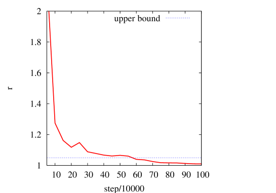
Figure 1: Estimate of potential scale reduction shown as a function of the number of Markov chain Monte Carlo steps. The upper bound we require for convergence is shown as a horizontal line.

Here, we define $r\equiv$max${}_{k}\{\sqrt{\hat{R}_{k}}\}$. Values of $r<1.05$ are considered to signify convergence and compatibility of the chains, since we could only hope to decrease the scale of any of the input parameter distributions by at most $5\%$ by performing further Markov Chain steps. In Fig. 1, we show the quantity $r$ as a function of step number. $r<1.05$ is met already for 600 000 steps indicating adequate convergence, although for the results we present below we we always use the full 9$\times$1 000 000 sample.

III Likelihood Maps

The number of input parameters exceeds the number of data and the likelihood shows a rough degeneracy along directions which give iso-lines of $\Omega_{DM}h^{2}$. The parameters of the best-fit point of the MCMC do not therefore supply us with much information, but the value of the likelihood at that point is interesting: a very small value would indicate a high $\chi^{2}$ and therefore a bad fit. The best-fit point sampled by the MCMC with 7d input parameter space was

$$m_{0}=964\mbox{~{}GeV},\ M_{1/2}=341\mbox{~{}GeV},\ A_{0}=1394\mbox{~{}GeV},$$

$$m_{b}(m_{b})=4.18\mbox{~{}GeV},\ m_{t}=173.0\mbox{~{}GeV},\$$

$$\alpha_{s}(M_{Z})=0.1185,\ \tan\beta=57.9,$$ (23)

leading to predictions of $\delta(g-2)_{\mu}/2=1.8\times 10^{-9}$, $BR(b\rightarrow s\gamma)=3.63\times 10^{-4}$ and $\Omega_{DM}h^{2}=0.1124$ and corresponding to a combined likelihood (ignoring normalisation constants, as stated above) of ${\mathcal{L}}=0.95$. The point is within the $A^{0}-$pole region, and the centrality of predicted observables gives us confidence that mSUGRA can fit well to current data. The efficiency of the MCMC algorithm is quite small: only 4.1$\%$. This reflects the fact that the thickness of WMAP-allowed volume is small, making it difficult to sample efficiently.

We display binned sampled likelihood distributions in Figs. 2a-2f for the full $m_{t}$, $m_{b}(m_{b})$, $\alpha_{s}(M_{Z})^{\overline{MS}}$, $m_{0}$, $A_{0}$, $\tan\beta$ and $M_{1/2}$ parameter space. The unseen dimensions in each figure have been marginalised with flat priors. All 2-d or 1-d marginalisations in this paper assume a flat prior (within the ranges of parameters considered in Table 1) in all unseen dimensions (or in other words, the likelihood is integrated over them with equal weight). One can view the marginalisation probabilistically, or just as a means of viewing the higher dimensional parameter space.

Figure 2: Likelihood maps of mSUGRA parameter space. The graphs show the likelihood distributions sampled from 7d parameter space and marginalised down to two. The likelihood (relative to the likelihood in the highest bin) is displayed by reference to the bar on the right hand side of each plot. The contours show the 68$\%$ and $95\%$ confidence level limits.

We have used 75$\times$75 bins, normalising the likelihood in each bin to the maximum likelihood in any bin in each 2d plane.

In each plot, the $h^{0}$ pole $s$-channel resonant annihilation region is present close to the lowest values of $M_{1/2}$. It can be seen as a vertical sliver in the top-left hand corner of the $m_{0}-M_{1/2}$ as in Fig. 2a and the slim band ranging across the bottom of Figs. 2d,2f. The bright region in Fig. 2a at low values of $m_{0}$ is primarily a co-annihilation region where slepton-neutralino annihilation contributes significantly to the depletion of the neutralino relic density in the early universe. However, at the lowest values of $m_{0}$ and $M_{1/2}$ values visible on the graph, the bulk region resides, being continuously connected to the co-annihilation tail, as shown in Ref. Ellis:2003cw . The pseudoscalar Higgs ($A^{0}$) $s$-channel annihilation channel occurs at high $\tan\beta=50-60$ and in the intermediate areas of $m_{0}=500-1600$ GeV, $M_{1/2}=250-1400$ GeV. In the literature, the most common way to display mSUGRA results is to present them in 2d in the $m_{0}$-$M_{1/2}$ plane, where thin strips are observed (see for example Ref. Ellis:2004tc ) that are consistent with the WMAP constraint upon $\Omega_{DM}h^{2}$. Fig. 2a demonstrates (in corroboration with Refs. Baltz:2004aw ; Stark:2005mp ) that the strips are truly a result of picking a 2d hyper-surface in parameter space: if one performs a full multi-dimensional scan, there is a large region in the $m_{0}$-$M_{1/2}$ plane that is consistent with the data. The bottom right hand side corner of Fig. 2a is ruled out primarily by the fact that the lightest supersymmetric particle (LSP) is charged. Large $M_{1/2}$ is disfavoured by the $(g-2)_{\mu}$ result. The bottom left-hand corner of Fig. 2a is ruled out by a combination of dark matter and direct search constraints. We see an interesting correlation between $m_{0}$ and $\tan\beta$ in Fig. 2b: the region extending to low $\tan\beta$ and low $m_{0}$ is essentially the stau co-annihilation/bulk region.

Figure 3: Likelihood distributions of masses in mSUGRA. The graphs show the likelihood distributions marginalised down to 2d. The likelihood (relative to the likelihood in the highest bin) is displayed by reference to the bar on the right hand side of each plot. The contours show the 68$\%$ and $95\%$ confidence level limits.

We display some binned likelihood distributions of MSSM particle masses in Figs. 3a-3c that are relevant for dark matter annihilation. In Fig. 3a, the $A^{0}$-pole resonance region is clearly discernable: at just above a line $2m_{\chi_{1}^{0}}=M_{A^{0}}$ and just below it, there is just enough annihilation to produce the observed relic density. Throughout much of the parameter space ($M_{A}<1$ TeV), the exact resonance condition depletes the relic density $\Omega_{DM}h^{2}$ to be too small. At around $M_{A}\sim 1$ TeV, exact resonance is required in order to sufficiently deplete the relic dark matter density. The rest of the likelihood density is spread over the dark part of the plot and is mostly too diffuse to be visible. In Fig. 3b, there are two detectable regions: the small one with the maximum 2d binned likelihood at the lowest possible values of $m_{\chi_{1}^{0}}$ corresponds to the $h^{0}$-pole region. The larger upper high likelihood region is an amalgam of the co-annihilation and $A^{0}$-pole regions. As a by-product we see that values of $m_{h}>126$ GeV are disfavoured in the mSUGRA model. In Fig. 3c, the stau co-annihilation region is visible as the diagonal dark line and the $h^{0}$-pole region as the lower likelihood horizontal dark line. The rest of the likelihood density is diffusely distributed in between these two extremes. We have shown the likelihood distribution for lightest chargino and slepton masses in Fig. 3d. Unfortunately, most of the likelihood is in a region where the well-known tri-lepton search channel Abazov:2005ku at the Tevatron is rather difficult. With 8 fb^-1 of integrated luminosity, this search channel requires $m_{\chi_{1}^{\pm}}<m_{\tilde{l}}$, $m_{\chi_{1}^{\pm}}<250$ for a discovery future .

Figure 4: (a) Selected sparticle mass likelihood distributions in mSUGRA, (b) stau-neutralino mass difference likelihood distribution where the insert shows a blow-up of the quasi mass-degenerate region. (c) branching ratio for the decay $B_{s}\rightarrow\mu^{+}\mu^{-}$. The Tevatron upper bound is displayed by a vertical line. (d) Likelihood density marginalised to the 2d plane $BR(B_{s}\rightarrow\mu^{+}\mu^{-})$ versus $M_{1/2}$. (e) Correlation between $BR(B_{s}\rightarrow\mu^{+}\mu^{-})$ and $(g-2)_{\mu}$. (f) Likelihood marginalised to the $\tan\beta$-$M_{A}$ plane. The contours show the 68$\%$ and $95\%$ confidence level limits.

We show the sampled likelihood distribution for $m_{{\tilde{l}}_{R}}$, $m_{\tilde{g}}$, $m_{{\tilde{t}}_{1}}$ and $m_{{\tilde{q}}_{L}}$ in Fig. 4a. The likelihood distributions have been placed into 75 bins of widths that are equal for the different types of sparticles. They are each normalised to an integrated likelihood of 1. The spike at low values of the gluino mass corresponds to the $h^{0}$-pole region of mSUGRA. This spike has a good chance of being covered at the Tevatron experiments before the LHC starts running future . It should be noted that upper limits upon the scalar sparticle masses inferred from Fig. 4a are due largely to the definition of the range of the initial parameters ($m_{0}$ being less than 2 TeV). Nevertheless, it is clear that there is already some preference from the combined data for various ranges of sparticle masses and upper bounds upon the gaugino masses. For example, values of $m_{\tilde{g}}>3.5$ TeV and $m_{\tilde{g}}=400-800$ GeV are disfavoured, as well as $m_{{\tilde{q}}_{L}}<800$ GeV. In Fig. 4b, the mass splitting between the lightest stau and lightest neutralino is shown. The insert in the figure displays the quasi-degenerate co-annihilation region at low mass splittings. The peaked region at $m_{{\tilde{\tau}}_{1}}-m_{\chi_{1}^{0}}<$10 GeV is likely to be difficult to discern at the Large Hadron Collider (LHC). One would wish to measure decays of the lightest staus in order to check the co-annihilation region, but reconstructing a relevant soft $\tau$ resulting from such a decay is likely to prove problematic. On the other hand, a linear collider with sufficient energy to produce sparticles could provide the necessary information Nojiri:1996fp ; Bambade:2004tq . The predicted likelihood distribution of the $B_{s}\rightarrow\mu^{+}\mu^{-}$ branching ratio is shown in Fig. 4c. Possible values for this observable were found with a random scan of unconstrained MSSM parameter space in Ref. Dedes:2004yc (no likelihood distribution was given). The region to the right hand side of the vertical line is ruled out from the combined CDF/D0 95$\%$C.L. exclusion Acosta:2004xj ; Abazov:2004dj limit $BR(B_{s}^{0}\rightarrow\mu^{+}\mu^{-})<3.4\times 10^{-7}$. We have not cut points violating this constraint, but this has negligible effect since there are only a small number of them. The 2d marginalisation of the branching ratio versus $M_{1/2}$ shows a peak at very low $M_{1/2}$ values, as Fig. 4d displays. This indicates that the spike in Fig. 4c at branching ratios of about $10^{-8.6}$ is due to the $h^{0}$-pole region. Lowering the empirical upper bound on the $B_{s}\rightarrow\mu^{+}\mu^{-}$ branching ratio will significantly cut into the allowed mSUGRA parameter space. A significant lowering of the bound upon this branching ratio is expected in the coming years from the Tevatron experiments and from LHCb. For example, it is estimated future that the Tevatron could exclude a branching ratio of more than $2\times 10^{-8}$ with 8 fb^-1 of integrated luminosity. This corresponds to ruling out 29$\%$ of the currently allowed likelihood density. Predictions for $BR(B_{s}\rightarrow\mu^{+}\mu^{-})$ were correlated with those for $(g-2)_{\mu}$ in Ref. Dedes:2001fv in mSUGRA. For a given mSUGRA parameter point, a correlation was shown when $\tan\beta$ was varied. The authors conclude that for high $\tan\beta$, an enhancement of $BR(B_{s}\rightarrow\mu^{+}\mu^{-})$ is implied by the $(g-2)_{\mu}$ measurements. We re-examine this statement in view of the full dimensionality of the mSUGRA parameter space in Fig. 4e. The correlation is seen to be far from perfect, the likelihood distribution being highly smeared in terms of the two measurements. Nevertheless, there is a mild correlation between $BR(B_{s}\rightarrow\mu^{+}\mu^{-})$ and the SUSY contribution to $(g-2)_{\mu}$ at the highest likelihoods, as evidenced by the bright oblique stripe in Fig. 4e. In Fig. 4f, we show the likelihood distribution in the $\tan\beta$-$m_{A}$ plane. There is a significant amount of likelihood density towards the top left-hand side of the plot, where the Tevatron is expected to have sensitivity future (covering $\tan\beta>40$ for $m_{A}<240$ GeV for 8fb^-1 of integrated luminosity). LHC experiments should be able to observe the $A^{0}$ for the entire high likelihood range Armstrong:1994it .

We now ask what are the likelihoods of the different regions of relic density depletion in mSUGRA parameter space. In order to sharply delineate the regions, we define them as follows: the co-annihilation region is defined such that $m_{\chi_{1}^{0}}$ is within $10\%$ of $m_{{\tilde{\tau}}_{1}}$. The $h^{0}/A^{0}$-pole regions have $2m_{\chi_{1}^{0}}$ within $10\%$ of $m_{h^{0}}$, $m_{A^{0}}$ respectively. Stop co-annihilation requires a broader definition: it is defined such that $m_{\chi_{1}^{0}}$ is within 30$\%$ of $m_{{\tilde{t}}_{1}}$, since the annihilation is so much more efficient Boehm:9911 ; arnie ; Ellis:2001nx than in the other regions. A better defined procedure might perhaps be to determine regions on the basis of the dominant annihilation mechanism, but since we are only looking for a rough indication of the region involved, the procedure adopted here will suffice. Points that fall in between any of the sharp definitions are either from the bulk region or in the smaller tails of the likelihood distribution.

Table 4: Likelihood of being in a certain region of mSUGRA parameter space.

Region	likelihood
$h^{0}$ pole	0.02$\pm$0.01
$A^{0}$ pole	0.41$\pm$0.03
$\tilde{\tau}$ co-annihilation	0.27$\pm$0.04
$\tilde{t}$ co-annihilation	$(2.1\pm 4.8)\times 10^{-4}$

The likelihoods of these regions are shown in Table 4. We estimate the uncertainty by calculating the standard deviation on the 9 independent Markov chain samples. The quoted error thus reflects an uncertainty due not to experimental errors, but to a to finite simulation time of the Markov chain. We see that the $h^{0}$-pole region has a relatively low likelihood whereas for the $A^{0}$-pole and $\tau$ co-annihilation regions the likelihood is larger. From the table, we see that the $\tilde{t}$-co-annihilation region, although uncertain due to the low statistics, is negligible, and we now investigate why this is the case.

The suppression of the stop-co-annihilation region comes from essentially two effects: firstly, as already apparent from Ref. Ellis:2001nx , finding a suitable stop co-annihilation region which is compatible with both the $(g-2)_{\mu}$ and $BR[b\rightarrow s\gamma]$ measurements is problematic. Secondly, the central value of $m_{t}$ has come down since ref. Ellis:2001nx . The dominant radiative corrections to $m_{h^{0}}$ are highly correlated with $m_{t}$ Allanach:2004rh , with the consequence that the lower predicted Higgs mass now rules out more of the stop co-annihilation region. We illustrate these points in Fig. 5 along the $m_{0}$ direction for given values of the other mSUGRA parameters (stated in the caption).

Figure 5: A line through the stop co-annihilation region in mSUGRA: $\tan\beta=10$, $M_{1/2}=350$ GeV, $A_{0}=-2000$ GeV and central Standard Model inputs. (a) dark matter relic density, fractional stop-neutralino mass splitting $\Delta\equiv(m_{{\tilde{t}}_{1}}-m_{\chi_{1}^{0}})/m_{\chi_{1}^{0}}$ and light Higgs mass. The horizontal lines show the 1$\sigma$ WMAP-derived limits upon $\Omega_{DM}h^{2}$ derived from Eq. 4, (b) muon magnetic moment and $BR[b\rightarrow s\gamma]$ predictions.

In Fig. 5a, we plot the fractional stop-neutralino mass splitting $\Delta$ alongside the neutralino relic density $\Omega_{DM}h^{2}$. We see that the fractional mass splitting takes values between 0.1 and 0.23 in the range of $m_{0}$ shown. This is the stop-co-annihilation regime, and we see that around $m_{0}\sim 786$ GeV, $\Delta\sim 0.2$ corresponding to $\Omega_{DM}h^{2}$ roughly compatible with the WMAP constraint. Unfortunately, we also see that the lightest CP-even Higgs mass is predicted to be 110.3 GeV here and is ruled out by the LEP2 Higgs limits shown in Table 3 ($\sin^{2}(\beta-\alpha)=1.0$) for this range of parameters). This problem is remedied by going to higher values of $m_{t}$, since $m_{h^{0}}$ then goes up, but of course this comes with an associated penalty in the likelihood from being away from the empirically central values of $m_{t}$. In Fig. 5b, we display predictions for $BR[b\rightarrow s\gamma]$ and $\delta(g-2)_{\mu}/2$ along the chosen range for $m_{0}$. These predictions are both lower than the empirically derived constraints in the region where the dark matter relic density is in accordance with the WMAP constraint: including errors in the theoretical prediction as described in the previous section, $BR[b\rightarrow s\gamma]$ is 1.95$\sigma$ lower than the central value and $\delta(g-2)_{\mu}/2$ is 1.6$\sigma$ lower. It turns out that these predictions are not very sensitive to changes in $m_{t}$ and so their likelihood penalty tends to apply for the higher values. However, lower values of $(-A_{0})$ require lower $m_{0}$ in order to fit the dark matter constraint and pick up a bigger likelihood constraint from the egregious prediction of $BR[b\rightarrow s\gamma]$. These findings are in rough agreement with those of Ref. Ellis:2001nx except for the more restrictive Higgs bounds, which are a consequence of the lower experimental value of $m_{t}$. Ref. Ellis:2001nx only applies 2$\sigma$ bounds on both $(g-2)_{\mu}$ and $BR[b\rightarrow s\gamma]$, whereas our results take into account the likelihood penalty paid by the fact that neither prediction is close to its central value near the stop co-annihilation region, which then becomes disfavoured compared to the other regions (where an almost perfect fit is possible). There is also a volume effect: in Table 4, the likelihoods we calculate are integrated over the relevant region. Thus regions that are very small, such as the stop co-annihilation region, will tend to have a smaller likelihood than other, larger regions. In analyses in following sections, stop co-annihilation also turns out to have negligible likelihood and so we will neglect it from the results.

As an aside, we note that the decay chain ${{\tilde{q}}_{L}}\rightarrow{\chi_{2}^{0}}\rightarrow{\tilde{l}}_{R}\rightarrow\chi_{1}^{0}$ exists with a likelihood of $0.24\pm 0.04$ (this number is just based upon the mass ordering and does not take into account the branching ratio for the chain). The existence of such a chain allows the extraction of several functions of sparticle masses from kinematic end-points and they have been used in many LHC analyses, for example Refs. Armstrong:1994it ; Allanach:2000kt ; Weiglein:2004hn .

IV Theoretical Uncertainty

Table 5: Likelihood of being in a certain region of mSUGRA parameter space including theoretical uncertainties in the sparticle spectrum calculation.

Region	likelihood
$h^{0}$ pole	0.03$\pm$0.01
$A^{0}$ pole	0.41$\pm$0.05
co-annihilation	0.26$\pm$0.08

Theoretical uncertainties in the sparticle mass predictions have been shown to produce non-negligible effects in fits to data Allanach:2003jw , including fits to the relic density Allanach:2004jh ; Allanach:2004xn ; Belanger:2005jk . In this section, we perform a second MCMC analysis taking theoretical uncertainty into account in order to estimate the size of its effect. SOFTSUSY performs the Higgs potential minimisation then calculates sparticle pole masses at a scale $M_{SUSY}=\sqrt{m_{{\tilde{t}}_{1}}m_{{\tilde{t}}_{2}}}$. This scale is chosen because it is hoped that loop corrections to the pole mass corrections that are not yet taken into account (typically two-loop corrections) are small at this scale. In order to estimate the size of theoretical uncertainties, we vary this scale by a factor of two in either direction (but it is always constrained to be greater than $M_{Z}$). Implementation of the uncertainty in the MCMC algorithm is simple: we simply add an input parameter $x$ which is bounded between 0.5 and 2, giving the factor by which $M_{SUSY}$ is to be multiplied. The MCMC is then re-run as before and explores the full 8d parameter space (including $x$) accordingly.

Such a procedure automatically takes into account the correlations in predictions due to correlated theoretical uncertainties in the sparticle mass predictions. The likelihoods of the three mSUGRA regions are shown in Table 5. The likelihoods are approximately equal to those for the 7d case, as a comparison to Table 4 indicates. In fact, comparing results and plots produced with and without theoretical uncertainties, the results are generally very similar. This indicates that the theoretical uncertainties don’t make a huge difference to the 1d and 2d marginalisations compared to those coming from the data. The decay chain ${{\tilde{q}}_{L}}\rightarrow{\chi_{2}^{0}}\rightarrow{\tilde{l}}_{R}\rightarrow{\chi_{1}^{0}}$ has a likelihood of $0.22\pm 0.08$, not significantly different to the case when theoretical uncertainties were not taken into account.

We show two of the 2d marginalised likelihoods in Figs. 6a,6b. Comparing with Fig. 2, we see that Fig. 6 shows no significant effects deriving from theoretical errors. Marginalising mass likelihood distributions down to 1d (as in Fig. 4a for example), one obtains distributions that are identical to the 7d case except for small statistical fluctuations.

Figure 6: Likelihood maps of mSUGRA parameter space including theoretical uncertainty. The graphs show the likelihood distributions sampled from 8d parameter space and marginalised down to two. The likelihood (relative to the likelihood in the highest bin) is displayed by reference to the bar on the right hand side of each plot. The contours show the 68$\%$ and $95\%$ confidence level limits.

V Other Sources of Dark Matter

For completeness, we may ask how robust our results are with respect to the assumption that non thermal-neutralino contributions to $\Omega_{DM}$ are negligible. Thus, we allow the predicted amount of thermal neutralino relic density $p_{\Omega_{DM}h^{2}}$ (assuming some mSUGRA point $s$) to be some fraction of the total relic predicted relic density $\Omega_{DM}^{tot}h^{2}$:

$$\lambda=\frac{p_{\Omega_{DM}h^{2}}}{\Omega_{DM}^{tot}h^{2}},\qquad 0\leq\lambda\leq 1.$$ (24)

Thus, the total amount of dark matter predicted is $p_{\Omega_{DM}h^{2}}/\lambda$ and, assuming a flat pdf for $\lambda$ as shown in Fig. 7a, we obtain the likelihood penalty for a given SUSY dark matter prediction

$${\mathcal{L}}_{\Omega_{DM}h^{2}}=\int^{1}_{0}d\lambda\ \frac{1}{\sqrt{2\pi}s_{\Omega_{DM}h^{2}}(\lambda)}\exp\left[\frac{-(m_{\Omega_{DM}h^{2}}-p_{\Omega_{DM}h^{2}}/\lambda)^{2}}{2s_{\Omega_{DM}h^{2}}(\lambda)^{2}}\right],$$ (25)

where

$$s_{\Omega_{DM}h^{2}}(\lambda) \equiv 0.0081\ \theta(p_{\Omega_{DM}h^{2}}/\lambda-m_{\Omega_{DM}h^{2}})+$$ (26)

$$0.0091\ \theta(-p_{\Omega_{DM}h^{2}}/\lambda+m_{\Omega_{DM}h^{2}})$$

in accordance with the asymmetric errors in Eq. 4. $\theta(x)$ is the Heavisde step function, $\theta(x)=1$ for all $x\geq 0$, $\theta(x)=0$ for all $x<0$. We calculate Eq. 25 numerically and display it in Fig. 7b, where it is contrasted with the old dark matter likelihood penalty that assumes that all dark matter is of thermal neutralino origin.

Figure 7: (a) $p(\lambda|m_{\Omega_{DM}h^{2}})$, the probability distribution assumed for $\lambda$, the ratio of predicted SUSY dark matter to total dark matter, given some measured value $m_{\Omega_{DM}h^{2}}$. (b) Comparison of the likelihood penalty ${\mathcal{L}}_{\Omega_{DM}h^{2}}$ paid for a prediction of SUSY dark matter $p_{\Omega_{DM}h^{2}}$ with (“extra DM allowed”) and without (“no extra DM allowed”) the allowance of non thermal-neutralino dark matter.

The figure shows that if the relic density is too high, a severe likelihood penalty applies (similar to the “no extra DM allowed” case) but a much less severe penalty applies if the prediction is below the central value of the observed WMAP value in Eq. 4. The additional contribution to $\Omega h^{2}$ is assumed to be provided by some non thermal-neutralino source (late decays or hidden sector dark matter for example) leszek . The rest of the analysis proceeds exactly as in section III (i.e. without simultaneously taking theoretical uncertainty into account).

Table 6: Likelihood of being in a certain region of mSUGRA parameter space including possible an additional contribution from non thermal-neutralino dark matter.

Region	likelihood
$h^{0}$ pole	0.04$\pm$0.01
$A^{0}$ pole	0.52$\pm$0.02
co-annihilation	0.14$\pm$0.02

The MCMC algorithm turns out to be much more efficient once we drop the assumption that the cold dark matter consist only of neutralinos: 19.9$\%$ efficiency was achieved compared to 4.1$\%$. One consequence of this is that statistical fluctuations in the results are smaller. The likelihoods in each region are shown in Table 6. A comparison of Tables 4,6 shows that annihilation through $A^{0}$ pole has acquired a significantly larger likelihood through allowing for other forms of dark matter. The higgs-pole and co-annihilation regions are still, within statistics, compatible with their previous likelihoods. All of the listed uncertainties have decreased, due to the additional efficiency.

Figure 8: Likelihood maps of mSUGRA parameter space allowing for non thermal-neutralino contributions to the dark matter relic density. The graphs show the likelihood distributions sampled from 7d parameter space and marginalised down to two. The likelihood (relative to the likelihood in the highest bin) is displayed by reference to the bar on the right hand side of each plot. The contours show the 68$\%$ and $95\%$ confidence level limits.

Fig. 8a shows the likelihood map marginalised to the $M_{1/2}-m_{0}$ plane. Comparing it to Fig. 2a, we see a very similar picture except for the fact that the higher volume of likelihood in the $A^{0}$-pole region is evident. The same comment can be made of all of the plots analogous to the ones in to Fig. 2: we show the likelihood marginalised to the $m_{0}-A_{0}$ plane in Fig. 8 as an example. There are no other qualitative changes in any of the plots, and indeed the likelihood distributions marginalised to the $A_{0}-\tan\beta$ and $M_{1/2}-A_{0}$ planes (analogous to Figs. 2e,f) are identical by eye, except for being smoother due to the increased efficiency. Likelihoods of sparticle masses also look the same, except for the spike in the gluino mass, which has twice as much likelihood. As mentioned before, this spike is due mainly to the light $h^{0}$-pole region which is subject to relatively large fluctuations, as Tables 4,6 illustrate. We cannot conclude that the $h^{0}$-pole region obtains more integrated likelihood by admitting non thermal-neutralino components to the relic density because the statistics in the MCMC algorithm are not high enough.

One distribution that does significantly change shape is that of $BR(B_{s}\rightarrow\mu^{+}\mu^{-})$. We show its marginalised distribution after dropping the lower likelihood penalties on $\Omega_{DM}h^{2}$ from the MCMC algorithm procedure in Fig. 9 as the histogram marked “extra DM allowed”. For the purpose of comparison, the default calculation where we assume all dark matter to be thermal neutralinos from Fig. 4c is also displayed, being marked “no extra DM allowed”. Comparing the two distributions, we see a broader distribution due to the enhanced $A^{0}$-pole annihilation region when additional components are allowed in the fit. The $A^{0}$-pole region has higher $\tan\beta$, and therefore higher values for the branching ratio.

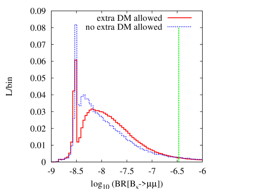
Figure 9: Investigation on the effects of allowing for a non thermal-neutralino component of dark matter in the branching ratios for the decay $B_{s}\rightarrow\mu^{+}\mu^{-}$ in mSUGRA. The current Tevatron upper limit is displayed by a vertical line.

The estimated amount of likelihood that could be covered by Tevatron measurements with 8 fb^-1 of integrated luminosity increases by 6$\%$ to 35$\%$ of the currently allowed density due to the presence of non thermal-neutralino dark matter contributions.

VI Conclusions

Previous studies of mSUGRA in the context of dark matter and particle physics constraints have tended to not use the full dimensionality of the parameter space, and to have put hard 95$\%$ (C.L.) limits on predictions. Here, in the full dimensionality of parameter space, we include all of the information in a likelihood fit, so that violating one constraint slightly might be traded against fitting another one better in a consistent manner. Although there is plenty of qualitative information about possible dark matter annihilation regions in mSUGRA in the literature, this paper gives a quantitative calculation of the likelihood distributions in the full dimensionality of the parameter space. However, the most important contribution of this paper lies in the implications of the results to particle physics.

We have successfully employed an MCMC algorithm to provide likelihood maps of the full 7d input parameter space of mSUGRA. By using a statistical test, we have shown that the likelihood distributions have achieved good convergence before a total of 9$\times 10^{6}$ samplings of the likelihood. We have presented the likelihood marginalised down to each 2d mSUGRA parameter pair. Such plots provide the totality of the current information we have about the model given the experimental constraints and are quantitative results. Theoretical uncertainties in the sparticle spectrum calculation broaden a couple of the distributions a little but do not change them radically.

The main new contribution of this paper is to our knowledge of what current constraints on mSUGRA mean for particle physics in a quantitative sense. Marginalised 1d likelihood distributions of quantities such as sparticle masses (or mass differences) already show some significant structure from the data, providing interesting information for future collider searches. In particular, the likelihood of the “golden cascade” ${\tilde{q}}_{L}\rightarrow\chi_{2}^{0}\rightarrow{\tilde{l}}_{R}\rightarrow\chi_{1}^{0}$ being kinematically allowed is 24$\pm 4\%$. $m_{{\tilde{\tau}}_{1}}-m_{\chi_{1}^{0}}$ is peaked below 10 GeV, implying that stau reconstruction at hadron colliders could be problematic at the LHC. Integrating the likelihood density, we find the likelihood of $m_{{\tilde{\tau}}_{1}}-m_{\chi_{1}^{0}}<10$ GeV is 19.9$\%$. Our likelihood distributions for $BR(B_{s}\rightarrow\mu^{+}\mu^{-})$ corroborate the conclusions of ref. Ellis:2005sc : that current bounds upon the branching ratio do not yet place significant constraints upon mSUGRA once other constraints have been taken into account, but any improvement on the upper bounds constrain the currently available parameter space. The quantitative results on $BR(B_{s}\rightarrow\mu^{+}\mu^{-})$ are particularly important: if the Tevatron experiments can reach down to 2$\times 10^{-8}$, they will cover 29$\%$ of the mSUGRA likelihood, or 35$\%$ if we allow the possibility of additional contributions to the relic density other than thermal neutralinos.

We have shown that the correlation between $BR(B_{s}\rightarrow\mu^{+}\mu^{-})$ and $\delta(g-2)_{\mu}$ noticed in Ref. Dedes:2001fv is much diluted once simultaneous variations of all mSUGRA parameters are taken into account. The $A^{0}$-pole annihilation region and the stau co-annihilation region each have approximately an order of magnitude more likelihood than the $h^{0}$-pole region. Stop co-annihilation is highly disfavoured compared to these other regions due to more restrictive Higgs mass constraints coming from a lower value of $m_{t}$, as well as the $BR(B_{s}\rightarrow\mu^{+}\mu^{-})$ and $\delta(g-2)_{\mu}$ predictions. The light $h^{0}-$pole region just survives the LEP2 Higgs mass constraints despite the new reduced top mass value albeit with a reduced likelihood (in the usual frequentist language, it’s outside the 95$\%$ confidence level but not the 99$\%$ one). The light $h^{0}$-pole region has more likelihood if one allows additional non thermal-neutralino components of dark matter.

The analysis of Ref. Ellis:2004tc includes $M_{W}$ and $\sin^{2}\theta_{eff}^{l}$ in the $\chi^{2}$ statistic, excluding $M_{1/2}>1500(600)$ GeV at the 90$\%$ confidence level for $m_{t}=178$ GeV and $\tan\beta=50(10)$ respectively. These numbers are not exactly reproduced in the present analysis for several reasons: we use a more up-to-date value of $m_{t}$, we vary $m_{t}$, $m_{b}$, $\alpha_{s}(M_{Z})$ and $\tan\beta$ simultaneously with the other mSUGRA parameters and we do not include $M_{W}$, $\sin^{2}\theta_{eff}^{l}$ in the fit. Indeed, one may wonder about introducing a posteriori bias as a result of only picking these two precision electroweak observables, since they are the two that show a preference for a SUSY contribution. Other observables would presumably prefer heavier SUSY particles. However, $M_{W}$ and $\sin^{2}\theta_{eff}^{l}$ do show a preference for lower $M_{1/2}$ for $m_{t}=178$ GeV. Having said that, our results are not wildly different, as an examination of Fig. 2a shows.

We suspect that the MCMC techniques exemplified here could be found extremely useful in SUSY fitting programs such as FITTINO Bechtle:2004pc and SFITTER Lafaye:2004cn in order to provide a likelihood profile of the parameter space, including secondary local minima. These programs are designed to fit more general MSSM models than mSUGRA to data, with an associated increase in the number of free input parameters, so the linear calculating time of MCMCs ought to be very useful.

While our results presented for mSUGRA are in themselves interesting, it is obvious that the method will be applicable in a much wider range of circumstances. Once new observables become relevant, such as some LHC end-points, for example, it would be trivial to include them into the likelihood and re-perform the MCMC whitey . The method should be equally applicable to other models, and provided enough CPU power is to hand, could provide likelihood maps for models with even more parameters and/or detailed electroweak fits.

Appendix A Toy Models and Sampling

By definition, a sampler able to sample correctly from a pdf $p({\mathbf{x}})$ must generate a list of ${\mathbf{x}}$ values whose local density, at large step-numbers, is proportional to the probability density $p({\mathbf{x}})$ at each part of the space (in the preceding parts of the paper we have set this pdf to be the likelihood). The value of the constant of proportionality between the probability density and the local density of ${\mathbf{x}}$ values is unimportant, but the key point is that it is constant across the whole space.

It can sometimes be hard to implement a good sampler for a given probability distribution. In fact it is often easier to invent an algorithm which generates a sequence of ${\mathbf{x}}$ values, and which may superficially resemble a sampler, but which lacks constancy of proportionality over the space. We might call such algorithms pseudo-samplers as their output can sometimes resemble that of a true sampler, provided that the variation in proportionality is not too great across the space considered. Pseudo-samplers are sometimes useful (e.g. as a means of exploring a multidimensional space in which case sample density may be neither interesting nor the end product of the analysis).

In the present and in many other papers, however, sample density represents confidence in some particular part of parameter space, and is the final product of the analysis. Extreme care, then, must be taken to ensure that any creative modifications to established Markov Chain sampling techniques do not break the principle of detailed balance – the test which ensures that the algorithm remains a true sampler rather than a pseudo-sampler.

It is often desirable for Metropolis-Hastings type samplers to have an efficiency of about 25% for the acceptance of newly proposed points. Efficiencies much smaller than this may suggest that the proposal distribution is too wide and is too often proposing jumps to undesirable locations far away from the present point, leading to large statistical fluctuations in the result. Efficiencies much larger than this can be indicative of proposal distributions which are too narrow and may take too many steps to be practical to random-walk from one side of a region of high probability to the other. It is tempting, therefore, to adapt the present step size (i.e. proposal distribution width) on the basis of recent efficiency. With a couple of toy examples, however, we will illustrate that this is a dangerous path to follow, and we will demonstrate that it break the principle of detailed balance, and thus turns the Markov Chain algorithm from a sampler into a pseudo-sampler.

We take as our example the method used by Baltz and Gondolo Baltz:2004aw which is designed to keep the target efficiency of the authors’ Markov Chain close to 25%:

1. Double the current step size if the last three proposed points were all accepted

2. Halve the current step size of the last seven proposed points were all rejected.

We will refer the the above method as “the adaptive algorithm” and show that it fails to sample correctly from some simple distributions, a signature of detailed balance being broken.

Figure 10: Binned samples of the double Gaussian distribution $p_{dGau}(x)$. The normalisation is arbitrary and has no relevance here. (a) uses a Metropolis-Hastings algorithm and yields a good approximation whereas (b) uses the adaptive algorithm.

Take, for example, the 1-dimensional double Gaussian probability distribution $p_{dGau}(x)$ defined by

$$p_{dGau}(x)\propto g(x,0,1)+g(x,10,1/2),$$ (27)

where $g(x,m,\sigma)=\exp(-(x-m)^{2}/(2\sigma^{2}))$ is a Gaussian distribution of unit height and width $\sigma$ centred on $x=m$. Note that the Gaussian near the origin is wider than the Gaussian near $x=10$. This pdf mocks up the approximate situation along the $M_{1/2}$ direction in mSUGRA for large $m_{0}$, as Fig. 2a shows. The narrow Gaussian would then correspond to the light $h^{0}$-pole region, which is quite disconnected from the wider $A^{0}$-pole region. A Metropolis-Hastings algorithm (see section II) with a fixed Gaussian proposal pdf $Q(x)$ of width 5 was run for 2 000 000 steps and the binned result is shown in Figure 10a. It reproduces the target distribution very well. In contrast, Figure 10b shows what happens when the adaptive algorithm is run on $p_{dGau}(x)$. Clearly the result is very different to that in Figure 10a and is thus very wrong. The narrow Gaussian has been sampled many times more frequently than it should have been relative to the wider one near the origin.

The adaptive algorithm ensures that whenever the current point is in one of the two Gaussian regions, the step size is adjusted to be proportional to the width of that region. This adaptation is not immediate (seven successive rejections must occur before the step size is halved) but suppose for the moment that adaptation were to take place almost immediately. For the moment, let us also neglect random fluctuations of the step size. In such a limit, when the current point is in the left-hand Gaussian region, the step size is double what it is when the current point is in the right-hand region. Making a proposal for a jump from the region on the left to the region on the right, therefore, is something like a $10$-sigma event. In contrast, making the reverse proposal (from right to left) is more like a $20$-sigma event. In this limit, it is thus $e^{((20)^{2}-(10)^{2})/2}=e^{150}$ times more likely that jumps to the right get proposed than jumps to the left. This is a vast overestimate of the bias toward the narrow region for two reasons. Firstly, step size adaptation is not immediate (even when the step size is half of what it should be, quite a few steps occur before seven successive rejections). Secondly and more importantly, even when settled in one of the two regions, the adaptive step size makes excursions about its mean value. Excursions to very high step sizes (double or quadruple the average step size) are infrequent but still occur. When they do, they elevate the chance of proposing a jump from one region to another, and help to equilibrate between the two regions. Both of these effects reduce the bias favouring the narrow region, but still break detailed balance, and overall the right hand Gaussian is still sampled about 10 times more frequently than it should be.

Figure 11: Binned sampling of a Cauchy distribution $1/(1+x^{2})$ (shown in solid red line) truncated at $x=\pm 500$. (a) shows the result of direct sampling and yields a good approximation whereas (b) uses the adaptive algorithm.

For quite a different example, consider the truncated Cauchy distribution defined by

$$p_{cauchy}(x)\propto\begin{cases}1/(1+x^{2})&\mbox{if~{}}x>-500\mbox{~{}and~{}}x<500,\\ 0&\mbox{otherwise}.\end{cases}$$ (28)

A faithful sampling from this distribution is shown in Figure 11(a), and a mis-sampling using the adaptive algorithm is shown for comparison in Figure 11(b). Although there is better correspondence between the samples generated by the two methods than was the case earlier, it is nevertheless evident that there are large differences between the degrees to which the two methods have sampled the tails of the distribution. As a consequence, samples from the adaptive method have a root-mean-squared value of 7.6 compared to the value of 17.9 obtained by the true sampling. The cause of the discrepancy is again due to the very different scales in the cauchy distribution. Its core is very narrow with a width of order 1, but there are significant parts of probability also lodged in the tails many orders of magnitude away. The adaptive method has to raise and lower the step size frequently to sample from the whole dynamic range, and in doing so it has to break detailed balance many times, resulting in the cumulative effect of an overall order of magnitude bias in the tails.

References

- (1) S. P. Martin, hep-ph/9709356.
- (2) J. R. Ellis, K. A. Olive, Y. Santoso, and V. C. Spanos, Phys. Lett. B588 (2004) 7–16, hep-ph/0312262.
- (3) L. Roszkowski, R. Ruiz de Austri and K.-Y. Choi, JHEP 0508 (2005) 080 [arXiv:hep-ph/0408227]; D.G. Cerdeno et al, hep-ph/0509275.
- (4) L. Covi, J. E. Kim, L. Roszkowski Phys. Rev. Lett. 82 (1999) 4180-4183, hep-ph/9905212; L. Covi, H. B. Kim, J. E. Kim, L. Roszkowski JHEP 0105 (2001) 033, hep-ph/0101009; L. Covi, L. Roszkowski, R. Ruiz de Austri and M. Small, JHEP 0406 (2004) 003 hep-ph/0402240.
- (5) J. R. Ellis, J. S. Hagelin, D. V. Nanopoulos, K. A. Olive, and M. Srednicki, Nucl. Phys. B238 (1984) 453–476.
- (6) H. Baer et. al., JHEP 07 (2002) 050, hep-ph/0205325.
- (7) J. R. Ellis, K. A. Olive, Y. Santoso, and V. C. Spanos, Phys. Lett. B565 (2003) 176–182, hep-ph/0303043.
- (8) M. Battaglia et. al., Eur. Phys. J. C33 (2004) 273–296, hep-ph/0306219.
- (9) J. R. Ellis, K. A. Olive, Y. Santoso, and V. C. Spanos, Phys. Rev. D69 (2004) 095004, hep-ph/0310356.
- (10) M. E. Gomez, T. Ibrahim, P. Nath and S. Skadhauge, Phys. Rev. D 70, 035014 (2004) [arXiv:hep-ph/0404025].
- (11) J. R. Ellis, S. Heinemeyer, K. A. Olive, and G. Weiglein, JHEP 02 (2005) 013, hep-ph/0411216.
- (12) ATLAS Collaboration, W. W. Armstrong et. al., CERN-LHCC-94-43.
- (13) D. N. Spergel et. al., Astrophys. J. Suppl. 148 (2003) 175, astro-ph/0302209.
- (14) C. L. Bennett et. al., Astrophys. J. Suppl. 148 (2003) 1, astro-ph/0302207.
- (15) B. C. Allanach, G. Belanger, F. Boudjema, and A. Pukhov, JHEP 12 (2004) 020, hep-ph/0410091.
- (16) K. Griest and D. Seckel, Phys. Rev. D43 (1991) 3191–3203.
- (17) M. Drees and M. M. Nojiri, Phys. Rev. D47 (1993) 376–408, hep-ph/9207234.
- (18) R. Arnowitt and P. Nath, Phys. Lett. B299 (1993) 58–63, hep-ph/9302317.
- (19) A. Djouadi, M. Drees, and J.-L. Kneur, hep-ph/0504090.
- (20) J. L. Feng, K. T. Matchev, and T. Moroi, Phys. Rev. Lett. 84 (2000) 2322–2325, hep-ph/9908309.
- (21) J. L. Feng, K. T. Matchev, and T. Moroi, Phys. Rev. D61 (2000) 075005, hep-ph/9909334.
- (22) J. L. Feng, K. T. Matchev, and F. Wilczek, Phys. Lett. B482 (2000) 388–399, hep-ph/0004043.
- (23) C. Boehm, A. Djouadi and M. Drees, Phys. Rev. D62 (2000) 035012 hep-ph/9911496.
- (24) R. Arnowitt, B. Dutta and Y. Santoso, Nucl. Phys. B606 (2001) 59 hep-ph/0102181.
- (25) J. R. Ellis, K. A. Olive and Y. Santoso, Astropart. Phys. 18 (2003) 395, hep-ph/0112113.
- (26) M. Brhlik, D. J. H. Chung, and G. L. Kane, Int. J. Mod. Phys. D10 (2001) 367, hep-ph/0005158.
- (27) M. Drees et. al., Phys. Rev. D63 (2001) 035008, hep-ph/0007202.
- (28) G. Polesello and D. R. Tovey, JHEP 05 (2004) 071, hep-ph/0403047.
- (29) P. Bambade, M. Berggren, F. Richard, and Z. Zhang, hep-ph/0406010.
- (30) B. C. Allanach, G. Belanger, F. Boudjema, A. Pukhov, and W. Porod, hep-ph/0402161.
- (31) T. Moroi, Y. Shimizu, and A. Yotsuyanagi, hep-ph/0505252.
- (32) J. L. Bourjaily and G. L. Kane, hep-ph/0501262.
- (33) L. Roszkowski, R. Ruiz de Austri, and T. Nihei, JHEP 08 (2001) 024, hep-ph/0106334.
- (34) H. Baer, C. Balazs, and A. Belyaev, JHEP 03 (2002) 042, hep-ph/0202076.
- (35) H. Baer and C. Balazs, JCAP 0305 (2003) 006, hep-ph/0303114.
- (36) U. Chattopadhyay, A. Corsetti, and P. Nath, Phys. Rev. D68 (2003) 035005, hep-ph/0303201.
- (37) A. B. Lahanas and D. V. Nanopoulos, Phys. Lett. B568 (2003) 55–62, hep-ph/0303130.
- (38) G. Belanger, F. Boudjema, A. Cottrant, A. Pukhov, and A. Semenov, hep-ph/0412309.
- (39) L. Roszkowski, Pramana 62 (2004) 389 hep-ph/0404052.
- (40) CDF and D0 Collaboration, M. Herndon, To appear in the proceedings of 32nd International Conference on High-Energy Physics (ICHEP 04), Beijing, China, 16-22 Aug 2004.
- (41) J. R. Ellis, K. A. Olive, and V. C. Spanos, hep-ph/0504196.
- (42) S. Profumo and C. E. Yaguna, Phys. Rev. D70 (2004) 095004, hep-ph/0407036.
- (43) L. S. Stark, P. Hafliger, A. Biland, and F. Pauss, hep-ph/0502197.
- (44) E. A. Baltz and P. Gondolo, JHEP 10 (2004) 052, hep-ph/0407039.
- (45) D. MacKay, Information Theory, Inference, and Learning Algorithms. Cambridge University Press, 2003.
- (46) B. C. Allanach, D. Grellscheid, and F. Quevedo, JHEP 07 (2004) 069, hep-ph/0406277.
- (47) O. Brein, hep-ph/0407340.
- (48) B. C. Allanach, J. P. J. Hetherington, M. A. Parker, and B. R. Webber, JHEP 08 (2000) 017, hep-ph/0005186.
- (49) B. C. Allanach, Comput. Phys. Commun. 143 (2002) 305–331, hep-ph/0104145.
- (50) S. Eidelman et. al., Phys. Lett. B 592 (2004) 1–end.
- (51) B. C. Allanach, A. Djouadi, J. L. Kneur, W. Porod, and P. Slavich, JHEP 09 (2004) 044, hep-ph/0406166.
- (52) ALEPH Collaboration, R. Barate et. al., Phys. Lett. B565 (2003) 61–75, hep-ex/0306033.
- (53) G. Degrassi, S. Heinemeyer, W. Hollik, P. Slavich, and G. Weiglein, Eur. Phys. J. C28 (2003) 133–143, hep-ph/0212020.
- (54) P. Skands et. al., JHEP 07 (2004) 036, hep-ph/0311123.
- (55) G. Belanger, F. Boudjema, A. Pukhov, and A. Semenov, Comput. Phys. Commun. 149 (2002) 103–120, hep-ph/0112278.
- (56) G. Belanger, F. Boudjema, A. Pukhov, and A. Semenov, hep-ph/0405253.
- (57) Muon g-2 Collaboration, G. W. Bennett et. al., Phys. Rev. Lett. 92 (2004) 161802, hep-ex/0401008.
- (58) M. Passera, J. Phys. G31 (2005) R75–R94, hep-ph/0411168.
- (59) J. F. de Troconiz and F. J. Yndurain, Phys. Rev. D71 (2005) 073008, hep-ph/0402285.
- (60) B. C. Allanach, A. Brignole, and L. E. Ibanez, JHEP 05 (2005) 030, hep-ph/0502151.
- (61) P. Gambino, U. Haisch, and M. Misiak, Phys. Rev. Lett. 94 (2005) 061803, hep-ph/0410155.
- (62) Heavy Flavour Averaging Group Collaboration. http://www.slac.stanford.edu/xorg/hfag.
- (63) CDF and D0 Collaboration, the Tevatron Electroweak Working Group, hep-ex/0507091.
- (64) A. Gelman and D. Rubin, Stat. Sci. 7 (1992) 457–472.
- (65) D0 Collaboration, V. M. Abazov et. al., hep-ex/0504032.
- (66) CDF and D0 Collaboration. See URL http://www-cdf.fnal.gov/physics/projections/.
- (67) M. M. Nojiri, K. Fujii, and T. Tsukamoto, Phys. Rev. D54 (1996) 6756–6776, hep-ph/9606370.
- (68) A. Dedes and B. T. Huffman, Phys. Lett. B600 (2004) 261–269, hep-ph/0407285.
- (69) CDF Collaboration, D. Acosta et. al., Phys. Rev. Lett. 93 (2004) 032001, hep-ex/0403032.
- (70) D0 Collaboration, V. M. Abazov et. al., Phys. Rev. Lett. 94 (2005) 071802, hep-ex/0410039.
- (71) CDF and D0 Collaboration, S. Dugad, To appear in the proceedings of the Hadron Collider Physics Symposium, Les Diablerets, Switzerland, 3-9 Jul 2005.
- (72) A. Dedes, H. K. Dreiner, and U. Nierste, Phys. Rev. Lett. 87 (2001) 251804, hep-ph/0108037.
- (73) B. C. Allanach, C. G. Lester, M. A. Parker, and B. R. Webber, JHEP 09 (2000) 004, hep-ph/0007009.
- (74) LHC/LC Study Group Collaboration, G. Weiglein et. al., hep-ph/0410364.
- (75) B. C. Allanach, S. Kraml, and W. Porod, JHEP 03 (2003) 016, hep-ph/0302102.
- (76) G. Belanger, S. Kraml, and A. Pukhov, hep-ph/0502079.
- (77) P. Bechtle, K. Desch, and P. Wienemann, hep-ph/0412012.
- (78) R. Lafaye, T. Plehn, and D. Zerwas, hep-ph/0404282.
- (79) M. White, C. Lester, and A. Parker, hep-ph/0508143.