For high precision measurements of $K$ decays, the presence of radiated photons cannot be neglected. The Monte Carlo simulations must include the radiative corrections in order to compute the correct event counting and efficiency calculations. In this paper we briefly describe a method for simulating such decays.

1 Introduction

Many measurements on $K$ decays have reached a statistical error close to 1% or less. With such precision, the presence of radiated photons, and in general the effect of radiative corrections, cannot be neglected. Furthermore, the treatment of the radiative corrections is explicitly required for the extraction of many physical quantities, such as the CKM matrix element $V_{us}$ and the phase shifts $\delta_{0}-\delta_{2}$, at precisions of a few percent (or above). Hence, it is mandatory to include the effect of radiated photons in the Monte Carlo (MC) simulations.

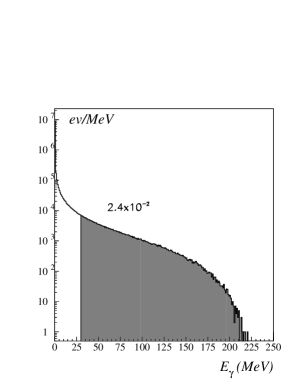
Figure 1: Energy spectrum for $K^{{0}}\rightarrow\pi e\nu\gamma$ MC decays. 2.4% of the events have $E_{\gamma}>30~{}\mbox{MeV}$.

There are two aspects of a measurement that are affected by the presence of radiated photons [1]: the geometrical acceptance and the counting of the events. About 2.4% of $K^{{0}}\rightarrow\pi e\nu\gamma$ decays have a photon with an energy above $30~{}\mbox{MeV}$, as shown in Fig. 1, corresponding to about 10% of the center-of-mass energy. These photons soften the momentum spectra of the electron and pion that are actually detected in an experiment, changing the geometrical acceptance and the distributions of kinematic quantities often used to select or count the number of signal events. If these effects are neglected, errors up to few percent can result in the measurement of a given branching ratio [2] [3].

2 Bremsstrahlung and infrared divergences

The main problem in simulating radiative decays is the presence of infrared divergences: the total decay width for single photon emission, computed at any fixed order in $\alpha$, is infinite. A finite value is obtained only by summing the decay widths for the real and virtual processes calculated to the same order in $\alpha$. As shown in Ref. [5], in the limit of soft photon energy, we can “re-sum” the probabilities for multiple photon emission to all order in $\alpha$. The rate for the decay process $i\to f$ accompanied by any number of soft photons with total energy less than $E_{\gamma}$ is given by:

$$\Gamma_{incl}(E_{\gamma})=\Gamma_{0}\left(\frac{E_{\gamma}}{\Lambda}\right)^{b}(1+O(b^{2})+O(E_{\gamma})).$$ (1)

Here $\Gamma_{0}$ is the unphysical decay width for the process $i\to f$ without final state photons, and $b$ is a function of the particle momenta, is positive and of order $\alpha$; it is given by:

$$b=-\frac{1}{8\pi^{2}}\sum_{m,n}\eta_{m}\eta_{n}e_{m}e_{n}\beta_{mn}^{-1}\ln\frac{1+\beta_{mn}}{1-\beta_{mn}},$$ (2)

where $m$ and $n$ run over all the external particles, $e_{n}$ is the charge of the particle $n$, $\eta=+1$ or $-1$ for an outgoing or incoming particle, and $\beta_{mn}$ is the relative velocity of the particles $n$ and $m$ in the rest frame of either:

$$\beta_{mn}=\left[1-\frac{m_{n}^{2}m_{m}^{2}}{(p_{n}\cdot p_{m})^{2}}\right]^{1/2}.$$ (3)

$\Lambda$ is an energy cut-off that can be chosen as the mass $M$ of the decaying particle.

Differentiating $\Gamma_{incl}(E_{\gamma})$ with respect to $E_{\gamma}$, we obtain an integrable differential distribution:

$$\frac{d\Gamma_{incl}}{dE_{\gamma}}=\Gamma_{0}b\frac{E_{\gamma}^{b-1}}{M^{b}}=\frac{d\Gamma_{Brem}}{dE_{\gamma}}\left(\frac{E_{\gamma}}{M}\right)^{b},$$ (4)

where we have neglected second order terms in $b$. To $O(\alpha$) this can be identified with the single-photon emission probability, and indeed, it can be written in terms of:

$$\frac{d\Gamma_{Brem}}{dE_{\gamma}}=\Gamma_{0}\frac{b}{E_{\gamma}}.$$ (5)

The presence of the extra factor $(E_{\gamma}/M)^{b}$ ensures the integrability of Eq. (4) in the limit $E_{\gamma}\to 0$.

In the derivation of Eq. (1), in Ref. [5], no explicit integration is required on the momenta of particles other than those of the photons. The result in Eq. (4) can thus be applied to differential decay withs:

$$\frac{d\Gamma_{incl}}{dE_{\gamma}d\underline{\xi}}=\frac{d\Gamma_{Brem}}{dE_{\gamma}d\underline{\xi}}\left(\frac{E_{\gamma}}{M}\right)^{b(\underline{\xi})},$$ (6)

where $\underline{\xi}$ represents the independent kinematic variables of the decay process without photons, and where:

$$\frac{d\Gamma_{Brem}}{dE_{\gamma}d\underline{\xi}}=\frac{d\Gamma_{0}}{d\underline{\xi}}\frac{b(\underline{\xi})}{E_{\gamma}}.$$ (7)

Note that, while for two body decays $b$ is a constant, for decays with more particles in the final state, the velocities $\beta$ in Eq. (3) and thus $b$, depend on the variables $\underline{\xi}$.

3 MC simulation for radiative decays

While for a complete MC simulation we need the decay width for all values of $E_{\gamma}$, the relation in Eq. (6) is true for only soft-photon emission. However, the value of the exponent $b$, which is of order $\alpha$, is about $0.01$. Hence, while $(E_{\gamma}/M)^{b}$ is a big correction for $E_{\gamma}\to 0$, its value is close to 1 when $E_{\gamma}\to M$. Therefore, if we use the complete differential decay width at order $\alpha$ for the emission of a photon, $d\Gamma_{Brem}/dE_{\gamma}d\underline{\xi}$, instead of its approximation for low energies in Eq. (7), the decay width in Eq. (6) represents a good approximation for the entire energy spectrum.

In summary, the “recipe” for writing the amplitude for the process $i\to f\gamma$ is the following:

• Calculate the $b$ factor using Eq. (2).

• Calculate the amplitude $M_{i\to f\gamma}$ at order $\alpha$.

• Fix the divergence in the squared amplitude by multiplying by $(E_{\gamma}/M)^{b}$:

  $$\left|M_{i\to f\gamma}\right|^{2}_{noIR}=\left|M_{i\to f\gamma}\right|^{2}(E_{\gamma}/M)^{b}.$$ (8)

3.1 MC generators

Following the recipe outlined in the previous section we have written the MC generators for the decays: $K^{0}\to\pi\pi\gamma$, $K^{0}\to\pi e\nu\gamma$, $K^{0}\to\pi\mu\nu\gamma$, $K^{0}\to\pi^{+}\pi^{-}\pi^{0}\gamma$, $K^{\pm}\to\pi\pi\gamma$, $K^{\pm}\to e\nu\gamma$, $K^{\pm}\to\mu\nu\gamma$, $K^{\pm}\to\pi e\nu\gamma$, $K^{\pm}\to\pi\mu\nu\gamma$, and $K^{\pm}\to\pi^{\pm}\pi^{0}\pi^{0}\gamma$. We obtained the amplitudes $M_{i\to f\gamma}$ at order $\alpha$ mainly from Ref. [6], where they are calculated using chiral perturbation theory at order $p^{2}$ and $p^{4}$. Concerning the semileptonic modes, for simplicity we have used only the $p^{2}$ expression of the $M_{i\to f\gamma}$ amplitudes. At this order, the form factors $f_{+}$ and $f_{-}$ are equal to $1$ and $0$ respectively. In order to take into account the leading dependence on the variable $t=(p_{K}-p{\pi})^{2}$ we have multiplied the amplitude by an overall factor $(1+\lambda_{+}t/M_{\pi+}^{2})$. The uncertainty related to this approximation is discussed in the following.

Large MC production in high energy experiments puts stringent limits on the time needed to generate one single event. This time should not exceed the time needed to track the particles inside the detector. In the KLOE experiment this time is about a few milliseconds. We used a combination of MC sampling techniques, the acceptance-rejection (Von Neumann) method and the inverse transform method [9], to reach this goal [10]. The average time for generating one event is a fraction of a millisecond.

We compared the fraction of events with a photon above an energy threshold predicted by the MC simulation, with theoretical expectations and experimental results, for several decay channels of the kaon. For instance, the MC prediction for the fraction of $K^{0}\to\pi^{+}\pi^{-}\gamma$ in which a photon has energy greater than 20 MeV (50 MeV) is equal to $7.00\times 10^{-3}$ ($2.54\times 10^{-3}$), in agreement with the measured value $(7.10\pm 0.22)\times 10^{-3}$ ($(2.56\pm 0.09)\times 10^{-3}$), and that from theoretical predictions $7.01\times 10^{-3}$ ($2.56\times 10^{-3}$) for the $K_{S}$ (see Ref. [8]).

Moreover, we calculated the ratio

$$R=\frac{\Gamma(K_{e3\gamma},E_{\gamma}>E,\theta_{e\gamma}>\theta)}{\Gamma(K_{e3}(\gamma))},$$ (9)

giving the fraction of decays $k\to\pi e\nu\gamma$ with a photon with energy $E_{\gamma}$ above $E$ and angle between the electron and photon $\theta_{e\gamma}$ above $\theta$, for different values of the energy $E$ and angle $\theta$, and we compared it with theoretical predictions and, when ever possible, with experimental values. MC calculations of $R^{0}$ for $K^{{0}}\rightarrow\pi e\nu\gamma$ decays are shown in Tab. 1, while theoretical expectations from Ref. [11] and Ref. [12] are shown in the top and middle part of Tab. 2 respectively. Since the decay width in the denominator of Eq. (9) is inclusive of the photon emission, following Ref. [15], we divided the predictions of Ref. [11] and [12] by a factor $(1+\delta^{e}_{k})$, where $\delta^{e}_{k}$ is the total electromagnetic correction extracted from Ref. [13]. Note that a different approach is used in Ref. [7], where most of the electromagnetic corrections are absorbed in $f_{+}(0)$ and therefore cancel out in the ratio $R^{0}$.

The results for $R^{0}$ from a recent MC simulation, described in Ref. [14], are shown in the lower part of Tab. 2. Experimental results for $R^{0}$ have been recently published in Ref. [15] by the KTeV Collaboration, for two values of the photon energy and angle:

$$\frac{\Gamma(K_{e3\gamma},E_{\gamma}>10~{}\mbox{MeV},\theta_{e\gamma}>0^{\circ})}{\Gamma(K_{e3}(\gamma))} = (4.942\pm 0.062)\times 10^{-2},$$

$$\frac{\Gamma(K_{e3\gamma},E_{\gamma}>30~{}\mbox{MeV},\theta_{e\gamma}>20^{\circ})}{\Gamma(K_{e3}(\gamma))} = (0.916\pm 0.017)\times 10^{-2},$$

and in Ref. [16] by the NA48 Collaboration:

$$\frac{\Gamma(K_{e3\gamma},E_{\gamma}>30~{}\mbox{MeV},\theta_{e\gamma}>20^{\circ})}{\Gamma(K_{e3}(\gamma))} = (0.964\pm 0.008^{+0.011}_{-0.009})\times 10^{-2}.$$

MC calculations and theoretical expectations of $R^{\pm}$ for $K^{{\pm}}\rightarrow\pi e\nu\gamma$ decays are shown in Tab. 3 and in Tab. 4. Since the radiative correction $\delta^{e}_{k}$ for $\Gamma(K^{\pm}_{e3})$ is compatible with zero, $\delta^{e}_{k}=+0.06(20)\%$, it has been neglected.

In Tab. 1 and Tab. 3 the first error is statistical while the second is the systematic one. We computed the systematic error by comparing the difference between the branching ratios calculated at order $O(p^{2})$ and at order $O(p^{4})$ in Ref. [6], with the variations of $R$ we observed in the simulation when the term $(1+\lambda_{+}t/M_{\pi+}^{2})$ is included, or not, in the decay amplitude. In Ref. [6] the branching ratios evaluated for $E_{\gamma}>30~{}\mbox{MeV}$ and $\theta_{\gamma}>20^{\circ}$ increase by about 6% in the $O(p^{4})$ calculation, while the variations of $R$ in the simulation are about 3%. Hence, we used the variations observed in the simulation for each of $E_{\gamma}$ and $\theta_{\gamma}$ as systematic errors. Moreover, we changed the value of the cut-off $\Lambda$ from $M_{K}$ to $M_{K}/2$ to check the stability of the results, resulting in negligible variations of the order of the statistical errors shown in the two tables.

For both $R^{0}$ and $R^{\pm}$ the absolute differences between the MC simulation and theoretical predictions are below $5\times 10^{-4}$, and below the quoted systematic errors. Moreover, such errors are smaller than the relative errors on measured branching ratios of kaon decays [2] [3] [4].

$\theta$/E(MeV)	10	20	30	40
$0^{o}$	$4.908(7)(56)$	$3.252(6)(47)$	$2.364(5)(43)$	$1.784(4)(38)$
$10^{o}$	$2.450(5)(38)$	$1.657(4)(36)$	$1.223(3)(31)$	$0.937(3)(28)$
$20^{o}$	$1.864(4)(33)$	$1.262(4)(30)$	$0.933(3)(28)$	$0.716(3)(24)$
$30^{o}$	$1.516(4)(30)$	$1.028(3)(28)$	$0.760(3)(25)$	$0.583(2)(22)$
$40^{o}$	$1.264(4)(27)$	$0.859(3)(25)$	$0.636(3)(23)$	$0.488(2)(21)$
$50^{o}$	$1.066(3)(24)$	$0.726(3)(23)$	$0.538(2)(20)$	$0.414(2)(19)$

Table 1: Ratios $R^{0}\times 10^{2}$ for $K^{0}e3$ decays obtained in the MC simulation with $10^{7}$ events. The first error is statistical while the second is systematic.

Ref. [11] $\theta$/E(MeV)	10	20	30	40
$0^{o}$	$4.94$	$3.25$	$2.35$	$1.77$
$10^{o}$	$2.48$	$1.67$	$1.24$	$0.95$
$20^{o}$	$1.90$	$1.29$	$0.95$	$0.73$
$30^{o}$	$1.55$	$1.05$	$0.78$	$0.60$
$40^{o}$	$1.29$	$0.85$	$0.66$	$0.50$
$50^{o}$	$1.10$	$0.75$	$0.56$	$0.43$
Ref. [12] $\theta$/E(MeV)	10	20	30	40
$0^{o}$	$-$	$3.27$	$2.37$	$1.78$
Ref. [14] $\theta$/E(MeV)	10	20	30	40
$0^{o}$	$4.93(6)$	$-$	$2.36(3)$	$-$
$20^{o}$	$1.89(2)$	$-$	$0.96(1)$	$-$

Table 2: Ratios $R^{0}\times 10^{2}$ for $K^{0}e3$ decays: (Top) Values listed in Ref. [11]; (Middle) Values obtained from Ref. [12]; (Bottom) Values from the MC simulation in Ref. [14]. The values from Ref. [11] and Ref. [12] have been multiplied by $(1+\delta^{e}_{k})^{-1}$ where $\delta^{e}_{k}=1.04(20)\%$ from Ref. [13].

$\theta$/E(MeV)	10	20	30	40
$0^{o}$	$4.223(6)(34)$	$2.825(5)(28)$	$2.069(5)(27)$	$1.572(4)(25)$
$10^{o}$	$1.781(4)(18)$	$1.238(3)(17)$	$0.936(3)(17)$	$0.732(3)(15)$
$20^{o}$	$1.211(3)(16)$	$0.854(3)(15)$	$0.652(3)(14)$	$0.515(2)(13)$
$30^{o}$	$0.881(3)(15)$	$0.630(3)(14)$	$0.488(2)(13)$	$0.388(2)(12)$
$40^{o}$	$0.659(3)(14)$	$0.477(2)(13)$	$0.373(2)(11)$	$0.300(2)(10)$
$50^{o}$	$0.493(2)(12)$	$0.363(2)(11)$	$0.289(2)(11)$	$0.234(2)(10)$

Table 3: Ratios $R^{\pm}\times 10^{2}$ for $K^{\pm}e3$ decays as obtained in the MC simulation with $10^{7}$ events. The first error is statistical while the second is systematic.

Ref. [11] $\theta$/E(MeV)	10	20	30	40
$0^{o}$	$4.24$	$2.80$	$2.03$	$1.53$
$10^{o}$	$1.78$	$1.22$	$0.91$	$0.71$
$20^{o}$	$1.20$	$0.83$	$0.63$	$0.50$
$30^{o}$	$0.87$	$0.61$	$0.47$	$0.37$
$40^{o}$	$0.65$	$0.46$	$0.36$	$0.29$
$50^{o}$	$0.48$	$0.35$	$0.27$	$0.22$
Ref. [12] $\theta$/E(MeV)	10	20	30	40
$0^{o}$	$-$	$2.82$	$2.04$	$1.54$

Table 4: Ratios $R^{\pm}\times 10^{2}$ for $K^{\pm}e3$ decays: (Top) Values listed in Ref. [11]; (Bottom) Values obtained from Ref. [12]. The radiative correction $\delta^{e}_{k}=+0.06(20)\%$ is compatible with zero and has been neglected.

4 Conclusions

We overcome the problem of infinite probabilities in radiative processes by extending the soft-photon approximation of Ref [5] to the whole energy range. The spectra produced with MC generators developed with this technique, agree well with other theoretical calculations and with available experimental data. The systematic error could be further reduced by using full $O(p^{4})$ calculation for the amplitudes, or even adding the $O(p^{6})$ results recently published in Ref. [7].

We used MC sampling techniques to reduce the time needed to generate one event below 1 ms. The MC generators, routines written in Fortran, have been included in the official KLOE library and have been used for large MC productions. Such routines are available on request to the author (claudio.gatti@lnf.infn.it).

5 Acknowledgments

I would like to thank Gino Isidori and Mario Antonelli for many useful hints and discussions.

References

-
[1]
See talks given at Radcorr2005 Workshop on Radiative Corrections San Diego
March 2005,
www.slac.stanford.edu/BFROOT/www/Public/
Organization/2005/workshops/radcorr2005/index.html. - [2] T. Alexopoulos et al., Phys. Rev. D 70 (2004) 092006.
- [3] M. Antonelli, and rare decays from KLOE, Les Rencontres de Physique de la Vallée d’Aoste 2005, http://www.pi.infn.it/lathuile/2005/talks/Antonelli.pdf.
- [4] A. Lai et al., Phys. Lett. B602 (2004) 41.
- [5] S. Weinberg, Phys. Rev. 140 (1965) 516.
- [6] J. Bijnens et al., The second Dane physics handbook, Volume I:315, 1995, [hep-ph/9411311], and J. Bijnens et al., Nucl. Phys. B396 (1993) [hep-ph/9209261].
- [7] J. Gasser et al., Eur. Phys. J. C40 (2005) 205.
- [8] E.J. Ramberg et al., Phys. Rev. Lett. 70 (1993) 2525.
- [9] K. Hagiwara et al., Monte Carlo Techniques, Phys. Rev. D66 (2002).
- [10] C. Gatti, KLOE NOTE 194, www.lnf.infn.it/kloe/pub/knote/kn194.ps.
- [11] M.G. Doncel, Phys. Lett. 32B (1970) 623.
- [12] H.W. Fearing et al., Phys. Rev. Lett. 24 (1970) 189.
- [13] V. Cirigliano, Theoretical issues of from Kaon decays., Kaon 2005 International Workshop June 2005, http://diablo.phys.northwestern.edu/ãndy/conference.html.
- [14] T.C. Andre, hep-ph/0406006 Submitted to Phys Rev. D.
- [15] T. Alexopoulos et al., Phys. Rev. D 71 (2005) 012001.
- [16] A. Lai et al., Phys. Lett. B605 (2005) 247.