High-enegy effective action from scattering of QCD shock waves

Abstract

At high energies, the relevant degrees of freedom are Wilson lines - infinite gauge links ordered along straight lines collinear to the velocities of colliding particles. The effective action for these Wilson lines is determined by the scattering of QCD shock waves. I develop the symmetric expansion of the effective action in powers of strength of one of the shock waves and calculate the leading term of the series. The corresponding first-order effective action, symmetric with respect to projectile and target, includes both up and down fan diagrams and pomeron loops.

I Introduction

It is widely believed that the relevant degrees of freedom for the description of high-energy scattering in QCD are Wilson lines - infinite straight-line gauge factors. An argument in favor of this goes as follows mobzor . As a reslut of a high-energy collision, we have a shower of produced particles in the whole range of rapidity between the target and the spectator. Let us demonstrate that the interaction of gluons with a different rapidity is described in terms of Wilson lines. Consider the fast particle interacting with some slow gluons. This particle moves along its classical trajectory - a straight line collinear to the velocity, and the only effect of the slow gluons is the phase factor $P\exp\{ig\int dx_{\mu}A^{\mu}\}$ ordered along the straight-line classical path (here $A_{\mu}$ describes the slow gluons). This picture is reciprocal - in the rest frame of fast particles the fast and slow gluons trade places: former slow gluons move very fast so their propagator reduces to a Wilson line made from the (former) fast gluons. We see that the particles with different rapidities perceive each other as Wilson lines and therefore these lines must be the relevant degrees of freedom for high-energy scattering. The goal of this approach is to rewrite the original functional integral over gluons (and quarks) as a $2+1$ theory with the effective action written in terms of the dynamical Wilson lines.

For a given interval of rapidity, the effective action is an amplitude of scattering of two QCD shock waves, see Fig. 1. Indeed, let us integrate over the gluons in this interval of rapidity $\eta_{1}>\eta>\eta_{2}$ leaving the gluons with $\eta>\eta_{1}$ (the “right-movers’) and with $\eta<\eta_{2}$ (the “left-movers’) intact (to be integrated over later). Due to the Lorentz contraction, the left-moving and the right-moving gluons shrink to the two gluon “pancakes” or shock waves. The result of the integration over the rapidities $\eta_{1}>\eta>\eta_{2}$ is the effective action which depends on the Wilson lines made from the left-and right-movers.

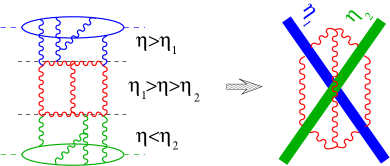
Figure 1: High-energy effective action as an amplitude of the collision of two shock waves.

Due the parton saturation at high energiesGLR ; muchu ; mu90 , the characteristic scale of the transverse momenta in hadron-hadron collisions is $Q_{s}\sim e^{c\eta}$ mu99 ; mabraun ; iancu02 ; tolpa and therefore the collision of QCD shock waves can be treated using semiclassical methods mvmodel . Within the semiclassical approach, the problem of scatering of two shock waves can be reduced to the solution of classical YM equations with sources being the shock waves nncoll (see also prd99 ). At present, these equations have not been solved. There are two approaches discussed in current literature: numerical simulations krasvenu and expansion in the strength of one of the shock waves. The collision of a weak and a strong shock waves corresponds to the deep inelastic scattering from a nucleus (and scattering of two strong shock waves describes a nucleus-nucleus collision). The first term of the expansion of the strength of one of the waves was calculated in a number of papers kovmu99 ; kop ; wkov . Recently, the classical field was calculated up to the second order in a weak source prd04 . I will use some formulas of Ref. prd04 , although the main result for the effective action will be derived independently. The obtained effective action, symmetric with respect to projectile and target, has a “built-in” projectile-target duality (which is a highly nontrivial property of the light-cone Hamiltonian in the framework of the Hamiltonian approachsmith ; larecent ; kl05 ; mu05 ; murecent ). In terms of Feynman diagrams the effective action includes both “up” and “down” fan diagrams and therefore it describes pomeron loops which are a topic of intensive discussion in the current literaturelevin ; smith ; larecent ; kl05 ; mu05 ; murecent .

The paper is organized as follows. Sec. 2 is devoted to the rapidity factorization which is the starting point of the shock-wave approach. In Sect. 3 I define the high-energy effective action as a scattering amplitude of QCD shock waves and develop the expansion in commutators of Wilson lines. In Sec. 4 I find the effective action for a given (infinitesimal) range of rapidity in the leading order in this expansion. The corresponding functional integral over the dynamical Wilson-line variables is constructed in Sec. 5. The explicit form of the first-order classical fields created by the collision of two shock waves is presented in the Appendix.

II Rapidity factorization

The main technical tool of the shock-wave approach to the high-energy scattering is the rapidity factorization developed in prl ; prd99 . Consider a functional integral for the typical scattering amplitude

$$\int\!DAJ(p_{A})J(p_{B})J(-p^{\prime}_{A})J(-p^{\prime}_{B})~{}e^{iS(A)}$$ (1)

where the currents $J(p_{A})$ and $J(p_{B})$ describe the two colliding particles (say, photons).

Throughout the paper, we use Sudakov variables

$$k~{}=~{}\alpha p_{1}+\beta p_{2}+k_{\perp}$$ (2)

and the notations

$$x_{\bullet}=p_{1}^{\mu}x_{\mu}=\sqrt{s\over 2}x^{-},~{}~{}~{}~{}x^{-}={1\over\sqrt{2}}(x^{0}-x^{3})$$

$$x_{\ast}=p_{2}^{\mu}x_{\mu}=\sqrt{s\over 2}x^{+},~{}~{}~{}~{}x^{+}={1\over\sqrt{2}}(x^{0}+x^{3})$$ (3)

Here $p_{1}$ and $p_{2}$ are the light-like vectors close to $p_{A}$ and $p_{B}$: $p_{A}=p_{1}+{p_{A}^{2}\over s}p_{2}$, $p_{B}=p_{2}+{p_{B}^{2}\over s}p_{1}$.

Let us take some “rapidity divide” $\eta_{1}$ such that $\eta_{A}>\eta_{1}>\eta_{B}$ and integrate first over the gluons with the rapidity $\eta>\eta_{1}$, see Fig. 2.

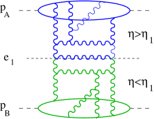
Figure 2: Rapidity factorization.

From the viewpont of such particles, the fields with $\eta<\eta_{1}$ shrink to a shock wave so the result of the integration is presented by Feynman diagrams in the shock-wave background. With the LLA accuracy, in the Feynman integrals over the gluons with $\eta>\eta_{1}$ one can set $\eta_{1}\rightarrow-\infty$ (replace the “rapidity divide” vector $e_{1}=p_{1}+e^{-\eta_{1}}p_{2}$ by the light-like vector $p_{2}$) so the shock wave is infinitely thin and light-like. In the covariant gauge, this shock-wave has the only non-vanishing component $A_{\bullet}$ which is concentrated near $x_{\ast}=0$. In order to write down factorization we need to rewrite the shock wave in the temporal gauge $A_{0}=0$. In such gauge the most general form of a shock-wave background is (see Fig. 3)

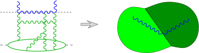
Figure 3: Shock wave in the temporal gauge.

$$A^{i}={\cal U}_{1}^{i}\theta(x_{\ast})+{\cal U}_{2}^{i}\theta(-x_{\ast}),~{}~{}~{}A_{\bullet}=A_{\ast}=0$$ (4)

where

$${\cal U}_{1}^{i}~{}=~{}U_{1}^{\dagger}{i\over g}\partial_{i}U_{1},~{}~{}~{}~{}~{}{\cal U}_{2}^{i}~{}=~{}U_{1}^{\dagger}{i\over g}\partial_{i}U_{2}$$ (5)

are the pure gauge fields (filling the half-spaces $x_{\ast}<0$ and $x_{\ast}<0$ ). There is a redundant gauge symmetry

$$U_{1}(x_{\perp})\rightarrow U_{1}(x_{\perp})\Omega(x_{\perp}),~{}~{}~{}~{}U_{2}(x_{\perp})\rightarrow U_{2}(x_{\perp})\Omega(x_{\perp})$$ (6)

related to the fact that gauge invariant objects like the color dipole

$${\rm Tr}\{[\infty p_{2},-\infty p_{2}]_{x}[x_{\perp}-\infty p_{2},y_{\perp}-\infty p_{2}][-\infty p_{2},\infty p_{2}]_{y}$$

$$\times~{}[y_{\perp}+\infty p_{2},x_{\perp}+\infty p_{2}]\}~{}\simeq~{}{\rm Tr}\{U_{1x}U^{\dagger}_{2x}U_{2y}U^{\dagger}_{1y}\}$$ (7)

depend only on the product $U_{1z}U^{\dagger}_{2z}$. In papers prd99 ; mobzor this symmetry was used to gauge away $U_{2}$ and simplify the shock wave to $A_{i}={\cal U}_{i}\theta(x_{\ast})$ while in Ref. prd04 the opposite case $U_{1}=0$ ($A_{i}={\cal U}_{i}\theta(-x_{\ast})$) was considered. In the present paper we keep this gauge freedom - as we shall see below it simplifies the effective action for the Wilson-line integral.

The generating functional for the Green functions in the Eq. (4) has the form (cf. mobzor )

$$\int\!\!DAJ(p_{A})J(-p^{\prime}_{A})~{}e^{iS(A)+i\!\int\!d^{2}z_{\perp}(0,F_{\ast i},0)^{a}_{z}({\cal U}_{1}^{ai}-{\cal U}_{2}^{ai})_{z}}$$ (8)

where ($F_{ei}\equiv e^{\mu}F_{\mu i}$ etc.)

$$(0,F_{ei},0)_{z}\equiv\!\int_{-\infty}^{\infty}\!\!\!\!du~{}[0,ue]_{z}F_{ei}(ue+z_{\perp})[ue,0]_{z}~{}$$

$$=~{}[0,\infty e]_{z}(i{\partial\over\partial z^{i}}+gA_{i}(\infty e+z_{\perp}))[\infty e,0]_{z}$$ (9)

$$-~{}[0,-\infty e]_{z}(i{\partial\over\partial z^{i}}+gA_{i}(-\infty e+z_{\perp}))[-\infty e,0]_{z}$$

and $(0,F_{\mu i},0)^{a}\equiv 2{\rm tr}~{}t^{a}(0,F_{\mu i},0)$. (Throughout the paper, the sum over the Latin indices $i,j...$ runs over the two transverse components while the sum over Greek indices runs over the four components as usual).

It is easy to see that the functional integral (8) generates Green functions in the Eq. (4) background. Indeed, let us choose the gauge $A_{\ast}=0$ for simplicity. In this gauge, $(0,F_{\ast i},0)^{a}=A_{i}(\infty p_{2}+z_{\perp})-A_{i}(-\infty p_{2}+z_{\perp})$ so the functional integral (8) takes the form

$$\int\!DA~{}J(p_{A})J(-p^{\prime}_{A})$$ (10)

$$\times~{}e^{iS(A)+i\!\int\!d^{2}z_{\perp}(A_{i}(\infty p_{2}+z_{\perp})-A_{i}(-\infty p_{2}+z_{\perp}))^{a}({\cal U}_{1}^{ai}-{\cal U}_{2}^{ai})_{z}}$$

Let us now shift the fields $A_{i}\rightarrow A_{i}+\bar{A}_{i}$ and where $\bar{A}^{i}={\cal U}_{1}^{i}\theta(x_{\ast})+{\cal U}_{2}^{i}\theta(-x_{\ast})$. The only non-zero components of the classical field strength in our case are $F_{\bullet i}=({\cal U}_{1i}-{\cal U}_{2i})\delta({2\over s}x_{\ast})$ so we get

$$S(A+\bar{A})~{}=~{}{2\over s}\!\int d^{4}zD^{i}\bar{F}_{i\bullet}A^{\ast}-{2\over s}\int\!d^{2}z_{\perp}dz_{\bullet}$$

$$\times~{}\left.A^{i}\bar{F}_{\bullet i}\right|^{x_{\ast}=\infty}_{x_{\ast}=-\infty}+{1\over 2}A^{\mu}(\bar{D}^{2}g_{\mu\nu}-2i\bar{F}_{\mu\nu})A^{\nu}+...$$ (11)

In the $A_{\ast}=0$ gauge the first term in the r.h.s. of Eq. (11) vanishes while the second term cancels with the corresponding contribution $\sim-(A_{i}(\infty p_{2}+z_{\perp})-A_{i}(-\infty p_{2}+z_{\perp}))^{a}{\cal U}^{ai}$ coming from the source in Eq. (8). We obtain

$$\int\!DA~{}J(p_{A})J(-p^{\prime}_{A})$$ (12)

$$\times~{}e^{iS(A)+i\!\int\!d^{2}z_{\perp}(A_{i}(\infty p_{2}+z_{\perp})-A_{i}(-\infty p_{2}+z_{\perp}))^{a}({\cal U}_{1}^{ai}-{\cal U}_{2}^{ai})_{z}}$$

$$=~{}\int\!DA~{}J(p_{A})J(-p^{\prime}_{A})e^{{i\over 2}\!\int\!d^{2}zA^{\mu}(\bar{D}^{2}g_{\mu}\nu-2i\bar{F}_{\mu\nu})A^{\nu}}$$

which gives the Green functions in the Eq. (4) background.

To complete the factorization formula one needs to integrate over the remaining fields with rapidities $\eta<\eta_{1}$:

$$\int\!D{\cal A}DA{\cal J}(p_{A}){\cal J}(p_{B})e^{-iS({\cal A})}~{}e^{iS(A)}J(-p_{A})J(-p_{B})$$

$$=~{}\int\!DAJ(p_{A})J(-p^{\prime}_{A})\int\!DBJ(p_{B})J(-p^{\prime}_{B})$$

$$\times~{}e^{iS(A)+iS(B)+i\!\int\!d^{2}z_{\perp}(0,F_{e_{1}i},0)^{a}_{z}(0,G_{e_{1}i},0)^{a}_{z}}$$ (13)

where the Wilson-line operators $(0,F_{e_{{}_{1}}i},0)^{a}_{z}$ and $(0,G_{e_{{}_{1}}i},0)^{a}_{z}$ are the operators (9) made from $A$ and $B$ fields, respectively. As discussed in prl ; prd99 ; mobzor ; baba03 , the slope of Wilson lines is determined by the “rapidity divide” vector $e_{\eta_{1}}=p_{1}+e^{-\eta_{1}}p_{2}$. (From the wiewpoint of $A$ fields, the slope $e_{1}$ can be replaced by $p_{2}$ with power accuracy so we recover the generating functional (8) with $(0,G_{\ast i},0)={\cal U}_{1i}-{\cal U}_{2i}$).

III Scattering of OCD shock waves

III.1 Efffective action as a shock-wave scattering amplitude

In this section we define the scattering of the shock waves using the rapidity factorization developed above. Applying the factorization formula (13) two times, one gets (see Fig. 4):

$$\int\!DA~{}J(p_{A})J(p_{B})J(-p^{\prime}_{A})J(-p^{\prime}_{B})~{}e^{iS(A)}~{}=$$ (14)

$$\int\!DAJ(p_{A})J(-p^{\prime}_{A})e^{iS(A)}\!\int\!DB~{}J(p_{B})J(-p^{\prime}_{B})~{}e^{iS(B)}$$

$$\times\!\int\!DC\exp\Big{[}iS(C)+i\!\int\!d^{2}z_{\perp}\Big{\{}[0,A_{e_{{}_{1}}i},0]^{a}_{z}[0,C_{e_{{}_{1}}i},0]^{a}_{z}$$

$$\hskip 76.82243pt+~{}(0,C_{e_{{}_{2}}i},0)^{a}_{z}(0,B_{e_{{}_{2}}i},0)^{a}_{z}\Big{\}}\Big{]}$$

where the slope is $e_{1}=p_{1}+e^{-\eta_{1}}p_{2}$ for the $[...]$ Wilson lines and $e_{2}=p_{1}+e^{-\eta_{2}}p_{2}$ for the $(...)$ ones.

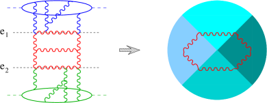
Figure 4: Effective action as a scattering of two shock waves.

The functional integral over the central range of rapidity $\eta_{1}>\eta>\eta_{2}$ is determined by the integral over $C$ field with the sources

$$(0,A_{e_{{}_{1}}i},0)_{z}=[0,\infty e_{{}_{1}}]_{z}(i\partial_{i}+gA_{i}(\infty e_{1}+z_{\perp}))[\infty e_{{}_{1}},0]_{z}$$

$$-~{}[0,-\infty e_{{}_{1}}]_{z}(i\partial_{i}+gA_{i}(-\infty e_{1}+z_{\perp}))[-\infty e_{{}_{1}},0]_{z}$$

$$(0,B_{e_{{}_{2}}i},0)_{z}=[0,\infty e_{{}_{2}}]_{z}(i\partial_{i}+gB_{i}(\infty e_{2}+z_{\perp}))[\infty e_{{}_{2}},0]_{z}$$

$$-~{}[0,-\infty e_{{}_{2}}]_{z}(i\partial_{i}+gB_{i}(-\infty e_{2}+z_{\perp}))[-\infty e_{{}_{2}},0]_{z}$$ (15)

made from “external” $A$ and $B$ fields. Since $A_{i}(\pm\infty)$ is a pure gauge these sources can be represented as a difference of a pure-gauge fields $(0,A_{e_{{}_{1}}i},0)_{z}=({\cal V}_{1}^{ai}-{\cal V}_{2}^{ai})_{z}$ and $(0,B_{e_{{}_{2}}i},0)_{z}=({\cal U}_{1}^{ai}-{\cal U}_{2}^{ai})_{z}$ where

$$V_{1,2}(z_{\perp})=[0,\pm\infty e_{1}]_{z}[\pm\infty e_{1}+z_{\perp},\pm\infty e_{1}+\infty e_{\perp}]$$

$$U_{1,2}(z_{\perp})=[0,\pm\infty e_{2}]_{z}[\pm\infty e_{2}+z_{\perp},\pm\infty e_{2}+\infty e_{\perp}]$$ (16)

Since there is no field strength $F_{\mu\nu}$ at infinite time the direction of $e_{\perp}$ does not matter.

The result of the integration over the $C$ field is an effective action for the $\eta_{1}>\eta>\eta_{2}$ interval of rapidity

$$e^{iS_{\rm eff}(V_{1},V_{2},U_{1},U_{2};\eta_{1}-\eta_{2})}~{}$$ (17)

$$=\int\!\!DC\exp\Big{[}iS(C)+i\!\int\!d^{2}z_{\perp}\Big{\{}({\cal V}_{1}^{ai}-{\cal V}_{2}^{ai})_{z}[0,C_{e_{{}_{1}}i},0]^{a}_{z}$$

$$\hskip 76.82243pt+~{}({\cal U}_{1}^{ai}-{\cal U}_{2}^{ai})_{z}(0,C_{e_{{}_{2}}i},0)^{a}_{z}\Big{\}}\Big{]}.$$

One can interpret Eq. (17) as an effective action for scattering of two QCD shock waves defined by the sources (16). Note that the effective action $iS_{\rm eff}(V_{1},V_{2},U_{1},U_{2};\eta_{1}-\eta_{2})$ defined by Eq. (17) is invariant under the redundant gauge transformations (6)

$$U_{1(2)}(x_{\perp})\rightarrow U_{1(2)}(x_{\perp})\Omega(x_{\perp}),$$

$$V_{1(2)}(x_{\perp})\rightarrow V_{1(2)}(x_{\perp})\Omega^{\prime}(x_{\perp})$$ (18)

since this transformation can be absorbed by a gauge rotation of the $C$ fields

$$C_{\mu}\rightarrow\Omega^{\dagger}(x_{\perp},\ln{x_{\ast}\over x_{\bullet}})C_{\mu}\Omega(x_{\perp},\ln{x_{\ast}\over x_{\bullet}})$$

$$+~{}{i\over g}\Omega^{\dagger}(x_{\perp},\ln{x_{\ast}\over x_{\bullet}})\partial_{\mu}\Omega(x_{\perp},\ln{x_{\ast}\over x_{\bullet}})$$ (19)

where $\Omega(x_{\perp},\ln{x_{\ast}\over x_{\bullet}})$ is an arbitrary $SU_{3}$ matrix satisfying the conditions $\Omega^{\dagger}(x_{\perp},\eta_{1})=\Omega(x_{\perp})$ and $\Omega^{\dagger}(x_{\perp},\eta_{2})=\Omega^{\prime}(x_{\perp})$.

With a power accuracy $O(m^{2}/s)$, we can replace $e_{1}$ by $p_{1}$ and $e_{2}$ by $p_{2}$ :

$$e^{iS_{\rm eff}(V_{1},V_{2},U_{1},U_{2};\eta_{1}-\eta_{2})}~{}$$ (20)

$$=~{}\int\!\!DC\exp\Big{\{}iS(C)+i\!\int\!d^{2}z_{\perp}\Big{[}({\cal V}_{1}^{ai}-{\cal V}_{2}^{ai})_{z}[0,C_{\bullet i},0]^{a}_{z}$$

$$\hskip 85.35826pt+~{}({\cal U}_{1}^{ai}-{\cal U}_{2}^{ai})_{z}(0,C_{\ast i},0)^{a}_{z}\Big{]}\Big{\}}$$

The saddle point of the functional integral (20) is determined by the classical equations

$${\delta\over\delta C_{\mu}^{a}}\Big{\{}S(C)+i\!\int\!d^{2}z_{\perp}\Big{[}({\cal V}_{1}^{ai}-{\cal V}_{2}^{ai})_{z}[0,C_{\bullet i},0]^{a}_{z}$$

$$\hskip 28.45274pt+~{}({\cal U}_{1}^{ai}-{\cal U}_{2}^{ai})_{z}(0,C_{\ast i},0)^{a}_{z}\Big{]}\Big{\}}~{}=~{}0$$ (21)

At present it is not known how to solve this equations (for the numerical approach see krasvenu ). In the next section we will develop a “perturbation theory” in powers of the parameter $[U,V]\sim g^{2}[{\cal U}_{i},{\cal V}_{j}]$. Note that the conventional perturbation theory corresponds to the case when ${\cal U}_{i},{\cal V}_{i}\sim 1$ while the semiclassical QCD is relevant when the fields are large (${\cal U}_{i}$ and/or ${\cal V}_{i}\sim{1\over g}$).

III.2 Expansion in commutators of Wilson lines

The effective action is defined by the functional integral (20) (hereafter we switch back to the usual notation $A_{\mu}$ for the integration variable and $F_{\mu\nu}$ for the field strength)

$$e^{iS_{\rm eff}(V_{1},V_{2},U_{1},U_{2};\eta_{1}-\eta_{2})}~{}$$

$$=~{}\int\!\!DA\exp\Big{(}iS(A)+i\!\int\!d^{2}z_{\perp}\Big{\{}({\cal V}_{1}^{ai}-{\cal V}_{2}^{ai})_{z}[0,F_{\bullet i},0]^{a}_{z}$$

$$+~{}({\cal U}_{1}^{ai}-{\cal U}_{2}^{ai})_{z}(0,F_{\ast i},0)^{a}_{z}\Big{\}}\Big{)}$$ (22)

Taken separately, the sources $\sim{\cal U}_{i}$ create a shock wave ${\cal U}_{1i}\theta(x_{\ast})+{\cal U}_{2i}\theta(-x_{\ast})$ and those $\sim{\cal V}_{i}$ create ${\cal V}_{1i}\theta(x_{\bullet})+{\cal V}_{2i}\theta(-x_{\bullet})$ In QED, the two sources ${\cal U}_{i}$ and ${\cal V}_{i}$ do not interact (in the leading order in $\alpha$) so the sum of the two shock waves

$$\bar{A}_{i}^{(0)}={\cal U}_{1i}\theta(x_{\ast})+{\cal U}_{2i}\theta(-x_{\ast})+{\cal V}_{1i}\theta(x_{\bullet})+{\cal V}_{2i}\theta(-x_{\bullet})~{},$$

$$\bar{A}_{\bullet}^{(0)}=\bar{A}_{\ast}^{(0)}=0$$ (23)

is a classical solution to the set of equations (21). In QCD, the interaction between these two sources is described by the commutator $g[{\cal U}_{i},{\cal V}_{k}]$ (the coupling constant $g$ corresponds to the three-gluon vertex). The straightforward approach is to take the trial configuration in the form of a sum of the two shock waves and expand the “deviation” of the full QCD solution from the QED-type ansatz (23) in powers of commutators $[U,V]$. This is done rigorously in prd04 and the relevant formulas are presented in the Appendix. Here we will use a slightly different zero-order approximation (cf. mobzor ) which leads to same results in a more streamlined way at a price of some uncertainties (like $\theta(0)$) which, however, do not contribute to the effective action in the leading order.

Let us consider the behavior of the solution of the YM equations at, say, $x_{0}\rightarrow\infty$, $x_{3}$ fixed (in the forward quadrant of the space). Since there is no field strength at $t\rightarrow\infty$, the field must be a pure gauge. As demonstrated in Ref. prd04 , this pure-gauge field has the form of a sum of the shock waves plus a correction proportional to their commutator. Technically, for a pair of pure gauge fields ${\cal U}_{i}(x_{\perp})$ and ${\cal V}_{i}(x_{\perp})$ we define ${\cal W}_{i}(x_{\perp})={\cal U}_{i}(x_{\perp})+{\cal V}_{i}(x_{\perp})+gE_{i}(x_{\perp};U,V)$ as a pure gauge field satisfying the equation $(i\partial_{i}+g[{\cal U}_{i}+{\cal V}_{i},)E^{i}=0$. In the first order in $[U,V]$ this field has the form

$$E^{a}_{i}(U,V)~{}=~{}-(x_{\perp}|U{p^{k}\over p_{\perp}^{2}}U^{\dagger}+V{p^{k}\over p_{\perp}^{2}}V^{\dagger}$$

$$-~{}{p^{k}\over p_{\perp}^{2}}|^{ab}[{\cal U}_{i},{\cal V}_{k}]^{b}-i\leftrightarrow k)+O([U,V]^{2})$$ (24)

where $[{\cal U}_{i},{\cal V}_{k}]^{a}\equiv 2{\rm Tr}t^{a}[{\cal U}_{i},{\cal V}_{k}]$. The second, $[U,V]^{2}$, term of the expansion (24) can be found in prd04 but we do not need it with our accuracy.

Throughout the paper, we use Schwinger notations for the propagator in the external field $(x|{1\over P^{2}}|y)$. For the bare propagator it reduces to $(x|{1\over p^{2}}|y)$ and for the two-dimensional propagator in the transverse space we use the notation $(x_{\perp}|{1\over p_{\perp}^{2}}|y_{\perp})$ where $p_{\perp}^{2}=-p_{i}p^{i}$. Also, $|f)$ denotes $\int\!d^{2}z_{\perp}f(z_{\perp})|z_{\perp})$ and later we will use the notation $|0,f)\equiv\int\!d^{2}z_{\perp}f(z_{\perp})|0,z_{\perp})$.

The zero-order approximation for the solution of the classical equations for the functional integral (22) can be taken as a superposition of pure gauge fields in the forward, backward, left, and right quadrants of the space (see Fig. 5):

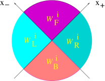
Figure 5: Pure-gauge ansatz as a zero-order approximation to the classical field created by the collision of shock waves.

$$\bar{A}_{\bullet}^{(0)} = \bar{A}_{\ast}^{(0)}=0$$ (25)

$$\bar{A}^{(0)i} = {\cal W}_{F}^{i}(x_{\perp})\theta(x_{\ast})\theta(x_{\bullet})+{\cal W}_{L}^{i}(x_{\perp})\theta(-x_{\ast})\theta(x_{\bullet})$$

$$+ {\cal W}_{R}^{i}(x_{\perp})\theta(x_{\ast})\theta(-x_{\bullet})+{\cal W}_{B}^{i}(x_{\perp})\theta(-x_{\ast})\theta(-x_{\bullet})$$

where

$${\cal W}_{F}^{i}={\cal U}_{1}^{i}+{\cal V}_{1}^{i}+E_{F}^{i},~{}~{}~{}{\cal W}_{L}^{i}={\cal U}_{2}^{i}+{\cal V}_{1}^{i}+E_{F}^{i}$$

$${\cal W}_{R}^{i}={\cal U}_{1}^{i}+{\cal V}_{2}^{i}+E_{F}^{i},~{}~{}~{}{\cal W}_{B}^{i}={\cal U}_{2}^{i}+{\cal V}_{2}^{i}+E_{F}^{i}$$ (26)

and $E_{F}^{i}(U_{1},V_{1})$, $E_{L}^{i}(U_{2},V_{1})$, $E_{R}^{i}(U_{1},V_{2})$, and $E_{B}^{i}(U_{2},V_{2})$ are given by Eq. (24). For the trial configuration (25)

$$\bar{F}_{\bullet}^{~{}i}=\delta({2x_{\ast}\over s})\{\theta(x_{\bullet})({\cal W}_{F}^{i}-{\cal W}_{L}^{i})+\theta(-x_{\bullet})({\cal W}_{R}^{i}-{\cal W}_{B}^{i})\}$$

$$\bar{F}_{\ast}^{~{}i}=\delta({2x_{\bullet}\over s})\{\theta(x_{\ast})({\cal W}_{F}^{i}-{\cal W}_{R}^{i})+\theta(-x_{\ast})({\cal W}_{L}^{i}-{\cal W}_{B}^{i})\}$$

(27)

so

$$D^{i}\bar{F}_{\bullet i} = \delta({2\over s}x_{\ast})\Big{(}[\theta(x_{\bullet})(\partial^{i}-i[\bar{A}^{i},)({\cal W}_{Fi}-{\cal W}_{Li})$$

$$+ \theta(-x_{\bullet})(\partial^{i}-i[\bar{A}^{i},)({\cal W}_{Ri}-{\cal W}_{Bi})$$

$$D^{i}\bar{F}_{\ast i} = \delta({2\over s}x_{\bullet})\Big{(}\theta(x_{\ast})(\partial^{i}-i[\bar{A}^{i},)({\cal W}_{Fi}-{\cal W}_{Ri})$$ (28)

$$+ \theta(-x_{\ast})(\partial^{i}-i[\bar{A}^{i},)({\cal W}_{Li}-{\cal W}_{Bi})$$

and

$$D_{\ast}\bar{F}_{\bullet i}~{}=~{}D_{\ast}\bar{F}_{\bullet i}~{}$$ (29)

$$=~{}\delta({2\over s}x_{\ast})\delta({2\over s}x_{\bullet})({\cal W}_{Fi}-{\cal W}_{Ri}-{\cal W}_{Li}+~{}{\cal W}_{Bi})$$

$$=~{}\delta({2\over s}x_{\ast})\delta({2\over s}x_{\bullet})(E_{Fi}-E_{Ri}-E_{Li}+E_{Bi})$$

Next, one shifts $A\rightarrow A+\bar{A}_{i}^{(0)}$ in the functional integral (22) and obtains

$$e^{iS_{\rm eff}(V_{1},V_{2},U_{1},U_{2};\eta_{1}-\eta_{2})}~{}$$ (30)

$$=~{}\int\!DA~{}\exp\Big{\{}iS(\bar{A})+i\!\int\!d^{4}z({1\over 2}A^{\mu}\bar{D}_{\mu\nu}A^{\nu}+T^{\mu}A_{\mu})\Big{\}}.$$

Here

$$\bar{S}~{}=~{}{1\over 2}\!\int\!d^{2}z_{\perp}\Big{\{}({\cal V}_{1}-{\cal V}_{2})_{i}^{a}({\cal W}_{F}^{i}-{\cal W}_{L}^{i}+{\cal W}_{R}^{i}-{\cal W}_{B}^{i})^{ia}$$

$$~{}+({\cal U}_{1}-{\cal U}_{2})_{i}^{a}({\cal W}_{F}+{\cal W}_{L}-{\cal W}_{R}-{\cal W}_{B})^{ia}-{1\over 2}({\cal W}_{F}$$

$$~{}-{\cal W}_{L}+{\cal W}_{R}-{\cal W}_{B})^{ia}({\cal W}_{F}+{\cal W}_{L}-{\cal W}_{R}-{\cal W}_{B})_{i}^{a}$$ (31)

is a sum of the action and source contributions due to the trial configuration (25), $D_{\mu\nu}=D^{2}(\bar{A})g_{\mu\nu}-2i\bar{F}_{\mu\nu}$ is the inverse propagator in the background-Feynman gauge and $T_{\mu}$ is the linear term for our trial configuration:

$$T_{i} = 2\delta({2\over s}x_{\ast})\delta(x_{\bullet})({\cal W}_{F}^{i}-{\cal W}_{L}^{i}-{\cal W}_{R}^{i}+{\cal W}_{B}^{i})$$

$$= 2\delta({2\over s}x_{\ast})\delta(x_{\bullet})(E_{F}^{i}-E_{L}^{i}-E_{R}^{i}+E_{B}^{i})$$

$$T_{\ast} = -{i\over 2}\delta({2\over s}x_{\bullet})\Big{(}\theta(x_{\ast})[{\cal V}_{1i}-{\cal V}_{2i},E_{F}^{i}+E_{R}^{i}]$$

$$+ \theta(-x_{\ast})[{\cal V}_{1i}-{\cal V}_{2i},E_{L}^{i}+E_{B}^{i}]\Big{)}$$

$$T_{\bullet} = -{i\over 2}\delta({2\over s}x_{\ast})\Big{(}\theta(x_{\bullet})[{\cal U}_{1i}-{\cal U}_{2i},E_{F}^{i}+E_{L}^{i}]$$ (32)

$$+ \theta(-x_{\ast})[{\cal U}_{1i}-{\cal U}_{2i},E_{R}^{i}+E_{B}^{i}]\Big{)}$$

The first line in this equation follows directly from Eq. (29) while the two last lines are obtained by adding Eqs. (28) and the corresponding first derivatives of the sources (21)

$$\left.{\delta\over\delta A_{\ast}}\!\int\!d^{2}z_{\perp}({\cal U}_{1}^{ai}-{\cal U}_{2}^{ai})_{z}(0,F_{\ast i},0)^{a}_{z}\right|_{A_{\ast}=0}$$

$$=~{}\delta(x_{\ast})\Big{\{}[\theta(x_{\bullet})(\partial^{i}-i[\bar{A}^{i}(\infty p_{2}+x_{\perp}),)({\cal U}_{1i}-{\cal U}_{2i})$$

$$+~{}\theta(-x_{\bullet})(\partial^{i}-i[\bar{A}^{i}(-\infty p_{2}+x_{\perp}),)({\cal U}_{1i}-{\cal U}_{2i})\Big{\}}$$

$$\left.{\delta\over\delta A_{\bullet}}\!\int\!d^{2}z_{\perp}\Big{[}({\cal V}_{1}^{ai}-{\cal V}_{2}^{ai})_{z}[0,F_{\bullet i},0]^{a}_{z}\right|_{A_{\bullet}=0}$$

$$=~{}\delta(x_{\bullet})\Big{\{}\theta(x_{\ast})(\partial^{i}-i[\bar{A}^{i}(\infty p_{1}+x_{\perp}),)({\cal V}_{1i}-{\cal V}_{2i})$$

$$+~{}\theta(-x_{\ast})(\partial^{i}-i[\bar{A}^{i}(-\infty p_{1}+x_{\perp}),)({\cal V}_{1i}-{\cal V}_{2i})\}$$ (33)

We get

$$\left.{\delta\over\delta A_{\ast}}\Big{\{}S_{\rm QCD}+\!\int\!d^{2}z_{\perp}({\cal U}_{1}^{ai}-{\cal U}_{2}^{ai})_{z}(0,F_{\ast i},0)^{a}_{z}\Big{\}}\right|_{A_{\ast}=0}$$

$$=~{}-\delta(x_{\ast})\Big{\{}\theta(x_{\bullet})(\partial^{i}-i[\bar{A}^{i}(\infty p_{2}+x_{\perp}),)(E_{Fi}-E_{Li})$$

$$+~{}\theta(-x_{\bullet})(\partial^{i}-i[\bar{A}^{i}(-\infty p_{2}+x_{\perp}),)(E_{Ri}-E_{Bi})\Big{\}},$$

$$\left.{\delta\over\delta A_{\bullet}}\Big{\{}S_{\rm QCD}+\!\int\!d^{2}z_{\perp}\Big{[}({\cal V}_{1}^{ai}-{\cal V}_{2}^{ai})_{z}[0,F_{\bullet i},0]^{a}_{z}\Big{\}}\right|_{A_{\bullet}=0}$$

$$=~{}-\delta(x_{\bullet})\Big{\{}\theta(x_{\ast})(\partial^{i}-i[\bar{A}^{i}(\infty p_{1}+x_{\perp}),)(E_{Fi}-E_{Ri})$$

$$+~{}\theta(-x_{\ast})(\partial^{i}-i[\bar{A}^{i}(-\infty p_{1}+x_{\perp}),)(E_{Li}-E_{Bi})\}$$ (34)

Using $\theta(0)={1\over 2}$ so that $\bar{A}^{i}(\infty p_{2}+x_{\perp})={1\over 2}({\cal W}_{Ri}+{\cal W}_{Bi})$, $\bar{A}^{i}(-\infty p_{2}+x_{\perp})={1\over 2}({\cal W}_{Li}+{\cal W}_{Bi})$, $\bar{A}^{i}(\infty p_{1}+x_{\perp})={1\over 2}({\cal W}_{Fi}+{\cal W}_{Ri})$, $\bar{A}^{i}(-\infty p_{1}+x_{\perp})={1\over 2}({\cal W}_{Li}+{\cal W}_{Bi})$, and the condition $(i\partial_{i}+[{\cal W}_{i},)E^{i}=0$ one easily obtains Eq. (32).

Expansion in powers of $T$ in the functional integral (30) yields the set of Feynman diagrams in the external fields (23) with the sources (32). The parameter of the expansion is $g^{2}[{\cal U}_{i},{\cal V}_{j}]$ ($\sim[U,V]$, see Eq. (5)).

IV The effective action

IV.1 The effective action in the lowest order

The effective action (22) in the first nontrivial order in $[U,V]$ is given by the integration of linear terms (32) with the Green functions in the external field (25)

$$iS_{\rm eff}(U,V)~{}=~{}$$

$$-{1\over 2}\!\int\!d^{4}zd^{4}z^{\prime}T^{a}_{\mu}(z)\langle A^{\mu a}(z)A^{\nu b}(z^{\prime})\rangle T^{b}_{\nu}(z^{\prime})$$ (35)

It is easy to see that the term $\sim T_{\ast}T_{\bullet}$ is $\sim[U,V]^{3}$ so the leading contribution $\sim[U,V]^{2}$ comes from the product of two $T_{i}$’s which has the form

$${i\over 2}\!\int\!d^{2}z_{\perp}d^{2}z^{\prime}_{\perp}L^{a}_{i}(z_{\perp})(0,z_{\perp}|{1\over P^{2}+i\epsilon}|0,z^{\prime}_{\perp})^{ab}L^{bi}(z^{\prime}_{\perp})$$ (36)

where

$$L_{i} \equiv 2(E_{F}^{i}-E_{L}^{i}-E_{R}^{i}+E_{B}^{i})$$ (37)

$$= 2({\cal W}_{F}^{i}-{\cal W}_{L}^{i}-{\cal W}_{R}^{i}+{\cal W}_{B}^{i})$$

is actually the transverse part of the Lipatov vertex of the gluon emission by the scattering of two shock waves in the first order in $[U,V]$ (see Appendix). As we shall see below, the main logarithmic contribution to the integral (36) comes from the region $z_{\perp}\rightarrow z^{\prime}_{\perp}$ where one can replace the propagator in the background field by the bare propagator. One obtains

$$ig^{2}{s\over 2}\!\int\!{d\alpha d\beta\over 8\pi^{2}}(0,L_{i}^{a}|{1\over\alpha\beta s-p^{2}_{\perp}+i\epsilon}|0,L^{ia})$$ (38)

The integral (38) is formally divegrent. Within the LLA accuracy, one can cut the integration off at the width of the shock waves $\lambda\sim\sqrt{s\over m^{2}}e^{-\eta_{1}/2}$, $\rho\sim\sqrt{s\over m^{2}}e^{\eta_{2}/2}$ and obtain:

$$ig^{2}{s\over 2}\!\!\int\!{d\alpha d\beta\over 8\pi^{2}}e^{-i(\alpha\lambda+\beta\rho)}(0,L_{i}^{a}|{1\over\alpha\beta s-p^{2}_{\perp}+i\epsilon}|0,L^{ia})$$

$$=~{}{\alpha_{s}\Delta\eta\over 4}\!\int d^{2}z_{\perp}L_{i}^{a}(z_{\perp})L^{ia}(z_{\perp})$$ (39)

where $\Delta\eta=\eta_{1}-\eta_{2}$ is our rapidity interval.

In addition, within the LLA approximation the zero-order term (31) can be simplified to

$$\bar{S} = \int\!d^{2}z_{\perp}({\cal V}_{1}-{\cal V}_{2})^{ia}({\cal U}_{1}-{\cal U}_{2})_{i}^{a}$$ (40)

Indeed, it is easy to see that in the r.h.s. of Eq. (31) the terms $\sim[U,V]$ cancel while the the terms $\sim[U,V]^{2}$ are not multiplied by $\Delta\eta$ so they can be omitted in the LLA (the Eq. (39) is $\sim[U,V]^{2}\Delta\eta$). It is worth noting that Eq. (40) is the usual light-cone lattice action pirner in the limit when transverse size of the plaquette vanishes and the longitudinal increases to infinity. Thus, the effective action in the first order can be represented as

$$S_{\rm eff}(U,V)~{}=~{}\!\int\!d^{2}z_{\perp}\Big{\{}({\cal V}_{1}-{\cal V}_{2})_{i}^{a}({\cal U}_{1}-{\cal U}_{2})_{i}^{a}$$

$$-~{}i{\alpha_{s}\Delta\eta\over 4}\!\int d^{2}z_{\perp}L_{i}^{a}(z_{\perp})L^{ia}(z_{\perp})\Big{\}}$$ (41)

We shall see below that $L_{i}$ is the Lipatov vertex of the gluon emission by the scattering of two shock waves in the first order in $[U,V]$. Note that $S_{\rm eff}$ given by Eq. (41) is invariant with respect to rotation of the sources

$$U_{j}\rightarrow U_{j}\Omega,~{}~{}~{}~{}V_{j}\rightarrow V_{j}\Omega$$ (42)

For the first term in the r.h.s. of Eq. (41) it is trivial while for the second it follows from the gauge-invariant form discussed in the next section, see Eq. (56).

For future applications we will rewrite the effective action (41) as a Gaussian integration over the auxiliary field $\lambda$ coupled to Lipatov vertex (90):

$$e^{iS_{\rm eff}(U,V)}~{}=~{}e^{i\int d^{2}z_{\perp}~{}({\cal V}_{1}-{\cal V}_{2})^{ia}({\cal U}_{1}-{\cal U}_{2})_{i}^{a}}$$ (43)

$$\times~{}\int D\lambda\exp\Big{\{}-\alpha_{s}\Delta\eta\int\!d^{2}z_{\perp}(\lambda^{a}_{i}\lambda^{ai}-L^{a}_{i}\lambda^{ai})\Big{\}}$$

IV.2 Nonlinear evolution equation from the effective action

Let us prove now that the effective action (43) agrees with the non-linear evolution equation. To find the evolution of the dipole $U_{x}U^{\dagger}_{y}$, we need to consider the effective action for the weak source $V$. From eq. (24) one sees that at small $g{\cal V}_{i}\sim\partial_{i}V$

$$L^{a}_{i}(x_{\perp})=-2(x|U_{1}^{\dagger}{p_{i}p^{k}\over p_{\perp}^{2}}U_{1}-U_{2}^{\dagger}{p_{i}p^{k}\over p_{\perp}^{2}}U_{2}|^{ab}({\cal V}_{1}-{\cal V}_{2})^{b}_{k})$$ (44)

and Eq. (22) can be rewritten as

$$\int\!\!DA\exp\Big{\{}iS(A)+i\!\int\!d^{2}z_{\perp}\Big{[}({\cal V}_{1}^{ai}-{\cal V}_{2}^{ai})_{z}[0,F_{\bullet i},0]^{a}_{z}$$

$$+~{}({\cal U}_{1}^{ai}-{\cal U}_{2}^{ai})_{z}(0,F_{\ast i},0)^{a}_{z}\Big{]}\Big{\}}$$

$$=\int D\lambda e^{\int\!d^{2}z_{\perp}\{-\alpha_{s}\Delta\eta\lambda^{a}_{i}\lambda^{ai}+i({\cal V}_{1}-{\cal V}_{2})_{i}^{a}(\tilde{{\cal U}}_{1}^{i}-\tilde{{\cal U}}_{2}^{i})^{a}\}}.$$ (45)

Here

$$\tilde{U}_{1} = e^{2\alpha_{s}\Delta\eta{\partial_{i}\over\partial_{\perp}^{2}}(U_{1}\lambda^{i}U_{1}^{\dagger})}U_{1},$$ (46)

$$\tilde{U}_{2} = e^{2\alpha_{s}\Delta\eta{\partial_{i}\over\partial_{\perp}^{2}}(U_{2}\lambda^{i}U_{2}^{\dagger})}U_{2}$$ (47)

so that

$$\tilde{{\cal U}}_{1i}^{a}~{} = ~{}{\cal U}_{1i}^{a}+2\alpha_{s}\Delta\eta(U_{1}^{\dagger}{\partial_{i}\partial^{k}\over\partial_{\perp}^{2}}U_{1})^{ab}\lambda^{b}_{k}$$ (48)

$$\tilde{{\cal U}}_{2i}^{a}~{} = ~{}{\cal U}_{2i}^{a}+2\alpha_{s}\Delta\eta(U_{2}^{\dagger}{\partial_{i}\partial^{k}\over\partial_{\perp}^{2}}U_{2})^{ab}\lambda^{b}_{k}$$ (49)

where we need only the first term in expansion in $\lambda_{i}$ in $\lambda$.

To find the evolution of the color dipole (7) we should expand Eq. (45) in powers of ${\cal V}_{1i}-{\cal V}_{2i}$ and use the formula

$$[0,\infty p_{1}]_{x}[x_{\perp}+\infty p_{1},y_{\perp}+\infty p_{1}][\infty p_{1},0]_{y}^{\eta_{2}}$$

$$=~{}Pe^{ig\!\int_{x}^{y}\!dz_{i}[0,F_{\bullet i},0]_{z}}$$ (50)

which results in

$$U^{\dagger}_{1y}U_{1x}U_{2x}^{\dagger}U_{2y}$$

$$~{}=\int D\lambda~{}e^{-\alpha_{s}\Delta\eta\int\!d^{2}z_{\perp}\lambda^{a}_{i}\lambda^{ai}}~{}\tilde{U}_{1y}^{\dagger}\tilde{U}_{1x}\tilde{U}_{2x}^{\dagger}\tilde{U}_{2y}$$ (51)

Performing the Gaussian integration over $\lambda$ one obtains after some algebra

$${\rm tr}\{U_{1x}U_{2x}^{\dagger}U_{2y}U^{\dagger}_{1y}\}$$ (52)

$$=~{}{\rm tr}\{U_{1x}U_{2x}^{\dagger}U_{2y}U^{\dagger}_{1y}\}+{\alpha_{s}\Delta\eta\over 4\pi^{2}}\!\int\!d^{2}z_{\perp}{(x-y)_{\perp}^{2}\over(x-z)_{\perp}^{2}(z-y)_{\perp}^{2}}$$

$$\times~{}({\rm tr}\{U_{1x}U_{2x}^{\dagger}U_{2z}U^{\dagger}_{1z}\}{\rm tr}\{U_{1z}U_{2z}^{\dagger}U_{2y}U^{\dagger}_{1y}\}$$

$$\hskip 113.81102pt-N_{c}{\rm tr}\{U_{1x}U_{2x}^{\dagger}U_{2y}U^{\dagger}_{1y}\})$$

which is the non-linear evolution equation npb96 ; yura for the Wilson-line operator $U_{x}=U_{1x}U_{2x}^{\dagger}=[\infty e,-\infty e]_{x}$.

IV.3 Gauge-invariant representation of the first-order effective action $L_{i}L^{i}$

Our expression for the $\Delta\eta$ term in the effective action, proportional to the square of the Lipatov vertex $({\cal W}_{F}^{i}-{\cal W}_{L}^{i}-{\cal W}_{R}^{i}+{\cal W}_{B}^{i})^{a}$, was obtained in the axial-type gauges. It can be rewritten it in the gauge-invariant “diamond” form of trace of four Wilson lines at $x_{\bullet,\ast}=\pm\infty$ (see Fig. 6) as suggested in a recent paper smith .

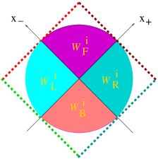
Figure 6: Gauge-invariant form of the effective action.

The “diamond” Wilson loop is defined as follows

$$\Diamond(x_{\perp})\equiv~{}{\rm tr}\{[-\infty p_{1},F_{\bullet i},\infty p_{1}]_{\infty p_{2}}[\infty p_{2},F_{\ast i},-\infty p_{2}]_{\infty p_{1}}$$

$$\hskip 8.53581pt\times~{}[\infty p_{1},-\infty p_{1}]_{-\infty p_{2}}[-\infty p_{2},\infty p_{2}]_{-\infty p_{1}}$$

$$\hskip 8.53581pt+~{}{\rm tr}[-\infty p_{1},\infty p_{1}]_{\infty p_{2}}[\infty p_{2},F_{\ast i},-\infty p_{2}]_{\infty p_{1}}$$

$$\hskip 8.53581pt\times~{}[\infty p_{1},F_{\bullet i},-\infty p_{1}]_{-\infty p_{2}}[-\infty p_{2},\infty p_{2}]_{-\infty p_{1}}$$

$$\hskip 8.53581pt+~{}{\rm tr}[-\infty p_{1},\infty p_{1}]_{\infty p_{2}}[\infty p_{2},-\infty p_{2}]_{\infty p_{1}}$$

$$\hskip 8.53581pt\times~{}[\infty p_{1},F_{\bullet i},\-\infty p_{1}]_{-\infty p_{2}}[-\infty p_{2},F_{\ast i},\infty p_{2}]_{-\infty p_{1}}$$

$$\hskip 8.53581pt+~{}{\rm tr}[-\infty p_{1},F_{\bullet i},\infty p_{1}]_{\infty p_{2}}[\infty p_{2},-\infty p_{2}]_{\infty p_{1}}$$

$$\hskip 8.53581pt\times~{}[\infty p_{1},-\infty p_{1}]_{-\infty p_{2}}[-\infty p_{2},F_{\ast i},\infty p_{2}]_{-\infty p_{1}}\}$$ (53)

where the transverse arguments in all Wilson lines are $x_{\perp}$. Next, define this “diamond” as a function of the sources

$$\Diamond(U_{1},U_{2},V_{1},V_{2})~{}\equiv~{}$$ (54)

$${\cal N}^{-1}\!\int\!\!DA~{}\Diamond(A)~{}\exp\Big{(}iS(A)+i\!\int\!d^{2}z_{\perp}\Big{\{}({\cal V}_{1}^{ai}-{\cal V}_{2}^{ai})_{z}$$

$$\hskip 36.98857pt\times~{}[0,F_{e_{1}i},0]^{a}_{z}+({\cal U}_{1}^{ai}-{\cal U}_{2}^{ai})_{z}(0,F_{e_{2}i},0)^{a}_{z}\Big{\}}\Big{)}$$

(In the Appendix we demonstrate that the trace of four Wilson lines

$${\rm tr}\{[-\infty e_{1},\infty e_{1}]_{\infty e_{2}}[\infty e_{2},-\infty e_{2}]_{\infty e_{1}}$$

$$\times~{}[\infty e_{1},-\infty e_{1}]_{-\infty e_{2}}[-\infty e_{2},\infty e_{2}]_{-\infty e_{1}}\}~{}=~{}1$$ (55)

is trivial in the leading order.)

Note that $\Diamond(U,V)$ is invariant with respect to the rotation of all sources by one gauge matrix $\Omega(x_{\perp})$

$$\Diamond(U_{1}\Omega,U_{2}\Omega,V_{1}\Omega,V_{2}\Omega)=\Diamond(U_{1},U_{2},V_{1},V_{2})$$ (56)

since it can be absorbed by gauge transformation of the fields $A_{\mu}\rightarrow\Omega^{\dagger}A_{\mu}\Omega+{i\over g}\Omega^{\dagger}\partial_{\mu}\Omega$ in the functional integral Eq. (54).

Now we can prove that the square of Lipatov vertex can be expressed as the “diamond” Wilson loop:

$${1\over 4}L^{a}_{i}(U,V)L^{ai}(U,V)~{}=~{}\Diamond(U,V)$$ (57)

Indeed, it is easy to see that for the trial configuration (25) the Eq. (53) reduces to

$$({\cal W}_{Fi}-{\cal W}_{Li})^{a}({\cal W}_{F}^{i}-{\cal W}_{R}^{i})^{a}+({\cal W}_{Ri}-{\cal W}_{Fi})^{a}$$

$$\times~{}({\cal W}_{R}^{i}-{\cal W}_{B}^{i})^{a}+({\cal W}_{Bi}-{\cal W}_{Ri})^{a}({\cal W}_{B}^{i}-{\cal W}_{L}^{i})^{a}$$

$$+~{}({\cal W}_{Li}-{\cal W}_{Bi})^{a}({\cal W}_{L}^{i}-{\cal W}_{F}^{i})^{a}~{}=$$

$$({\cal W}_{Fi}-{\cal W}_{Li}-{\cal W}_{R}^{i}+{\cal W}_{Bi})^{a}({\cal W}_{F}^{i}-{\cal W}_{L}^{i}-{\cal W}_{R}^{I}+{\cal W}_{B}^{i})^{a}$$

which coincide with the l.h.s. of the Eq. (57). In the covariant-type gauges where $A_{i}\rightarrow 0$ as $x_{\parallel}\rightarrow\infty$ the r.h.s of the Eq. (53) can be rewritten as

$$\partial_{i}M_{1}\partial^{i}M_{2}M_{3}^{\dagger}M_{4}^{\dagger}+M_{1}\partial_{i}M_{2}\partial^{i}M_{3}^{\dagger}M_{4}^{\dagger}$$

$$M_{1}M_{2}\partial_{i}M_{3}^{\dagger}\partial_{i}M_{4}^{\dagger}+\partial_{i}M_{1}M_{2}M_{3}^{\dagger}\partial_{i}M_{4}^{\dagger}$$ (58)

where $M_{1}=[-\infty p_{1},\infty p_{1}]_{\infty p_{2}}$, $M_{2}=[\infty p_{2},-\infty p_{2}]_{\infty p_{1}}$, $M_{3}=[\infty p_{1},-\infty p_{1}]_{-\infty p_{2}}$, and $M_{4}=[-\infty p_{2},\infty p_{2}]_{-\infty p_{1}}$. Eq. (58) is the expression obtained recently in smith in the framework of the Hamiltonian approach (see also kl05 ; mu05 ). The corresponding form of our effective action is the following:

$${1\over 4}L^{a}_{i}(U,V)L^{ai}(U,V)~{}$$

$$=~{}\partial_{i}(W_{L}W^{\dagger}_{F})\partial^{i}(W_{F}W^{\dagger}_{R})W_{R}W^{\dagger}_{B}W_{B}W^{\dagger}_{L}$$

$$+~{}W_{L}W^{\dagger}_{F}\partial^{i}(W_{F}W^{\dagger}_{R})\partial_{i}(W_{R}W^{\dagger}_{B})W_{B}W^{\dagger}_{L}$$

$$+~{}W_{L}W^{\dagger}_{F}W_{F}W^{\dagger}_{R}\partial_{i}(W_{R}W^{\dagger}_{B})\partial^{i}(W_{B}W^{\dagger}_{L})$$

$$+~{}\partial_{i}(W_{L}W^{\dagger}_{F})W_{F}W^{\dagger}_{R}W_{R}W^{\dagger}_{B}\partial^{i}(W_{B}W^{\dagger}_{L})$$ (59)

The Eq. (57) links the representation in terms of the effective degrees of freedom (Wilson lines in our case) with the representation in terms of gluons of the underlying Yang-Mills theory via Eq. (54). The remarkable feature of the gauge-invariant form (57) is its universality - if one writes the effective action in terms of some other degrees of freedom (say, reggeized gluons leffaction ) one should recover Eq. (57) once these new effective degrees of freedom are expressed in terms of gluons.

V Functional integral over the dynamical Wilson lines

V.1 Effective action as the integral over the Wilson lines

In this section we will rewrite the functional integral for the effective action (22) in terms of Wilson-line variables. To this end, let us use the factorization formula (13) $n$ times as shown in Fig. 7.

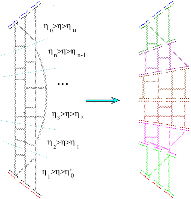
Figure 7: Effective action factorized in $n$ functional integrals.

The effective action factorizes then into a product of $n$ independent functional integrals over the gluon fields labeled by index $k$:

$$e^{iS_{\rm eff}(U,V;\eta)}=$$ (60)

$$\int\!DA^{1}DA^{2}\ldots DA^{n+1}\exp i\Big{\{}({\cal V}_{1}^{i}-{\cal V}_{2}^{i})({\cal U}^{n+1}_{1i}-{\cal U}^{n+1}_{2i})$$

$$+~{}S(A_{n+1})+~{}({\cal V}_{1}^{n+1,i}-{\cal V}_{2}^{n+1,i})({\cal U}^{ni}_{1}-{\cal U}^{ni}_{2})$$

$$+~{}S(A_{n})+\ldots+({\cal V}_{1}^{2i}-{\cal V}_{2}^{2i})({\cal U}_{1i}^{1}-{\cal U}_{2i}^{1})+S(A_{1})$$

$$\hskip 62.59605pt+~{}({\cal V}_{1}^{1i}-{\cal V}_{2}^{1i})({\cal U}_{1i}-{\cal U}_{1i})\Big{\}}~{},$$

where the integrals over $x_{\perp}$ and summation over the color indices are implied. As usually, ${\cal U}^{k,i}_{j}={i\over g}U^{\dagger k}_{j}\partial^{i}U^{k}_{j}$ and ${\cal V}^{k,i}_{j}={i\over g}V^{\dagger k}_{j}\partial^{i}V_{j}^{k}$ where

$$U^{k}_{1(2)}(x_{\perp}) = Pe^{ig\int_{0}^{\pm\infty}du\ n_{k}^{\mu}A_{k,\mu}(un^{k}+x_{\perp})},$$

$$V^{k}_{1(2)}(x_{\perp}) = Pe^{ig\int_{0}^{\pm\infty}du\ n_{k-1}^{\mu}A_{k,\mu}(un^{k-1}+x_{\perp})}$$ (61)

and the vectors $n_{k}$ are ordered in rapidity: $\eta_{0}>\eta_{n}>\eta_{n-1}\ldots\eta_{2}>\eta_{1}>\eta^{\prime}_{0}$. To disentangle integrations over different $A^{k}$, we rewrite $\exp[i({\cal V}_{1}^{k+1,i}-{\cal V}_{2}^{k+1,i})({\cal U}^{k,i}_{1}-{\cal U}^{k,i}_{2})]$ at each “rapidity divide” $\eta_{k}$ as an integral over the auxiliary group variables $\hat{V}^{k+1}_{1,2}$ and $\hat{U}^{k}_{1,2}$ using the formula

$$e^{i\int dx_{\perp}V_{i}U^{i}}~{}=~{}\det(\partial_{i}-ig{\cal V}_{i})(\partial^{i}-ig{\cal U}^{i})$$ (62)

$$\times\int\!D\hat{V}(x_{\perp})D\hat{U}(x_{\perp})e^{i\int dx_{\perp}{\cal V}_{i}\hat{\cal U}^{i}+i\int\!dx_{\perp}\hat{\cal V}_{i}{\cal U}^{i}-i\int dx_{\perp}\hat{\cal V}_{i}\hat{\cal U}^{i}}.$$

(where $\hat{\cal V}_{i}\equiv\hat{V}^{\dagger}{i\over g}\partial_{i}\hat{V}$ and $\hat{\cal U}_{i}\equiv\hat{U}^{\dagger}{i\over g}\partial_{i}\hat{U}$). The determinant gives the perturbative non-logarithmic corrections of the same order as the corrections to the factorization formula (13). In the LLA they can be ignored, consequently, we obtain

$$e^{iS_{\rm eff}(U_{1},U_{2},V_{1},V_{2},\eta_{1}-\eta_{2})}~{}$$ (63)

$$=~{}\int\!\Pi_{k=0}^{n+1}DA^{k}~{}\Pi_{k=0}^{n}D\hat{U}_{1}^{k}D\hat{U}_{2}^{k}D\hat{V}_{1}^{k}D\hat{V}_{2}^{k}$$

$$\times~{}\exp i\Big{\{}({\cal V}_{1}^{i}-{\cal V}_{2}^{i})({\cal U}^{n+1}_{1i}-{\cal U}^{n+1}_{1i})+S(A^{n+1})+({\cal V}_{1i}^{n+1}$$

$$-~{}{\cal V}_{2i}^{n+1})(\hat{\cal U}_{1}^{ni}-\hat{\cal U}_{2}^{ni})-(\hat{\cal V}^{n}_{1i}-\hat{\cal V}^{n}_{2i})(\hat{\cal U}^{n,i}_{1}-\hat{\cal U}^{n,i}_{2})+\ldots$$

$$+~{}({\cal V}_{1i}^{3}-{\cal V}_{2i}^{3})(\hat{\cal U}^{2i}_{1}-\hat{\cal U}^{2i}_{2})-(\hat{\cal V}_{1}^{2i}-\hat{\cal V}_{2}^{2i})(\hat{\cal U}^{2}_{1i}-\hat{\cal U}^{2}_{2i})$$

$$+~{}(\hat{\cal V}^{2}_{2i}-\hat{\cal V}^{2}_{1i})({\cal U}^{2i}_{1}-{\cal U}^{2i}_{2})+S(A^{2})+({\cal V}^{2}_{1i}-{\cal V}^{2}_{2i})(\hat{\cal U}_{1}^{1i}$$

$$-~{}\hat{\cal U}_{2}^{1i})-(\hat{\cal V}^{1}_{1i}-\hat{\cal V}^{1}_{2i})(\hat{\cal U}_{1}^{1i}-\hat{\cal U}_{2}^{1i})+(\hat{\cal V}^{1}_{1i}-\hat{\cal V}^{1}_{2i})$$

$$\hskip 8.53581pt\times~{}({\cal U}^{1i}_{1}-{\cal U}^{1i}_{2})+S(A^{1})+({\cal V}_{1}^{1i}-{\cal V}_{2}^{1i})(U_{1i}-U_{2i})\Big{\}}.$$

Now we can integrate over the gluon fields $A_{k}$. Using the results of the previous Section, we get

$$\int\!DA_{k}\exp\{i(\hat{\cal V}^{k}_{1i}-\hat{\cal V}^{k}_{2i})({\cal U}_{1}^{k,i}-{\cal U}_{2}^{k,i})+iS(A_{k})$$

$$\hskip 34.1433pt+~{}i({\cal V}^{k}_{1i}-{\cal V}^{k}_{2i})(\hat{\cal U}^{k-1,i}_{1}-\hat{\cal U}^{k-1,i}_{2})\}$$

$$\hskip 62.59605pt=~{}e^{iS_{\rm eff}(\hat{V}_{1}^{k},\hat{V}_{2}^{k},\hat{U}_{1}^{k-1},\hat{U}_{2}^{k-1};\Delta\eta)}$$ (64)

where at sufficiently small $\Delta\eta$

$$S_{\rm eff}(\hat{V}_{1}^{k},\hat{V}_{2}^{k},\hat{U}_{1}^{k-1},\hat{U}_{2}^{k-1};\Delta\eta)~{}=~{}(\hat{\cal V}^{k}_{1i}-\hat{\cal V}^{k}_{2i})(\hat{\cal U}^{k-1,i}_{1}$$

$$-~{}\hat{\cal U}^{k-1,i}_{2})~{}-~{}i{\alpha_{s}\Delta\eta\over 4}L_{i}(\hat{\cal V}^{k},\hat{\cal U}_{k-1})L^{i}(\hat{\cal V}^{k},\hat{\cal U}_{k-1})$$ (65)

Performing the integrations over $A^{k}$ we get

$$e^{iS_{\rm eff}(U,V,\eta_{1}-\eta_{2})}~{}=~{}\int\Pi_{k=0}^{n}D\hat{U}_{1}^{k}D\hat{U}_{2}^{k}D\hat{V}_{1}^{k}D\hat{V}_{2}^{k}$$

$$\times~{}\exp i\Big{\{}({\cal V}_{1}^{i}-{\cal V}_{2}^{i})(\hat{\cal U}_{1i}^{n}-\hat{\cal U}_{2i}^{n})-{i\alpha_{s}\over 4}L^{2}(V,\hat{U}^{n})\Delta\eta$$

$$-~{}(\hat{\cal V}^{n}_{1i}-\hat{\cal V}^{n}_{2i})(\hat{\cal U}^{n,i}_{1}-\hat{\cal U}^{n,i}_{2})+\ldots$$

$$-~{}(\hat{\cal V}_{1}^{2i}-\hat{\cal V}_{2}^{2i})(\hat{\cal U}^{2}_{1i}-\hat{\cal U}^{2}_{2i})+(\hat{\cal V}^{2}_{1i}-\hat{\cal V}^{2}_{2i})(\hat{\cal U}_{1}^{1i}-\hat{\cal U}_{2}^{1i})$$

$$-~{}{i\alpha_{s}\over 4}L^{2}(\hat{V}^{2},\hat{U}^{1})\Delta\eta-(\hat{\cal V}^{1}_{1i}-\hat{\cal V}^{1}_{2i})(\hat{\cal U}_{1}^{1i}-\hat{\cal U}_{2}^{1i})$$

$$+~{}(\hat{\cal V}^{1}_{1i}-\hat{\cal V}^{1}_{2i})(U_{1i}-U_{2i})-{i\alpha_{s}\over 4}L^{2}(\hat{V}^{1},U)\Delta\eta\Big{\}}.$$ (66)

In the continuum limit $n\rightarrow\infty$ we obtain the following functional integral for the effective action

$$e^{iS_{\rm eff}(U_{1}(x),U_{2}(x),V_{1}(x),V_{2}(x);\eta_{1}-\eta_{2})}$$ (67)

$$=~{}\left.\int\!\Pi_{j=1,2}DV_{j}(x,\eta)DU_{j}(x,\eta)\right|_{U_{j}(x,\eta_{2})=U_{j}(x)}$$

$$\times~{}\exp\Bigg{[}\int\!d^{2}x\Big{(}i[{\cal V}^{a}_{1i}(x)-{\cal V}^{a}_{2i}(x)][{\cal U}_{1}^{ai}(x,\eta)-{\cal U}_{2}^{ai}(x,\eta)]$$

$$+~{}\int_{\eta^{\prime}_{0}}^{\eta_{0}}\!\!d\eta\Big{\{}-i[{\cal V}^{a}_{1i}(x,\eta)-{\cal V}^{a}_{2i}(x,\eta)]$$

$$\hskip 91.04881pt\times~{}{\partial\over\partial\eta}[{\cal U}_{1}^{ai}(x,\eta)-{\cal U}_{2}^{ai}(x,\eta)]$$

$$+~{}{\alpha_{s}\over 4}L^{a}_{i}(V(x,\eta),U(x,\eta))L^{ai}(V(x,\eta),U(x,\eta))\Big{\}}\Big{)}\Bigg{]}$$

where we displayed the color indices explicitly and removed the hat from the notation of the integration variables. This looks like the functional integral over the canonical coordinates $U$ and canonical momenta $V$ with the (non-local) Hamiltonian $L^{2}(V,U)$. The rapidity $\eta$ serves as the time variable for this system. The above representation of the effective action as an integral over the dynamical Wilson-line variables is the main result of this paper.

Note that the $L_{i}L^{i}$ term in the exponent in (67) is invariant under the rotations (18)

$$U_{j}(x,\eta)\rightarrow U_{j}(x,\eta)\Omega(x,\eta),~{}~{}~{}V_{j}(x,\eta)\rightarrow V_{j}(x,\eta)\Omega(x,\eta)$$ (68)

(see. Eq. (56)), but the term $\sim{\cal U}{\partial\over\partial\eta}{\cal V}$ preserves only the $\eta$-independent symmetry

$$U_{j}(x,\eta)\rightarrow U_{j}(x,\eta)\Omega(x),~{}~{}~{}V_{j}(x,\eta)\rightarrow V_{j}(x,\eta)\Omega(x).$$ (69)

This probably means that the term $\sim{\cal U}{\partial\over\partial\eta}{\cal V}$ should be adjusted by a $\sim[U,V]^{2}$ correction (not important in the LLA) so that the full symmetry (68) is restored.

The idea how to use the factorization formula to rewrite the functional integral in terms of Wilson lines was formulated in Ref. mobzor where the first-order effective action was obtained (the expression in terms of square of Lipatov vertex is given in prd04 ). However, the additional redundant gauge symmetry (18) was fixed by the requirement that there is no field at $t\rightarrow-\infty$ which correspond to the choice $U_{2}=0$ and $V_{2}=0$ for the two colliding shock waves. In this case, one obtains the functional integral in terms of only two variables, $U$ and $V$, at a price of a more complicated form of the effective action mobzor .

It should be noted that $L_{i}^{2}(U,V)$ is only the first term of the expansion of the true high-energy effective action $K(U,V)$ in powers of $[U,V]$. An example of the next-order, $\sim[U,V]^{3}$, contribution to $K(V,U)$ which is missing in the effective action (67) is presented in Ref mobzor, , see Fig. 8.

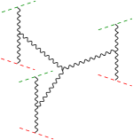
Figure 8: Feynman diagram for a typical $[U,V]^{3}$ term.

V.2 Functional integral for the non-linear evolution

It is instructive do demonstrate that the functional integral (67) reproduces the non-linear evolution in the case of one small source. Basically, we recast the arguments of the Sect. IV.2 in the language of functional integrals.

First, note that at small $V$ the functional integral over ${\cal V}$ is Gaussian (see the Eq. (44)). It is convenient to introduce the “gaussian noise” associated with the Lipatov vertex and rewrite the functional integral (67) as:

$$e^{iS_{\rm eff}(U_{1}(x),U_{2}(x),V_{1}(x),V_{2}(x);\eta_{1}-\eta_{2})}$$ (70)

$$=\left.\int\!\Pi_{j=1,2}DV_{j}(x,\eta)DU_{j}(x,\eta)\right|_{U_{j}(x,\eta_{2})=U_{j}(x)}\!\!D\lambda^{a}_{i}(x,\eta)$$

$$\times~{}\exp\int\!d^{2}x\Big{(}i[{\cal V}^{a}_{1i}(x)-{\cal V}^{a}_{2i}(x)][{\cal U}_{1}^{ai}(x,\eta)-{\cal U}_{2}^{ai}(x,\eta)]$$

$$+~{}\int_{\eta^{\prime}_{0}}^{\eta_{0}}\!\!d\eta\Big{\{}-\alpha_{s}\lambda^{a}_{i}(x,\eta)\lambda^{ai}(x,\eta)$$

$$-~{}i[{\cal V}^{a}_{1i}(x,\eta)-{\cal V}^{a}_{2i}(x,\eta)]{\partial\over\partial\eta}[{\cal U}_{1}^{ai}(x,\eta)-{\cal U}_{2}^{ai}(x,\eta)]$$

$$-~{}2\alpha_{s}\lambda^{ai}(x,\eta)(x|U_{1}^{\dagger}{p_{i}p^{k}\over p_{\perp}^{2}}U_{1}-(1\leftrightarrow 2)|^{ab}({\cal V}^{\eta}_{1}-{\cal V}^{\eta}_{2})^{b}_{k})\Big{\}}\Big{)}.$$

(When convenient, we use the notation $(...)^{\eta}\equiv(...)(\eta)$ for brevity). The integral over ${\cal V}$ gives the $\delta$-function of the form

$$\delta(\partial_{i}({\partial\over\partial\eta}[{\cal U}_{1}^{ai}(x,\eta)-{\cal U}_{2}^{ai}(x,\eta)]$$

$$-~{}2i\alpha_{s}(x|U_{1}^{\dagger}{p_{i}p^{k}\over p_{\perp}^{2}}U_{1}-U_{2}^{\dagger}{p_{i}p^{k}\over p_{\perp}^{2}}U_{2}|^{ab}\lambda^{b\eta}_{k})$$

which restricts $U$ in a following way

$${\partial\over\partial\eta}[{\cal U}_{1}^{ai}(x,\eta)-{\cal U}_{2}^{ai}(x,\eta)]~{}$$

$$\hskip 8.53581pt=~{}2i\alpha_{s}(x|U_{1}^{\dagger}{p_{i}p^{k}\over p_{\perp}^{2}}U_{1}-U_{2}^{\dagger}{p_{i}p^{k}\over p_{\perp}^{2}}U_{2}|^{ab}\lambda_{k}^{b\eta})$$ (71)

It is convenient to rewrite Eq. (71) in the integral form (cf. Eq. 47):

$$U_{i}(x,\eta)=Te^{2i\alpha_{s}t^{a}\!\int_{\eta_{2}}^{\eta}\!d\eta^{\prime}(x|{p^{k}\over p_{\perp}^{2}}U_{i}(\eta^{\prime})^{ab}|\lambda_{k}^{b}(\eta^{\prime}))}U_{i}(x_{\perp},\eta_{2})$$ (72)

where $T$ means ordering in rapidity (= our “time”). The remaining integral over $\lambda$ is gaussian with the “propagator”

$$\langle\lambda_{i}^{a}(x_{\perp},\eta)\lambda_{j}^{b}(y_{\perp},\eta^{\prime})\rangle=g_{ij}\delta^{ab}{1\over 2\alpha_{s}}\delta(x_{\perp}-y_{\perp})\delta(\eta-\eta^{\prime}).$$ (73)

The evolution of the dipole can be represented as

$$U_{1y}^{\dagger\eta}U_{1x}^{\eta}U_{2x}^{\dagger\eta}U_{2y}^{\eta}~{}=\int D\lambda~{}e^{-\alpha_{s}\!\int_{\eta_{2}}^{\eta_{1}}\!d\eta\int\!d^{2}z_{\perp}\lambda^{a\eta}_{iz}\lambda^{ai\eta}_{z}}~{}$$

$$\times~{}U_{1y}^{\dagger\eta_{2}}\bar{T}e^{-2i\alpha_{s}t^{a}\!\int_{\eta_{2}}^{\eta}\!d\eta^{\prime}(y|{p^{k}\over p_{\perp}^{2}}U_{1}^{\eta^{\prime}}|^{ab}\lambda_{k}^{b\eta^{\prime}})}$$

$$\hskip 42.67912pt\times~{}Te^{2i\alpha_{s}t^{a}\!\int_{\eta_{2}}^{\eta}\!d\eta^{\prime}(x|{p^{k}\over p_{\perp}^{2}}U_{1}^{\eta^{\prime}}|^{ab}\lambda_{k}^{b\eta^{\prime}})}U_{1x}^{\eta_{2}}$$

$$\times~{}U_{2x}^{\dagger\eta_{2}}\bar{T}e^{-2i\alpha_{s}t^{a}\!\int_{\eta_{2}}^{\eta}\!d\eta^{\prime}(x|{p^{k}\over p_{\perp}^{2}}U_{2}^{\eta^{\prime}}|^{ab}\lambda_{k}^{b\eta^{\prime}})}$$

$$\hskip 42.67912pt\times~{}Te^{2i\alpha_{s}t^{a}\!\int_{\eta_{2}}^{\eta}\!d\eta^{\prime}(y|{p^{k}\over p_{\perp}^{2}}U^{\eta^{\prime}}|^{ab}\lambda_{k}^{b\eta^{\prime}})}U_{2y}^{\eta_{2}}$$ (74)

where ${\bar{T}}$ denotes the inverse rapidity ordering. Taking the derivative with respect to $\eta$ we get

$${\partial\over\partial\eta}U_{1y}^{\dagger\eta}U_{1x}^{\eta}U_{2x}^{\dagger\eta}U_{2y}^{\eta}~{}=~{}\!\int D\lambda~{}e^{-\alpha_{s}\!\int_{\eta_{2}}^{\eta_{1}}\!d\eta\int\!d^{2}z_{\perp}\lambda^{a\eta}_{iz}\lambda^{ai\eta}_{z}}$$

$$\times~{}2i\alpha_{s}\Big{(}U_{1y}^{\dagger\eta}[t^{a}(x|{p^{k}\over p_{\perp}^{2}}U_{1}^{\eta}|^{ab}\lambda_{k}^{b\eta})-x\leftrightarrow y]U_{1x}^{\eta}U_{2x}^{\dagger\eta}U_{2y}^{\eta}$$

$$-~{}U_{1y}^{\dagger\eta}U_{1x}^{\eta}U_{2x}^{\dagger\eta}[t^{a}(x|{p^{k}\over p_{\perp}^{2}}U_{2}^{\eta}|^{ab}\lambda_{k}^{b\eta})-x\leftrightarrow y]U_{2y}^{\eta}\Big{)}$$

Using the contraction

$$\langle\lambda_{k}^{a}(z,\eta)U(x,\eta)\rangle=-{1\over 2}i(z|U^{\dagger}(\eta){p_{k}\over p_{\perp}^{2}}|x)^{ab}t^{b}U(x,\eta)$$ (75)

$$\langle\lambda_{k}^{a}(z,\eta)U^{\dagger}(x,\eta)\rangle=-{1\over 2}i(z|U^{\dagger}(\eta){p_{k}\over p_{\perp}^{2}}|x)^{ab}U^{\dagger}(x,\eta)t^{b}~{},$$

one gets the non-linear evolution equation (52) after some algebra.

The factor $1/2$ in the Eq. (75) comes from $\theta(0)=1/2$. To avoid this uncertainty, one should first calculate the correlations in $\lambda$ and then differentiate with respect to rapidity (cf. Ref. pl )

$${\partial\over\partial\eta}\!\int_{\eta_{2}}^{\eta}\!d\eta^{\prime}d\eta"\langle\lambda_{i}^{a}(x_{\perp},\eta^{\prime})\lambda_{j}^{b}(y_{\perp},\eta")\rangle f(\eta^{\prime})g(\eta")$$

$$\hskip 99.58464pt=-{1\over 2\alpha_{s}}\delta(x-y)_{\perp}g_{ij}f(\eta)g(\eta)$$

$${\partial\over\partial\eta}\!\int_{\eta_{2}}^{\eta}\!d\eta^{\prime}\int_{\eta_{2}}^{\eta^{\prime}}\!d\eta"\langle\lambda_{i}^{a}(x_{\perp},\eta^{\prime})\lambda_{j}^{b}(y_{\perp},\eta")\rangle f(\eta^{\prime})f(\eta")$$

$$\hskip 99.58464pt=-{1\over 4\alpha_{s}}\delta(x-y)_{\perp}g_{ij}f(\eta)f(\eta)$$

The first line in the above equation should be used to make contractions between different $T$ and $\bar{T}$ in Eq. (74) while the second line takes care of the contractions within same $T$ or $\bar{T}$. It is easy to check that the result is consistent with taking $\theta(0)=1/2$ in the Eq. (75).

Similarly one can demonstrate that all the hierarchy of the evolution equations for Wilson lines npb96 ; difope ($\equiv$ JIMWLK equation jimwalk ) is reproduced.

V.3 Classical equations for the Wilson-line functional integral

As we discussed above, the characteristic fields in the functional integral are large but the coupling constant $\alpha_{s}(Q_{s})$ is small due to the saturation. In this case, we can try to calculate the functional integral (67) semiclassically. Using the approximate formula

$$\delta{\cal W}^{a}_{i}(U,V)\simeq-(W^{\dagger}{p_{i}p^{j}\over p_{\perp}^{2}}W)^{ab}(\delta{\cal U}_{j}^{b}+\delta{\cal V}_{j}^{b})$$ (76)

we get the classical equations for the functional integral (67) in the form

$$(\partial^{i}-ig{\cal V}_{1}^{i})^{ab}(\dot{{\cal U}}_{1i}-\dot{{\cal U}}_{2i})^{b}$$ (77)

$$=2i\alpha_{s}(\partial^{i}-ig{\cal V}_{1}^{i})^{ab}(W_{F}^{\dagger}{p^{i}p^{j}\over p_{\perp}^{2}}W_{F}-W_{L}^{\dagger}{p^{i}p^{j}\over p_{\perp}^{2}}W_{L})^{bc}E_{j}^{c},$$

$$(\partial^{i}-ig{\cal V}_{2}^{i})^{ab}(\dot{{\cal U}}_{1i}-\dot{{\cal U}}_{2i})^{b}$$

$$=2i\alpha_{s}(\partial^{i}-ig{\cal V}_{2}^{i})^{ab}(W_{R}^{\dagger}{p^{i}p^{j}\over p_{\perp}^{2}}W_{R}-W_{B}^{\dagger}{p^{i}p^{j}\over p_{\perp}^{2}}W_{B})^{bc}E_{j}^{c},$$

$$(\partial^{i}-ig{\cal U}_{1}^{i})^{ab}(\dot{{\cal V}}_{1i}-\dot{{\cal V}}_{2i})^{b}$$

$$=-2i\alpha_{s}(\partial^{i}-ig{\cal U}_{1}^{i})^{ab}(W_{F}^{\dagger}{p^{i}p^{j}\over p_{\perp}^{2}}W_{F}-W_{R}^{\dagger}{p^{i}p^{j}\over p_{\perp}^{2}}W_{R})^{bc}E_{j}^{c},$$

$$(\partial^{i}-ig{\cal U}_{2}^{i})^{ab}(\dot{{\cal V}}_{1i}-\dot{{\cal V}}_{2i})^{b}$$

$$=-2i\alpha_{s}(\partial^{i}-ig{\cal V}_{2}^{i})^{ab}(W_{L}^{\dagger}{p^{i}p^{j}\over p_{\perp}^{2}}W_{L}-W_{B}^{\dagger}{p^{i}p^{j}\over p_{\perp}^{2}}W_{B})^{bc}E_{j}^{c}$$

with the initial conditions

$$U(\eta)=U~{}{\rm at}~{}\eta=\eta_{2},\qquad V(\eta)=V~{}{\rm at}~{}\eta=\eta_{1}.$$ (78)

At small ${\cal V}_{i}$ these equations reduce to (cf. Eq. (71))

$$(\dot{{\cal U}}_{1i}-\dot{{\cal U}}_{2i})^{a}=2i\alpha_{s}(U_{1}^{\dagger}{p^{i}p^{j}\over p_{\perp}^{2}}U_{1}-U_{2}^{\dagger}{p^{i}p^{j}\over p_{\perp}^{2}}U_{2})^{ab}E_{j}^{b}$$

$$\dot{{\cal V}}_{1i}-\dot{{\cal V}}_{2i}=O([U,V]^{2})$$ (79)

while in the opposite case of small ${\cal U}_{i}$ they are

$$(\dot{{\cal V}}_{1i}-\dot{{\cal V}}_{2i})^{a}=-2i\alpha_{s}(V_{1}^{\dagger}{p^{i}p^{j}\over p_{\perp}^{2}}V_{1}-V_{2}^{\dagger}{p^{i}p^{j}\over p_{\perp}^{2}}V_{2})^{ab}E_{j}^{b}$$

$$\dot{{\cal U}}_{1i}-\dot{{\cal U}}_{2i}=O([U,V]^{2})$$ (80)

It is instructive to rewrite the equations (79) and (80) in terms of $\dot{W}$’s.

$$\dot{{\cal W}}_{Fi}^{a}-\dot{{\cal W}}_{Bi}^{a}=2i\alpha_{s}(W_{R}^{\dagger}{p^{i}p^{j}\over p_{\perp}^{2}}W_{R}-W_{L}^{\dagger}{p^{i}p^{j}\over p_{\perp}^{2}}W_{L})^{ab}E_{j}^{c}$$

$$\dot{{\cal W}}_{Ri}^{a}-\dot{{\cal W}}_{Li}^{a}=2i\alpha_{s}(W_{F}^{\dagger}{p^{i}p^{j}\over p_{\perp}^{2}}W_{F}-W_{B}^{\dagger}{p^{i}p^{j}\over p_{\perp}^{2}}W_{B})^{ab}E_{j}^{c}$$

(81)

From the viewpoint of the functional integral (67) the $W$’s are the (non-local) functions of $U$ and $V$ variables given in the first order by Eq. (24). It would be very interesting to rewrite the Eq. (22) of the $W$ variables themselves, that is, to construct the functional integral over the $W$ variables with a saddle-point equations given by the Eq. (81).

VI Conclusion

As mentioned in the Introduction, the popular idea of how to solve QCD at high energies is to reformulate it in terms of the relevant high-energy degrees of freedom - Wilson lines. The functional integral (67) gives an example of such $2+1$ theory where $2$ stands for the transverse coordinates and $1$ for d the rapidity serving as a time variable. The structure of the effective action is presented in Fig. 9. Note that the two terms in the exponent in the effective action, shown in Fig. 9, are both local in $x_{\perp}$ but differ with respect to the longitudinal coordinates: the first (kinetic) term is made from the Wilson lines located at $x_{+}=0$ or $x_{-}=0$ while the second term is made from the Wilson lines at $x_{\pm}=\pm\infty$. Unfortunately, the transition between these Wilson lines is nonlocal in $x_{\perp}$ (see Eq. (24)) and so the resulting effective action is a non-local function of the dynamical variables $U$ and $V$.

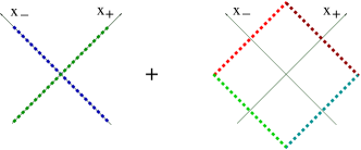
Figure 9: Wilson-line structure of the effective action .

In should be emphasized that Eq. (67) is only a model - the genuine effective action for the $2+1$ high-energy theory of Wilson lines must include all the contributions $\sim[U,V]^{n}$ (as we mentioned above, an example of a $[U,V]^{3}$ term which is missing in Eq. (22) is presented in Fig. 8). However, this model is correct in the case of weak projectile fields and strong target fields, and vice versa. In terms of Feynman diagrams, the effective action (67) includes both “up” and “down” fan ladders and the pomeron loops, see Fig. 10. In the dipole language, it describes both multiplication and recombination of dipoles (see the discussion in murecent ; larecent ).

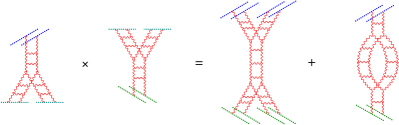
Figure 10: Typical Feynman diagrams included in the effective action.

In conclusion I would like to emphasize that the effective action (67) summarizes all present knowledge about the high-energy evolution of Wilson lines in a way symmetric with respect to projectile and target and hence it may serve as a starting point for future analysis of high-energy scattering in QCD.

Appendix A Classical fields in the first order in $[U,V]$

Following Ref. prd04 , we take the zero-order approximation in the form of the sum of the two shock waves (23)

$$\bar{A}_{i}^{(0)}=U_{i}\theta(-x_{\ast})+V_{i}\theta(-x_{\bullet}),~{}~{}~{}\bar{A}_{\bullet}^{(0)}=\bar{A}_{\ast}^{(0)}=0$$ (82)

We will expand the “deviation” of the full QCD solution from the QED-type ansatz (82) in powers of commutators $[U,V]$. To carry this out, we shift $A\rightarrow A+\bar{A}_{i}^{(0)}$ in the functional integral (22) and obtain

$$\int\!DA~{}\exp\Big{\{}i\!\int\!d^{4}z({1\over 2}A^{\mu}\bar{D}_{\mu\nu}A^{\nu}+gT^{\mu}A_{\mu})\Big{\}}.$$ (83)

Here $D_{\mu\nu}=D^{2}(\bar{A})g_{\mu\nu}-2i\bar{F}_{\mu\nu}$ is the inverse propagator in the background-Feynman gauge and $T_{\mu}$ is the linear term for the trial configuration (82). Since the only non-zero component of the field strength for the ansatz (82) is

$$\bar{F}^{(0)}_{ik} = -i[U_{1i},V_{1k}]\theta(F)-i[U_{1i},V_{2k}]\theta(R)$$

$$- i[U_{2i},V_{1k}]\theta(L)-i[U_{2i},V_{2k}]\theta(B)-(i\leftrightarrow k)$$

the linear term $T_{\mu}=\bar{D}^{\rho}\bar{F}^{(0)}_{\rho\mu}$ is

$$T_{\ast}~{}=~{}T_{\bullet}~{}=~{}0,$$ (85)

$$T^{i}~{}=~{}(i\partial_{k}+g[U_{1k}+V_{1k},)([U_{1}^{i},V_{1}^{k}]-i\leftrightarrow k)\theta(F)$$

$$+~{}(i\partial_{k}+g[U_{1k}+V_{2k},)([U_{1}^{i},V_{2}^{k}]-i\leftrightarrow k)\theta(R)$$

$$+~{}(i\partial_{k}+g[U_{2k}+V_{2k},)([U_{2}^{i},V_{1}^{k}]-i\leftrightarrow k)\theta(L)$$

$$+~{}(i\partial_{k}+g[U_{2k}+V_{2k},)([U_{2}^{i},V_{2}^{k}]-i\leftrightarrow k)\theta(B)$$

where $\theta(F)\equiv\theta(z_{\ast})\theta(z_{\bullet})$, $\theta(R)\equiv\theta(z_{\ast})\theta(-z_{\bullet})$, $\theta(L)\equiv\theta(-z_{\ast})\theta(z_{\bullet})$, and $\theta(B)\equiv\theta(-z_{\ast})\theta(-z_{\bullet})$

Expanding in powers of $T$ in the functional integral (83) one gets the set of Feynman diagrams in the external fields (23) with the sources (85). The parameter of the expansion is $g^{2}[U_{i},V_{j}]$ ($\sim[U,V]$, see Eq. (5)).

The general formula for the classical solution in the first order in $[U,V]$ has the form

$$\bar{A}^{(1)a}_{\mu}(x) = ig\!\int\!d^{4}z\langle A^{a}_{\mu}(x)A^{b\nu}(z)\rangle_{\bar{A}}T^{b}_{\nu}(z)$$ (86)

The Green functions in the background of the Eq. (23) field can be approximated by cluster expansion

$$\langle A_{\mu}(x)A^{\nu}(z)\rangle_{\bar{A}}$$

$$=~{}\langle A_{\mu}(x)A^{\nu}(z)\rangle_{U}+\langle A_{\mu}(x)A^{\nu}(z)\rangle_{V}$$

$$-~{}\langle A_{\mu}(x)A^{\nu}(z)\rangle_{0}+O([U,V])$$ (87)

where $\langle A_{\mu}(x)A^{\nu}(z)\rangle_{0}$ is the perturbative propagator and

$$\langle A^{a}_{\mu}(x)A^{b}_{\nu}(y)\rangle_{U}\stackrel{{\scriptstyle x_{\ast}>0,y_{\ast}<0}}{{~{}=~{}}}\!\int\!dz\delta({2\over s}z_{\ast})~{}\Big{\{}U^{\dagger}_{1x}(x|{1\over p^{2}+i\epsilon}|z)$$

$$\times~{}\Big{(}2\alpha g_{\mu\nu}U_{1}U_{2}^{\dagger}+{4i\over s}(p_{2\nu}\partial_{\mu}(U_{1}U_{2}^{\dagger})_{z}+\mu\leftrightarrow\nu)$$

$$-~{}{4p_{2\mu}p_{2\nu}\over\alpha s^{2}}\partial_{\perp}^{2}(U_{1}U_{2}^{\dagger})_{z}\Big{)}(z|{1\over p^{2}+i\epsilon}|y)U_{2y}\Big{)}^{ab}$$ (88)

is the propagator in the background of the shock wave $U$ (the propagator in the $V$ background is obtained by the replacement $U\leftrightarrow V$, $p_{2}\leftrightarrow p_{1}$.

Substituting Eq. (88) and (85) into the above equation, one obtains (the details of the calculations can be found in Ref. prd04 and here we present only the the final set of gauge fields):

$$A^{\mu} = \theta(F)\Big{\{}{\cal W}^{\mu\perp}_{F}(x_{\perp})-gt^{a}(W_{F}^{\dagger}{1\over\partial^{2}-i\epsilon}W_{F})^{ab}L_{F}^{\mu b}(x)\Big{\}}$$ (89)

$$+ (F\leftrightarrow L)+(F\leftrightarrow R)+(F\leftrightarrow B)$$

where $L_{F}^{i}~{}=~{}L_{L}^{i}~{}=~{}L_{R}^{i}~{}=~{}L_{B}^{i}~{}=~{}2E^{i}$ and

$$L_{F\ast} = 2[V_{1i}-V_{2i},{1\over\beta+i\epsilon}E_{R}^{i}-{1\over\beta-i\epsilon}E_{B}^{i}]$$

$$L_{F\bullet} = 2[U_{1i}-U_{2i},{1\over\alpha+i\epsilon}E_{L}^{i}-{1\over\alpha-i\epsilon}E_{B}^{i}]$$

$$L_{L\ast} = 2[V_{1i}-V_{2i},{1\over\beta+i\epsilon}E_{R}^{i}-{1\over\beta-i\epsilon}E_{B}^{i}]$$

$$L_{L\bullet} = 2[U_{1i}-U_{2i},{1\over\alpha+i\epsilon}E_{F}^{i}-{1\over\alpha-i\epsilon}E_{R}^{i}]$$

$$L_{R\ast} = 2[V_{1i}-V_{2i},{1\over\beta+i\epsilon}E_{F}^{i}-{1\over\beta-i\epsilon}E_{L}^{i}]$$

$$L_{R\bullet} = 2[U_{1i}-U_{2i},{1\over\alpha+i\epsilon}E_{L}^{i}-{1\over\alpha-i\epsilon}E_{B}^{i}]$$

$$L_{B\ast} = 2[V_{1i}-V_{2i},{1\over\beta+i\epsilon}E_{F}^{i}-{1\over\beta-i\epsilon}E_{L}^{i}]$$

$$L_{B\bullet} = [U_{1i}-U_{2i},{1\over\alpha+i\epsilon}E_{F}^{i}-{1\over\alpha-i\epsilon}E_{R}^{i}]$$ (90)

where ${2/s\over\alpha\pm i\epsilon}{\cal O}(x)\equiv i\int_{0}^{\pm\infty}du{\cal O}(x+up_{2})$ and ${2/s\over\beta\pm i\epsilon}{\cal O}(x)\equiv i\int_{0}^{\pm\infty}du{\cal O}(x+up_{1})$. It is easy to check the background-Feynman gauge condition $(i\partial_{\mu}+g[{\cal W}_{F}^{\mu},)L_{F\mu}=0$ (and similarly for three other quadrants of the space).

The transverse part $E_{i}$ agrees with the results of Sec. while the longitudinal part (90) does not literally agree with (32) (see the footnote after that equation). It should be emphasized that, unlike the calculations with trial configuration (25), the Feynman diagrams in the background of the ansatz (82) are free from uncertainties like $\theta(0)$.

Let us rederive now the effective action (39) starting from the ansatz (82) and the fields (89). Since the only non-zero component of the field strength for the ansatz (82) is transverse (see Eq. (A), we have

$$S_{\rm eff}~{}=~{}-{1\over 4}\!\int\!d^{4}z\bar{F}^{(0)a}_{ik}\bar{F}^{(0)a,ik}$$

$$+~{}{i\over 2}\!\int\!d^{4}zd^{4}z^{\prime}T^{a}_{i}(z)T^{b}_{j}(z^{\prime})\langle A^{ai}(z)A^{bj}(z^{\prime})\rangle$$

$$=~{}-{1\over 4}\!\int\!d^{4}z\Big{(}\bar{F}^{(0)a}_{ik}\bar{F}^{(0)a,ik}$$

$$+~{}i\!\int\!d^{4}z^{\prime}\bar{F}^{(0)a}_{ik}(z)\langle(\bar{D}^{i}A^{ak}(z)-i\leftrightarrow k)A^{bj}(z^{\prime})\rangle T^{b}_{j}(z^{\prime})\Big{\}}$$

$$=~{}-{1\over 4}\!\int\!d^{4}z\bar{F}^{(0)a}_{ik}\bar{F}^{(1)a,ik}$$ (91)

where $\bar{F}^{(1)a,ik}$ is a field strength in the first order in $[U,V]$. Using the fields (89) we obtain

$$F^{(1)a}_{ik}(z) = -2g\theta(F)(z|W_{F}^{\dagger}{\partial_{i}\over\partial^{2}-i\epsilon}W_{F}|^{ab}0,E_{k}^{b})$$

$$+ (F\leftrightarrow L)+(F\leftrightarrow R)+(F\leftrightarrow B)-(i\leftrightarrow k)$$

(where $|0,E_{i})\equiv\int d^{2}z^{\prime}_{\perp}|0,z^{\prime}_{\perp})E_{i}(z^{\prime}_{\perp})$) and therefore

$$S_{\rm eff}~{}$$ (93)

$$=~{}-ig^{2}\!\!\int\!d^{4}z\Big{\{}\theta(F)([U_{1}^{i},V_{1}^{k}]-i\leftrightarrow k)^{a}(W_{F}^{\dagger}{\partial_{i}\over\partial^{2}}W_{F})^{ab}E_{k}^{b}$$

$$\hskip 28.45274pt+~{}\theta(R)([U_{1}^{i},V_{2}^{k}]-i\leftrightarrow k)^{a}(W_{R}^{\dagger}{\partial_{i}\over\partial^{2}}W_{R})^{ab}E_{k}^{b}$$

$$\hskip 28.45274pt+~{}\theta(L)([U_{2}^{i},V_{1}^{k}]-i\leftrightarrow k)^{a}(W_{L}^{\dagger}{\partial_{i}\over\partial^{2}}W_{L})^{ab}E_{k}^{b}$$

$$\hskip 28.45274pt+~{}\theta(L)([U_{2}^{i},V_{2}^{k}]-i\leftrightarrow k)^{a}(W_{B}^{\dagger}{\partial_{i}\over\partial^{2}}W_{B})^{ab}E_{k}^{b}\Big{\}}$$

A typical integral in the above equation has the form

$$\int\!d^{4}zd^{2}z^{\prime}_{\perp}~{}\theta(z_{\ast})\theta(z_{\bullet})f(z_{\perp})(z|{p_{i}\over p^{2}+i\epsilon}|0,z^{\prime}_{\perp})g(z^{\prime}_{\perp})$$

$$={i\over 2\pi}\!\int_{0}^{\infty}\!{d\alpha\over\alpha}\!\int\!d^{2}z_{\perp}d^{2}z^{\prime}_{\perp}f(z_{\perp})(z_{\perp}|{p_{i}\over p_{\perp}^{2}}|z^{\prime}_{\perp})g(z^{\prime}_{\perp})$$ (94)

In the LLA, the integral $\!\int_{0}^{\infty}\!{d\alpha\over\alpha}$ is replaced by ${1\over 2}\Delta\eta$. More accurately, one should remember that the slopes of Wilson lines are $e_{1}=p_{1}+e^{-\eta_{1}}p_{2}$ and $e_{2}=p_{2}+e^{\eta_{2}}p_{1}$ as shown in Eq. (14). In this case, $\theta(z_{\ast})\theta(z_{\bullet})$ in the integrand of Eq. (94) will be replaced by $\theta(z_{\ast}+e^{\eta_{2}}z_{\bullet})\theta(z_{\bullet}+e^{-\eta_{1}}z_{\ast})$ so one obtains

$$\int\!d^{4}zd^{2}z^{\prime}_{\perp}~{}\theta(z_{\ast})\theta(z_{\bullet})f(z_{\perp})(z|{p_{i}\over p^{2}+i\epsilon}|0,z^{\prime}_{\perp})g(z^{\prime}_{\perp})$$

$$=~{}-\!\int\!d^{2}z_{\perp}d^{2}z^{\prime}_{\perp}f(z_{\perp})g(z^{\prime}_{\perp})\!\int\!{d\alpha d\beta d^{2}p_{\perp}\over 16\pi^{4}}~{}e^{i(p,z-z^{\prime})_{\perp}}$$

$$\times~{}{p_{i}\over\alpha\beta s-p_{\perp}^{2}+i\epsilon}~{}{1\over(\alpha+e^{\eta_{2}}\beta-i\epsilon)(\beta+e^{-\eta_{1}}\alpha-i\epsilon)}$$

$$=~{}-i\!\int\!d^{2}z_{\perp}d^{2}z^{\prime}_{\perp}f(z_{\perp})g(z^{\prime}_{\perp})\!\int_{0}^{\infty}\!{d\alpha\over\alpha}{d^{2}p_{\perp}\over 8\pi^{3}}~{}e^{i(p,z-z^{\prime})_{\perp}}$$

$$\times~{}\Big{(}{p_{i}\over e^{-\eta_{1}}\alpha^{2}s+p_{\perp}^{2}}-{p_{i}\over e^{-\eta_{2}}\alpha^{2}s+p_{\perp}^{2}}\Big{)}$$

$$=~{}-{i\over 4\pi}\Delta\eta\!\int\!d^{2}z_{\perp}d^{2}z^{\prime}_{\perp}f(z_{\perp})(z_{\perp}|{p_{i}\over p_{\perp}^{2}}|z^{\prime}_{\perp})g(z^{\prime}_{\perp})$$ (95)

where $\Delta\eta=\eta_{1}-\eta_{2}$. Performing the integrations over $z_{\ast},z_{\bullet}$ in Eq. (93) we get

$$S_{\rm eff}$$ (96)

$$=~{}-\alpha_{s}\Delta\eta\!\int\!d^{2}z_{\perp}\Big{\{}([U_{1}^{i},V_{1}^{k}]-i\leftrightarrow k)^{a}(W_{F}^{\dagger}{\partial_{i}\over\partial_{\perp}^{2}}W_{F})^{ab}$$

$$\hskip 28.45274pt-~{}([U_{1}^{i},V_{2}^{k}]-i\leftrightarrow k)^{a}(W_{R}^{\dagger}{\partial_{i}\over\partial_{\perp}^{2}}W_{R})^{ab}$$

$$\hskip 28.45274pt-~{}([U_{2}^{i},V_{1}^{k}]-i\leftrightarrow k)^{a}(W_{L}^{\dagger}{\partial_{i}\over\partial_{\perp}^{2}}W_{L})^{ab}$$

$$\hskip 28.45274pt+~{}([U_{2}^{i},V_{2}^{k}]-i\leftrightarrow k)^{a}(W_{B}^{\dagger}{\partial_{i}\over\partial_{\perp}^{2}}W_{B})^{ab}\Big{\}}E_{k}^{b}$$

$$=~{}-i\alpha_{s}\Delta\eta\!\int\!d^{2}z_{\perp}~{}E_{i}^{a}E^{ai}$$

which coincides with Eq. (39).

Finally, let us demonstrate that the “diamond” trace of four (non-differentiated) Wilson lines is trivial (this is related to the fact that the field strength $F_{+-}$ vanishes in the leading order, see Eqs. (89) and (90)). To regularize the corresponding expressions, we consider the “original” tilted Wilson loop shown in Fig. 11 for the finite size $L$.

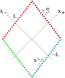
Figure 11: Trace of four Wilson lines.

We need to prove that

$$\lim_{L\rightarrow\infty}{\rm tr}\{[-Le_{1}+Le_{2}+x_{\perp},Le_{1}+Le_{2}+x_{\perp}]$$ (97)

$$\hskip 8.53581pt\times~{}[Le_{2}+Le_{1}+x_{\perp},-Le_{2}+Le_{1}+x_{\perp}]$$

$$\hskip 8.53581pt\times~{}[Le_{1}-Le_{2}+x_{\perp},-Le_{1}-Le_{2}+x_{\perp}]$$

$$\hskip 8.53581pt\times~{}[-Le_{2}-Le_{2}+x_{\perp},Le_{2}-Le_{2}+x_{\perp}]\}~{}=~{}1$$

in the leading nontrivial order in $[U,V]$ .

Consider the case ${\cal U}_{i}\ll 1$, ${\cal V}_{i}\sim 1$ (the opposite case ${\cal V}_{i}\ll 1$, ${\cal U}_{i}\sim 1$ is similar). It is easy to see from Eq. (90) that $[Le_{2}\pm Le_{1}+x_{\perp},-Le_{2}\pm Le_{1}+x_{\perp}]\sim[U,V]^{2}$ so we are left with

$$\lim_{L\rightarrow\infty}{\rm tr}\{[-Le_{1}+Le_{2}+x_{\perp},Le_{1}+Le_{2}+x_{\perp}]$$

$$\times~{}[Le_{1}-Le_{2}+x_{\perp},-Le_{1}-Le_{2}+x_{\perp}]\}$$ (98)

At this point, we can take the limit $L\rightarrow\infty$ in the $e_{1}$ direction. We obtain:

$$[x_{\perp}+Le_{2},x_{\perp}+Le_{2}+\infty e_{1}]$$ (99)

$$\hskip 36.98857pt\times~{}[x_{\perp}-Le_{2}+\infty e_{1},x_{\perp}-Le_{2}]-1$$

$$=~{}{i\over\pi^{2}}\!\int\!d\alpha d\beta~{}{\sin\alpha L\over(\alpha+e^{\eta_{2}}\beta-i\epsilon)(\beta+e^{-\eta_{1}}\alpha-i\epsilon)}$$

$$\times~{}(x_{\perp}|U_{1}^{\dagger}{1\over\alpha\beta s-p_{\perp}^{2}+i\epsilon}U_{1}|^{ab}|[U_{1i}-U_{2i},E_{L}^{i}-E_{2}^{i}]^{b})$$

$$=-{2\over\pi}\!\int_{0}^{\infty}\!d\alpha~{}{\sin\alpha L\over\alpha}(x_{\perp}|U_{1}^{\dagger}\Big{(}{1\over e^{-\eta_{1}}\alpha^{2}s+p_{\perp}^{2}}$$

$$\hskip 8.53581pt-~{}{1\over e^{-\eta_{2}}\alpha^{2}s+p_{\perp}^{2}}\Big{)}U_{1}|^{ab}|[U_{1i}-U_{2i},E_{L}^{i}-E_{2}^{i}]^{b})$$

We see now that in the limit $L\rightarrow\infty$ the r.h.s. of Eq. (100) vanishes so the l.h.s. is at best $\sim[U,V]^{2}$ . Similarly,

$$\lim_{L\rightarrow\infty}[x_{\perp}+Le_{2},x_{\perp}+Le_{2}-\infty e_{1}]$$ (100)

$$\hskip 36.98857pt\times~{}[x_{\perp}-Le_{2}-\infty e_{1},x_{\perp}-Le_{2}]~{}=~{}1$$

and therefore the trace (98), which is product of l.h.s. of Eq. (99) and Eq. (100), is equal to 1 in the leading order.

References

References

- (1) I. Balitsky, “High-Energy QCD and Wilson Lines”, In *Shifman, M. (ed.): At the frontier of particle physics, vol. 2*, p. 1237-1342 (World Scientific, Singapore,2001) [hep-ph/0101042]
- (2) L.V. Gribov, E.M. Levin, and M.G. Ryskin, Phys. Rept. 100, 1 (1983).
- (3) A.H. Mueller and J.W. Qiu Nucl. Phys. B268, 427 (1986).
- (4) A.H. Mueller, Nucl. Phys. B335, 115 (1990).
- (5) A.H. Mueller, Nucl. Phys. B558, 285 (1999);
- (6) M.A. Braun, Eur.Phys.J.C16, 337 (2000); Phys. Lett. B 483, 115 (2000).
- (7) E. Iancu, K. Itakura, and L. McLerran, Nucl. Phys. A708, 327 (2002).
- (8) M. Lublinsky, Eur. Phys. J.C21, 513 (2001); K. Colec-Biernart, L. Motyka, A.M. Stasto, Phys. Rev. D65, 074037 (2002); N. Armesto and M.A. Braun, Eur.Phys.J.C20, 517 (2001); J.L. Albacete, A. Kovner, C.A. Salgado, and U.A. Wiedemann, Phys. Rev. Lett. 92, 082001 (2003).
- (9) L. McLerran and R. Venugopalan, Phys. Rev. D49, 2233 (1994); Phys. Rev. D49, 3352 (1994).
- (10) A. Kovner, L. McLerran and H. Weigert, Phys. Rev. D52, 3809 (1995); Phys. Rev. D52, 6231 (1995).
- (11) I. Balitsky, Phys. Rev. D60, 014020 (1999).
- (12) A. Krasnitz and R. Venugopalan, Nucl. Phys. B557, 237 (1999); Phys. Rev. Lett. 84, 4309 (2000).
- (13) Yu. V. Kovchegov and A.H. Mueller, Nucl. Phys. B529, 451 (1998).
- (14) B.Z Kopeliovich, A. Schafer, and A.V. Tarasov, Phys. Rev. D62, 054022 (2000); B.Z Kopeliovich Phys. Rev. C68, 044906 (2003).
- (15) A. Kovner and U. Wiedemann, Phys. Rev. D64, 114002 (2001);
- (16) I. Balitsky, Phys. Rev. D70, 114030 (2004).
- (17) Y. Hatta, E. Iancu, L. McLerran, A. Stasto , and D.N. Triantafyllopoulos “Effective Hamiltonian for QCD evolution at high energy”, [hep-ph/0504182].
- (18) Y. Hatta, E. Iancu, L. McLerran, A. Stasto , and D.N. Triantafyllopoulos, “Color Dipoles from Bremsstrahlung in QCD Evolution at High Energy”, [hep-ph/0505235].
- (19) A. Kovner and M. Lublinsky, Phys.Rev.D71, 085004(2005); Phys.Rev.Lett.9, 181603(2005); JHEP, 0503:001(2005)
- (20) A.H. Mueller, A.I. Shoshi, and S.M.H. Wong, Nucl.Phys.B715, 440(2005).
- (21) C. Marquet, A.H. Mueller, A.I. Shoshi, and S.M.H. Wong, “ On the Projectile-target Duality of the Color Glass Condensate in the Dipole Picture”, [hep-ph/0402256].
- (22) E. Levin , “High-Energy Amplitude in the Dipole Approach with Pomeron Loops: Asymptotic Solution”, [hep-ph/0502243]; E. Levin and M. Lublinsky, “Towards a Symmetric Approach to High-Energy Evolution: Generating Functional with Pomeron Loops”, [hep-ph/0501173]
- (23) I. Balitsky, Phys. Rev. Lett. 81, 2024 (1998).
- (24) A. Babansky and I. Balitsky, Phys. Rev. D67, 054026 (2003).
- (25) E-M. Ilgenfritz, Yu.P. Ivanov, and H.J. Pirner Phys. Rev. D62, 054006 (2000); H. J. Pirner and F. Yuan, Phys. Rev. D66, 034020 (2002).
- (26) I. Balitsky, Nucl. Phys. B463, 99 (1996).
- (27) Yu.V. Kovchegov, Phys. Rev. D60, 034008 (1999); Phys. Rev. D61, 074018 (2000).
- (28) L.N. Lipatov, Nucl.Phys.B452, 369(1995), Phys.Rept.286, 131(1997).
- (29) I. Balitsky, Phys. Lett. B 518, 235 (2001).
- (30) I. Balitsky, “Operator expansion for diffractive high-energy scattering”, [hep-ph/9706411].
- (31) J. Jalilian-Marian, A. Kovner, A. Leonidov and H. Weigert, Nucl. Phys.B504, 415 (1997), Phys. Rev.D59, 014014 (1999), J. Jalilian-Marian, A. Kovner and H. Weigert, Phys. Rev. D59, 014015 (1999), A. Kovner, J. G. Milhano and H. Weigert, Phys. Rev. D62, 114005 (2000); E. Iancu, A. Leonidov and L. McLerran, Nucl. Phys.A692, 583 (2001), Phys. Lett.B510, 133 (2001), E. Ferreiro, E. Iancu, A. Leonidov and L. McLerran, Nucl. Phys.A703, 489 (2002).