2005 International Linear Collider Workshop - Stanford, U.S.A.
CERN-PH-TH/2005-120
 
Resolving ambiguities in mass determinations at future colliders

Abstract

The measurements of kinematical endpoints, in cascade decays of supersymmetric particles, in principle allow for a determination of the masses of the unstable particles. However, in this procedure ambiguities often arise. We here illustrate how such ambiguities arise. They can be resolved by a precise determination of the LSP mass, provided by the Linear Collider.

I INTRODUCTION

If R-parity conserving supersymmetry exists below the TeV-scale, new particles will be produced and decay in cascades at the LHC. The lightest supersymmetric particle will escape the detectors, thereby complicating the full reconstruction of the decay chains. However, the masses of the particles in a cascade like

$$\tilde{q}_{L}\to{\tilde{\chi}^{0}_{2}}q\to{\tilde{l}_{R}}^{\mp}l_{\rm n}^{\pm}q\to{\tilde{\chi}^{0}_{1}}l_{\rm f}^{\mp}l_{\rm n}^{\pm}q$$ (1)

can be determined from endpoints of kinematical distributions Baer:1995va ; Allanach:2000kt ; Gjelsten:2004ki . Here, $\tilde{q}_{L}$ denotes a (left-handed) squark, ${\tilde{l}_{R}}$ a (right-handed) slepton, whereas ${\tilde{\chi}^{0}_{2}}$ and ${\tilde{\chi}^{0}_{1}}$ denote the lightest neutralinos, the latter being stable. The observed leptons and quark (jet) are denoted $l_{\rm n}$, $l_{\rm f}$ and $q$, where the subscripts “n” and “f” denote “near” and “far”.

Attention is focused on the mSUGRA benchmark point SPS 1a (line) Allanach:2002nj

$$m_{0}=-A_{0}=0.4\,m_{1/2},\quad\tan\beta=10,\quad\mu>0,$$ (2)

and in particular two points on the line, SPS 1a ($\alpha$) with $m_{0}=100~{}\text{GeV}$ and $m_{1/2}=250~{}\text{GeV}$, and SPS 1a ($\beta$) with $m_{0}=160~{}\text{GeV}$ and $m_{1/2}=400~{}\text{GeV}$. The resulting low-energy masses entering in the cascade (1) are given in Table 1 Gjelsten:2004ki .

Table 1: SPS 1a masses

	$m_{{\tilde{q}_{L}}}$ [GeV]	$m_{{\tilde{\chi}^{0}_{2}}}$ [GeV]	$m_{{\tilde{l}_{R}}}$ [GeV]	$m_{{\tilde{\chi}^{0}_{1}}}$ [GeV]
($\alpha$)	537.2	176.8	143.0	96.1
($\beta$)	826.3	299.1	221.9	161.0

Invariant masses involving various subsets of the observed particles, namely the quark, $q$ and the two leptons, $l_{\rm n}$ and $l_{\rm f}$, can be reconstructed. Since the “near” and “far” leptons can not be distinguished, one must instead, on an event-by-event basis, define a “high” and “low” distribution, such that

$$m_{ql({\rm low})}=\min(m_{ql_{\rm n}},m_{ql_{\rm f}}),\quad m_{ql({\rm high})}={\rm max}(m_{ql_{\rm n}},m_{ql_{\rm f}}).$$ (3)

From a knowledge of kinematical endpoints, in particular those of the $m_{qll}$, $m_{ql({\rm low})}$, $m_{ql({\rm high})}$ and $m_{ll}$ distributions, the masses of the unstable particles can be reconstructed. Indeed, the endpoints of these distributions can be expressed explicitly in terms of $m_{{\tilde{q}_{L}}}$, $m_{{\tilde{\chi}^{0}_{2}}}$, $m_{{\tilde{l}_{R}}}$ and $m_{{\tilde{\chi}^{0}_{1}}}$ Allanach:2000kt ; Gjelsten:2004ki . Additional information can be obtained from threshold determinations Allanach:2000kt , and the method can be extended to the case of a gluino at the head of the chain Gjelsten:2005aw .

II COMPOSITE FORMULAS

Many of the problems which arise in this method are related to the fact that the kinematical endpoints are composite functions of the unknown masses. Indeed, the functional form for $m^{\rm max}_{qll}$, $m^{\rm max}_{ql({\rm low})}$ and $m^{\rm max}_{ql({\rm high})}$ depend on the relative mass ratios. For $m^{\rm max}_{ql({\rm low})}$ and $m^{\rm max}_{ql({\rm high})}$, they are given by Allanach:2000kt ; Gjelsten:2004ki :

$$\big{(}m^{\rm max}_{ql({\rm low})},m^{\rm max}_{ql({\rm high})}\big{)}=\left\{\begin{array}[]{llcc}\big{(}m^{\rm max}_{ql_{\rm n}},m^{\rm max}_{ql_{\rm f}}\big{)}&\quad{\rm for}&2{m_{\tilde{l}_{R}}^{2}}>{m_{\tilde{\chi}^{0}_{1}}^{2}}+{m_{\tilde{\chi}^{0}_{2}}^{2}}>2m_{{\tilde{\chi}^{0}_{1}}}m_{{\tilde{\chi}^{0}_{2}}}&\quad{\it(1)}\\[11.38109pt] \big{(}m^{\rm max}_{ql({\rm eq})},m^{\rm max}_{ql_{\rm f}}\big{)}&\quad{\rm for}&{m_{\tilde{\chi}^{0}_{1}}^{2}}+{m_{\tilde{\chi}^{0}_{2}}^{2}}>2{m_{\tilde{l}_{R}}^{2}}>2m_{{\tilde{\chi}^{0}_{1}}}m_{{\tilde{\chi}^{0}_{2}}}&\quad{\it(2)}\\[11.38109pt] \big{(}m^{\rm max}_{ql({\rm eq})},m^{\rm max}_{ql_{\rm n}}\big{)}&\quad{\rm for}&{m_{\tilde{\chi}^{0}_{1}}^{2}}+{m_{\tilde{\chi}^{0}_{2}}^{2}}>2m_{{\tilde{\chi}^{0}_{1}}}m_{{\tilde{\chi}^{0}_{2}}}>2{m_{\tilde{l}_{R}}^{2}}&\quad{\it(3)}\end{array}\right\}$$ (4)

with

$$\big{(}m^{\rm max}_{ql_{\rm n}}\big{)}^{2} = \big{(}{m_{\tilde{q}_{L}}^{2}}-{m_{\tilde{\chi}^{0}_{2}}^{2}}\big{)}\big{(}{m_{\tilde{\chi}^{0}_{2}}^{2}}-{m_{\tilde{l}_{R}}^{2}}\big{)}/{m_{\tilde{\chi}^{0}_{2}}^{2}}$$ (5)

$$\left(m^{\rm max}_{ql_{\rm f}}\right)^{2} = \big{(}{m_{\tilde{q}_{L}}^{2}}-{m_{\tilde{\chi}^{0}_{2}}^{2}}\big{)}\big{(}{m_{\tilde{l}_{R}}^{2}}-{m_{\tilde{\chi}^{0}_{1}}^{2}}\big{)}/{m_{\tilde{l}_{R}}^{2}}$$ (6)

$$\big{(}m^{\rm max}_{ql({\rm eq})}\big{)}^{2} = \big{(}{m_{\tilde{q}_{L}}^{2}}-{m_{\tilde{\chi}^{0}_{2}}^{2}}\big{)}\big{(}{m_{\tilde{l}_{R}}^{2}}-{m_{\tilde{\chi}^{0}_{1}}^{2}}\big{)}/\big{(}2{m_{\tilde{l}_{R}}^{2}}-{m_{\tilde{\chi}^{0}_{1}}^{2}}\big{)}$$ (7)

In this report we will focus on $m^{\rm max}_{ql({\rm low})}$ and $m^{\rm max}_{ql({\rm high})}$ as functions of $m_{{\tilde{\chi}^{0}_{1}}}$, since the behaviour of these two endpoints is most important for the mSUGRA points studied. In the case of $m^{\rm max}_{ql({\rm low})}$, the functional form changes when $m_{{\tilde{\chi}^{0}_{1}}}$ crosses $\sqrt{2m_{{\tilde{l}_{R}}}^{2}-m_{{\tilde{\chi}^{0}_{2}}}^{2}}$, whereas for $m^{\rm max}_{ql({\rm high})}$ it changes when $m_{{\tilde{\chi}^{0}_{1}}}$ crosses $m_{{\tilde{l}_{R}}}^{2}/m_{{\tilde{\chi}^{0}_{2}}}$. The three cases given in eq. (4) are in Gjelsten:2004ki referred to as regions (1,1), (1,2) and (1,3), where the first index (“1”) refers to the expression for $m^{\rm max}_{qll}$, which remains unchanged. The corresponding critical mass values are given in Table 2 for $m_{{\tilde{\chi}^{0}_{1}}}$, keeping the other masses at their nominal SPS 1a values.

Table 2: Region borders for $m_{{\tilde{\chi}^{0}_{1}}}$ [GeV]

	SPS 1a nominal	Region (1,1) vs. (1,2)	Region (1,2) vs. (1,3)
($\alpha$)	96.1	98.2	115.7
($\beta$)	161.0	95.0	164.6

Thus, the functional forms for $m^{\rm max}_{ql({\rm low})}$ and $m^{\rm max}_{ql({\rm high})}$ change very close to the nominal values of $m_{{\tilde{\chi}^{0}_{1}}}$ for SPS 1a ($\alpha$) and ($\beta$), respectively, as is illustrated in Fig. 1. These points are close to the transitions from region (1,1) to (1,2), and from region (1,2) to (1,3), respectively.

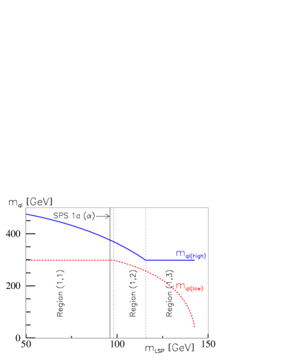
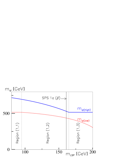
Figure 1: The invariants $m^{\rm max}_{ql({\rm low})}$ and $m^{\rm max}_{ql({\rm high})}$ are composite functions of $m_{{\tilde{\chi}^{0}_{1}}}$ (denoted $m_{\rm LSP}$). Other masses are held fixed at respectively the SPS 1a ($\alpha$) (left panel) and SPS 1a ($\beta$) (right panel) values.

III AMBIGUITIES

Ambiguities in the masses extracted from endpoint measurements are principally caused by the analytic form of the endpoint expressions, as seen above. In particular, they frequently lead to multiple solutions in mass-space for a particular set of endpoint values, even when experimental uncertainties are neglected. Furthermore, inclusion of extra overconstraining measurements moves solutions about in mass-space and can destroy or create new ones, adding to the complexity.

III.1 Multiple solutions

In this subsection we restrict the discussion to the case in which the number of available (linearly independent) endpoints is equal to the number of masses involved. In particular we have in mind the standard case where $m^{\rm max}_{ll}$, $m^{\rm max}_{ql({\rm low})}$, $m^{\rm max}_{ql({\rm high})}$ and $m^{\rm max}_{qll}$ are measured. In this situation analytic expressions for the masses in terms of the endpoints can be obtained Gjelsten:2004ki , which in a numerical fit would correspond to solutions with $\chi^{2}=0$. While the endpoints are obviously single-valued functions of the masses, due to the composite (and quadratic) form of the endpoint expressions the inverse is in general not true. A specific set of endpoint values can often be produced by several sets of masses. This ambiguity is illustrated in Fig. 2, where multiple solutions in the $\chi^{2}$ fit become evident. In this fit, the four kinematical endpoints $m^{\rm max}_{ll}$, $m^{\rm max}_{ql({\rm low})}$, $m^{\rm max}_{ql({\rm high})}$ and $m^{\rm max}_{qll}$ are taken at their nominal values, and for each value of $m_{{\tilde{\chi}^{0}_{1}}}$ in the figure, the other three masses are allowed to vary. The left panel is devoted to SPS 1a ($\alpha$), whereas the right panel is devoted to SPS 1a ($\beta$). Three mass regions are realised; (1,1), (1,2) and (1,3), as well as the border between (1,2) and (1,3), denoted “B”. Vertical lines separate the regions in the $m_{\rm LSP}$ scans.

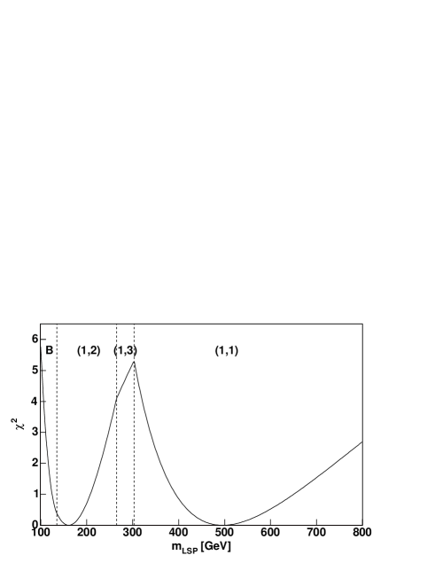
Figure 2: $\chi^{2}$ vs. $m_{{\tilde{\chi}^{0}_{1}}}$, allowing the other masses to vary. Left: SPS 1a ($\alpha$), Right: SPS 1a ($\beta$).

We clearly see that for four endpoint measurements, multiple mass sets provide the same endpoints and create an ambiguity at both the investigated mSUGRA points. For each of the two plots the non-smooth parts of the curve correspond to discontinuities in the mass-space trajectory defined by the (ordered) collection of best-fit masses found from the scan. At these points two identically good minima exist and a jump is made from one to the other. While the scanned mass $m_{{\tilde{\chi}^{0}_{1}}}$ obviously changes smoothly, the other masses have discontinuities at these points. For the two investigated mSUGRA scenarios and in particular SPS 1a ${(\beta)}$, $m_{{\tilde{l}_{R}}}$ and $m_{{\tilde{q}_{L}}}$, more so than $m_{{\tilde{\chi}^{0}_{2}}}$, change considerably at these discontinuities, the first by roughly 5%.

III.2 Overconstrained systems

When an extra endpoint measurement, such as the $qll$ “threshold”, is introduced, the system becomes overconstrained, with five measurements determining only four masses. One might expect this to alleviate the ambiguity from multiple solutions seen in the previous section, since the extra endpoint should ‘pick out’ one of the solutions. However, this is not always the case: the uncertainty of endpoint measurements and the introduction of an overconstraining measurement will move the solutions around in mass-space, possibly creating new solutions, or destroying old ones. This may then cause a further ambiguity, additional to that seen in III.1, and actually does so for SPS 1a ${(\beta)}$. We will demonstrate the principles involved in the creation of new solutions by using a simplified case where only one mass is unknown and two endpoints are measured.

For our simplified example, let us keep all masses other than $m_{{\tilde{\chi}^{0}_{1}}}$ fixed at their nominal values, but let the two endpoint values be offset from their nominal values, as is easily imagined due to statistical fluctuations. We show in Fig. 3 a simplified $\chi^{2}$ function:

$$\chi^{2}=a(m^{\rm max}_{ql({\rm low})}-m^{\rm max}_{ql({\rm low})}{}_{\rm exp})^{2}+b(m^{\rm max}_{ql({\rm high})}-m^{\rm max}_{ql({\rm high})}{}_{\rm exp})^{2}$$ (8)

for SPS 1a ($\beta$), where two cases of “experimental” data are considered, nominal values (left panel) and off-set values (right panel). The coefficients $a$ and $b$ represent the experimental uncertainties, $\sigma(m^{\rm max}_{ql({\rm low})})=6.3$ GeV, and $\sigma(m^{\rm max}_{ql({\rm high})})=5.5$ GeV Gjelsten:2004ki . Individual $\chi^{2}$-values from $m^{\rm max}_{ql({\rm low})}$ and $m^{\rm max}_{ql({\rm high})}$ are shown (labeled $\chi^{2}({\rm low})$ and $\chi^{2}({\rm high})$), together with the sum. In this example, there is only one solution if the endpoints take their nominal values, despite the system being overconstrained and in spite of the compositeness of $\chi^{2}$ (see left panel).

However, if the endpoint measurements give values which differ from the nominal ones, as will in general be the case, the situation can be more complicated, as is shown in the right panel of Fig. 3. Here, for the purpose of illustration, we consider $m^{\rm max}_{ql({\rm low})}$ and $m^{\rm max}_{ql({\rm high})}$ offset from their nominal values by $-20$ GeV and $+15$ GeV, respectively. A secondary minimum has now emerged, at a higher value of $m_{{\tilde{\chi}^{0}_{1}}}$.

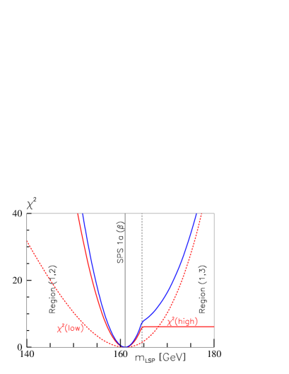
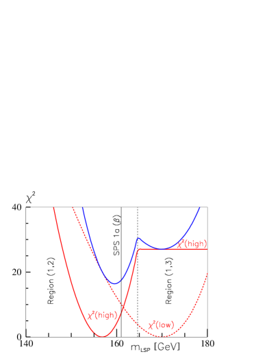
Figure 3: $\chi^{2}$ vs. $m_{{\tilde{\chi}^{0}_{1}}}$ (denoted $m_{\rm LSP}$). The other masses are held fixed. Left: nominal endpoint values; right: endpoint values off-set by $-20$ and $+15$ GeV.

If one allows also the other masses ($m_{{\tilde{q}_{L}}}$, $m_{{\tilde{\chi}^{0}_{2}}}$, $m_{{\tilde{l}_{R}}}$) to vary, the transition between regions (1,2) and (1,3) will move, and secondly, the minima will get deeper. In a more realistic analysis, however, the additional measurements of $m^{\rm max}_{qll}$ and, in particular $m^{\rm max}_{ll}$, will disfavor the second minimum. Indeed, with the additional information of the $qll$ “threshold”, this ambiguity was observed in the more detailed analysis reported in Gjelsten:2004ki . In Tables 3–4 we report on the probability of having false minima, and corresponding mass values, for SPS 1a ${(\alpha)}$ and ($\beta$).

Table 3: SPS 1a ${(\alpha)}$ ambiguities Gjelsten:2004ki . Left: Number of minima for $\Delta\chi^{2}<1$ (3) and their regions. Right: Minima for $\Delta\chi^{2}\leq 1$ in regions (1,1) and (1,2). Ensemble means, $\langle m\rangle$, and root-mean-square distances from the mean, $\sigma$, in GeV.

	$\#$ Minima	(1,1)	(1,2)
$\Delta\chi^{2}\leq 1$	1.12	94%	17%
$\Delta\chi^{2}\leq 3$	1.30	97%	33%

		(1,1)		(1,2)
	Nom	$\langle m\rangle$	$\sigma\hskip 6.45831pt$	$\langle m\rangle$	$\sigma\hskip 6.45831pt$
$m_{{\tilde{\chi}^{0}_{1}}}$	96.1	96.3	3.8	85.3	3.4
$m_{{\tilde{l}_{R}}}$	143.0	143.2	3.8	130.4	3.7
$m_{{\tilde{\chi}^{0}_{2}}}$	176.8	177.0	3.7	165.5	3.4
$m_{{\tilde{q}_{L}}}$	537.2	537.5	6.0	523.5	5.0

Table 4: Same as Table 3 but now for SPS 1a ${(\beta)}$. Without the $qll$ “threshold” two solutions were available, the nominal (1,2) low-mass one and a (1,1) high-mass one, see Fig. 2 (right panel). Due to the proximity of SPS 1a ${(\beta)}$ to the border between (1,2) and (1,3), with the inclusion of the threshold measurement a third solution has emerged. In the tables the high-mass solution (“hms”) is shown separately as it will probably be possible to discard it from other measurements. In the low-mass region there is either one solution, which can also lie on the border (“B”), or two.

		hms	1 solution	2 solutions
	$\#$ Min	(1,1)	(1,2)/(1,3)/B	(1,2)&(1,3)
$\Delta\chi^{2}\leq 1$	1.19	5%	82%	16%
$\Delta\chi^{2}\leq 3$	1.41	13%	72%	28%

		hms		1 solution		2 solutions
		(1,1)		(1,2)/(1,3)/B		(1,2)		(1,3)
	Nom	$\langle m\rangle$	$\sigma$	$\langle m\rangle$	$~{}~{}\sigma$	$\langle m\rangle$	$\sigma$	$\langle m\rangle$	$\sigma$
$m_{{\tilde{\chi}^{0}_{1}}}$	161	438	88	175	35	161	22	166	27
$m_{{\tilde{l}_{R}}}$	222	518	85	236	37	221	24	223	28
$m_{{\tilde{\chi}^{0}_{2}}}$	299	579	85	313	35	299	22	304	27
$m_{{\tilde{q}_{L}}}$	826	1146	104	843	44	826	30	835	36

IV LINEAR COLLIDER INPUT

With Linear Collider input on the LSP mass, taken to be determined with a precision of 0.05 GeV Aguilar-Saavedra:2001rg , the ambiguities are mostly resolved. For SPS 1a ${(\alpha)}$ the false solution is removed altogether. The masses and their errors are given in Table 5. For SPS 1a ${(\beta)}$ the high-mass solution no longer appears, but there is still an ambiguity in the low-mass region, see Table 6. These masses are however very close. Furthermore, as a Linear Collider will measure the slepton mass with an accuracy similar to that of the LSP mass Aguilar-Saavedra:2001rg , one may expect the remaining ambiguity to vanish as well. This possibility was not considered in the analyses Gjelsten:2004ki ; Gjelsten:2005aw and hence is not reflected in Tables 5–6.

Table 5: SPS 1a ${(\alpha)}$: Effect of adding a LC measurement of the LSP mass Gjelsten:2004ki .

		(1,1)
	Nom	$\langle m\rangle\$	$\sigma\hskip 4.30554pt$
$m_{{\tilde{\chi}^{0}_{1}}}$	96.05	96.05	0.05
$m_{{\tilde{l}_{R}}}$	142.97	142.97	0.29
$m_{{\tilde{\chi}^{0}_{2}}}$	176.82	176.82	0.17
$m_{{\tilde{q}_{L}}}$	537.25	537.2	2.5

Table 6: SPS 1a ${(\beta)}$: Effect of adding a LC measurement of the LSP mass.

		1 solution	2 solutions
	$\#$ Min	(1,2)/(1,3)/B	(1,2)&(1,3)
$\Delta\chi^{2}\leq 1$	1.21	79%	21%
$\Delta\chi^{2}\leq 3$	1.45	55%	45%

		1 solution		2 solutions
		(1,2)/(1,3)/B		(1,2)		(1,3)
	Nom	$\langle m\rangle$	$\sigma$	$\langle m\rangle$	$\sigma$	$\langle m\rangle$	$\sigma$
$m_{{\tilde{\chi}^{0}_{1}}}$	161.02	161.02	0.05	161.02	0.05	161.02	0.05
$m_{{\tilde{l}_{R}}}$	221.86	221.15	3.26	222.22	1.32	217.48	1.01
$m_{{\tilde{\chi}^{0}_{2}}}$	299.05	299.15	0.57	299.11	0.53	299.05	0.52
$m_{{\tilde{q}_{L}}}$	826.29	826.1	6.3	825.9	5.8	828.6	5.5

A second effect, not discussed above, is very clear by comparison of the errors on the masses obtained with and without the LC measurement: Fixing the LSP mass strongly reduces the errors on all the masses. This comes from the fact that the endpoint method determines mass differences much better than the actual masses themselves, a feature due to the way masses enter the endpoint expressions; in terms of differences of masses (squared). Actually, the errors on the masses obtained when the LHC and the LC are combined, Tables 5–6, are very close to the errors on the mass differences as obtained by the LHC alone.

The removal of ambiguities, and the higher precision are crucial for an extrapolation to the GUT scale Allanach:2004ud , a major goal of studying the spectroscopy of supersymmetric particles at future accelerators.

- (1) H. Baer, C. h. Chen, F. Paige and X. Tata, Phys. Rev. D 53 (1996) 6241 [arXiv:hep-ph/9512383]; I. Hinchliffe, F. E. Paige, M. D. Shapiro, J. Soderqvist and W. Yao, Phys. Rev. D 55 (1997) 5520 [arXiv:hep-ph/9610544]; I. Hinchliffe, F. E. Paige, E. Nagy, M. D. Shapiro, J. Soderqvist and W. Yao, LBNL-40954; H. Bachacou, I. Hinchliffe and F. E. Paige, Phys. Rev. D 62 (2000) 015009 [arXiv:hep-ph/9907518]; G. Polesello, Precision SUSY measurements with ATLAS for SUGRA point 5, ATLAS Internal Note, PHYS-No-111, October 1997.
- (2) B. C. Allanach, C. G. Lester, M. A. Parker and B. R. Webber, JHEP 0009 (2000) 004 [arXiv:hep-ph/0007009].
- (3) B. K. Gjelsten, D. J. Miller and P. Osland, JHEP 0412 (2004) 003 [arXiv:hep-ph/0410303].
- (4) B. C. Allanach et al., in Proc. of the APS/DPF/DPB Summer Study on the Future of Particle Physics (Snowmass 2001) ed. N. Graf, Eur. Phys. J. C 25 (2002) 113 [eConf C010630 (2001) P125] [arXiv:hep-ph/0202233].
- (5) B. K. Gjelsten, D. J. Miller and P. Osland, JHEP 0506 (2005) 015 [arXiv:hep-ph/0501033].
- (6) J. A. Aguilar-Saavedra et al. [ECFA/DESY LC Physics Working Group], arXiv:hep-ph/0106315.
- (7) B. C. Allanach, G. A. Blair, S. Kraml, H. U. Martyn, G. Polesello, W. Porod and P. M. Zerwas, arXiv:hep-ph/0403133.