Electroweak-Higgs Unification and the Higgs Boson Mass

Abstract

We propose an alternative unification scenario where the Higgs self-coupling ($\lambda$) is determined by impossing its unification with the electroweak gauge couplings. An attractive feature of models within this scenario is the possibility to determine the Higgs boson mass by evolving $\lambda$ from the electroweak-Higgs unification scale $M_{GH}$ down to the electroweak scale. The unification condition for the gauge ($g_{1},g_{2}$) and Higgs couplings is written as $g_{1}=g_{2}=f(\lambda)$, where $g_{1}=k_{Y}^{1/2}g_{Y}$, $k_{Y}$ being the normalization constant. Two variants for the unification condition are discussed; scenario I is defined through the linear relation: $g_{1}=g_{2}=k_{H}\lambda(M_{GH})$, while scenario II assumes a quadratic relation: $g^{2}_{1}=g^{2}_{2}=k_{H}\lambda(M_{GH})$. Fixing $k_{H}=O(1)$ and the standard normalization ($k_{Y}=5/3$), we obtain a Higgs boson mass value $m_{H}\simeq 190$ GeV, with similar results for other normalizations such as $k_{Y}=7/4$ and $3/2$. However, the unification scale $M_{GH}$ depends on the value of $k_{Y}$, going from $1.8\times 10^{12}$ GeV up to $4.9\times 10^{14}$ GeV for $7/4>k_{Y}>3/2$. Possible tests of this idea at a future Linear collider and its application for determining the Higgs spectrum in the Two-Higgs doublet model are also discussed. We also elaborate on these unification scenarios within the context of a six-dimensional $SU(3)_{c}\times SU(3)_{w}$ Gauge-Higgs unified model, where the Higgs boson arises as the extra-dimensional components of the 6D gauge fields.

I Introduction

The Standard Model (SM) of the strong and electroweak (EW) interactions has met with extraordinary success; it has been tested already at the level of quantum corrections radcorrs1 ; radcorrs2 . These corrections give some hints about the nature of the Higgs sector, pointing towards the existence of a relatively light Higgs boson, with a mass of the order of the EW scale, $m_{\phi_{SM}}\simeq v$ hixjenser . However, it is widely believed that the SM can not be the final theory of particle physics, in particular because the Higgs sector suffers from naturalness problems, and we really do not have a clear understanding of electroweak symmetry breaking (EWSB).

These problems in the Higgs sector can be stated as our present inability to find a satisfactory answer to some questions regarding its structure. In terms of the Higgs potential,

$$V(\Phi)=\mu^{2}_{0}\Phi^{\dagger}\Phi+\frac{\lambda}{4}(\Phi^{\dagger}\Phi)^{2}$$ (1)

these questions can be stated as follows:

1. What fixes the size (and sign) of the dimensionful parameter $\mu^{2}_{0}$?. This parameter determines the scale of EWSB in the SM; in principle it could be as high as the Planck mass, however it needs to be fixed to much lower values.

2. What is the nature of the quartic Higgs coupling $\lambda$?. This parameter is not associated with a known symmetry, and we expect all interactions in nature to be associated somehow with gauge forces, as these are the ones we understand better myghyunif .

An improvement on our understanding of EWSB is provided by the supersymmetric (SUSY) extensions of the SM softsusy , where loop corrections to the tree-level parameter $\mu^{2}_{0}$ are under control, thus making the Higgs sector more natural. The quartic Higgs couplings is nicely related with gauge couplings through relations of the form: $\lambda=\frac{1}{8}(g^{2}_{2}+g^{2}_{Y})$, thus solving this aspect of the problem too. In the SUSY alternative it is even possible to (indirectly) explain the sign of $\mu^{2}_{0}$ as a result loop effects and the breaking of the symmetry between bosons and fermions. Even if the Higgs mass parameter is taken to be positive at a high energy scale, renormalization effects drive its value negative at the EW scale, thus generating (explaining) EWSB.

Further progress to understand the SM structure is achieved in Grand Unified Theories (GUT), where the strong and electroweak gauge interactions are unified at a very high-energy scale ($M_{GUT}$) gutrev . However, certain consequences of the GUT idea seem to indicate that this unification, by itself, may be too violent (within the minimal SU(5) GUT model one actually gets inexact unification, too large proton decay, doublet-triplet problem, bad fermion mass relations, etc.), and some additional theoretical tool is needed to overcome these difficulties. Again, SUSY offers an amelioration of these problems. When SUSY is combined with the GUT program, one gets a more precise gauge coupling unification and some aspects of proton decay and fermion masses are under better control myradferm1 ; myradferm2 .

However, in order to verify the realization of SUSY-GUT in nature, it will take the observation of plenty of new phenomena such as superpartners, proton decay or rare decay modes. As nice as these ideas may appear, it seems worthwhile to consider other approaches for physics beyond the SM. For instance, it has been shown that additional progress towards understanding the SM origin, can be achieved by postulating the existence of extra dimensions. These theories have received much attention, mainly because of the possibility they offer to address the problems of the SM from a new geometrical perspective. These range from a new approach to the hierarchy problem ADD1 ; ADD2 ; ADD3 ; ADD4 ; RanSundrum up to a possible explanation of flavor hierarchies in terms of field localization along the extra dimensions nimashmaltz . Model with extra dimensions have been applied to neutrino physics abdeletal1 ; abdeletal2 ; abdeletal3 ; abdeletal4 , Higgs phenomenology myhixXD1 ; myhixXD2 , among many others. In the particular GUT context, it has been shown that it is possible to find viable solutions to the doublet-triplet problem hallnomu1 ; hallnomu2 . More recently, new methods in strong interactions have also been used as an attempt to revive the old models (TC, ETC, topcolor, etc) fathix . Other ideas have motivated new types of models as well (little Higgs littlehix , AdS/CFT composite Higgs models hixdual , etc).

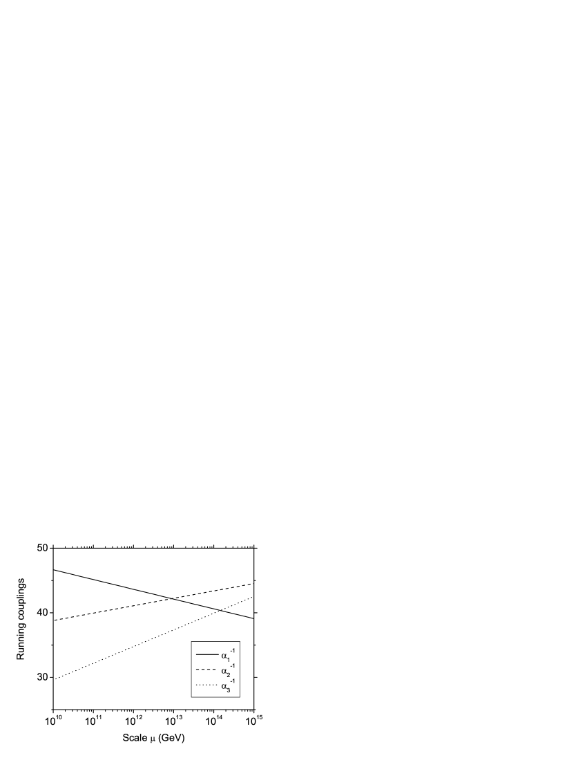
In this paper we are interested in exploring alternative unification scenarios, of weakly-interacting type, which could offer direct understanding of the Higgs sector too. We shall explore the consequences of a scenario where the electroweak $SU(2)_{L}\times U(1)_{Y}$ gauge interactions are unified with the Higgs self-interaction at an intermediate scale $M_{GH}$. Namely, we take seriously the indication of the running of the SM gauge couplings, which taken at face value (see Figure 1) show that the $U(1)$ and $SU(2)$ couplings approach first each other, before crossing with the strong coupling constant. Thus, we propose two variants for the unification condition which permit to predict the SM Higgs boson mass, with resulting values of the order $m_{H}\simeq 190$ GeV. The dependence of our results on the choice for the normalization for the hypercharge is also discussed, as well as possible test of this EW-Higgs unification idea at future colliders, such as ILC. We consider then (section III) the implementation of this idea in the two-Higgs doublet model, which allows to predict the Higgs spectrum, namely the masses for the neutral CP-even states ($h^{0},H^{0}$), the neutral CP-odd state ($A^{0}$) and the Charged Higgs ($H^{\pm}$). At this point it is relevant to compare our approach with the so called Gauge-Higgs unification program as they share some similarities. We think that our approach is more model independent, as we first explore the consequences of a parametric unification, without really choosing a definite model at higher energies. In fact, at higher energies both the SUSY models as well as the framework of extra dimensions could work as ultraviolet completion of our approach. The SUSY models could work because they allow to relate the scalar quartic couplings to the gauge couplings, thanks to the D-terms myghyunif . On the other hand, within the extra-dimensions it is also possible to obtain similar relations, when the Higgs fields are identified as the extra-dimensional components of gauge fields XDGHix1 ; XDGHix2 ; ABQuiros1 ; ABQuiros2 ; ABQuiros3 ; Hosotani1 ; Hosotani2 ; Hosotani3 ; Hosotani4 ; Hosotani5 ; Hosotani6 ; Hosotani7 ; Hosotani8 . Actually, we feel that the work of Ref.gauhixyuku1 ; gauhixyuku2 has a similar spirit to ours, in their case they look for gauge unification of the Higgs self-couplings that appear in the superpotential of NMSSM, and then they justify their work with a concrete model in 7D. Thus, in our case we also discuss the unification of the EW-Higgs couplings with the strong constant, which can be realized within the context of extra-dimensional Gauge-Higgs unified theories. In particular we discuss a 6D $SU(3)_{c}\times SU(3)_{w}$ model, which is broken on an orbifold $T^{2}/Z_{3}$ and the SM Higgs doublet is identified with the extra-dimensional components of the gauge fields.

Figure 1: Evolution of the running couplings as functions of the scale $\mu$ in the context of the SM, taking $m_{top}=170.0$ GeV.

Figure 2: Prediction for the Higgs boson mass as a function of $k_{H}$ in the context of the SM with $k_{Y}=5/3$, in the frame of scenario I, taking $m_{top}=165.0;\,167.5;\,170.0;\,172.5;\,175.0$ GeV.

Figure 3: Prediction for the Higgs boson mass as a function of $k_{H}$ in the context of the SM with $k_{Y}=5/3$, in the frame of scenario II, taking $m_{top}=165.0;\,167.5;\,170.0;\,172.5;\,175.0$ GeV.

Figure 4: Prediction for the Higgs boson mass as a function of $k_{H}$ in the context of the SM with $k_{Y}=3/2$, in the frame of scenario I, taking $m_{top}=165.0;\,167.5;\,170.0;\,172.5;\,175.0$ GeV.

II Gauge-Higgs unification in the SM

In the present EW-Higgs unified scenario, we shall assume that there exists a scale where the gauge couplings constants $g_{1},g_{2}$, associated with the gauge symmetry $SU(2)_{L}\times U(1)_{Y}$, are unified, and that at this scale they also get unified with the Higgs self coupling $\lambda$, i.e. $g_{1}=g_{2}=f(\lambda)$ at $M_{GH}$. The precise relation between $g_{1}$ and $g_{Y}$ (the SM hypercharge coupling) involves a normalization factor $k_{Y}$, i.e. $g_{1}=k_{Y}^{1/2}g_{Y}$, which depends on the unification model. The standard normalization gives $k_{Y}=5/3$, which is associated with minimal models such as $SU(5),SO(10),E_{6}$. However, in the context of string theory it is possible to have such standard normalization without even having a unification group. For other unification groups that involve additional $U(1)$ factors, one would have exotic normalizations too, and similarly for the case of GUT models in extra-dimensions. In what follows we shall present results for the cases: $k_{Y}=5/3,3/2$ and $7/4$, which indeed arise in string-inspired models Dienes:1996yh . Note that these values fall in the range $3/2<5/3<7/4$ and so they can illustrate what happens when one chooses a value below or above the standard normalization. The form of the unification condition will depend on the particular realization of this scenario, which could be as generic as possible. However, in order to be able to make predictions for the Higgs boson mass, we shall consider two specific realizations. Scenario I will be based on the linear relation: $g_{2}=g_{1}=k_{H}\lambda(M_{GH})$, where the factor $k_{H}$ is included in order to retain some generality, for instance to take into account possible unknown group theoretical or normalization factors. Motivated by specific models, such as SUSY itself, as well as an argument based on the power counting of the beta coefficients in the RGE for scalar couplings, namely the fact that $\beta_{\lambda}$ goes as $O(g^{4})$, we shall also define scenario II, through the quadratic unification condition: $g^{2}_{1}=g^{2}_{2}=k_{H}\lambda(M_{GH})$.

The SM renormalization group equations at the one loop level involving the gauge coupling constants $g_{1,2,3}$, the Higgs self-coupling $\lambda$, the top-quark Yukawa coupling $g_{t}$, and the parameter $k_{Y}$, can be written as follows rgebsm ; langa1 :

$$\frac{dg_{i}}{dt} = \frac{b_{i}^{sm}}{16\pi^{2}}g^{3}_{i}\ ,$$ (2)

$$\frac{dg_{t}}{dt} = \frac{g_{t}}{16\pi^{2}}\left[\frac{9}{2}g^{2}_{t}-\left(\frac{17}{12k_{Y}}g^{2}_{1}+\frac{9}{4}g^{2}_{2}+8g^{2}_{3}\right)\right]\ ,$$ (3)

$$\frac{d\lambda}{dt} = \frac{1}{16\pi^{2}}\left[12\lambda^{2}-\left(\frac{3}{k_{Y}}g^{2}_{1}+9g^{2}_{2}\right)\lambda+\frac{9}{4}\left(\frac{1}{3k_{Y}^{2}}g^{4}_{1}+\frac{2}{5}g^{2}_{1}g^{2}_{2}+g^{4}_{2}\right)+12g^{2}_{t}\lambda-12g^{4}_{t}\right]\ ,$$ (4)

where $(b_{1}^{sm},b_{2}^{sm},b_{3}^{sm})=(41/6k_{Y},-19/6,-7)$; $\mu$ denotes the scale at which the coupling constants are defined, and $t=\log(\mu/\mu_{0})$. The corresponding expressions for the SM renormalization group equations at the two-loop level can be found in Ref. langa1 .

Now, we discuss the predictions for the Higgs boson mass and its dependence on the parameter $k_{H}$. In practice, we determine first the scale $M_{GH}$ at which $g_{2}$ and $g_{1}$ are unified, then we fix the quartic Higgs coupling $\lambda$ by imposing the unification condition and finally, by evolving the quartic Higgs coupling down to the EW scale, we are able to predict the Higgs boson mass. For the numerical calculations, to be discussed next, we employ the full two-loop SM renormalization group equations involving the gauge coupling constants $g_{1,2,3}$, the Higgs self-coupling $\lambda$, the top-quark Yukawa coupling $g_{t}$, and the parameter $k_{Y}$ rgebsm ; langa1 . We also take the values for the coupling constants as reported in the Review of Particle Properties revPP , while for the top quark mass we take the value recently reported in lasttopm1 ; lasttopm2 .

In order to get a flavor of the coupling constants behavior and evolution, we find it convenient to discuss first an analytical solution based on the one-loop beta-functions for the gauge couplings (Eqs. (2),(3)), while for the Higgs self-coupling (Eq. (4)) we will only keep the term proportional to $\lambda$ itself, and work with the canonical normalization $k_{Y}=5/3$. In this case, the solution for the gauge coupling constants takes the form:

$$\frac{1}{g^{2}_{i}(\mu)}=\frac{1}{g^{2}_{i}(\mu_{0})}-2\frac{b_{i}}{16\pi^{2}}(t-t_{0})$$ (5)

Then, from the unification condition $g_{2}(M_{GH})=g_{1}(M_{GH})$, we get the value: $M_{GH}=1.086\times 10^{13}$ GeV. Solving the equation for $\lambda$, we obtain:

$$\frac{1}{\lambda(\mu)}=\frac{1}{\lambda(M_{GH})}+\frac{3}{4\pi^{2}}ln(M_{GH}/\mu)$$ (6)

Then, using the relation $g_{2}(M_{GH})=g_{1}(M_{GH})=k_{H}\lambda(M_{GH})$ from Scenario I, with $k_{H}=1$, we get the value of $\lambda$ at low energies, i.e. for $\mu=m_{Z}$, it is $\lambda(m_{Z})=0.39$, which implies a Higgs boson mass of $m_{H}=219$ GeV. This value is indeed of the order of the EW scale and the result looks quite encouraging.

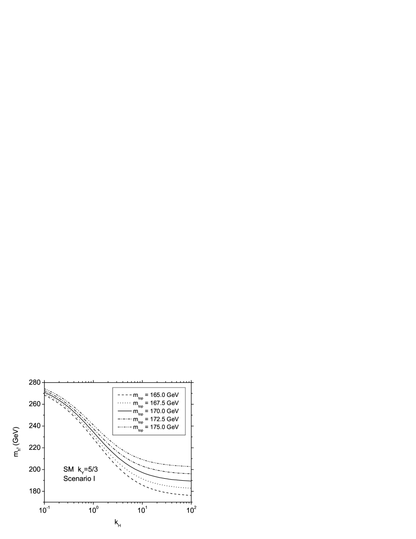
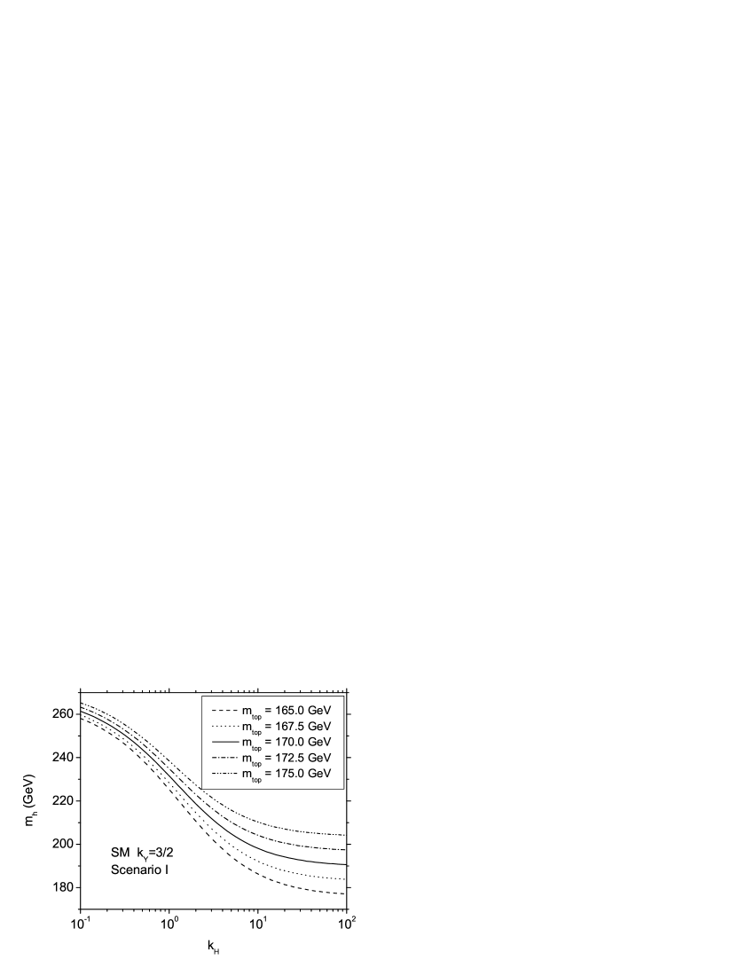
Now, let us discuss first the results of the full numerical analysis for $k_{Y}=5/3$, for which we find that $M_{GH}\cong 1.0\times 10^{13}$ GeV. Figures 2 and 3 show the prediction for the Higgs boson mass in scenarios I and II, respectively. The Higgs boson mass is shown as function of the parameter $k_{H}$ over a range $10^{-1}<k_{H}<10^{2}$, which covers three orders of magnitude and hopefully illustrates the generality of our results. We want to point out here that the expected natural value for $k_{H}$ is 1.

For such a range of $k_{H}$, the Higgs boson mass takes the values: $176<m_{H}<275$ GeV for scenario I, while for $k_{H}=1$ we obtain a prediction for the Higgs boson mass: $m_{H}=229,\,234,\,241$ GeV, for a top quark mass of $m_{top}=165,\,170,\,175$ GeV lasttopm1 ; lasttopm2 , respectively. On the other hand, for scenario II, we find that the Higgs boson mass can take the values: $175<m_{H}<269$ GeV, while for $k_{H}=1$ we obtain: $m_{H}=214,\,222,\,230$ GeV.

Then, when we compare our results with the Higgs boson mass obtained from EW precision measurements, which imply $m_{H}\lower 3.01385pt\hbox{$\;\stackrel{{\scriptstyle\textstyle<}}{{\sim}}\;$}190$ GeV, we notice that in order to get compatibility with such value, our model seems to prefer high values of $k_{H}$. For instance, by taking the lowest value that we consider here for the top mass, $m_{t}=165$ GeV, and fixing $k=10^{2}$, we obtain the minimum value for the Higgs boson mass equal to $m_{H}=176$ GeV in scenario I, while scenario II implies a slightly minimal lower value, namely $m_{H}=175$ GeV.

In turn, Figures 4 and 5, show the results for the Higgs boson mass using the value $k_{Y}=3/2$, for which we find that $M_{GH}=4.9\times 10^{14}$ GeV, somehow higher than the previous case, but for which one still gets a mass gap between $M_{GH}$ and a possible $M_{GUT}$. One finds somehow higher values for the Higgs boson mass, for instance for $k_{H}=1$, one gets $m_{H}=225,\,232,\,238$ ($m_{H}=212,\,220,\,218$) GeV for scenarios I (II).

On the other hand, Figures 6 and 7, show the results for the Higgs boson mass using the value $k_{Y}=7/4$, for which we find that $M_{GH}=1.8\times 10^{12}$ GeV, which is lower than the one of the previous cases, and has an even larger mass gap between $M_{GH}$ and a possible $M_{GUT}$. One finds somehow higher values for the Higgs boson mass, for instance for $k_{H}=1$, one gets $m_{H}=230,\,236,\,243$ ($m_{H}=215,\,223,\,231$) GeV for scenarios I (II).

At this point, rather than continuing discussions on the precise Higgs boson mass, we would like to emphasize that our approach based on the EW-Higgs unification idea is very successful in giving a Higgs boson mass that has indeed the correct order of magnitude, and that once measured at the LHC we will be able to fix the parameter $k_{H}$ and find connections with other approaches for physics beyond the SM, such as the one to be discussed next.

In fact, for the Higgs boson mass range that is predicted in our approach, it turns out that the Higgs will decay predominantly into the mode $h\to ZZ$, from which there are good chances to meassure the Higgs boson mass with a precision of the order $5\%$ Duhrssen:2004cv1 ; Duhrssen:2004cv2 , therefore it will make possible to bound $k_{H}$ to within the few percent level. Further tests of our EW-Higgs unification hypothesis would involve testing more implications of the quartic Higgs coupling. For instance one could use the production of Higgs pairs ($e^{+}e^{-}\to\nu\overline{\nu}hh$) at a future linear collider, such as the ILC. This is just another example of the complementarity of future studies at LHC and ILC.

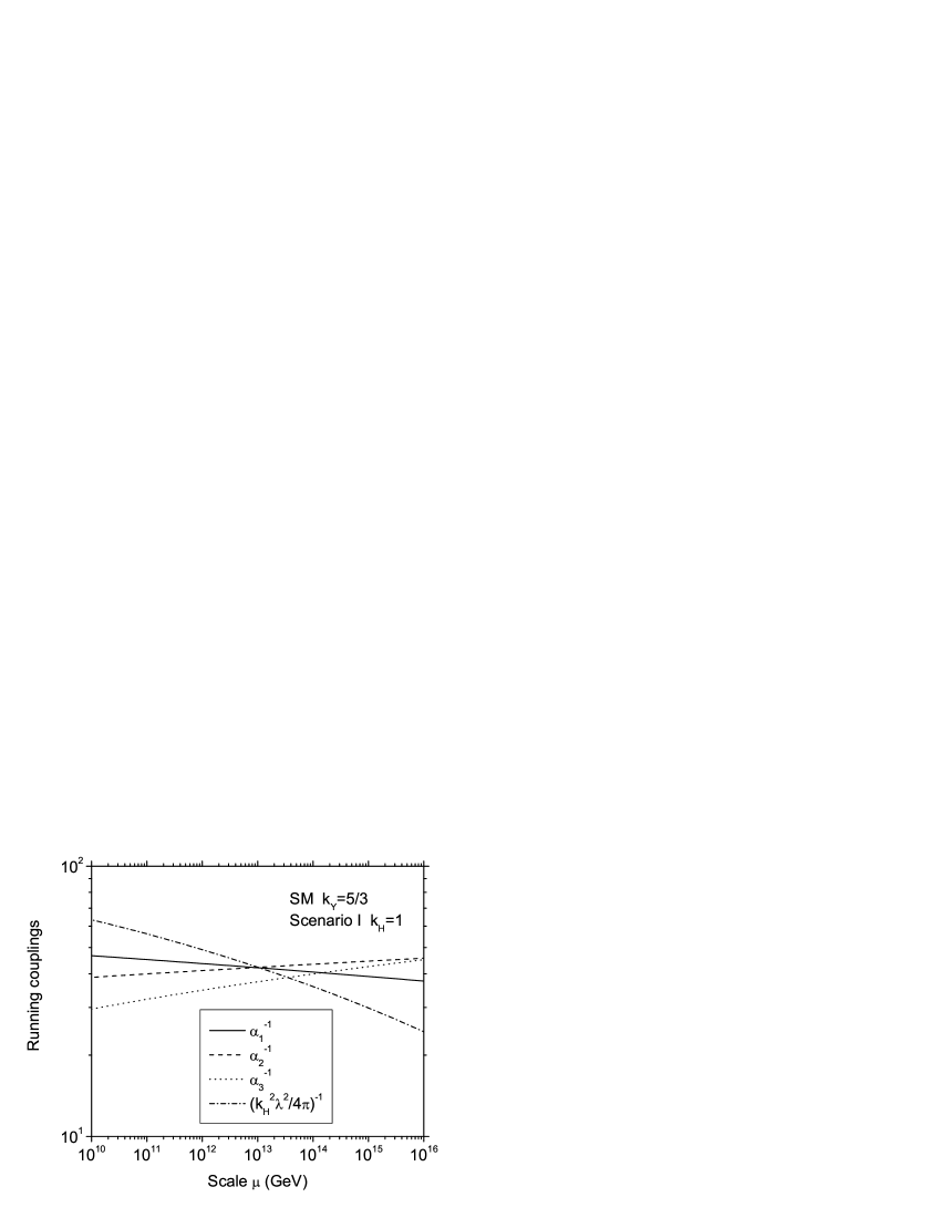
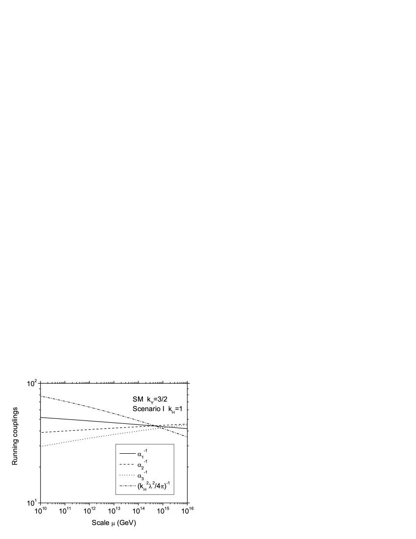
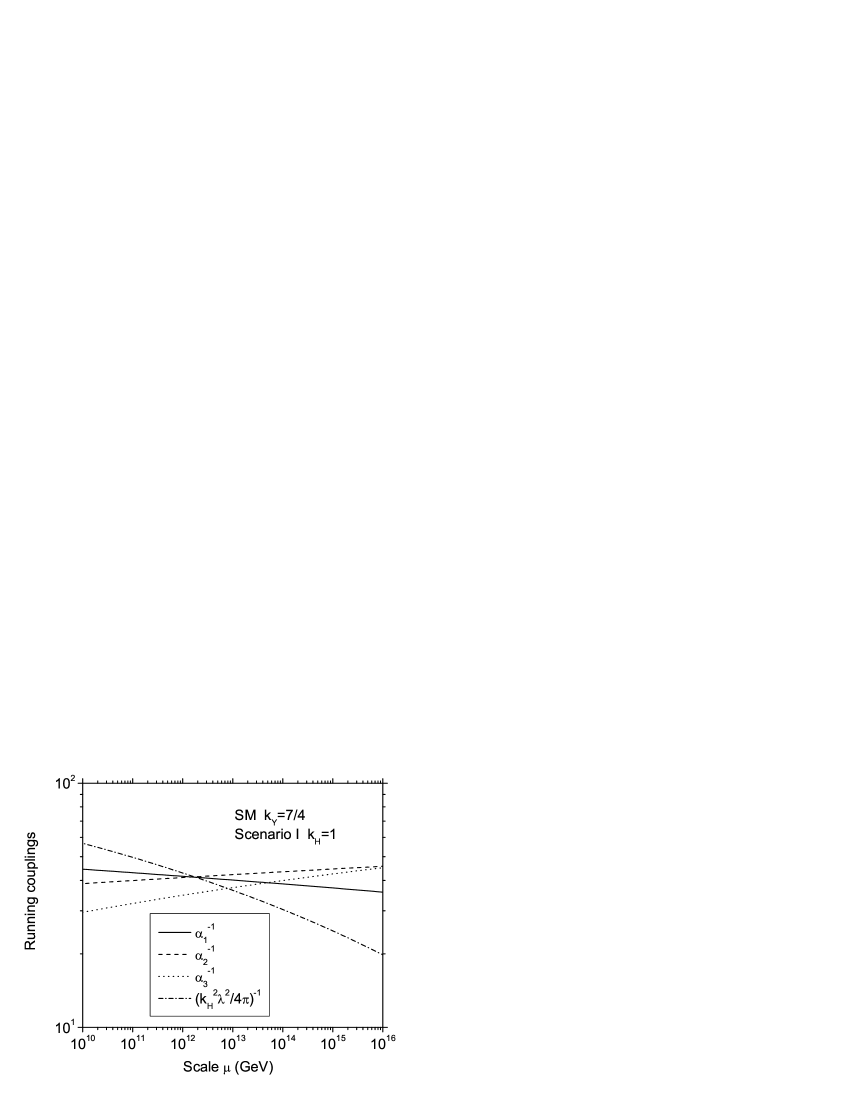
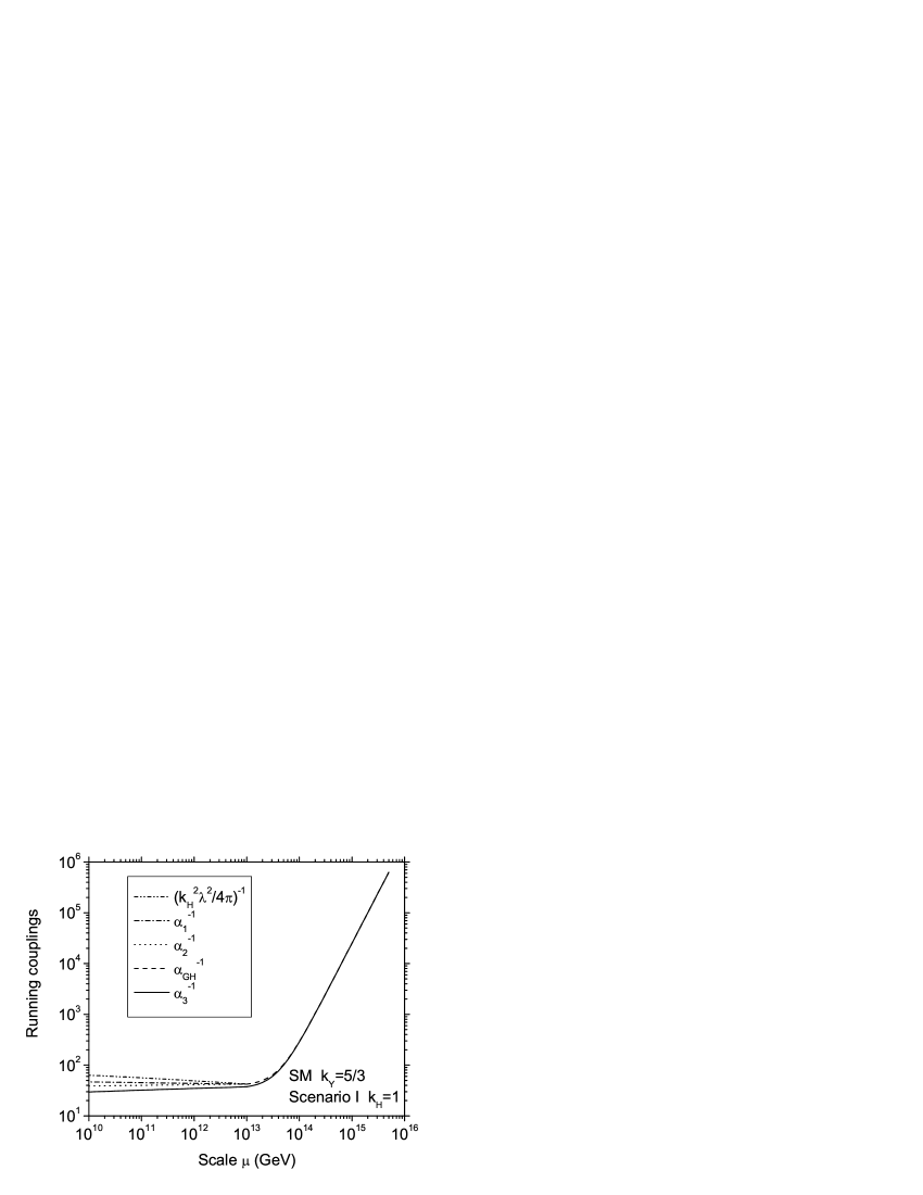
To end this section, we show the evolution of the running couplings

$$\alpha_{i}^{-1}=\left(\frac{g_{i}^{2}}{4\pi}\right)^{-1}\,\,\,(i=1,2,3)\,,\,\,\,\mbox{and}\,\,\left(\frac{k_{H}^{2}\,\lambda^{2}}{4\pi}\right)^{-1}\,,$$ (7)

as functions of the scale $\mu$ in the context of the SM for $k_{Y}=5/3$, $k_{Y}=3/2$, and $k_{Y}=7/4$ in Figures 8, 9, 10, respectively. We perform the numerical calculations in the frame of scenario I with $k_{H}=1$ and taking $m_{top}=170.0$ GeV. In these Figures the EW couplings $g_{1,2}$ unify at the scale $M_{GH}$ and by assumption so does the Higgs self-coupling $\lambda$. We notice that in all these cases, the scale $M_{GH}$ is clearly below the usual GUT Scale, thus signaling the viability of our assumption of EW-Higgs unification.

III EW-Higgs unification in the Two-Higgs doublet model.

In the two-Higgs doublet model (THDM), one includes two scalar doublets ($\Phi_{1}$, $\Phi_{2}$) in the Higgs sector. The Higgs potential can be written as follows thdmky :

$$V(\Phi_{1},\Phi_{2}) = \mu^{2}_{1}\Phi_{1}^{\dagger}\Phi_{1}+\mu^{2}_{2}\Phi_{2}^{\dagger}\Phi_{2}+\lambda_{1}(\Phi_{1}^{\dagger}\Phi_{1})^{2}+\lambda_{2}(\Phi_{2}^{\dagger}\Phi_{2})^{2}+\lambda_{3}(\Phi_{1}^{\dagger}\Phi_{1})(\Phi_{2}^{\dagger}\Phi_{2})$$ (8)

$$+\lambda_{4}(\Phi_{1}^{\dagger}\Phi_{2})(\Phi_{2}^{\dagger}\Phi_{1})+\frac{1}{2}\lambda_{5}[(\Phi_{1}^{\dagger}\Phi_{2})^{2}+(\Phi_{2}^{\dagger}\Phi_{1})^{2}]\ .$$

One can observe that by absorbing a phase in the definition of $\Phi_{2}$, one can make $\lambda_{5}$ real and negative, which pushes all potential CP violating effects into the Yukawa sector:

$$\lambda_{5}\leq 0.$$ (9)

In order to avoid spontaneous breakdown of the electromagnetic $U(1)$ loren1 , the vacuum expectation values must have the following form:

$$\langle\Phi_{1}\rangle=\left(\begin{array}[]{c}0\\ v_{1}\end{array}\right)\,\,\,,\,\,\,\langle\Phi_{2}\rangle=\left(\begin{array}[]{c}0\\ v_{2}\end{array}\right)\,\,\,,$$ (10)

$v_{1}^{2}+v_{2}^{2}\equiv v^{2}=(246GeV)^{2}$. This configuration is indeed a minimum of the tree level potential if the following conditions are satisfied.

$$\lambda_{1} \geq 0\ ,$$

$$\lambda_{2} \geq 0\ ,$$

$$\lambda_{4}+\lambda_{5} \leq 0\ ,$$

$$4\lambda_{1}\lambda_{2} \geq (\lambda_{3}+\lambda_{4}+\lambda_{5})^{2}\ .$$ (11)

The scalar spectrum in this model, includes two CP-even states ($h^{0},H^{0}$), one CP-odd ($A^{0}$) and two charged Higgs bosons ($H^{\pm}$). The tree level expressions for the masses and mixing angles are given as follows:

$$\tan\beta = \frac{v_{2}}{v_{1}}\ ,$$ (12)

$$\sin\alpha = -(\mbox{sgn}\,C)\left[\frac{1}{2}\frac{\sqrt{(A-B)^{2}+4C^{2}}-(B-A)}{\sqrt{(A-B)^{2}+4C^{2}}}\right]^{1/2}\ ,$$ (13)

$$\cos\alpha = \left[\frac{1}{2}\frac{\sqrt{(A-B)^{2}+4C^{2}}+(B-A)}{\sqrt{(A-B)^{2}+4C^{2}}}\right]^{1/2}\ ,$$ (14)

$$M^{2}_{H^{\pm}} = -\frac{1}{2}(\lambda_{4}+\lambda_{5})v^{2}\ ,$$ (15)

$$M^{2}_{A^{0}} = -\lambda_{5}v^{2}\ ,$$ (16)

$$M^{2}_{H^{0},h^{0}} = \frac{1}{2}\left[A+B{\pm}\sqrt{(A-B)^{2}+4C^{2}}\right]\ ,$$ (17)

where $A=2\lambda_{1}v^{2}_{1}$, $B=2\lambda_{2}v^{2}_{2}$, $C=(\lambda_{3}+\lambda_{4}+\lambda_{5})v_{1}v_{2}$.

The two Higgs doublet models are described by 7 independent parameters which can be taken to be $\alpha$, $\beta$, $M_{H^{\pm}}$, $M_{H^{0}}$, $M_{h^{0}}$, $M_{A^{0}}$, while the top quark mass given by:

$$M_{t}=g_{t}v\sin\beta\ .$$ (18)

Now, we write the THDM renormalization group equations at the one loop level involving the gauge coupling constants $g_{1,2,3}$, the Higgs self-couplings $\lambda_{1,2,3,4,5}$, the top-quark Yukawa coupling $g_{t}$, and the parameter $k_{Y}$, as follows thdmky ; langa1 :

$$\frac{dg_{i}}{dt} = \frac{b_{i}^{thdm}}{16\pi^{2}}g^{3}_{i}\ ,$$ (19)

$$\frac{dg_{t}}{dt} = \frac{g_{t}}{16\pi^{2}}\left[\frac{9}{2}g^{2}_{t}-\left(\frac{17}{12k_{Y}}g^{2}_{1}+\frac{9}{4}g^{2}_{2}+8g^{2}_{3}\right)\right]\ ,$$ (20)

$$\frac{d\lambda_{1}}{dt} = \frac{1}{16\pi^{2}}\left[24\lambda_{1}^{2}+2\lambda_{3}^{2}+2\lambda_{3}\lambda_{4}+\lambda_{5}^{2}+\lambda_{4}^{2}-3\lambda_{1}(3g^{2}_{2}+\frac{1}{k_{Y}}g^{2}_{1})+12\lambda_{1}g^{2}_{t}\right.$$ (21)

$$\left.+\frac{9}{8}g^{4}_{2}+\frac{3}{4k_{Y}}g^{2}_{1}g^{2}_{2}+\frac{3}{8k^{2}_{Y}}g^{4}_{1}-6g^{4}_{t}\right]\ ,$$

$$\frac{d\lambda_{2}}{dt} = \frac{1}{16\pi^{2}}\left[24\lambda_{2}^{2}+2\lambda_{3}^{2}+2\lambda_{3}\lambda_{4}+\lambda_{5}^{2}+\lambda_{4}^{2}-3\lambda_{2}(3g^{2}_{2}+\frac{1}{k_{Y}}g^{2}_{1})\right.$$ (22)

$$\left.+\frac{9}{8}g^{4}_{2}+\frac{3}{4k_{Y}}g^{2}_{1}g^{2}_{2}+\frac{3}{8k^{2}_{Y}}g^{4}_{1}\right]\ ,$$

$$\frac{d\lambda_{3}}{dt} = \frac{1}{16\pi^{2}}\left[4(\lambda_{1}+\lambda_{2})(3\lambda_{3}+\lambda_{4})+4\lambda^{2}_{3}+2\lambda^{2}_{4}+2\lambda_{5}^{2}-3\lambda_{3}(3g^{2}_{2}+\frac{1}{k_{Y}}g^{2}_{1})\right.$$ (23)

$$\left.+6\lambda_{3}g^{2}_{t}+\frac{9}{4}g^{4}_{2}-\frac{3}{2k_{Y}}g^{2}_{1}g^{2}_{2}+\frac{3}{4k^{2}_{Y}}g^{4}_{1}\right]\ ,$$

$$\frac{d\lambda_{4}}{dt} = \frac{1}{16\pi^{2}}\left[4\lambda_{4}(\lambda_{1}+\lambda_{2}+2\lambda_{3}+\lambda_{4})+8\lambda_{5}^{2}-3\lambda_{4}(3g^{2}_{2}+\frac{1}{k_{Y}}g^{2}_{1})\right.$$ (24)

$$\left.+6\lambda_{4}g^{2}_{t}+\frac{3}{k_{Y}}g^{2}_{1}g^{2}_{2}\right]\ ,$$

$$\frac{d\lambda_{5}}{dt} = \frac{1}{16\pi^{2}}\left[\lambda_{5}\left((4\lambda_{1}+4\lambda_{2}+8\lambda_{3}+12\lambda_{4}+8\lambda_{5}^{2}-3(3g^{2}_{2}+\frac{1}{k_{Y}}g^{2}_{1})+6g^{2}_{t}\right)\right]\ ,$$ (25)

where $(b_{1}^{thdm},b_{2}^{thdm},b_{3}^{thdm})=(7/k_{Y},-3,-7)$; $\mu$ denotes the scale at which the coupling constants are defined, and $t=\log(\mu/\mu_{0})$.

The form of the unification condition will depend on the particular realization of this scenario, which could be as generic as possible. However, in order to be able to make predictions for the Higgs mass, we shall consider again two specific realizations. Scenario I will be based on the linear relation:

$$g_{1}=g_{2}=k_{H}(i)\,\lambda_{i}(M_{GH})\hskip 71.13188pt(i=1,2,3,4,5)\,,$$ (26)

where the factors $k_{H}(i)$ are included in order to take into account possible unknown group theoretical or normalization factors. We shall also define scenario II, which uses quadratic unification conditions; as follows:

$$g^{2}_{1}=g^{2}_{2}=k_{H}(i)\,\lambda_{i}(M_{GH})\hskip 71.13188pt(i=1,2,3,4,5)\,.$$ (27)

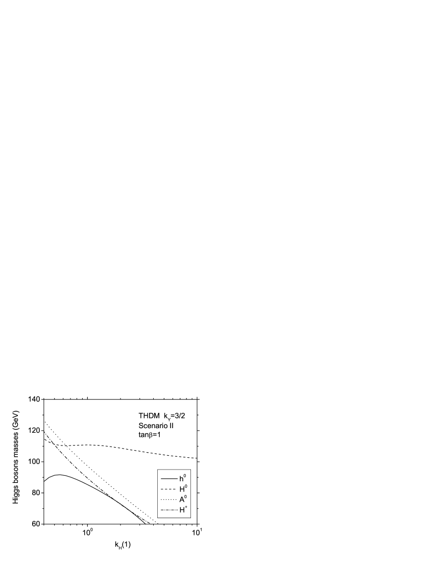
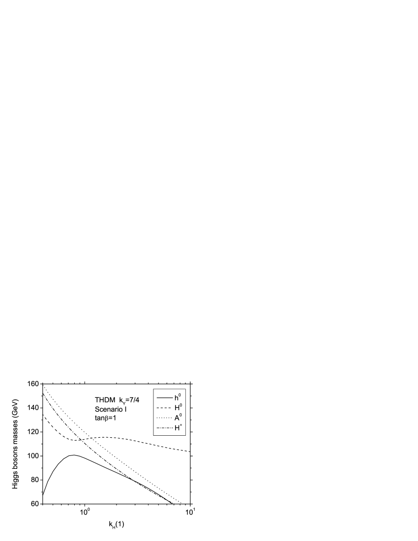
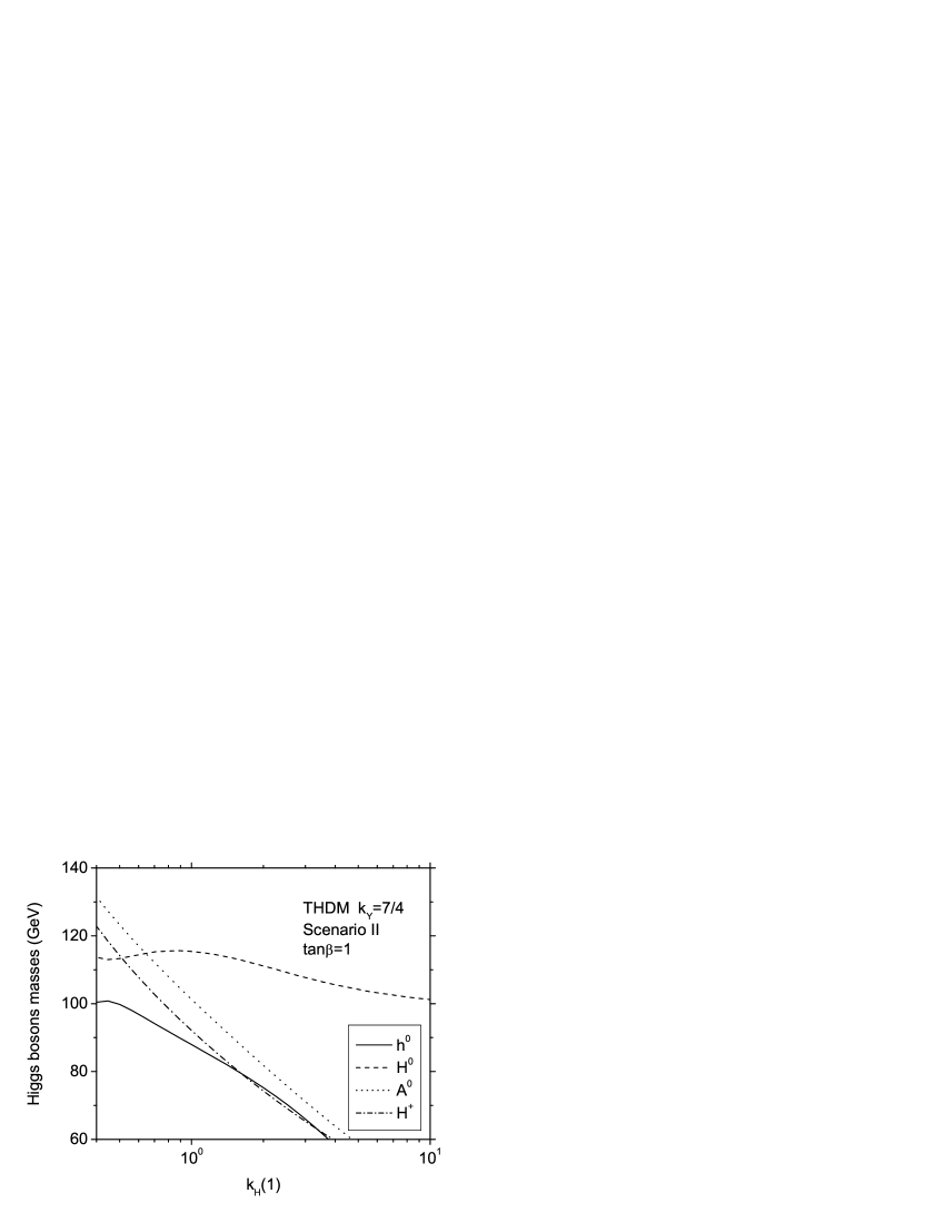
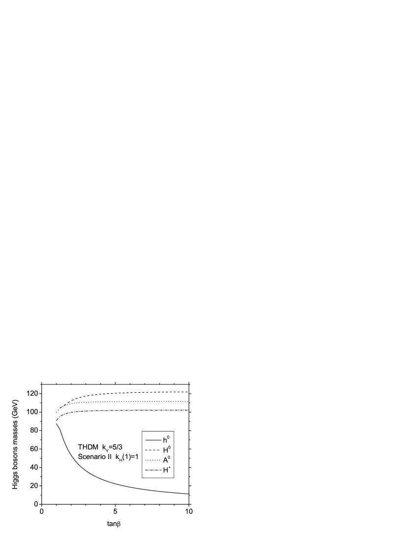
Now, we present first the results of the numerical analysis for the Higgs bosons masses in the context of the two Higgs-doublet model for $\tan\beta=1$ and taking $m_{top}=170.0$ GeV. In order to get an idea of the behavior of the masses of the Higgs bosons ($h^{0}$, $H^{0}$, $A^{0}$, $H^{\pm}$) we make the following choice ad hoc:

$$-k_{H}(5)=-\frac{1}{3}k_{H}(4)=3k_{H}(3)=k_{H}(2)=k_{H}(1)\,,$$ (28)

for both scenarios I and II. The Higgs bosons masses are shown as functions of the parameter $k_{H}$ over a range $0.1<k_{H}<10$, which covers two orders of magnitude and hopefully illustrates the generality of our results.

Now, let us discuss first the results of the full numerical analysis for $k_{Y}=5/3$, for which we find that $M_{GH}=1.3\times 10^{13}$ GeV. In Figures 11 and 12 we show the prediction for the Higgs bosons masses as functions of $k_{H}(1)$ for $k_{Y}=5/3$, in the frame of scenarios I and II, respectively.

For such a range of $k_{H}(1)$, the mass of the Higgs boson $h^{0}$ takes the values: $m_{h^{0}}<98$ GeV for scenario I, while for $k_{H}(1)=1$ we obtain a prediction for the Higgs boson mass: $m_{h^{0}}=97$ GeV. On the other hand, for scenario II, we find that the Higgs boson mass can take the values: $m_{h^{0}}<98$ GeV, while for $k_{H}(1)=1$ we obtain: $m_{h^{0}}=88$ GeV.

In turn, Figures 13 and 14, show the results for the Higgs boson mass using the value $k_{Y}=3/2$, for which we find that $M_{GH}=5.9\times 10^{14}$ GeV, somehow higher than the previous case, but for which one still gets a mass gap between $M_{GH}$ and a possible $M_{GUT}$. One finds somehow lower values for the Higgs boson mass, for instance for $k_{H}(1)=1$, one gets $m_{h^{0}}=92$ (85) GeV for scenarios I (II).

On the other hand, Figures 15 and 16, show the results for the Higgs boson mass using the value $k_{Y}=7/4$, for which we find that $M_{GH}=2.2\times 10^{12}$ GeV, which is lower than the one of the previous cases, and has an even larger mass gap between $M_{GH}$ and a possible $M_{GUT}$. One finds somehow higher values for the Higgs boson mass, for instance for $k_{H}(1)=1$, one gets $m_{h^{0}}=98$ (88) GeV for scenarios I (II).

As can be seen from these figures, for lower values of $\tan\beta$ one gets an irregular behavior of the other Higgs masses, while for higher values of $\tan\beta$, there is an approximate degeneracy, with all masses in the range of $100-120$ GeV. Finally, we want to put emphasis on the following. Even though the analysis of the EW-Higgs Unification within the THDM implies that the lightest neutral CP-even Higgs boson has a mass ($\sim 80$ GeV) that is somehow below the LEP bounds, 114.4 GeV unknown:2006cr ; Barate:2003sz , it should be mentioned that this bound refers to the SM Higgs boson. The bound on the lightest Higgs boson of the THDM depends on the factor $\sin^{2}(\beta-\alpha)$, which could be less than 1, and thus results in weaker Higgs boson mass bounds. We have estimated this factor within our approach and we obtain typical values in the range $0.01\leq\sin^{2}(\alpha-\beta)\leq 0.8$, (see Table 1) which means that those LEP bounds do not necessarily apply. In fact, we can make use of the experimental results reported in the Table 14 of Ref.unknown:2006cr which allow assuming SM decay rates a simple and direct check of our model results. After this comparison we observe that only the first four points in our Table I survive. Even though that the parameter space is drastically reduced, this shows that there is still an allowed region which deserves future detailed investigations. We end this section saying that for the THDM case our model seems to prefer values of $k_{H}\lower 3.01385pt\hbox{$\;\stackrel{{\scriptstyle\textstyle<}}{{\sim}}\;$}1$.

IV EW-Higgs and Extended GUT within extra-dimensions.

We shall show in this section that it is possible to make further progress: to achieve a Grand Unification of all the coupling constants at an scale $M_{GUT}>M_{GH}$, and to justify the EW-Higgs unification. All we need to do is to consider an extra-dimensional setting.

We have already shown the evolution of the coupling constants in Figures 8, 9 and 10. The EW couplings $g_{1,2}$ unify at the scale $M_{GH}$ and by assumption so does the Higgs self-coupling $\lambda$. Above $M_{GH}$ we shall assume that $g_{1,2}$ and $\lambda$ evolve as a single unified coupling $g_{H}$. However, to determine its evolution, we need to assume some particular way of embedding the groups $SU(2)_{L}$ and $U(1)_{Y}$ into some unified gauge group, $G_{WH}$. Although it is possible to construct 4D models where such unification can be achieved, we also want to justify our assumption of EW-Higgs unification and, at present, the most promising approach seems to be the Gauge-Higgs unification in extra-dimensions. Furthermore, in order to search for a complete unification of $g_{H}$ with the strong coupling constant $g_{3}$, we also need to assume what kind of physics exists above $M_{GH}$ for the QCD sector.

Here is where extra-dimensions will play a prominent role. We assume that above $M_{GH}$ the window into a pair of extra-dimensions opens up. Thus, both the strong and the EW-Higgs couplings will run from $M_{GH}$ up to another unification scale $M_{GUT}$, with the typical power-like behavior of extra-dimensional running of the coupling constants. Furthermore, the extra-dimensional (XD) framework provides a possible explanation for the EW-Higgs unification. Namely, we shall identify the Higgs boson as a component of the XD gauge field XDGHix1 ; XDGHix2 . Promising models could be constructed in five and six dimensions, with or without SUSY ABQuiros1 ; ABQuiros2 ; ABQuiros3 ; Hosotani1 ; Hosotani2 ; Hosotani3 ; Hosotani4 ; Hosotani5 ; Hosotani6 ; Hosotani7 ; Hosotani8 . Unification of Higgs and matter with the gauge multiplets has also been discussed gauhixyuku1 ; gauhixyuku2 .

To build a model based on the idea of gauge-Higgs unification in extra-dimensions, we consider a 6D $SU(3)_{c}\times SU(3)_{W}$ gauge theory compactified on a $T^{2}/Z_{n}$ orbifold. For $Z_{n}=Z_{2}$ one gets two Higgs doublets in the spectrum of zero modes, while for $Z_{n}=Z_{3}$ one gets only one Higgs doublet. Here we shall consider the case $Z_{3}$ for definitness. The 6D gauge bosons are $A_{M}=T^{A}A^{A}_{M}$ [$M=(\mu,i)$, with $i=5,6$]. The full gauge symmetry is broken by the orbifold boundary conditions (O.B.C.):

$$A_{\mu}(x_{\mu},y)\to A_{\mu}(x_{\mu},-y) = +PA_{\mu}(x_{\mu},y)P^{-1},$$

$$A_{i}(x_{\mu},y)\to A_{i}(x_{\mu},-y) = -PA_{i}(x_{\mu},y)P^{-1},$$ (29)

where $P=diag(1,1,-1)$ acts on gauge space as an “inner automorphism”, such that the gauge symmetry can be broken as: $G\to H$, with $H=SM$. Thus, O.B.C. split the group generators into two sets, $T^{A}=\{T^{a},T^{k}\}$, $T^{A}\,\epsilon\,G$, $T^{a}\,\epsilon\,H$. Since $A^{a}_{\mu}$ has even $Z_{2}-$ parity, it has zero modes in the spectrum. On the other hand, $A^{k}_{\mu}$ has odd $Z_{2}-$ parity, and does not have zero modes in the spectrum. Furthermore, $A^{a}_{i}$ (odd-odd) has zero modes, and its v.e.v. can break the symmetry further, namely from $H\to H^{\prime}=SU(3)_{c}\times U(1)_{em}$ (for a more complete discussion of this model, but with a compactification scale of $O(TeV^{-1}$, see our coming article futurework ).

Turning now to the gauge coupling unification, we notice that above $M_{GH}$ the evolution of both the $SU(3)_{c}$ and $SU(3)_{W}$ gauge couplings will need to incorporate the effects of the KK modes. To describe such effects we shall use the formulas presented in hallnomu1 ; hallnomu2 , and we shall also incorporate the fermion content discussed in ABQuiros1 ; ABQuiros2 ; ABQuiros3 , namely the LH leptons make a triplet under $SU(3)_{W}$, for which one needs to add an exotic lepton, while the LH quarks and the RH up-type quarks will also behave as triplets under $SU(3)_{W}$, in addition one needs to include their mirror partners, as it is required from considering chiral fermions in six dimensions. We shall also assume that either the inclusion of additional $U(1)$ factor or brane-kinetic terms, make possible to use the canonical normalization $k_{Y}=5/3$. Then, the gauge constants $\alpha_{H}(\mu)=g^{2}_{H}/4\pi$ and $\alpha_{c}(\mu)=g^{2}_{c}/4\pi$, at scales $\mu>M_{GH}$, are related to their values at the scale $M_{GH}$, through the one-loop expressions:

$$\frac{1}{\alpha_{c}(\mu)} = \frac{1}{\alpha_{c}(M_{GH})}-\frac{b_{c}}{2\pi}ln(\frac{\mu}{M_{GH}})-\frac{\tilde{b}_{c}}{2\pi}F^{c}_{KK}\,,$$ (30)

$$\frac{1}{\alpha_{w}\mu)} = \frac{1}{\alpha_{w}(M_{GH})}-\frac{b_{w}}{2\pi}ln(\frac{\mu}{M_{GH}})-\frac{\tilde{b}_{w}}{2\pi}F^{w}_{KK}\,.$$ (31)

The terms proportional to $b_{i}$ represent the effects of the zero modes, while those proportional to $\tilde{b}_{i}$ correspond to the effects of the KK modes. For the strong group we obtain: $b_{c}=-11+4=-7$, the factor -11 comes from pure QCD, while the factor +4 arises from the 12 Weyl quark fields. Also $\tilde{b}_{c}=-11+1=-10$, and here -11 represents the effects of the KK modes of the gluon, while +1 comes from the pair of adjoint colored scalars that come with the massive KK gluons. For the EW-Higgs sector we obtain: $b_{w}=-2$, $\tilde{b}_{w}=-10$; now $b_{w}$ is smaller than $b_{c}$ because in addition to the quarks we also have to consider the leptons as triplets of $SU(3)_{w}$, as well as their mirror partners, which amount to include a total of 24 Weyl fermion fields. On the other hand, the function $F^{i}_{KK}$ represents the sum over the KK modes, and in the continuous limit it can be approximated as: $F^{i}_{KK}=\frac{\pi}{2}(\frac{\mu}{M_{GH}})^{2}$.

The solution to these equations are matched to the ones for $g_{i}$ at $M_{GH}$, and are shown in Figure 19. One can notice that unification of $g_{GH}$ and $g_{3}$ appears to occur already at an scale $M\simeq 10^{14}$, however this is just the scale where the couplings start to approach each other. In fact, the solution to the equation $\alpha_{H}=\alpha_{c}$, gives a scale $M_{GUT}=4.5\times 10^{15}$ GeV (see Figure 19 and Table 2), which we think represents better the scale at which the group $G=SU(3)_{c}\times SU(3)_{W}$ unifies into some larger group, for instance $SU(6)$, which may or not induce a large rate for proton decay. In any case, the GUT scale obtained above is still above the one obtained from current limits on proton decay induced by dimension-six operators gutrev . We want to point out that according to Eqs. (30) and (31) the value of $M_{GUT}$ depends only on the value of $M_{GH}$, if we assume an uncertainty of 10% (50%) on the value of $M_{GH}$ i.e. $0.9\times 10^{13}\,\mbox{GeV}\leq M_{GH}\leq 1.1\times 10^{13}\,\mbox{GeV}$ ($0.5\times 10^{13}\,\mbox{GeV}\leq M_{GH}\leq 1.5\times 10^{13}\,\mbox{GeV}$) this leads to a similar uncertainty in $M_{GUT}$, namely we obtain $4.0\times 10^{15}\,\mbox{GeV}\leq M_{GUT}\leq 5.0\times 10^{15}\,\mbox{GeV}$ ($2.2\times 10^{15}\,\mbox{GeV}\leq M_{GUT}\leq 6.7\times 10^{15}\,\mbox{GeV}$). We have checked numerically that the value of $M_{GH}$ does not depend strongly on experimental errors of the low-energy values of the coupling constants and parametric errors from the SM input.

We have already pointed out in section II that in order to perform our numerical calculations we employ the full two-loop SM renormalization group equations involving the gauge coupling constants $g_{1,2,3}$, the Higgs self-coupling $\lambda$, the top-quark Yukawa coupling $g_{t}$, and the parameter $k_{Y}$. However, we have checked that the one-loop SM renormalization group equations dominate by far the evolution of the $g_{1,2,3}$ $,\lambda$ and $g_{t}$ couplings. Therefore, we can expect that the value of $M_{GH}$ and hence the value of $M_{GUT}$ do not depend on missing higher-order corrections in the renormalization group equations.

On the other hand, as we have already seen $M_{GH}$ depends strongly on the normalization constant $k_{Y}$. In fact, for $k_{Y}=7/4$ (i.e. $M_{GH}=1.8\times 10^{12}$ GeV) we get $M_{GUT}=7.9\times 10^{14}$ GeV, and for $k_{Y}=3/2$ (i.e. $M_{GH}=4.9\times 10^{14}$ GeV) we get $M_{GUT}=2.2\times 10^{17}$ GeV.

V Comments and conclusions

In this paper we have discussed a framework where it is possible to unify the Higgs self-coupling with the gauge interactions. Working first within a phenomenological approach we use this idea to derive a prediction for the Higgs mass, which is of the order $m_{H}\simeq 190$ GeV. Then, we showed how this simple idea can be realized within the context of extra-dimensional theories, where it is also possible to achieve extended unification at a correct GUT scale. Thus, we have succeeded in identifying the Higgs self-interaction as another manifestation of gauge symmetry.

The hypercharge normalization plays an important role to identify the EW-Higgs unification scale. For the canonical value $k_{Y}=5/3$ we get $M_{GH}=1.0\times 10^{13}$ GeV. For lower values, such as $k_{Y}=3/2$ the scale is $M_{GH}=4.9\times 10^{14}$ GeV, which is closer to the GUT one ($\approx 10^{16}$ GeV) but for higher values, such as $k_{Y}=7/4$, which gives $M_{GH}=1.8\times 10^{12}$ GeV, the EW-Higgs unification becomes clearly distinctive.

The present approach still lacks a solution to the hierarchy problem; at the moment we have to affiliate to argument that fundamental physics could accept some fine tuning splitsusy . Another option would be to consider one of the simplest early attempts to solve the problem of quadratic divergences in the SM, namely through an accidental cancellation veltmanqd . In fact, such kind of cancellation implies a relationship between the quartic Higgs coupling and the Yukawa and gauge constants, which has the form: $\lambda=y^{2}_{t}-\frac{1}{8}[3g^{2}+g^{\prime 2}]$. Unfortunately, this relation implies a Higgs mass $m_{\phi}=316$ GeV, and that seems already excluded. Nevertheless, this relation could work if one takes into account the running of the coupling and Yukawa constants, a point that we leave for future investigations.

Figure 5: Prediction for the Higgs boson mass as a function of $k_{H}$ in the context of the SM with $k_{Y}=3/2$, in the frame of scenario II, taking $m_{top}=165.0;\,167.5;\,170.0;\,172.5;\,175.0$ GeV.

Figure 6: Prediction for the Higgs boson mass as a function of $k_{H}$ in the context of the SM with $k_{Y}=7/4$, in the frame of scenario I, taking $m_{top}=165.0;\,167.5;\,170.0;\,172.5;\,175.0$ GeV.

Figure 7: Prediction for the Higgs boson mass as a function of $k_{H}$ in the context of the SM with $k_{Y}=7/4$, in the frame of scenario II, taking $m_{top}=165.0;\,167.5;\,170.0;\,172.5;\,175.0$ GeV.

Figure 8: Evolution of the running couplings as functions of the scale $\mu$ in the context of the SM with $k_{Y}=5/3$, in the frame of scenario I with $k_{H}=1$, taking $m_{top}=170.0$ GeV.

Figure 9: Evolution of the running couplings as functions of the scale $\mu$ in the context of the SM with $k_{Y}=3/2$, in the frame of scenario I with $k_{H}=1$, taking $m_{top}=170.0$ GeV.

Figure 10: Evolution of the running couplings as functions of the scale $\mu$ in the context of the SM with $k_{Y}=7/4$, in the frame of scenario I with $k_{H}=1$, taking $m_{top}=170.0$ GeV.

Figure 11: Prediction for the Higgs bosons masses as functions of $k_{H}(1)$ in the context of the THDM with $k_{Y}=5/3$, in the frame of scenario I with $\tan\beta=1$, taking $m_{top}=170.0$ GeV.

Figure 12: Prediction for the Higgs bosons masses as functions of $k_{H}(1)$ in the context of the THDM with $k_{Y}=5/3$, in the frame of scenario II with $\tan\beta=1$, taking $m_{top}=170.0$ GeV.

Figure 13: Prediction for the Higgs bosons masses as functions of $k_{H}(1)$ in the context of the THDM with $k_{Y}=3/2$, in the frame of scenario I with $\tan\beta=1$, taking $m_{top}=170.0$ GeV.

Figure 14: Prediction for the Higgs bosons masses as functions of $k_{H}(1)$ in the context of the THDM with $k_{Y}=3/2$, in the frame of scenario II with $\tan\beta=1$, taking $m_{top}=170.0$ GeV.

Figure 15: Prediction for the Higgs bosons masses as functions of $k_{H}(1)$ in the context of the THDM with $k_{Y}=7/4$, in the frame of scenario I with $\tan\beta=1$, taking $m_{top}=170.0$ GeV.

Figure 16: Prediction for the Higgs bosons masses as functions of $k_{H}(1)$ in the context of the THDM with $k_{Y}=7/4$, in the frame of scenario II with $\tan\beta=1$, taking $m_{top}=170.0$ GeV.

Figure 17: Prediction for the Higgs bosons masses as functions of $\tan\beta$ in the context of the THDM with $k_{Y}=5/3$, in the frame of scenario I with $k_{H}(1)=1$, taking $m_{top}=170.0$ GeV.

Figure 18: Prediction for the Higgs bosons masses as functions of $\tan\beta$ in the context of the THDM with $k_{Y}=5/3$, in the frame of scenario II with $k_{H}(1)=1$, taking $m_{top}=170.0$ GeV.

Figure 19: Evolution of the running couplings as functions of the scale $\mu$ in the context of the SM with $k_{Y}=5/3$, in the frame of scenario I with $k_{H}(1)=1$, taking $m_{top}=170.0$ GeV.

$k_{H}(1)$	$m_{h^{0}}$ (GeV)	$\sin^{2}(\alpha-\beta)$
$\;0.501\;$	$\;80.57\;$	$\;0.0227\;$
$\;0.562\;$	$\;87.54\;$	$\;0.0416\;$
$\;0.631\;$	$\;92.50\;$	$\;0.0800\;$
$\;0.708\;$	$\;95.78\;$	$\;0.1572\;$
$\;0.794\;$	$\;97.47\;$	$\;0.2919\;$
$\;1.000\;$	$\;96.81\;$	$\;0.6030\;$
$\;1.259\;$	$\;93.61\;$	$\;0.7489\;$
$\;1.585\;$	$\;89.86\;$	$\;0.7940\;$
$\;1.995\;$	$\;85.99\;$	$\;0.7985\;$
$\;2.512\;$	$\;81.96\;$	$\;0.7815\;$

Table 1: Prediction for the Higgs boson $h^{0}$ mass and $\sin^{2}(\alpha-\beta)$ as functions of $k_{H}(1)$ in the context of the THDM with $k_{Y}=5/3$, in the frame of scenario I with $\tan\beta=1$, taking $m_{top}=170.0$ GeV.

Scale $\mu$ (GeV)	$\alpha_{3}^{-1}$	$\alpha_{GH}^{-1}$
$\;1.000\times 10^{15}\;$	$\;0.25039991\times 10^{5}\;$	$\;0.25041186\times 10^{5}\;$
$\;1.259\times 10^{15}\;$	$\;0.39662577\times 10^{5}\;$	$\;0.39663589\times 10^{5}\;$
$\;1.585\times 10^{15}\;$	$\;0.62837664\times 10^{5}\;$	$\;0.62838493\times 10^{5}\;$
$\;1.995\times 10^{15}\;$	$\;0.99567553\times 10^{5}\;$	$\;0.99568198\times 10^{5}\;$
$\;2.512\times 10^{15}\;$	$\;0.15778035\times 10^{6}\;$	$\;0.15778082\times 10^{6}\;$
$\;3.162\times 10^{15}\;$	$\;0.25004127\times 10^{6}\;$	$\;0.25004155\times 10^{6}\;$
$\;3.981\times 10^{15}\;$	$\;0.39626483\times 10^{6}\;$	$\;0.39626492\times 10^{6}\;$
$\;4.467\times 10^{15}\;$	$\;0.49885724\times 10^{6}\;$	$\;0.49885724\times 10^{6}\;$
$\;5.012\times 10^{15}\;$	$\;0.62801339\times 10^{6}\;$	$\;0.62801331\times 10^{6}\;$
$\;6.310\times 10^{15}\;$	$\;0.99530997\times 10^{6}\;$	$\;0.99530970\times 10^{6}\;$
$\;7.943\times 10^{15}\;$	$\;0.15774357\times 10^{7}\;$	$\;0.15774352\times 10^{7}\;$
$\;1.000\times 10^{16}\;$	$\;0.25000426\times 10^{7}\;$	$\;0.25000419\times 10^{7}\;$

Table 2: Evolution of the running couplings $\alpha_{3}^{-1}$ and $\alpha_{GH}^{-1}$ as functions of the scale $\mu$ in the context of the SM with $k_{Y}=5/3$ (hence $M_{GH}=1.0\times 10^{13}$ GeV), in the frame of scenario I with $k_{H}(1)=1$, taking $m_{top}=170.0$ GeV.