Aspects of $U_{\mathrm{A}}(1)$ breaking

in the Nambu and Jona-Lasinio model

A. A. Osipov^†, B. Hiller^†, V. Bernard^‡, A. H. Blin^†

^†Centro de Física Teórica, Departamento de Física da Universidade de Coimbra,

3004-516 Coimbra, Portugal

^‡Université Louis Pasteur, Laboratoire de Physique Théorique 3-5,

rue de l’Université, F-67084 Strasbourg, France

Abstract

The six-quark instanton induced ’t Hooft interaction, which breaks the unwanted $U_{\mathrm{A}}(1)$ symmetry of QCD, is a source of perturbative corrections to the leading order result formed by the four-quark forces with the $U_{L}(3)\times U_{R}(3)$ chiral symmetry. A detailed quantitative calculation is carried out to bosonize the model by the functional integral method. We concentrate our efforts on finding ways to integrate out the auxiliary bosonic variables. The functional integral over these variables cannot be evaluated exactly. We show that the modified stationary phase approach leads to a resummation within the perturbative series and calculate the integral in the “two-loop” approximation. The result is a correction to the effective mesonic Lagrangian which may be important for the low-energy spectrum and dynamics of the scalar and pseudoscalar nonets.

PACS number(s): 12.39.Fe, 11.30.Rd, 11.30.Qc

1. Introduction

In the absence of a quantitative framework within QCD to deal with its large distance dynamics, the physics of hadrons is usually approached either through an effective field theory or through phenomenological parametrizations based on some simple ansatz with solid symmetry grounds. In the first case the theory is written in terms of mesonic degrees of freedom [1, 2]. In the second case the existence of underlying multi-quark interactions can be assumed. In this way one takes into account the quark structure of mesons explicitly, which may yield very important information about the structure of the QCD vacuum. Although these interactions are not renormalizable (as compared with CHPT, which is renormalizable in the sense of effective field theories), it is often possible to derive useful results in such models by introducing an ultraviolet cutoff.

Not much is known about the origin of multi-quark vertices. The semi-classical theory based on the QCD instanton vacuum [3] provides evidences in favor of these interactions: two or more quarks can scatter off the same instanton (or anti-instanton), certain correlations between quarks originate from averaging over their positions and orientations in color space, the result being an effective quark Lagrangian. Assuming a dominant role for quark zero modes in this scattering process one obtains $2N_{f}$-quark interactions ($N_{f}$ is the number of quark flavors), which are known as ’t Hooft interactions [4]. Actually, an infinite number of multi-quark interactions, starting from the four-quark ones, has been found in the instanton-gas model considered beyond the zero mode approximation, all of them being of the same importance [5].

On the other hand, accurate lattice measurements for the realistic QCD vacuum show a hierarchy between the gluon field correlators with a dominance of the lowest one [6]. A similar hierarchy of the multi-quark interactions can be triggered after averaging over gluon fields. If this is true, there is an apparent contradiction with the instanton-gas model. This point has been stressed in [7].

The hierarchy problem of multi-quark interactions can be addressed on pure phenomenological grounds. For that we suggest to simplify the task considering only the four- and six-quark interactions. Once one knows the Lagrangian the obvious question arises: does the system possess a stable vacuum state and does this state correspond to our phenomenological expectations? If hierarchy takes place this question is pertinent for the leading four-quark interaction, because in this case the effective quark Lagrangian can be studied step by step in the hierarchy with the assumption that four-quark vertices are the most important ones. In the opposite case we must study the system as a whole to answer the question. For the best known and simplest example, to which we dedicate most of our attention here, the solution may be found analytically. As a result one can obtain definite answers to the above questions with a convincing indication in favor of a hierarchy for the considered example.

Our choice of model is not accidental. The importance of the four-fermion interactions has been recognized for many years, starting in the early sixties, when Nambu and Jona-Lasinio (NJL) [8] used it for studying dynamical breaking of chiral symmetry. Later on a modified form of this interaction, written in terms of quark fields, has been used to derive the QCD effective action at long distances [9, 10, 11].

The six-quark vertices contain additional information about the vacuum [12]. They break explicitly the $U_{\mathrm{A}}(1)$ symmetry and are the only source of OZI-violating effects [13]. Taken together with the NJL interactions, the ’t Hooft Lagrangian gives a good description of the pseudoscalar nonet, especially the $\eta$ and $\eta^{\prime}$ masses and mixing [14, 15]. In this form the model has been widely explored at the mean-field level [16].

Let us discuss the Lagrangian which we shall use in our analysis. On lines suggested by multicolor chromodynamics it can be argued [17] that the $U_{\mathrm{A}}(1)$ anomaly vanishes in the large $N_{c}$ limit, so that mesons come degenerate in mass nonets. Hence the leading order (in $N_{c}$ counting) mesonic Lagrangian and the corresponding underlying quark Lagrangian must inherit the $U_{L}(3)\times U_{R}(3)$ chiral symmetry of massless QCD. In accordance with these expectations the $U_{L}(3)\times U_{R}(3)$ symmetric NJL interactions,

$${\cal L}_{\mathrm{NJL}}=\frac{G}{2}\left[(\bar{q}\lambda_{a}q)^{2}+(\bar{q}i\gamma_{5}\lambda_{a}q)^{2}\right],$$ (1)

can be used to specify the corresponding local part of the effective quark Lagrangian in channels with quantum numbers $J^{P}=0^{+},0^{-}$. The Gell-Mann matrices acting in flavor space, $\lambda_{a},\ a=0,1,\ldots,8,$ obey the basic property $\mbox{tr}\lambda_{a}\lambda_{b}=2\delta_{ab}$.

The ’t Hooft determinantal interactions are described by the Lagrangian [4]

$${\cal L}_{\mathrm{H}}=\kappa(\mbox{det}\ \bar{q}P_{L}q+\mbox{det}\ \bar{q}P_{R}q)$$ (2)

where the matrices $P_{L,R}=(1\mp\gamma_{5})/2$ are projectors and the determinant is over flavor indices.

The coupling constant $\kappa$ is a dimensional parameter ($[\kappa]=\mbox{GeV}^{-5}$) with the large $N_{c}$ asymptotics $\kappa\sim 1/N_{c}^{N_{f}}$. The coupling $G$, $[G]=\mbox{GeV}^{-2}$, counts as $G\sim 1/N_{c}$ and, therefore, the Lagrangian (1) dominates over ${\cal L}_{\mathrm{H}}$ at large $N_{c}$. It differs from the counting $G\sim 1/N_{c}^{2}$, which one obtains in the instanton-gas vacuum [5].

It is assumed here for simplicity that interactions between quarks can be taken in the long wavelength limit where they are effectively local. The ’t Hooft-type ansatz (2) is a frequently used approximation. Even in this essentially simplified form the determinantal interaction has all basic ingredients to describe the dynamical symmetry breaking of the hadronic vacuum and explicitly breaks the axial $U_{\mathrm{A}}(1)$ symmetry [18]. The effective mesonic Lagrangian, corresponding to the non-local determinantal interaction, has been found in [19].

Anticipating our result, we would like to note that if the hierarchy of multi-quark interactions really occurs in nature, the perturbative treatment seems adequate. The NJL interaction alone has a stable vacuum state corresponding to spontaneously broken chiral symmetry. But, as we shall show, the effective quark theory based on the Lagrangian

$${\cal L}=\bar{q}(i\gamma^{\mu}\partial_{\mu}-\hat{m})q+{\cal L}_{\mathrm{NJL}}+{\cal L}_{\mathrm{H}}$$ (3)

has a fatal flaw: if ${\cal L}_{\mathrm{H}}$ is comparable with ${\cal L}_{\mathrm{NJL}}$, it has no stable ground state. This feature of the model is invisible in a perturbative approach in ${\cal L}_{\mathrm{H}}$. The situation is exactly analogous to the problem of a harmonic oscillator perturbed by an $x^{3}$ term. This system has no ground state, but perturbation theory around a local minimum does not know this. In eq.(3) the current quark mass, $\hat{m}$, is a diagonal matrix with elements $\mbox{diag}(\hat{m}_{u},\hat{m}_{d},\hat{m}_{s})$, which explicitly breaks the global chiral $SU_{L}(3)\times SU_{R}(3)$ symmetry of the Lagrangian.

There is also a special problem related with the bosonization of multi-quark interactions. To bosonize the theory one introduces auxiliary bosonic variables to render fermionic vertices bilinear in the quark fields. This procedure requires twice more bosonic degrees of freedom than necessary [15]. Redundant variables must be integrated out and this integration is problematic as soon as one goes beyond the lowest order stationary phase approximation [20, 21]: the lowest order result is simply the value of the integrand taken at one definite stationary point [18]. In this paper we shall show for the first time how to extract systematically the higher order corrections which contribute to the effective mesonic Lagrangian, and what to do with infinities contained in these corrections. The model (3) is considered to illustrate our calculations. If the coupling $\kappa$ is not too small, corrections can be much larger than one might expect from $1/N_{c}$ counting, and be important for the mesonic ($0^{+},0^{-}$) mass spectra and their dynamics. The large value of the $\eta-\eta^{\prime}$ mass difference obtained already at leading order and totally determined by the six-quark interactions gives some credit to large corrections. Additionally, one can expect some enhancement at next to leading order by virtue of divergent factors: the cutoff scale is not known beforehand, and can be relatively large.

Our study represents a very simplified view on the matter and should be considered as a first rough estimate which can be improved if necessary. The most essential approximation made here is related with the local character of the multi-quark vertices in eq.(3). It leads to $\delta(0)\,$-singularities beyond the mean-field framework (see also [20, 21]). Nevertheless, if it turns out that the low-energy QCD vacuum contains the hierarchy of multi-quark interactions, our approach can be used as a basis for a more serious work in this direction.

The paper is organized as follows. In Section 2 the functional integral representation, ${\cal Z}$, for a bosonized version of the NJL model with ’t Hooft interactions is derived. To make clear the approximations which will be used for the functional integration, a similar non functional integral, $I$, is considered in Section 3. The reader who just wants to get a general idea of what we intend to study, can find it here. This section contains several clarifying points which are important in the following. In subsection 3.1 we give the exact result for $I$. Its stationary phase asymptotics is obtained in subsection 3.2. The semi-classical method yields the same result, as shown in subsection 3.3, as does the method presented in subsection 3.4. The point of these numerous calculations is just to show that all methods considered lead to the same asymptotics for the integral $I$ which is totally determined by the number of stationary points. The perturbative treatment is given in subsection 3.5. Here we discuss why the perturbation theory result is essentially different from the asymptotics obtained in the previous subsections, even for very small value of the expansion parameter. We resum the perturbative series in subsection 3.6. Calculating the next to leading order correction we illustrate the main goal of our studies in the forthcoming sections.

In Section 4 (subsection 4.1) we show that the chiral symmetry group imposes strong constraints which are only compatible either with the perturbative approach, or the expansion in a parameter that multiplies the total Lagrangian density (the loop expansion). Otherwise, as the consistent stationary phase treatment shows (subsection 4.2), the model is unstable.

The first alternative is considered in Section 5. To evaluate the functional integral ${\cal Z}$, we consider it like the natural infinite-dimensional limit of ordinary finite-dimensional Gaussian integrals (subsection 5.1). The perturbative treatment essentially simplifies calculations. Nevertheless, the integration over auxiliary variables leads to a special problem with $\delta(0)\,$-singularities. We discuss this aspect of the bosonization in subsection 5.2. Another way to obtain the result is shown in subsection 5.3. Here a more elaborate spectral representation method is used to justify our computations. This subsection contains the prescriptions for the regularization of the $\delta(0)$ infinities, and a discussion of their reliability.

The second alternative (the loop expansion) is considered in Section 6. Here, in subsection 6.1, we obtain in closed form the two-loop contributions to the functional integral ${\cal Z}$ and give arguments to justify this result. In subsection 6.2 we end with short conclusions and suggest future applications of our result.

The summary is given and outlook is surveyed in Section 7.

The Appendix contains the definition and the main properties of Airy’s functions.

2. Bosonization

The many-fermion vertices of Lagrangian (3) can be linearized by introducing the functional unity [15]

$$1 \!\!\!=\!\!\! \int\prod_{a}{\cal D}s_{a}{\cal D}p_{a}\ \delta(s_{a}-\bar{q}\lambda_{a}q)\delta(p_{a}-\bar{q}i\gamma_{5}\lambda_{a}q)$$ (4)

$$\!\!\!=\!\!\! \int\prod_{a}{\cal D}s_{a}{\cal D}p_{a}{\cal D}\sigma_{a}{\cal D}\phi_{a}$$

$$\!\!\!\times\!\!\! \exp\left\{i\int\!\mathrm{d}^{4}x[\sigma_{a}(s_{a}-\bar{q}\lambda_{a}q)+\phi_{a}(p_{a}-\bar{q}i\gamma_{5}\lambda_{a}q)]\right\}$$

in the vacuum-to-vacuum amplitude

$$Z=\int{\cal D}q{\cal D}\bar{q}\ \exp\left(i\int\!\mathrm{d}^{4}x{\cal L}\right).$$ (5)

We consider the theory of quark fields in four-dimensional Minkowski space. It is assumed that the quark fields have color $(N_{c}=3)$ and flavor $(N_{f}=3)$ indices which range over the set $i=1,2,3$. The auxiliary bosonic fields, $\sigma_{a}$, and, $\phi_{a},(a=0,1,\ldots,8)$ become the composite scalar and pseudoscalar mesons and the auxiliary fields, $s_{a}$, and, $p_{a}$, must be integrated out.

By means of the simple trick (4), it is easy to write down the amplitude (5) as

$$Z=\int{\cal D}q{\cal D}\bar{q}\prod^{8}_{a=0}{\cal D}s_{a}\prod^{8}_{a=0}{\cal D}p_{a}\prod^{8}_{a=0}{\cal D}\sigma_{a}\prod^{8}_{a=0}{\cal D}\phi_{a}\exp\left(i\int\mathrm{d}^{4}x{\cal L}^{\prime}\right)$$ (6)

with

$${\cal L}^{\prime}=\bar{q}(i\gamma^{\mu}\partial_{\mu}-\sigma-i\gamma_{5}\phi)q+s_{a}(\sigma_{a}-\hat{m}_{a})+p_{a}\phi_{a}+{\cal L}_{\mathrm{NJL}}^{\prime}+{\cal L}_{\mathrm{H}}^{\prime}\ ,$$ (7)

$${\cal L}_{\mathrm{NJL}}^{\prime}=\frac{G}{2}\left[(s_{a})^{2}+(p_{a})^{2}\right]\ ,$$ (8)

$${\cal L}_{\mathrm{H}}^{\prime}=\frac{\kappa}{64}\left[\mbox{det}(s+ip)+\mbox{det}(s-ip)\right]=\frac{\kappa}{32}A_{abc}s_{a}\left(s_{b}s_{c}-3p_{b}p_{c}\right).$$ (9)

We assume here that $\sigma=\sigma_{a}\lambda_{a}$, and so on for all auxiliary fields $\sigma,\phi,s,p$. The totally symmetric constants $A_{abc}$ are related to the flavor determinant, and equal to

$$A_{abc}\!\!\!\!\!\!\!\! =\frac{1}{3!}\epsilon_{ijk}\epsilon_{mnl}(\lambda_{a})_{im}(\lambda_{b})_{jn}(\lambda_{c})_{kl}$$ (10)

$$=\frac{2}{3}d_{abc}+\sqrt{\frac{2}{3}}\Big{(}3\delta_{a0}\delta_{b0}\delta_{c0}-\delta_{a0}\delta_{bc}-\delta_{b0}\delta_{ac}-\delta_{c0}\delta_{ab}\Big{)}.$$

We use the standard definitions for antisymmetric $f_{abc}$ and symmetric $d_{abc}$ structure constants of $U(3)$ flavor symmetry. One can find, for instance, the following useful relations

$$f_{eac}A_{bfc}+f_{ebc}A_{fac}+f_{efc}A_{abc}=0,$$

$$d_{eac}A_{bfc}+d_{ebc}A_{fac}+d_{efc}A_{abc}=\sqrt{6}\delta_{e0}A_{abf},$$

$$\sum_{b=0}^{8}A_{abb}=-2\sqrt{\frac{2}{3}}\ \delta_{a0},\qquad\sum_{c,e=0}^{8}A_{ace}A_{bce}=\frac{8}{9}\ \delta_{ab}.$$ (11)

At this stage it is easy to rewrite eq.(6), by changing the order of integrations, in a form appropriate to accomplish the bosonization, i.e., to calculate the integrals over quark fields and integrate out from $Z$ the unphysical part associated with the auxiliary bosonic variables ($s_{a},\ p_{a}$)

$$Z \!\!\!=\!\!\! \int\prod_{a}{\cal D}\sigma_{a}{\cal D}\phi_{a}{\cal D}q{\cal D}\bar{q}\ \exp\left(i\int\mathrm{d}^{4}x{\cal L}_{q}(\bar{q},q,\sigma,\phi)\right)$$ (12)

$$\!\!\!\times\!\!\! \int\prod_{a}{\cal D}s_{a}{\cal D}p_{a}\ \exp\left(i\int\mathrm{d}^{4}x{\cal L}_{r}(\sigma,\phi,s,p)\right)$$

where

$${\cal L}_{q} \!\!\!=\!\!\! \bar{q}(i\gamma^{\mu}\partial_{\mu}-\sigma-i\gamma_{5}\phi)q,$$ (13)

$${\cal L}_{r} \!\!\!=\!\!\! s_{a}(\sigma_{a}-\hat{m}_{a})+p_{a}\phi_{a}+{\cal L}^{\prime}_{\mathrm{NJL}}+{\cal L}^{\prime}_{\mathrm{H}}\ .$$ (14)

The Fermi fields enter the action bilinearly, thus one can always integrate over them, since one deals with a Gaussian integral. One should also shift the scalar fields $\sigma_{a}(x)\rightarrow\sigma_{a}(x)+m_{a}$ by demanding that the vacuum expectation values of the shifted fields vanish $\big{<}0|\sigma_{a}(x)|0\big{>}=0$. In other words, all tadpole graphs in the end should sum to zero, giving us the gap equation to fix the constituent quark masses $m_{a}$ corresponding to the physical vacuum state.

The functional integrals over $s_{a}$ and $p_{a}$

$${\cal Z}[\sigma,\phi;\Delta]\equiv{\cal N}\int\limits^{+\infty}_{-\infty}\prod_{a}{\cal D}s_{a}{\cal D}p_{a}\ \exp\left(i\int\mathrm{d}^{4}x{\cal L}_{r}(\sigma+m,\phi,s,p)\right)$$ (15)

are the main subject of our study. We put here $\Delta_{a}=m_{a}-\hat{m}_{a}$, and ${\cal N}$ is chosen so that ${\cal Z}[0,0;\Delta]=1$.

Let us join the auxiliary bosonic variables in one $18$-component object $R_{A}=(R_{a},R_{\dot{a}})$ where we identify $R_{a}\equiv s_{a}$ and $R_{\dot{a}}\equiv p_{a}$; $a,\dot{a}$ run from $0$ to $8$ independently. It is clear then, that $R_{A}^{2}=s_{a}^{2}+p_{a}^{2}$. Analogously, we will use $\Pi_{A}=(\sigma_{a},\phi_{a})$ for external fields and $\Delta_{A}=(\Delta_{a},0)$.

Next, consider the sum $\Phi_{ABC}R_{A}R_{B}R_{C}$. If we require

$$\Phi_{abc}=\frac{3}{16}A_{abc}\,,\quad\Phi_{a\dot{b}\dot{c}}=-\frac{3}{16}A_{abc}\,,\quad\Phi_{ab\dot{c}}=0,\quad\Phi_{\dot{a}\dot{b}\dot{c}}=0,$$ (16)

we find after some algebra

$$\frac{\kappa}{3!}\ \Phi_{ABC}R_{A}R_{B}R_{C}={\cal L}_{\mathrm{H}}^{\prime}$$ (17)

with the following important property to be fulfilled

$$\Phi_{ABC}\delta_{BC}=0.$$ (18)

Now it is easy to see that the functional integral (15) can be written in a compact way

$${\cal Z}[\Pi,\Delta]\equiv{\cal N}\int\limits^{+\infty}_{-\infty}\prod_{A}{\cal D}R_{A}\ \exp\left(i\int\mathrm{d}^{4}x{\cal L}_{r}(\Pi,\Delta;R)\right),$$ (19)

where

$${\cal L}_{r}=R_{A}(\Pi_{A}+\Delta_{A})+\frac{G}{2}R_{A}^{2}+\frac{\kappa}{3!}\ \Phi_{ABC}R_{A}R_{B}R_{C}.$$ (20)

We have arrived at a functional integral with a cubic polynomial in the exponent.

3. Digression to a one dimensional case

To get a rough idea of how to evaluate the integral (19) we start with its one-dimensional analog

$$I=\int\limits_{-\infty}^{+\infty}\!\mathrm{d}x\ e^{iP(x)}$$ (21)

where

$$P(x)=\sigma x+\frac{a}{2!}x^{2}+\frac{b}{3!}x^{3}\,,$$ (22)

and $\sigma,a,b$ are constants. This integral plays the same role as our desired functional one, but is well defined as an improper Riemann integral of the real variable $x$.

3.1 The exact result

The integral (21) can be evaluated exactly. To show this let us express the polynomial $P(x)$ in the form

$$P(x)=P(x_{0})+P^{\prime}(x_{0})(x-x_{0})+\frac{P^{\prime\prime\prime}(x_{0})}{3!}(x-x_{0})^{3}\,,$$ (23)

where $x_{0}$ is chosen to satisfy the following equation

$$P^{\prime\prime}(x)=bx+a=0\ \ \ \Rightarrow\ \ \ x_{0}=-\frac{a}{b}\,.$$ (24)

The coefficients are

$$P(x_{0})=-\frac{a\sigma}{b}+\frac{a^{3}}{3b^{2}}\,,\quad P^{\prime}(x_{0})=\sigma-\frac{a^{2}}{2b}\,,\quad P^{\prime\prime\prime}(x)=b.$$ (25)

Hence the integral (21) is given by

$$I=e^{iP(x_{0})}\int\limits_{-\infty}^{+\infty}\!\mathrm{d}x\,\exp\left[i\left(P^{\prime}(x_{0})x+\frac{P^{\prime\prime\prime}(x_{0})}{3!}x^{3}\right)\right]\,.$$ (26)

We can rewrite eq.(26) in terms of the new variable $t$

$$x=\left(\frac{2}{|P^{\prime\prime\prime}(x_{0})|}\right)^{1/3}t\,,$$ (27)

thus we arrive at

$$I=e^{iP(x_{0})}\left(\frac{2}{|b|}\right)^{1/3}\int\limits_{-\infty}^{+\infty}\!\mathrm{d}t\,\exp\left(i\left(\frac{t^{3}}{3}+\delta t\right)\right)\,,$$ (28)

where $\delta$ is defined to be

$$\delta=\mbox{sgn}(b)\,P^{\prime}(x_{0})\left(\frac{2}{|b|}\right)^{1/3}.$$ (29)

This integral is well known. The result of integration can be represented in terms of the Airy function (see Appendix for details)

$$I=2\pi\,e^{iP(x_{0})}\left(\frac{2}{|b|}\right)^{1/3}Ai(\delta).$$ (30)

If $\delta$ is real, the function $Ai(\delta)$ is also real, and the phase of $I$ is equal to $P(x_{0})$. In the following, after some generalizations made for the integral $I$, its phase will represent the effective action of a dynamical system. The expression for this phase is the main goal of our calculations.

3.2 The stationary phase result

The result (30) for $I$ is exact. It can be approximated at large values of $\delta$ by its asymptotic series, still giving us an exact expression for the phase. To obtain asymptotics let us transform eq.(28) to a more convenient form by the replacement

$$t=\sqrt{|\delta|}\ y\,.$$ (31)

One has

$$I=e^{iP(x_{0})}\left(\frac{2}{|b|}\right)^{1/3}\sqrt{|\delta|}\int\limits_{-\infty}^{+\infty}\!\mathrm{d}y\,\exp\left(i|\delta|^{3/2}g(y)\right),$$ (32)

where $g(y)=y^{3}/3+\mbox{sgn}(\delta)y$. The integral (32) is already in the form appropriate for the stationary phase method to be applied. Indeed, as $\delta\rightarrow-\infty$ the term $|\delta|^{3/2}g(y)$ gives a rapidly oscillating contribution to the integrand in eq.(32) which cancels out, except at the regions of critical points. The contribution from these regions can be evaluated on the basis of the stationary phase method. In our case $a\sim G\sim 1/N_{c}$, $b\sim\kappa\sim 1/N_{c}^{3}$, $\sigma\sim 1$, i.e., $\delta^{3/2}\sim N_{c}^{3}$ and large $N_{c}$ arguments can be used to justify the $\delta\to-\infty$ limit. Both critical points ($g^{\prime}(y)=0\Rightarrow y_{1,2}=\pm 1$) belong to the interval of integration. Thus we have

$$I \!\!\!\sim\!\!\! e^{iP(x_{0})}\left(\frac{2}{|b|}\right)^{1/3}\!\sqrt{|\delta|}\int\limits_{-\infty}^{+\infty}\!\mathrm{d}y\left\{\exp\left[i|\delta|^{3/2}\left(-\frac{2}{3}+y^{2}+\frac{y^{3}}{3}\right)\right]\right.$$ (33)

$$\!\!\!+\!\!\! \left.\exp\left[i|\delta|^{3/2}\left(\frac{2}{3}-y^{2}+\frac{y^{3}}{3}\right)\right]\right\}\qquad(\delta\to-\infty).$$

The last term in both exponents can be factorized and then expanded in a power series of $y^{3}$

$$I \!\!\!\sim\!\!\! e^{iP(x_{0})}\left(\frac{2}{|b|}\right)^{1/3}\!\sqrt{|\delta|}\int\limits_{-\infty}^{+\infty}\!\mathrm{d}y\left\{\exp\left[i|\delta|^{3/2}\left(y^{2}-\frac{2}{3}\right)\right]\right.$$ (34)

$$\!\!\!+\!\!\! \left.\exp\left[-i|\delta|^{3/2}\left(y^{2}-\frac{2}{3}\right)\right]\right\}\sum_{n=0}^{\infty}\frac{1}{n!}\left(i|\delta|^{3/2}\frac{y^{3}}{3}\right)^{n}\quad(\delta\to-\infty),$$

and integrated term by term. The corresponding integrals are evaluated exactly

$$\int\limits_{-\infty}^{+\infty}\!\mathrm{d}y\,\exp\left(\pm i\alpha y^{2}\right)y^{2n}=(\pm i)^{n}\frac{(2n-1)!!}{(2\alpha)^{n}}\ e^{\pm i\pi/4}\left(\frac{\pi}{\alpha}\right)^{1/2}\qquad(\alpha>0)$$ (35)

giving as a result the following asymptotics for the integral $I$

$$I\sim\frac{2^{4/3}\sqrt{\pi}}{|\delta|^{1/4}|b|^{1/3}}e^{iP(x_{0})}\left[\cos\left(\frac{2}{3}|\delta|^{3/2}-\frac{\pi}{4}\right)+{\cal O}(|\delta|^{-3/2})\right]\qquad(\delta\to-\infty).$$ (36)

Let us stress that both critical points contribute to the resulting asymptotic series reproducing the well known asymptotics of the Airy’s function (155). We have considered here the case when the series oscillates. In the opposite case, $\delta\to\infty$, the asymptotics falls down exponentially (154), and does not have the appropriate form from the physical point of view.

3.3 Semi-classical asymptotics

One can calculate the integral (21) assuming that a large parameter is already present in the exponent. For instance, the reduced Planck constant, $\mathchar 1406\relax$, can be considered as such a parameter

$$I=\int\limits_{-\infty}^{+\infty}\!\mathrm{d}x\,\exp\left(\frac{i}{\mathchar 1406\relax}\,P(x)\right).$$ (37)

In this case one obtains the asymptotic expansion for $I$ at small values of $\mathchar 1406\relax\to 0$. This approach is known as the semi-classical expansion.

The real function $P(x)$ has two critical points $x_{j}\ (j=1,2)$

$$P^{\prime}(x)=\frac{b}{2}x^{2}+ax+\sigma=0\ \ \ \Rightarrow\ \ \ x_{1,2}=\frac{-a\pm\sqrt{a^{2}-2b\sigma}}{b}\,.$$ (38)

Both of them are real at $a^{2}>2b\sigma$ and, therefore, belong to the contour of integration. In the neibourhood of these points the polynomial $P(x)$ is conveniently written in the form

$$P(x)=P(x_{j})+\frac{P^{\prime\prime}(x_{j})}{2!}(x-x_{j})^{2}+\frac{P^{\prime\prime\prime}(x_{j})}{3!}(x-x_{j})^{3}\,,$$ (39)

where

$$P(x_{j}) \!\!\!=\!\!\! -\frac{a\sigma}{b}+\frac{a^{3}}{3b^{2}}+(-1)^{j}\ \frac{D^{3/2}}{3b^{2}}\,,\quad D\equiv a^{2}-2b\sigma>0,$$

$$P^{\prime\prime}(x_{j}) \!\!\!=\!\!\! (-1)^{j+1}D^{1/2},\quad P^{\prime\prime\prime}(x)=b.$$ (40)

Thus the integral under consideration is estimated as

$$I\sim\sum_{j=1}^{2}e^{iP(x_{j})}\int\limits_{-\infty}^{+\infty}\!\mathrm{d}x\,\exp\left[i\left(\frac{P^{\prime\prime}(x_{j})}{2}x^{2}+\frac{P^{\prime\prime\prime}(x_{j})}{3!}x^{3}\right)\right]\qquad(\mathchar 1406\relax\to 0),$$ (41)

or

$$I\sim\frac{2^{3/2}\sqrt{\pi}}{D^{1/4}}\ e^{iP(x_{0})}\left[\cos\left(\frac{D^{3/2}}{3b^{2}}-\frac{\pi}{4}\right)+{\cal O}(\mathchar 1406\relax)\right]\qquad(\mathchar 1406\relax\to 0).$$ (42)

Noting that

$$D=-\delta\sqrt[3]{4b^{4}}\,,$$ (43)

one can see that this result coincides with our previous estimate (36).

It may be helpful to remark that if one would take the contribution of only one critical point in (41), the resulting asymptotics would be obviously different, and, what is important for us, the phase too.

3.4 The $N_{c}\to\infty$ asymptotics

The representation (39) can be used as a first step to estimate the integral $I$ without any reference to the semi-classical expansion. Alternatively, our calculations can be based on the large $N_{c}$ asymptotics. According to the formula (39), we have identically

$$I=e^{iP(x_{j})}\int\limits_{-\infty}^{+\infty}\!\mathrm{d}x\,\exp\left[i\left(\frac{P^{\prime\prime}(x_{j})}{2}x^{2}+\frac{P^{\prime\prime\prime}(x_{j})}{3!}x^{3}\right)\right]\,.$$ (44)

This holds whether $x_{1}$ or $x_{2}$ (see eq.(38)) is chosen here.

Next, replacing the variables

$$x=\bigg{|}\frac{3P^{\prime\prime}(x_{j})}{P^{\prime\prime\prime}(x_{j})}\bigg{|}\,t\,,$$ (45)

we arrive at

$$I=e^{iP(x_{j})}\frac{3\sqrt{D}}{|b|}\int\limits_{-\infty}^{+\infty}\!\mathrm{d}t\,\exp\left(i\lambda f(t)\right)\,,$$ (46)

where we have used the following notations

$$\lambda=\frac{9D^{3/2}}{2b^{2}}\,,\qquad f(t)=t^{2}\left[(-1)^{j+1}+\mbox{sgn}(b)\,t\right].$$ (47)

This form of the integral is already appropriate to apply the stationary phase method at large $\lambda$. Large $N_{c}$ arguments can be used to justify the $\lambda\to\infty$ limit, for it is known that $\lambda\sim N_{c}^{3}$.

Let us obtain the leading term in this asymptotics. The critical points are given by the equation

$$f^{\prime}(t)=0\ \ \ \Rightarrow\ \ \ t_{1}=0,\ \ t_{2}=(-1)^{j}\ \mbox{sgn}(b)\,\frac{2}{3}\,.$$ (48)

Therefore, the integral $I$ has the following asymptotical estimate at $\lambda\to\infty$

$$I \!\!\!\!\sim\!\!\!\! e^{iP(x_{j})}\frac{3\sqrt{D}}{|b|}\int\limits_{-\infty}^{+\infty}\!\mathrm{d}t\,\left\{\exp\left[i\lambda\left((-1)^{j+1}t^{2}+\mbox{sgn}(b)\,t^{3}\right)\right]\right.$$ (49)

$$\!\!\!\!+\!\!\!\! \left.\exp\left[i\lambda\left((-1)^{j+1}\frac{4}{27}+(-1)^{j}t^{2}+\mbox{sgn}(b)\,t^{3}\right)\right]\right\}.$$

The first term of the integrand is the contribution of the critical point $t_{1}$, the second one comes due to $t_{2}$. Noting, that

$$P(x_{j})=P(x_{0})+(-1)^{j}\,\frac{2\lambda}{27}\,,$$ (50)

one has

$$I \!\!\!\!\sim\!\!\!\! e^{iP(x_{0})}\frac{3\sqrt{D}}{|b|}\int\limits_{-\infty}^{+\infty}\!\mathrm{d}t\,\left\{\exp\left[i\lambda\left((-1)^{j}\frac{2}{27}+(-1)^{j+1}t^{2}\right)\right]\right.$$ (51)

$$\!\!\!\!+\!\!\!\! \left.\exp\left[-i\lambda\left((-1)^{j}\frac{2}{27}+(-1)^{j+1}t^{2}\right)\right]\right\}e^{i\lambda\,\mbox{\footnotesize sgn}(b)\,t^{3}}.$$

It is now obvious that the integrand does not depend on $j$, thus

$$I \!\!\!\!\sim\!\!\!\! e^{iP(x_{0})}\frac{3\sqrt{D}}{|b|}\int\limits_{-\infty}^{+\infty}\!\mathrm{d}t\,\left\{\exp\left[i\lambda\left(\frac{2}{27}-t^{2}\right)\right]\right.$$ (52)

$$\!\!\!\!+\!\!\!\! \left.\exp\left[-i\lambda\left(\frac{2}{27}-t^{2}\right)\right]\right\}e^{i\lambda\,\mbox{\footnotesize sgn}(b)\,t^{3}}.$$

One can see finally that the obtained asymptotical series

$$I\sim e^{iP(x_{0})}\frac{6\sqrt{D}}{|b|}\sqrt{\frac{\pi}{\lambda}}\,\cos\left(\frac{2\lambda}{27}-\frac{\pi}{4}\right)+\ldots$$ (53)

coincides with our previous result (42).

3.5 The perturbation theory approach

Our asymptotic estimate requires a further explanation in what concerns the definition of the improper Riemann integral (21). It is understood as the limit

$$I=\lim_{L\to\infty}I(L),\qquad I(L)=\int\limits_{-L}^{L}\mathrm{d}x\,e^{iP(x)}$$ (54)

where we assumed that both stationary points $x_{1,2}$ (see eq.(38)) belong to the interval $-L<x_{1,2}<L$; the asymptotics of $I(L)$ was formed accordingly by two independent contributions: $I(L)\sim I_{x_{1}}(L)+I_{x_{2}}(L)$. Integrating in $I_{x_{i}}(L)$, we took into account that only a neighbourhood of a stationary point $x_{i}$ is important, and extended the integration limits to $L\to\infty$.

Let us suppose now that the coupling $b$ is small, as compared with $a$, and one can consider the limit $b\to 0$. It is easy to see that

$$x_{1}\simeq-\frac{\sigma}{a}+{\cal O}(b),\quad x_{2}\simeq-\frac{2a}{b}+\frac{\sigma}{a}+{\cal O}(b)$$ (55)

at small $b$. The first solution is regular at $b\to 0$, but the second one shows the singular behavior

$$\lim_{b\to 0}|x_{2}|=+\infty\,.$$ (56)

This behavior reflects the increasing importance of the stationary point $x_{1}$ in the physical problem for which the cubic term $\sim b$ is considered as a perturbation. The second stationary point, $x_{2}$, varying as $1/b$, can finally leave the interval $(-L,L)$, changing as a result the asymptotics of the integral $I(L)$ to

$$I(L)\sim I_{x_{1}}(L)\,,\qquad x_{2}\notin(-L,L).$$ (57)

The intuitive argumentation given above must be clarified. One should not think that the real value of $L$ is very important for the matter. Actually, one excludes the singular critical point from the phase $P(x)$ by directly expanding the phase in the neighbourhood of a regular stationary point, as we already did it for $I_{x_{1}}$. What is really important here is to conclude that only the regular critical point determines the perturbative regime of the system. According to this attitude, we use the term “perturbative regime” in a wide sense: the standard perturbative expansion in powers of $b$, which we will obtain below, is merely another way of looking at the one critical point asymptotics of $I$.

Let us separate the unperturbed part $P_{0}$ from the perturbation $P_{\mathrm{pt}}$ in the integral $I$

$$P(x)=P_{0}(x)+P_{\mathrm{pt}}(x),\qquad P_{0}(x)=\sigma x+\frac{a}{2}\,x^{2},\qquad P_{\mathrm{pt}}(x)=\frac{b}{6}\,x^{3}.$$ (58)

Expanding the integrand in powers of the coupling $b$, we obtain

$$I \!\!\!=\!\!\! \int\limits_{-\infty}^{+\infty}\!\mathrm{d}x\,e^{iP(x)}=\int\limits_{-\infty}^{+\infty}\!\mathrm{d}x\,e^{iP_{0}(x)}\sum_{n=0}^{\infty}\frac{i^{n}}{n!}P_{\mathrm{pt}}^{n}(x)$$ (59)

$$\!\!\!\sim\!\!\! \sum_{n=0}^{\infty}\frac{i^{n}}{n!}P_{\mathrm{pt}}^{n}\left(-i\frac{\partial}{\partial\sigma}\right)\int\limits_{-\infty}^{+\infty}\!\mathrm{d}x\,e^{iP_{0}(x)}$$

$$\!\!\!=\!\!\! \exp\left\{\frac{ib}{6}\left(-i\frac{\partial}{\partial\sigma}\right)^{3}\right\}\int\limits_{-\infty}^{+\infty}\!\mathrm{d}x\,e^{iP_{0}(x)}\equiv I_{\mathrm{pt}}\,.$$

The new feature is the fact that the integrand of $I_{\mathrm{pt}}$ has only one stationary point, $x_{\mathrm{st}}=-\sigma/a$, as opposed to $I$. The singular critical point is gone.

The evaluation of the Gaussian integral is straightforward

$$I_{0}=\int\limits_{-\infty}^{+\infty}\!\mathrm{d}x\,e^{iP_{0}(x)}=\sqrt{\frac{2\pi}{a}}\exp\left(i\left(\frac{\pi}{4}-\frac{\sigma^{2}}{2a}\right)\right),\qquad(a>0).$$ (60)

This reduces our integral $I_{\mathrm{pt}}$ to the form

$$I_{\mathrm{pt}} \!\!\!=\!\!\! \sqrt{\frac{2\pi}{a}}\ e^{i\pi/4}\left[1+\frac{ib}{6}\left(-i\frac{d}{d\sigma}\right)^{3}\!\!-\frac{b^{2}}{72}\left(-i\frac{d}{d\sigma}\right)^{6}\right.$$ (61)

$$\left.-\frac{ib^{3}}{6^{4}}\left(-i\frac{d}{d\sigma}\right)^{9}\!\!+\ldots\right]\exp\left(-i\frac{\sigma^{2}}{2a}\right).$$

Up to the terms of order $b^{3}$ we have now

$$I_{\mathrm{pt}} \!\!\!=\!\!\! I_{0}\left[1+b\left(\frac{\sigma}{2a^{2}}-\frac{i\sigma^{3}}{6a^{3}}\right)\!+b^{2}\left(\frac{5i}{24a^{3}}+\frac{5\sigma^{2}}{8a^{4}}-\frac{5i\sigma^{4}}{24a^{5}}-\frac{\sigma^{6}}{72a^{6}}\right)\right.$$

$$\left.+b^{3}\left(\frac{35i\sigma}{48a^{5}}+\frac{35\sigma^{3}}{36a^{6}}-\frac{7i\sigma^{5}}{24a^{7}}-\frac{\sigma^{7}}{36a^{8}}+\frac{i\sigma^{9}}{1296a^{9}}\right)+{\cal O}(b^{4})\right]\,.$$

Noting, that

$$\left(1+b\beta_{1}\!\right. \!\!\!\!+\!\!\! \!\left.b^{2}\beta_{2}+b^{3}\beta_{3}+\ldots\right)\exp\left[i\left(b\alpha_{1}+b^{2}\alpha_{2}+b^{3}\alpha_{3}+\ldots\right)\right]$$

$$\!\!\!=\!\!\! 1+b(\beta_{1}+i\alpha_{1})+b^{2}\left(i(\alpha_{2}+\alpha_{1}\beta_{1})+\beta_{2}-\frac{\alpha_{1}^{2}}{2}\right)$$

$$\!\!\!+\!\!\! b^{3}\left[i\left(\alpha_{3}+\alpha_{1}\beta_{2}+\alpha_{2}\beta_{1}-\frac{\alpha_{1}^{3}}{6}\right)+\beta_{3}-\alpha_{1}\alpha_{2}-\frac{\beta_{1}}{2}\alpha_{1}^{2}\right]+\ldots$$

one can represent this result in the more convenient form (up to the same order of accuracy)

$$I_{\mathrm{pt}}=e^{i\pi/4}\,\sqrt{\frac{2\pi}{a}}\left(1+b\,\frac{\sigma}{2a^{2}}+b^{2}\,\frac{5\sigma^{2}}{8a^{4}}+b^{3}\,\frac{15\sigma^{3}}{16a^{6}}+\ldots\right)\ e^{iP_{\mathrm{eff}}(\sigma)},$$ (63)

where

$$P_{\mathrm{eff}}(\sigma)=-\frac{\sigma^{2}}{2a}-b\,\frac{\sigma^{3}}{6a^{3}}+b^{2}\left(\frac{5}{24a^{3}}-\frac{\sigma^{4}}{8a^{5}}\right)+b^{3}\left(\frac{5\sigma}{8a^{5}}-\frac{\sigma^{5}}{8a^{7}}\right)+{\cal O}(b^{4}).$$ (64)

The perturbative result $P_{\mathrm{eff}}(\sigma)$ is an approximation, which can be systematically improved. In its truncated form the obtained series differs from the expansion which one can obtain from $I_{x_{1}}$ (see next subsection for details). It is clear, however, that if one sums up the series, the perturbative and asymptotic estimates will coincide, i.e., $I_{\mathrm{pt}}=I_{x_{1}}$.

3.6 Resumming the perturbative series

Let us calculate the contribution to the integral $I$ which comes from the critical point $y_{1}=1$ in eq.(34). It is not difficult to find out that exactly this point represents the regular solution at $b\to 0$. For this part of the integral $I$ we will use the symbol $I_{y_{1}}$, as we did before for $I_{x_{i}}$,

$$I_{y_{1}} \!\!\!\sim\!\!\! e^{iP(x_{0})}\left(\frac{2}{|b|}\right)^{1/3}\!\sqrt{|\delta|}\int\limits_{-\infty}^{+\infty}\!\mathrm{d}y\,\exp\left\{i|\delta|^{3/2}\left(y^{2}-\frac{2}{3}\right)\right\}$$ (65)

$$\!\!\!\times\!\!\! \sum_{n=0}^{\infty}\frac{1}{n!}\left(i|\delta|^{3/2}\frac{y^{3}}{3}\right)^{n}\qquad\qquad\qquad(\delta\to-\infty).$$

It is clear that in the last sum only the even powers of $n$ contribute. For the first two terms ($n=0,2$) one obtains

$$I_{y_{1}}\sim\frac{2^{1/3}\sqrt{\pi}}{|b|^{1/3}|\delta|^{1/4}}\exp\left\{i\left[P(x_{0})-\frac{2}{3}|\delta|^{3/2}+\frac{\pi}{4}\right]\right\}\left(1+\frac{5i}{48|\delta|^{3/2}}+\ldots\right).$$ (66)

Since

$$|\delta|^{3/2}=\frac{a^{3}}{2b^{2}}\left(1-\frac{2b\sigma}{a^{2}}\right)^{3/2},$$ (67)

we can rewrite this result in the compact form

$$I_{y_{1}}\sim e^{i\pi/4}\sqrt{\frac{2\pi}{a}}\,A(\sigma)\,e^{iP^{\prime}_{\mathrm{eff}}}\left(1+\frac{5i}{48|\delta|^{3/2}}+\ldots\right),$$ (68)

where

$$A(\sigma)=\left(1-\frac{2b\sigma}{a^{2}}\right)^{-1/4}=1+\frac{b\sigma}{2a^{2}}+\frac{5b^{2}\sigma^{2}}{8a^{4}}+\frac{15b^{3}\sigma^{3}}{16a^{6}}+{\cal O}(b^{4}),$$ (69)

$$P^{\prime}_{\mathrm{eff}}(\sigma) \!\!\!=\!\!\! -\frac{a\sigma}{b}+\frac{a^{3}}{3b^{2}}\left[1-\left(1-\frac{2b\sigma}{a^{2}}\right)^{3/2}\right]$$ (70)

$$\!\!\!=\!\!\! -\frac{\sigma^{2}}{2a}-\frac{b\sigma^{3}}{6a^{3}}-\frac{b^{2}\sigma^{4}}{8a^{5}}-\frac{b^{3}\sigma^{5}}{8a^{7}}+{\cal O}(b^{4}).$$

One can explicitly see that the series in powers of $b$ obtained from the integral $I_{y_{1}}$ perfectly coincides with the perturbative expansions (63) and (64).

The series (68) corresponds to a partial resummation of the perturbative series. In order to see what is resummed, let us introduce a parameter $t$ according to the substitution: $a,b,\sigma\to ta,tb,t\sigma$ in eqs.(63) and (64). We find for $I_{\mathrm{pt}}\to I_{\mathrm{pt}}(t)$

$$I_{\mathrm{pt}}(t)=e^{i\pi/4}\,\sqrt{\frac{2\pi}{a}}\left(1+b\,\frac{\sigma}{2a^{2}}+b^{2}\,\frac{5\sigma^{2}}{8a^{4}}+b^{3}\,\frac{15\sigma^{3}}{16a^{6}}+\ldots\right)\ e^{itP_{\mathrm{eff}}(t,\sigma)},$$ (71)

where

$$P_{\mathrm{eff}}(t,\sigma)=-\left(\frac{\sigma^{2}}{2a}+\frac{b\sigma^{3}}{6a^{3}}+\frac{b^{2}\sigma^{4}}{8a^{5}}+\frac{b^{3}\sigma^{5}}{8a^{7}}\right)+\frac{1}{t^{2}}\left(\frac{5b^{2}}{24a^{3}}+\frac{5b^{3}\sigma}{8a^{5}}\right)+{\cal O}(b^{4}).$$ (72)

It is clear now that the leading term, $P^{\prime}_{\mathrm{eff}}$, is represented in $P_{\mathrm{eff}}(t)$ by the sum of terms which are $\propto(1/t)^{0}$, the first stationary phase correction is given by terms of order $\propto 1/t^{2}$, and so on. The field theoretical analog of this power series expansion in $(1/t)$ is well known as a loop expansion [22].

4. Outlining the problem

So far we have worked with a one-dimensional case. We now want to clarify what actually can be learned from this simple example for the functional integral (19) considered.

It is clear, for instance, that we cannot follow the approaches discussed in subsections 3.1 and 3.2. An analog of eq.(24) for our functional integral is the equation

$$\frac{\partial^{2}{\cal L}_{r}}{\partial R_{A}\partial R_{B}}\equiv{\cal L}_{AB}^{\prime\prime}=G\delta_{AB}+\kappa\Phi_{ABC}R_{C}=0$$ (73)

which cannot be fulfilled.

On the contrary, the system of equations based on the first order derivatives

$$\frac{\partial{\cal L}_{r}}{\partial R_{A}}=GR_{A}+\Delta_{A}+\Pi_{A}+\frac{\kappa}{2}\ \Phi_{ABC}R_{B}R_{C}=0$$ (74)

is self-consistent and can be solved [21]. Therefore, one can obtain the semi-classical asymptotics by analogy with the stationary phase method discussed in subsection 3.3. It corresponds to the case without hierarchy, since two critical points are considered. We will show, however, that such a system does not have a stable vacuum state, i.e., the hierarchy of multi-quark interactions is a very important physical requirement for the model. Let us discuss the matter in detail here.

4.1 Solving equation (74)

We need to recall shortly the solutions of eq.(74). Up to some order in the external mesonic fields, $\Pi_{A}$, we may write them as a polynomial $R_{A}={\cal R}_{A}^{(i)}$

$${\cal R}_{A}^{(i)}=H_{A}^{(i)}+H_{AB}^{(i)}\Pi_{B}+H_{ABC}^{(i)}\Pi_{B}\Pi_{C}+H_{ABCD}^{(i)}\Pi_{B}\Pi_{C}\Pi_{D}+\ldots$$ (75)

where $i=1,2,\ldots$ denote different possible solutions. The coefficients $H_{A\ldots}^{(i)}$ depend on $\Delta_{a}$ and on the coupling constants $G,\kappa$, and the higher index coefficients $H_{A\ldots}^{(i)}$ are recurrently expressed in terms of the lower ones. For instance, we have

$$\left(H_{AB}^{(i)}\right)^{-1}=-\left(G\delta_{AB}+\kappa\Phi_{ABC}H_{C}^{(i)}\right),$$ (76)

$$H_{ABC}^{(i)}=\frac{\kappa}{2}\Phi_{DEF}H_{DA}^{(i)}H_{EB}^{(i)}H_{FC}^{(i)}\ ,$$ (77)

and so on.

Putting this expansion in eq.(74) one obtains a series of self-consistent equations to determine $H_{A\ldots}^{(i)}$. The first one is

$$GH_{A}^{(i)}+\Delta_{A}+\frac{\kappa}{2}\ \Phi_{ABC}H_{B}^{(i)}H_{C}^{(i)}=0.$$ (78)

One can always find the trivial solution $H_{A}=0$, corresponding to the unbroken vacuum $\Delta_{A}=0$. There are also non-trivial ones for the scalar component, i.e.,

$$H_{A}^{(i)}=(h_{a}^{(i)},0).$$ (79)

The number of possible solutions, $i$, depends on the symmetry group. The coefficients $h_{a}^{(i)}$ are determined by the couplings $G,\kappa$ and the mean field value $\Delta_{a}$. In accordance with the pattern of explicit symmetry breaking the mean field can have only three non-zero components at most with indices $a=0,3,8$. If two of the three indices in $A_{abc}$ are $\{0,3,8\}$, then the third one also belongs to this set. Thus $\Delta_{a}$ is the only object which determines the vector structure of the solution $h_{a}^{(i)}$, and therefore $h_{a}^{(i)}\neq 0$ if $a=0,3,8$. It means that in general we have a system of only three equations to determine $h^{(i)}=h_{a}^{(i)}\lambda_{a}=\mbox{diag}(h_{u}^{(i)},h_{d}^{(i)},h_{s}^{(i)})$

$$\left\{\begin{array}[]{rcl}\vspace{0.2cm}\hfil&&Gh_{u}+\Delta_{u}+\displaystyle\frac{\kappa}{16}h_{d}h_{s}=0\\ \vspace{0.2cm}\hfil&&Gh_{d}+\Delta_{d}+\displaystyle\frac{\kappa}{16}h_{s}h_{u}=0\\ &&Gh_{s}+\Delta_{s}+\displaystyle\frac{\kappa}{16}h_{u}h_{d}=0\ .\\ \end{array}\right.$$ (80)

This system is equivalent to a fifth order equation for a one-type variable which can be solved numerically. For two particular cases, when $\hat{m}_{u}=\hat{m}_{d}=\hat{m}_{s}$ and $\hat{m}_{u}=\hat{m}_{d}\neq\hat{m}_{s}$, eqs.(80) can be solved analytically [21]. The simplest example: $\hat{m}_{u}=\hat{m}_{d}=\hat{m}_{s}$ (or, equivalently, $h_{u}^{(i)}=h_{d}^{(i)}=h_{s}^{(i)}$) corresponds to $SU(3)$ flavor symmetry. In this case eq.(80) has two solutions

$$h_{u}^{(1)}=-\frac{8G}{\kappa}\left(1-\sqrt{1-\frac{\kappa\Delta_{u}}{4G^{2}}}\right)\ ,\qquad h_{u}^{(2)}=-\frac{8G}{\kappa}\left(1+\sqrt{1-\frac{\kappa\Delta_{u}}{4G^{2}}}\right).$$ (81)

If $4G^{2}>\kappa\Delta$, they are real and will contribute to the stationary phase trajectory.

4.2 The lowest order semi-classical asymptotics

Since the system of equations (74) can be solved, we may replace variables $R_{A}\rightarrow\bar{R}_{A}=R_{A}-{\cal R}_{A}^{(i)}$ in the functional integral (19) to obtain the semi-classical asymptotics

$${\cal Z}[\Pi,\Delta] \!\!\!\sim\!\!\! {\cal N}\sum_{i=1}^{n}\ \exp\left(i\int\mathrm{d}^{4}x{\cal L}_{\mathrm{st}}^{(i)}\right)$$ (82)

$$\!\!\!\times\!\!\! \int\limits^{+\infty}_{-\infty}\prod_{A}{\cal D}\bar{R}_{A}\ \exp\left(\frac{i}{2}\int\mathrm{d}^{4}x{\cal L}_{AB}^{\prime\prime}({\cal R}^{(i)})\bar{R}_{A}\bar{R}_{B}\right)$$

$$\!\!\!\times\!\!\! \sum_{k=0}^{\infty}\frac{1}{k!}\left(i\frac{\kappa}{3!}\ \Phi_{ABC}\int\mathrm{d}^{4}x\bar{R}_{A}\bar{R}_{B}\bar{R}_{C}\right)^{k}\qquad(\mathchar 1406\relax\to 0)$$

where $n$ is the number of solutions, ${\cal R}^{(i)}_{A}$, of eq.(74), ${\cal L}_{AB}^{\prime\prime}$ has been defined in eq.(73), and

$${\cal L}_{\mathrm{st}}^{(i)} \!\!\!=\!\!\! {\cal R}^{(i)}_{A}(\Pi_{A}+\Delta_{A})+\frac{G}{2}\left({\cal R}^{(i)}_{A}\right)^{2}+\frac{\kappa}{3!}\ \Phi_{ABC}{\cal R}^{(i)}_{A}{\cal R}^{(i)}_{B}{\cal R}^{(i)}_{C}$$ (83)

$$\!\!\!=\!\!\! \frac{G}{6}\left({\cal R}_{A}^{(i)}\right)^{2}\!+\frac{2}{3}\ {\cal R}^{(i)}_{A}\left(\Pi_{A}+\Delta_{A}\right)=h_{a}^{(i)}\sigma_{a}+{\cal O}(\Pi^{2}).$$

Here we used eq.(74) to eliminate the term proportional to $\kappa$. Let us stress that ${\cal L}_{\mathrm{st}}^{(i)}$ depends on $\kappa$ implicitly: $\kappa$ is contained in ${\cal R}^{(i)}_{A}$, or more precisely in the coefficients $H^{(i)}_{A...}$ which are functions of $h^{(i)}_{a}$. This dependence is singular at $\kappa\to 0$. One can see this, for instance, from eq.(81) where $h_{u}^{(2)}\to\infty$ for small $\kappa$. This behavior reflects the fact that we are far from the perturbative regime, meaning that the interactions ${\cal L}_{\mathrm{NJL}}$ and ${\cal L}_{\mathrm{H}}$ are equally weighted.

The linear term in the $\sigma$ field is written explicitly. This part of the Lagrangian is responsible for the dynamical symmetry breaking in the multi-quark system and taken together with the corresponding part from the Gaussian integration over quark fields in eq.(12) leads us to the gap equation.

At leading order, $k=0$, we have the estimate for eq.(82)

$${\cal Z}\sim\sum_{i=1}^{n}A_{(i)}\exp\left(i\int\mathrm{d}^{4}x{\cal L}_{\mathrm{st}}^{(i)}\right)\sim\exp\left(i\int\mathrm{d}^{4}x\sum_{i=1}^{n}h_{a}^{(i)}\sigma_{a}+\ldots\right)$$ (84)

where $A_{(i)}$ is real and proportional to

$$A_{(i)}\sim|\det{\cal L}_{AB}^{\prime\prime}({\cal R}^{(i)})|^{-1/2}.$$ (85)

Therefore, if one considers the case with $\hat{m}_{u}=\hat{m}_{d}=\hat{m}_{s}$, ${\cal Z}$ is given by

$${\cal Z} \!\!\!\sim\!\!\! \exp\left(i\int\mathrm{d}^{4}x\sum_{i=1}^{2}h_{a}^{(i)}\sigma_{a}+\ldots\right)$$ (86)

$$\!\!\!\sim\!\!\! \exp\left(-i\frac{8G}{\kappa}\int\mathrm{d}^{4}x(\sigma_{u}+\sigma_{d}+\sigma_{s})+\ldots\right)$$

Let us recall that the quark loop contribution to the gap equation is well known (see, for instance, [23]). Combining this known result with the estimate (86), one can obtain the corresponding effective potential $U(m)$ as a function of the constituent quark mass $m$

$$U(m) \!\!\!=\!\!\! \frac{24G}{\kappa}\,m-\frac{3N_{c}}{16\pi^{2}}\left[m^{2}\left(\Lambda_{q}^{2}-m^{2}\ln\left(1+\frac{\Lambda_{q}^{2}}{m^{2}}\right)\right)\right.$$ (87)

$$\!\!\!+\!\!\! \left.\Lambda_{q}^{4}\ln\left(1+\frac{m^{2}}{\Lambda_{q}^{2}}\right)\right],$$

where we consider the case $\hat{m}=0$ for simplicity and $\Lambda_{q}$ denotes the cutoff of quark loop integrals.

We plot this function in fig.1 for $G/\kappa>0$. The parameters are fixed there as $\Lambda_{q}=1\,\mbox{GeV}$, $G/\kappa=2.34\cdot 10^{-3}\,\mbox{GeV}^{3}$. One sees that the system has at most a metastable vacuum state. We must conclude that the model considered has a fatal flaw and can be used only in the framework of the perturbative approach, which does assume the hierarchy of multi-quark interactions.

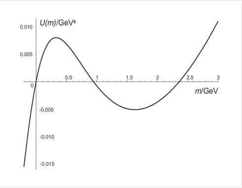
Figure 1: The effective potential $U(m)$ (see eq.(87)) for the parameter set given in the text as a function of the constituent quark mass $m$. All are given in dimensionless units.

5. Perturbative expansion of ${\cal Z}$

We shall restrict ourselves in this section to the perturbative treatment of the functional integral (19). The loop expansion will be considered in the next section.

5.1 The perturbative series

Let us devide the Lagrangian (20) in two parts. The free part, ${\cal L}_{0}$, is given by

$${\cal L}_{0}(R_{A})=\frac{G}{2}\,R_{A}^{2}+R_{A}(\Pi_{A}+\Delta_{A}).$$ (88)

The ’t Hooft interaction is considered as a perturbation ${\cal L}_{I}$

$${\cal L}_{I}(R_{A})=\frac{\kappa}{3!}\ \Phi_{ABC}R_{A}R_{B}R_{C}.$$ (89)

Thus the perturbative representation for the functional integral (19) can be written as

$${\cal Z}=N^{\prime}\,\exp\left(i\int\!{\cal L}_{I}(\hat{X}_{A})\right)\int\prod_{A}{\cal D}R_{A}\ e^{i\int\!{\cal L}_{0}(R_{A})}$$ (90)

where

$$\hat{X}_{A}=-i\,\frac{\delta}{\delta\Pi_{A}}\,.$$ (91)

Since the boson fields appear quadratically in eq.(90), they may be integrated out, yielding

$${\cal Z}=N\,\exp\left(i\int\!{\cal L}_{I}(\hat{X})\right)\exp\left(-i\int\frac{\bar{\Pi}_{A}^{2}}{2G}\right)$$ (92)

where $\bar{\Pi}_{A}=\Pi_{A}+\Delta_{A}$. The overall factor $N=(-2\pi i/G)^{9}N^{\prime}$ is unimportant in the following.

We want to calculate the effective action $\Gamma_{\mathrm{eff}}$, which by definition is the phase of ${\cal Z}$

$${\cal Z}=A(\bar{\Pi}_{A})\,\exp\left(i\int\!{\cal L}_{\mathrm{eff}}(\bar{\Pi}_{A})\right),$$ (93)

and $A(\bar{\Pi}_{A})$ is a real function. Comparing (92) and (93), one gets

$$\Gamma_{\mathrm{eff}}=i\ln\frac{A}{N}+\Gamma_{0}-i\ln\left(1+e^{-i\Gamma_{0}}\left(e^{i\int\!{\cal L}_{I}}-1\right)e^{i\Gamma_{0}}\right).$$ (94)

Here $\Gamma_{0}$ represents the leading order result for $\Gamma_{\mathrm{eff}}$

$$\Gamma_{0}=-\frac{1}{2G}\int\bar{\Pi}_{A}^{2}$$ (95)

while the second logarithm in eq.(94) is a source of $U_{\mathrm{A}}(1)$ breaking corrections which arise as a series in powers of the functional derivatives operator

$$\hat{\Gamma}_{I}=\int\!{\cal L}_{I}(\hat{X}_{A})=\frac{\kappa}{3!}\,\Phi_{ABC}\int\hat{X}_{A}\hat{X}_{B}\hat{X}_{C}\,.$$ (96)

To make this statement more explicit let us consider the expansion

$$\delta=e^{-i\Gamma_{0}}\left(e^{i\hat{\Gamma}_{I}}-1\right)e^{i\Gamma_{0}}=\sum_{m=1}^{\infty}\frac{i^{m}}{m!}\left(e^{-i\Gamma_{0}}\hat{\Gamma}_{I}e^{i\Gamma_{0}}\right)^{m}.$$ (97)

Taking into account the symmetry properties of the coefficients $\Phi_{ABC}$ and our previous result (18), we find

$$e^{-i\Gamma_{0}}\hat{\Gamma}_{I}e^{i\Gamma_{0}} \!\!\!=\!\!\! -\frac{\kappa}{3!}\,\Phi_{ABC}\int\left(\frac{1}{G^{3}}\,\bar{\Pi}_{A}\bar{\Pi}_{B}\bar{\Pi}_{C}-\frac{3}{G^{2}}\,\bar{\Pi}_{A}\bar{\Pi}_{B}\hat{X}_{C}\right.$$ (98)

$$\!\!\!+\!\!\! \left.\frac{3}{G}\,\bar{\Pi}_{A}\hat{X}_{B}\hat{X}_{C}-\hat{X}_{A}\hat{X}_{B}\hat{X}_{C}\right)$$

so that

$$\delta=\sum_{n=1}^{\infty}\kappa^{n}\delta_{n},$$ (99)

represents the effective action (94) as a perturbative series in powers of $\kappa$. For instance, up to and including the second order in $\kappa$ we have

$$\Gamma_{\mathrm{eff}}=i\ln\frac{A}{N}+\Gamma_{0}-i\kappa\delta_{1}-i\kappa^{2}\left(\delta_{2}-\frac{1}{2}\delta_{1}^{2}\right)-\ldots$$ (100)

where

$$\delta_{1}=\frac{-i}{3!G^{3}}\,\Phi_{ABC}\int\bar{\Pi}_{A}\bar{\Pi}_{B}\bar{\Pi}_{C}\,,$$ (101)

$$\delta_{2}-\frac{\delta^{2}_{1}}{2} \!\!\!=\!\!\! -\frac{i}{8G^{5}}\,\Phi_{ABC}\Phi_{AEF}\int\bar{\Pi}_{B}\bar{\Pi}_{C}\bar{\Pi}_{E}\bar{\Pi}_{F}$$ (102)

$$\!\!\!+\!\!\! \delta(0)\int\frac{\bar{\Pi}_{A}^{2}}{(8G^{2})^{2}}+[\delta(0)]^{2}\int\frac{3i}{32G^{3}}\,.$$

The real factor $A(\bar{\Pi})$ is always chosen such as to cancel the imaginary part of the effective action. To the approximation considered we have, for instance,

$$A(\bar{\Pi}) \!\!\!=\!\!\! N\,\exp\left\{\delta(0)\left(\frac{\kappa}{8G^{2}}\right)^{2}\int\bar{\Pi}_{A}^{2}\right\}$$ (103)

$$\!\!\!=\!\!\! N\left(1+\delta(0)\frac{\kappa^{2}}{64G^{4}}\int\bar{\Pi}_{A}^{2}+\ldots\right).$$

It contributes to the measure of the functional integral over $\sigma_{a},\phi_{a}$.

5.2 The problem with infinities

The terms with the $\delta(0)$ function require further explanation. The fact that auxiliary fields can lead to special problems with infinities is well-known [24]. For instance, a relevant case can be found in [25]: the new variable $\lambda$ is introduced in the photon self-energy diagram in a similar way, i.e., through the integral over a $\delta$-function, see eq.(8.18) of the book, which is equal to 1 and finally, after changes of variables in the whole expression eq.(8.19), the logarithmically divergent integral over $\lambda$ requires a cutoff.

A case involving a functional integral is given in [26] where the author considers as an example the non-linear $\sigma$-model and shows that the Gaussian functional integral with a field dependent coefficient in the exponent (there are no derivatives of fields there) leads to a $\delta(0)$ factor in the corresponding effective action (see also [27]).

In our case auxiliary variables have been introduced by eq.(4) and changing the order of integration in eq.(12) we finally came to a similar problem with infinities.

To see the origin of the encountered singularities in detail we shall use the language of Feynman diagrams. The graphs contributing to lowest order in $\kappa$ are shown in fig.2.

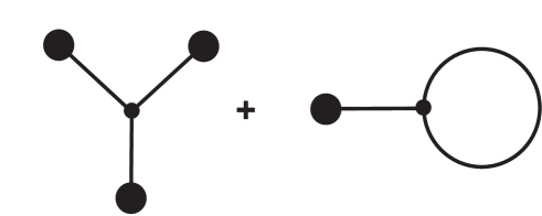
Figure 2: The lowest order graphs contributing to $\delta_{1}$.

In these diagrams, a line segment (straight or curved) stands for a “propagator”

$$\Delta_{AB}(x-y)=-(i/G)\delta_{AB}\delta(x-y),$$ (104)

extracted from the last exponent in eq.(92). A filled circle at one end of a line segment corresponds to the external field, $i\int\mathrm{d}^{4}x\bar{\Pi}_{A}(x)$, and a vertex joining three line segments is used for $i\kappa\Phi_{ABC}\int\mathrm{d}^{4}x$.

The first diagram represents the $\delta_{1}$ term in eq.(101). The contribution of the second tadpole diagram is equal to zero. Indeed, the vertex contains the group factor $\Phi_{ABC}$. The contraction of any two indices in this factor by $\delta_{AB}$ from the propagator (situation occuring for the tadpole graph) reduces it to zero, according to eq.(18). We thus find that tadpole diagrams do not contribute due to the flavor structure of the ’t Hooft interaction.

To next to leading order in $\kappa$ we have the four graphs shown in fig.3.

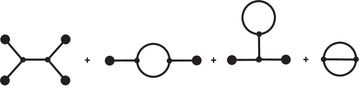
Figure 3: The diagrams of the $\kappa^{2}$ order contributing to $\delta_{2}$.

As we just learned, the third diagram does not contribute. The other ones correspond exactly to the three terms of eq.(102). The first tree diagram is finite. The second one-loop diagram has a divergent factor $\delta(0)$. The last two-loop diagram contributes as $\delta(0)^{2}$. These singularities were caused by the local structure of the last exponent in eq.(92) or, which is the same, by the $\delta(x-y)$ term in the propagator (104). We believe that if one would start from non-local NJL interactions, the singularities could be weaker or would even disappear.

The factor $\delta(0)$ requires a regularization. This is an expected trouble in the NJL model which is nonrenormalizable and, as a consequence, the fundamental interactions must be cut off. The cutoff is an effective, if crude, implementation of the known short distance behavior of QCD within the model. In the next subsection we shall discuss this procedure in the framework of the spectral method. The value of the cutoff can be fixed by confronting the model with the experiment. In this interpretation the model is effectively finite, including the higher order corrections.

The diagrams are a very convenient language to understand another feature related to the multi-loop contributions: the phase factor corresponding to the diagram can be simply calculated. Indeed, it is easy to see that for any diagram the formula

$$E=2I-3V$$ (105)

is fulfilled. Here $E$ is the number of external fields, $I$ stands for the number of internal lines, and $V$ is the number of vertices. On the other hand, the number of loops, $L$, is given by

$$L=I-V-E+1\,.$$ (106)

This is because the number of loops in a diagram is equal to the number of $\delta$ functions surviving after all integrations over coordinates are performed, exept for one over-all integration related to the effective action. Every internal line contributes one $\delta$ function, but every vertex or external field carries an integration over the corresponding coordinate, and thus reduces the number of $\delta$ functions by one.

This result shows that the overall phase factor of a given graph $i^{I-E-V}=i^{L-1}$ is entirely determined by the number of loops. In particular, diagrams with an even number of loops contribute to the effective action (the argument of ${\cal Z}$), while the diagrams with odd number of loops contribute to the measure (the modulus of ${\cal Z}$), see eq.(93).

5.3 The spectral representation method

The problem with $\delta(0)$ singularities can be analysed with more accurate methods. In this subsection we shall use the spectral representation method to evaluate the integral (15).

Let us consider, for simplicity, a one-dimensional field theory approximation for the integral (15). The number of dimensions does not matter here. The extension to the real case is straightforward. We also put our system in an interval of size $L$, i.e. $-L/2\leq x\leq L/2$, assuming the limit $L\to\infty$ in the end of calculations. The Fourier decomposition of the fields $f_{a}(x)=\{s_{a},p_{a},\sigma_{a},\phi_{a}\}$ inside the interval is

$$f_{a}(x)=\sum_{n=-\infty}^{+\infty}f_{n}^{a}\,\exp\left(i2\pi\frac{nx}{L}\right).$$ (107)

This corresponds to the periodic boundary conditions $f_{a}(-L/2)=f_{a}(L/2)$. The Fourier coefficients $f_{n}^{a}$ represent the field $f_{a}(x)$ inside the considered interval

$$f_{n}^{a}=\frac{1}{L}\int_{-L/2}^{+L/2}\mathrm{d}x\,f_{a}(x)\exp\left(-i2\pi\frac{nx}{L}\right),\qquad f_{-n}=f^{*}_{n}.$$ (108)

Then we have

$$\int\mathrm{d}x\,{\cal L}(x)\simeq\int_{-L/2}^{L/2}\mathrm{d}x\,{\cal L}(x)=L{\cal L}\,,$$ (109)

where ${\cal L}$ is devided in two parts: the free one ${\cal L}_{0}$, and the perturbation ${\cal L}_{I}$

$${\cal L}_{0}=\sum_{n=-\infty}^{+\infty}\left[\frac{G}{2}\left(s^{a}_{n}s^{a}_{-n}+p^{a}_{n}p^{a}_{-n}\right)+\sigma^{a}_{n}s^{a}_{-n}+\phi^{a}_{n}p^{a}_{-n}\right],$$ (110)

$${\cal L}_{I}=\frac{\kappa}{32}A_{abc}\sum_{n,m,k}s^{a}_{n}\left(s^{b}_{m}s^{c}_{k}-3p^{b}_{m}p^{c}_{k}\right)\delta_{n+m+k,0}.$$ (111)

The functional integral can be understood as the product of integrals over the Fourier coefficients

$$\int\limits_{-\infty}^{+\infty}{\cal D}s_{a}(x){\cal D}p_{a}(x)\to\prod_{n}\int\limits_{-\infty}^{+\infty}\mathrm{d}s_{n}^{a}\mathrm{d}p_{n}^{a}$$ (112)

and in the perturbative approximation can be written as

$${\cal Z}[\sigma,\phi]\sim\exp\left\{iL\hat{\cal L}_{I}(S_{n}^{a},P_{n}^{a})\right\}\prod_{n}\int\limits_{-\infty}^{+\infty}\mathrm{d}s_{n}^{a}\mathrm{d}p_{n}^{a}\exp\left(iL{\cal L}_{0}\right)$$ (113)

where

$$S^{a}_{n}=-\frac{i}{L}\frac{\partial}{\partial\sigma^{a}_{-n}}\,,\qquad P^{a}_{n}=-\frac{i}{L}\frac{\partial}{\partial\phi^{a}_{-n}}\,.$$ (114)

It is convenient to use the normalized functional ${\cal Z}$ defined as

$${\cal Z}=\frac{{\cal Z}[\sigma,\phi]}{{\cal Z}[0,0]}\,.$$ (115)

The Gaussian functional integrals can be simply evaluated, for instance, one has

$$I[\sigma] \!\!\!=\!\!\! \prod_{n}\int\limits_{-\infty}^{+\infty}\mathrm{d}s_{n}\,\exp\left\{iL\sum_{n=-\infty}^{+\infty}\left(\frac{G}{2}s_{n}s_{-n}+\sigma_{n}s_{-n}\right)\right\}$$ (116)

$$\!\!\!=\!\!\! \int\limits_{-\infty}^{+\infty}\mathrm{d}s_{0}\,\exp\left\{iL\left(\frac{G}{2}s_{0}^{2}+\sigma_{0}s_{0}\right)\right\}$$

$$\!\!\!\times\!\!\! \prod_{l=1}^{\infty}\int\limits_{-\infty}^{+\infty}\mathrm{d}s_{l}\mathrm{d}s^{*}_{l}\,\exp\left\{iL\sum_{l=1}^{+\infty}\left(Gs_{l}s^{*}_{l}+\sigma_{l}s^{*}_{l}+\sigma^{*}_{l}s_{l}\right)\right\}$$

$$\!\!\!=\!\!\! I[0]\exp\left\{-\frac{iL}{2G}\sum_{n=-\infty}^{+\infty}\sigma_{n}\sigma_{-n}\right\}.$$

Thus the functional integration yields

$${\cal Z}\sim\exp\left\{iL\hat{\cal L}_{I}(S_{n}^{a},P_{n}^{a})\right\}\exp\left\{-\frac{iL}{2G}\sum_{n=-\infty}^{+\infty}\left(\sigma_{n}\sigma_{-n}+\phi_{n}\phi_{-n}\right)\right\}.$$ (117)

We should now calculate partial derivatives to obtain the effective action $\Gamma_{eff}$

$${\cal Z}\sim A[\sigma,\phi]\,e^{i\Gamma_{eff}}.$$ (118)

As before (see subsection 3.2) we have

$$\Gamma_{eff}=i\ln A[\sigma,\phi]+\Gamma_{0}-i\ln\left(1+e^{-i\Gamma_{0}}\left(e^{i\hat{\Gamma}_{I}}-1\right)e^{i\Gamma_{0}}\right),$$ (119)

where $A[\sigma,\phi]$ is fixed by the requirement that the effective action $\Gamma_{eff}$ is real. Here $\Gamma_{0}$ represents the leading order action

$$\Gamma_{0}=-\frac{L}{2G}\sum_{n=-\infty}^{\infty}\left(\sigma^{a}_{n}\sigma^{a}_{-n}+\phi^{a}_{n}\phi^{a}_{-n}\right).$$ (120)

The logarithm in eq.(119) is a source of $U_{\mathrm{A}}(1)$ breaking corrections which arise as a series in powers of the partial derivatives

$$\hat{\Gamma}_{I} \!\!\!=\!\!\! L{\cal L}_{I}(S^{a}_{n},P^{a}_{n})$$ (121)

$$\!\!\!=\!\!\! \frac{\kappa L}{32}A_{abc}\sum_{n,m,k}S^{a}_{n}\left(S^{b}_{m}S^{c}_{k}-3P^{b}_{m}P^{c}_{k}\right)\delta_{n+m+k,0}\,.$$

One has the following result

$$e^{-i\Gamma_{0}}\hat{\Gamma}_{I}e^{i\Gamma_{0}} \!\!\!=\!\!\! -\frac{\kappa L}{32}\,A_{abc}\sum_{n,m,k}\delta_{n+m+k,0}\left[\frac{1}{G^{3}}\,\sigma^{a}_{n}(\sigma^{b}_{m}\sigma^{c}_{k}-3\phi^{b}_{m}\phi^{c}_{k})\right.$$ (122)

$$\!\!\!-\!\!\! \frac{3}{G^{2}}\,(\sigma^{b}_{m}\sigma^{c}_{k}-\phi^{b}_{m}\phi^{c}_{k})S^{a}_{n}+\frac{6}{G^{2}}\,\sigma^{a}_{n}\phi^{b}_{m}P^{c}_{k}$$

$$\!\!\!+\!\!\! \frac{3}{G}\,\sigma^{a}_{n}(S^{b}_{m}S^{c}_{k}-P^{b}_{m}P^{c}_{k})-\frac{6}{G}\,\phi^{a}_{n}S^{b}_{m}P^{c}_{k}$$

$$\!\!\!-\!\!\! \left.S^{a}_{n}(S^{b}_{m}S^{c}_{k}-3P^{b}_{m}P^{c}_{k})\right].$$

Therefore, expanding

$$\delta=e^{-i\Gamma_{0}}\left(e^{i\hat{\Gamma}_{I}}-1\right)e^{i\Gamma_{0}}=\sum_{n=1}^{\infty}\kappa^{n}\delta_{n},$$ (123)

one can determine

$$\delta_{1}=\frac{-iL}{32G^{3}}\,A_{abc}\sum_{n,m,k}\sigma^{a}_{n}(\sigma^{b}_{m}\sigma^{c}_{k}-3\phi^{b}_{m}\phi^{c}_{k})\delta_{n+m+k,0}\,,$$ (124)

$$\delta_{2} \!\!\!=\!\!\! \frac{\delta^{2}_{1}}{2}-i\,\frac{9L}{64(2G)^{5}}\,A_{abc}A_{a\bar{b}\bar{c}}\sum_{m,k,\bar{m},\bar{k}}\delta_{m+k+\bar{m}+\bar{k},0}\left[\,4\sigma^{b}_{m}\sigma^{\bar{b}}_{\bar{m}}\phi^{c}_{k}\phi^{\bar{c}}_{\bar{k}}\right.$$ (125)

$$\!\!\!+\!\!\! \left.\left(\sigma^{b}_{m}\sigma^{c}_{k}-\phi^{b}_{m}\phi^{c}_{k}\right)\left(\sigma^{\bar{b}}_{\bar{m}}\sigma^{\bar{c}}_{\bar{k}}-\phi^{\bar{b}}_{\bar{m}}\phi^{\bar{c}}_{\bar{k}}\right)\,\right]$$

$$\!\!\!+\!\!\! \frac{1}{(8G^{2})^{2}}\sum_{n}\left(\sigma^{a}_{n}\sigma^{a}_{-n}+\phi^{a}_{n}\phi^{a}_{-n}\right)\sum_{m}1+\frac{3i}{32LG^{3}}\left(\sum_{m}1\right)^{2}\,,$$

and so forth.

The effective action can be also expanded in $\kappa$

$$\Gamma_{eff}=i\ln A[\sigma,\phi]+\Gamma_{0}-i\kappa\delta_{1}-i\kappa^{2}\left(\delta_{2}-\frac{\delta_{1}^{2}}{2}\right)+{\cal O}(\kappa^{3}),$$ (126)

where one assumes that $\ln A[\sigma,\phi]$ must be also expanded, i.e.,

$$A[\sigma,\phi] \!\!\!=\!\!\! 1+\kappa\beta_{1}+\kappa^{2}\beta_{2}+{\cal O}(\kappa^{3}),$$

$$\ln A[\sigma,\phi] \!\!\!=\!\!\! \kappa\beta_{1}+\kappa^{2}\left(\beta_{2}-\frac{\beta_{1}^{2}}{2}\right)+{\cal O}(\kappa^{3}),$$ (127)

and, up to the considered order in $\kappa$, we have

$$\beta_{1}=0,\qquad\beta_{2}=\frac{1}{(8G^{2})^{2}}\sum_{n}\left(\sigma^{a}_{n}\sigma^{a}_{-n}+\phi^{a}_{n}\phi^{a}_{-n}\right)\sum_{m}1\,.$$ (128)

Therefore the perturbative action systematically obtains $U_{\mathrm{A}}(1)$ breaking corrections in $\kappa^{n}$, which we collect in the corresponding part of the action, $\Gamma_{n}$,

$$\Gamma_{eff}=\sum_{n=0}^{+\infty}\Gamma_{n}\,,$$ (129)

where $\Gamma_{0}$ is given by eq.(120), and

$$\Gamma_{1} \!\!\!=\!\!\! -\frac{\kappa L}{32G^{3}}\,A_{abc}\sum_{n,m,k}\sigma^{a}_{n}(\sigma^{b}_{m}\sigma^{c}_{k}-3\phi^{b}_{m}\phi^{c}_{k})\delta_{n+m+k,0}\,,$$

$$\Gamma_{2} \!\!\!=\!\!\! -\frac{9\kappa^{2}L}{64(2G)^{5}}\,A_{abc}A_{a\bar{b}\bar{c}}\sum_{m,k,\bar{m},\bar{k}}\delta_{m+k+\bar{m}+\bar{k},0}\left[\,4\sigma^{b}_{m}\sigma^{\bar{b}}_{\bar{m}}\phi^{c}_{k}\phi^{\bar{c}}_{\bar{k}}\right.$$ (130)

$$\!\!\!+\!\!\! \left.\left(\sigma^{b}_{m}\sigma^{c}_{k}-\phi^{b}_{m}\phi^{c}_{k}\right)\left(\sigma^{\bar{b}}_{\bar{m}}\sigma^{\bar{c}}_{\bar{k}}-\phi^{\bar{b}}_{\bar{m}}\phi^{\bar{c}}_{\bar{k}}\right)\,\right].$$

Here an unessential constant (for the physical action) has been omitted in $\Gamma_{2}$.

Using the well known relation

$$\sum_{n=-\infty}^{+\infty}\exp\left(i\frac{2\pi x}{L}n\right)=L\sum_{n=-\infty}^{\infty}\delta(x-Ln)=L\delta(x)$$ (131)

where on the last step we used the fact that in the problem considered all $x$-dependent functions are integrated only in the interval $-L/2\leq x\leq L/2$ and, therefore, only the term with $n=0$ can contribute, one can obtain that

$$\sum_{n}f^{a}_{n}f^{b}_{k-n}=\frac{1}{L}\int_{-L/2}^{L/2}\mathrm{d}x\,f_{a}(x)f_{b}(x)\exp(-i2\pi kx/L).$$ (132)

As a result, taking the infinite-volume limit $L\to\infty$, we have, for instance,

$$\Gamma_{0}=-\frac{1}{2G}\int\limits_{-\infty}^{+\infty}\mathrm{d}x\,\left(\sigma^{2}_{a}(x)+\phi^{2}_{a}(x)\right)\,.$$ (133)

Using the following relation

$$\sum_{n_{1},n_{2},\ldots,n_{i}}\!\!\!f^{a_{1}}_{n_{1}}f^{a_{2}}_{n_{2}}\ldots f^{a_{i}}_{n_{i}}\,\delta_{n_{1}+n_{2}+\ldots+n_{i},0}=\frac{1}{L}\int_{-L/2}^{L/2}\!\mathrm{d}x\,f^{a_{1}}(x)f^{a_{2}}(x)\ldots f^{a_{i}}(x)$$ (134)

in (5.3 The spectral representation method), and taking the limit $L\to\infty$ one finds that

$$\Gamma_{1} \!\!\!=\!\!\! -\frac{\kappa}{32G^{3}}\,A_{abc}\int\limits_{-\infty}^{+\infty}\!\mathrm{d}x\,\sigma_{a}(x)\left[\sigma_{b}(x)\sigma_{c}(x)-3\phi_{b}(x)\phi_{c}(x)\right],$$

$$\Gamma_{2} \!\!\!=\!\!\! -\frac{9\kappa^{2}}{64(2G)^{5}}\,A_{abc}A_{a\bar{b}\bar{c}}\int\limits_{-\infty}^{+\infty}\!\mathrm{d}x\,\left[\,4\sigma_{b}(x)\sigma_{\bar{b}}(x)\phi_{c}(x)\phi_{\bar{c}}(x)\right.$$ (135)

$$\!\!\!+\!\!\! \left.\left(\sigma_{b}(x)\sigma_{c}(x)-\phi_{b}(x)\phi_{c}(x)\right)\left(\sigma_{\bar{b}}(x)\sigma_{\bar{c}}(x)-\phi_{\bar{b}}(x)\phi_{\bar{c}}(x)\right)\,\right].$$

The infinite-volume limit for the expansion coefficient $\beta_{2}$ needs additional explanation. Here one should define carefully the limiting procedure. We have

$$\beta_{2}=\frac{1}{(8G^{2})^{2}}\int_{-L/2}^{L/2}\!\mathrm{d}x\,\left(\sigma_{a}(x)\sigma_{a}(x)+\phi_{a}(x)\phi_{a}(x)\right)\frac{1}{L}\sum_{m=-\infty}^{+\infty}1\,.$$ (136)

The integral has a smooth $L\rightarrow\infty$ limit, but contains the local factor, which can be understood as a $\delta$-function singularity, $\delta(0)$. It is clear from eq.(131) that the infinite value

$$\frac{1}{L}\sum_{n=-\infty}^{+\infty}1=\delta(0)$$ (137)

appears as a common factor on the right hand side of eq.(136), representing the density of the Fourier harmonics in the interval. It must be regularized by cutting an upper part of the spectrum, e.g.,

$$\delta(0)_{\mbox{\footnotesize reg}}=\frac{1}{L}\sum_{n=-N}^{N}1=\frac{2N+1}{L}$$ (138)

where $N$ is large enough. Let us recall that the limit $L\to\infty$ is to be taken afterwards. Therefore one should clarify the meaning of $N$ being large. There are two possibilities. One can fix $N\gg 1$ without any relation to the size of the box. In this case, in the limit $L\to\infty$, the $\delta$-function vanishes. Alternatively, one can relate $N$ with $L$ by introducing a momentum space cutoff $\Lambda$: $N(L)=L\Lambda/(4\pi)\gg 1$. Unlike $L$ the cutoff $\Lambda$ has an obvious physical meaning giving the scale of momenta relevant for the problem. Indeed, the $n$th harmonic has a momentum $p_{n}=2\pi n/L$. The size of the considered box is the difference $p_{N}-p_{-N}=4\pi N/L=\Lambda$. The scale cannot be eliminated by taking the limit $L\to\infty$. One has instead

$$\delta(0)_{\mbox{\footnotesize reg}}=\frac{\Lambda}{2\pi}+\frac{1}{L}\,,$$ (139)

where only the second term does not contribute in the limit $L\rightarrow\infty$. By introducing the cutoff $\Lambda$, we suppose that the density of Fourier harmonics has a finite value which can be fixed phenomenologically. This is the scenario which we will favor in the following.

6. The loop expansion of ${\cal Z}$

The perturbative series, considered in the previous section, can be resummed: first summing all diagrams with no closed loops (tree graphs), then those with one closed loop, etc. As we have already discussed, this can be done by generalizing the method of subsec.3.6. The tree graphs have been summed in this way in [15], and the one-loop graphs in [21]. The two-loop approximation is the next to lowest order result which contributes to the effective action, since the one-loop diagrams contribute solely to the amplitude.

6.1 The two-loop approximation

In this subsection we present a detailed computation of the two-loop approximation to the effective mesonic action generated by the functional

$${\cal Z}[\Pi,\Delta] \!\!\!\sim\!\!\! {\cal N}\exp\left(i\int\mathrm{d}^{4}x{\cal L}_{\mathrm{st}}^{(i=1)}\right)$$ (140)

$$\!\!\!\times\!\!\! \int\limits^{+\infty}_{-\infty}\prod_{A}{\cal D}\bar{R}_{A}\ \exp\left(\frac{i}{2}\int\mathrm{d}^{4}x{\cal L}_{AB}^{\prime\prime}({\cal R}^{(i=1)})\bar{R}_{A}\bar{R}_{B}\right)$$

$$\!\!\!\times\!\!\! \sum_{n=0}^{\infty}\frac{1}{n!}\left(i\frac{\kappa}{3!}\ \Phi_{ABC}\int\mathrm{d}^{4}x\bar{R}_{A}\bar{R}_{B}\bar{R}_{C}\right)^{n}\qquad$$

Note that in comparison with eq.(82), only one critical point, related to the stable configuration, must be considered. It is the solution with $i=1$ in eqs.(81). We shall identify ${\cal L}_{\mathrm{st}}^{(i=1)}={\cal L}_{\mathrm{st}}$, and ${\cal L}_{AB}^{\prime\prime}({\cal R}^{(i=1)})={\cal L}_{AB}^{\prime\prime}$ in the following.

By replacing the continuum of spacetime positions with a discrete lattice of points surrounded by separate regions of small spacetime volume $\Omega$, the functional integral (140) may be reexpressed as a Gaussian multiple integral over a finite number of real variables $R_{A}(x)$ for a fixed spacetime point $x$. We think of ${\cal D}R_{A}$ as the infinite product ${\cal D}R_{A}\to\prod_{x}\mathrm{d}R_{A}(x)$, $\int\mathrm{d}^{4}x\to\Omega\sum_{x}$.

$${\cal Z}[\Pi,\Delta] \!\!\!\sim\!\!\! {\cal N}\prod_{x}\left\{\,\exp\left(i\Omega{\cal L}_{\mathrm{st}}\right)\int\limits^{+\infty}_{-\infty}\prod_{A}\mathrm{d}\bar{R}_{A}\,\exp\left(\frac{i}{2}\Omega{\cal L}_{AB}^{\prime\prime}\bar{R}_{A}\bar{R}_{B}\right)\right.$$ (141)

$$\!\!\!\times\!\!\! \left.\!\!\left(1-\frac{(\kappa\Omega)^{2}}{2!(3!)^{2}}\Phi_{ABC}\Phi_{DEF}\bar{R}_{A}\bar{R}_{B}\bar{R}_{C}\bar{R}_{D}\bar{R}_{E}\bar{R}_{F}+\ldots\right)\right\}.$$

The last sum contains only terms with even powers of $\bar{R}_{A}$, the odd powers do not contribute under the Gaussian integration. The dots mean the terms corresponding to the three-loop contribution and higher.

Let us do the Gaussian integrals

$${\cal Z}[\Pi,\Delta]\sim{\cal N}\prod_{x}\left\{\,I_{0}\,\exp\left(i\Omega{\cal L}_{\mathrm{st}}\right)\left(1+i\frac{\kappa^{2}\Phi_{ABC}\Phi_{DEF}\delta_{ABCDEF}}{72\Omega N(N+2)(N+4)}{\cal M}+\ldots\right)\right\}.\\$$

Here

$${\cal M}=\left(\mbox{tr}\left.{\cal L}^{\prime\prime}\right.^{-1}\right)^{3}\!+6\,\mbox{tr}\left.{\cal L}^{\prime\prime}\right.^{-1}\mbox{tr}(\left.{\cal L}^{\prime\prime}\right.^{-1})^{2}\!+8\,\mbox{tr}\left(\left.{\cal L}^{\prime\prime}\right.^{-1}\right)^{3},$$ (142)

and $I_{0}$ is a one-loop contribution

$$I_{0}=\frac{1}{\sqrt{\det{\cal L}^{\prime\prime}}}\left(\frac{2\pi}{\Omega}\right)^{\frac{N}{2}}\exp\left(i\frac{\pi}{4}\sum\limits_{j=1}^{N}\mbox{sgn}(\lambda_{j})\right)$$ (143)

where $\lambda_{j}$ are eigenvalues of the $N\times N$ matrix ${\cal L}^{\prime\prime}_{AB}$. In our case $N=18$. $\left.{\cal L}^{\prime\prime}\right.^{-1}$ is an inverse matrix of ${\cal L}^{\prime\prime}$. The totally symmetric symbol $\delta_{ABCDEF}$ generalizes an ordinary Kronecker delta symbol $\delta_{AB}$ by the recurrent relation

$$\delta_{ABCDEF}=\delta_{AB}\delta_{CDEF}+\delta_{AC}\delta_{BDEF}+\ldots+\delta_{AF}\delta_{BCDE}\,.$$ (144)

One can find that

$$\Phi_{ABC}\Phi_{DEF}\delta_{ABCDEF}=6\Phi_{ABC}\Phi_{ABC}=\frac{27}{4}\,.$$ (145)

Up to the given accuracy we have in eq.(6.1 The two-loop approximation)

$$\prod_{x}\left(\,I_{0}\,e^{i\Omega{\cal L}_{\mathrm{st}}}\left(1+iF\right)\right)=\prod_{x}\left(\,I_{0}\,e^{i(\Omega{\cal L}_{\mathrm{st}}+F)}\right)$$

$$=\left(\prod_{x}I_{0}\right)\left(\prod_{x}e^{i(\Omega{\cal L}_{\mathrm{st}}+F)}\right)=\left(\prod_{x}I_{0}\right)e^{i\Omega\sum_{x}({\cal L}_{\mathrm{st}}+F/\Omega)}$$ (146)

It shows that in the continuum limit the two-loop correction contributes to the effective Lagrangian as

$${\cal L}_{\mathrm{eff}}={\cal L}_{\mathrm{st}}+\frac{3\kappa^{2}[\delta(0)]^{2}{\cal M}}{32N(N+2)(N+4)}\,.$$ (147)

This is our final expression for the effective Lagrangian in the two-loop approximation.

Let us do some estimates to justify the result. For this purpose let us simplify the integral (140). After neglecting the symmetry group and discretizing the spacetime it takes the form

$${\cal Z}[\Pi,\Delta]\sim\prod_{x}\int\mathrm{d}R_{x}\exp\left\{i\Omega\left({\cal L}_{\mathrm{st}}+\frac{1}{2}{\cal L}_{\mathrm{st}}^{\prime\prime}R_{x}^{2}+\frac{1}{3!}{\cal L}_{\mathrm{st}}^{\prime\prime\prime}R_{x}^{3}\right)\right\}\,.$$ (148)

To justify the stationary phase approximation for the integral (148) we assume that

$$\Omega{\cal L}_{\mathrm{st}}\gg 1.$$ (149)

The dominating role of the Gaussian integral is reflected in the fact that essential values for $R_{x}$ in the integral have the order $R_{x}^{2}\sim 1/(\Omega{\cal L}_{\mathrm{st}}^{\prime\prime})$. For the cubic term it follows then

$$\Omega{\cal L}_{\mathrm{st}}^{\prime\prime\prime}R_{x}^{3}\sim\sqrt{\frac{({\cal L}_{\mathrm{st}}^{\prime\prime\prime})^{2}}{\Omega({\cal L}_{\mathrm{st}}^{\prime\prime})^{3}}}\sim\sqrt{\frac{\kappa^{2}}{\Omega G^{3}}}\sim\sqrt{\zeta}\ ,$$ (150)

where we have used that in the model considered here, ${\cal L}_{\mathrm{st}}^{\prime\prime\prime}\sim\kappa$, ${\cal L}_{\mathrm{st}}^{\prime\prime}\sim G$. If the parameters of the model can be chosen in such a way that the inequality $\zeta\ll 1$ is fulfilled, the cubic power of $R_{x}$ yields terms that go to zero relative to the Gaussian term as $\zeta\to 0$, and the stationary phase approximation will be justified. Note that $\Omega$ may be written as an ultraviolet divergent integral regularized by introducing a cutoff $\Lambda$

$$\Omega^{-1}=\delta^{4}(0)\sim\int_{-\Lambda/2}^{\Lambda/2}\frac{\mathrm{d}^{4}k_{\mathrm{E}}}{(2\pi)^{4}}=\left(\frac{\Lambda}{2\pi}\right)^{4}.$$ (151)

Therefore, the inequality restrics the value of $\Lambda$ from above.

Meanwhile, it is interesting to see that the inequality $\zeta\ll 1$ is an exact equivalent of (149). Indeed, in the essential region, i.e., around a sharp minimum, one has ${\cal L}_{\mathrm{st}}^{\prime}\sim R_{x}{\cal L}_{\mathrm{st}}$, ${\cal L}_{\mathrm{st}}^{\prime\prime}\sim R_{x}^{2}{\cal L}_{\mathrm{st}}$, and so on, thus

$$\zeta\sim\frac{({\cal L}_{\mathrm{st}}^{\prime\prime\prime})^{2}}{\Omega({\cal L}_{\mathrm{st}}^{\prime\prime})^{3}}\sim\frac{({R_{x}^{3}\cal L}_{\mathrm{st}})^{2}}{\Omega(R_{x}^{2}{\cal L}_{\mathrm{st}})^{3}}\sim\frac{1}{\Omega{\cal L}_{\mathrm{st}}}\ .$$ (152)

To summarize, the asymptotical series (141) with the ultraviolet cutoff imposed is sensible. One deals here, actually, with a series in powers of the dimensionless parameter $\zeta$. The expansion is formally justified for $\zeta\ll 1$.

6.2 Some final comments

Several comments are in order:

(1) We believe that it is the first time that loop corrections to the effective action have been obtained at next to lowest order in the bosonization procedure.

(2) This is a nonrenormalizable theory; so we should expect an explicit dependence on the cutoff in the result. This is indeed the case: the $[\delta(0)]^{2}$ factor is understood as an effective arbitrary parameter $(\Lambda/(2\pi))^{8}$ which together with the other coupling constants of the model, $G$ and $\kappa$, forms a dimensionless expansion parameter $\zeta\sim\kappa^{2}\Lambda^{4}/G^{3}$, the latter must be small to justify the loop expansion. This requirement restricts the value of $\Lambda$ from above.

(3) The field-dependent factor ${\cal M}$ contains all possible mesonic vertices, including the $\sigma$-tadpole contribution to the gap equation, and contributions to the masses of scalar and pseudoscalar nonets. These contributions might be interesting and worth studying phenomenologically.

(4) Without future phenomenological considerations it is difficult to say at this stage if the loop expansion is a better approximation scheme than the ordinary perturbative theory considered above. It is certainly not worse if $\kappa$ is small, since the set of graphs with $2n$ loops includes, as a subset, all graphs of $\kappa^{n+1}$th order or higher in the coupling constant. Thus, in the tree approximation the term $\sim\kappa$ will dominate, the two-loop result will include the $\kappa$ and $\kappa^{2}$ order contributions completely, and so on. On the other hand, if perturbative corrections are sufficiently large, the loop expansion can be more appropriate.

(5) We believe that techniques developed here to obtain the two-loop contribution can be easily applied to higher orders in the loop expansion. We also hope that some of our findings can be used in more advanced calculations with non-local effective quark Lagrangians.

7. Summary and outlook

The purpose of this paper has been to consider several mathematical aspects which are related with the $U_{\mathrm{A}}(1)$ axial symmetry breaking by the ’t Hooft determinant within the framework of the NJL model. Among them is the question related to the stability of the ground state, the relevance of an hierarchy in multi-quark interactions, and the development of techniques for studying the effective Lagrangian beyond lowest order in $U_{\mathrm{A}}(1)$ breaking effects, so that quark – anti-quark bound-state phenomena can be examined in detail.

We have shown that in this picture there is an apparent problem: the model has no ground state. This conclusion is based on the stationary phase method applied to the generating functional of the model. This approach is a well established technique which allows to identify straightforwardly all critical points, i.e., all solutions ${\cal R}_{A}^{(i)}$ of the stationary phase equations associated with the auxiliary bosonic variables, and obtain finally the gap equations which are the local extrema conditions for the corresponding effective potential. It has been shown that these gap equations have no phenomenologically acceptable solutions at leading order of the stationary phase approach.

If the theory has no ground state, the theory is useless for phenomenology. This fact, however, can be used to obtain some constraints with a clear phenomenological content. Indeed, let us assume for a moment that the ’t Hooft coupling $\kappa$ scales as $N_{c}^{1-N_{f}}$. It would mean that the Lagrangian density ${\cal L}_{\mathrm{H}}$ scales with $N_{c}$, being comparable to ${\cal L}_{\mathrm{NJL}}$. We already know that such theory has no ground state and must be rejected, thus this counting for $\kappa$ is not acceptable. Indeed, all phenomenological facts related with the known solution of the $U_{\mathrm{A}}(1)$ problem provide for abundant evidence in favour of a different large $N_{c}$ identification: $\kappa\sim 1/N_{c}^{N_{f}}$.

There are several alternatives to save the situation. We have considered here the way based on the perturbative treatment of the multi-quark system. Two new results have been obtaind in Sec.3 in this connection:

(1) We have shown that the perturbative approach is related to a one critical point result of the stationary phase calculations: both represent the same function, giving different series developments for it.

(2) We have shown that this function, if one would find it, is not equal to the starting integral (21), and is also not an asymptotical series of it.

Both these findings are new to our knowledge and serve to understand better the approximations used. They probably cannot be rigorously proven for the functional case, but definitely solve the problem in the following way: by removing the destructive effect of the singular critical point in the generating functional, the system can be treated perturbatively around the stable ground state of the NJL model. Therefore, this is a reasonable step for qualitative phenomenological considerations at least.

Two series expansions have been discussed in this context. We have calculated the first order corrections to both of them and gave the complete classification of the terms of the series, separating contributions to the effective meson Lagrangian from the ones to the measure. We have shown that loop corrections serve to obtain approximately (i.e., in the framework of the local model which has been considered here) the less divergent or even finite contributions which would originate within a more refined consideration with non-local multi-quark vertices.

The new corrections, on which we report, are the direct consequence of the ’t Hooft term in the Lagrangian and in this sense they are interesting by themselves and will survive even if theory and experiment disagree. Were this the case, it would only mean that some essential details in the multi-quark effective Lagrangian are still missing, thus stimulating work in this direction. In the opposite case, if the predictions are close to the data, our findings would put the model on firmer grounds.

Another commonly used technique is the mean-field method [16]. It is easy to see that the gap equations that one gets within this approach are equivalent to the ones of the stationary phase method, when the latter is considered at leading order and the contribution of the singular critical point is omitted. Therefore, the effective potentials coincide in this case. It is clear from this comparison that the loop corrections found in our work can be also considered as a step beyond the leading order mean-field result.

There is another way, which yields a rigorous mathematical solution of the ground state problem above: one can take into account the eight-quark or higher order interactions with hope to stabilize the vacuum. This approach will be considered elsewhere [28].

Appendix

The Airy function

The Airy function $Ai(x)$ is defined as

$$Ai(x)=\frac{1}{2\pi}\int\limits_{-\infty}^{+\infty}\!\mathrm{d}t\,\exp\left(i\left(\frac{t^{3}}{3}+xt\right)\right)\,,$$ (153)

at real values of $x$ and can be analytically continued to the whole complex plane $x\to z$ as an entire function of $z$.
(a) It is real, if $z$ is real.
(b) It decreases exponentially for $|\mbox{arg}\,z|<\pi/3$.
(c) It increases exponentially for $\pi/3<\mbox{arg}\,z<\pi$, and $-\pi<\mbox{arg}\,z<-\pi/3$.
(d) It oscillates at $\mbox{arg}\,z=\pm\pi/3,\pi$.
(e) On the real axis the function has the following asymptotics

$$Ai(x)\sim\frac{x^{-1/4}}{2\sqrt{\pi}}\exp\left(-\frac{2}{3}x^{3/2}\right)\qquad(x\to+\infty).$$ (154)

$$Ai(x)\sim\frac{(-x)^{-1/4}}{\sqrt{\pi}}\left[\cos\left(\frac{2}{3}(-x)^{3/2}-\frac{\pi}{4}\right)+{\cal O}(x^{-3/2})\right]\qquad(x\to-\infty).$$ (155)

References

• [1] S. Weinberg, Physica A96 (1979) 327.
• [2] J. Gasser and H. Leutwyler, Ann. of Phys. (N.Y.) 158 (1984) 142; J. Gasser and H. Leutwyler, Nucl. Phys. B250 (1985) 465.
• [3] see, for instance, recent reviews: D. Diakonov, Progr. in Part. and Nucl. Phys. 51 (2003) 173, hep-ph/0212026; E. V. Shuryak, Phys. Reports 391 (2004) 381.
• [4] G. ’t Hooft, Phys. Rev. D14 (1976) 3432; Erratum: ibid D18 (1978) 2199.
• [5] Yu. A. Simonov, Phys. Lett. B412 (1997) 371, hep-th/9703205.
• [6] G. S. Bali, Phys. Rept. 343 (2001) 1, hep-ph/0001312.
• [7] Yu. A. Simonov, Phys. Rev. D65 (2002) 094018, hep-ph/0201170.
• [8] Y. Nambu and G. Jona-Lasinio, Phys. Rev. 122 (1961) 345; 124 (1961) 246; V. G. Vaks and A. I. Larkin, Zh. Γ‰ksp. Teor. Fiz. 40 (1961) 282.
• [9] T. Eguchi, Phys. Rev. D14 (1976) 2755; K. Kikkawa, Progr. Theor. Phys. 56 (1976) 947.
• [10] M. K. Volkov and D. Ebert, Sov. J. Nucl. Phys. 36 (1982) 736; D. Ebert and M. K. Volkov Z. Phys. C16 (1983) 205.
• [11] M. K. Volkov, Ann. Phys. (N.Y.) 157 (1984) 282; A. Dhar and S. Wadia, Phys. Rev. Lett. 52 (1984) 959; A. Dhar, R. Shankar and S. Wadia, Phys. Rev. D31 (1985) 3256; D. Ebert and H. Reinhardt, Nucl. Phys. B271 (1986) 188; C. SchΓΌren, E. R. Arriola and K. Goeke, Nucl. Phys. A547 (1992) 612; J. Bijnens, C. Bruno and E. de Rafael, Nucl. Phys. B390 (1993) 501, hep-ph/9206236; V. Bernard, A. A. Osipov and U.-G Meißner, Phys. Lett. B324 (1994) 201, hep-ph/9312203; V. Bernard, A. H. Blin, B. Hiller, Yu. P. Ivanov, A. A. Osipov and U.-G Meißner, Ann. Phys. (N.Y.) 249 (1996) 499, hep-ph/9506309; J. Bijnens, Phys. Rep. 265 (1996) 369, hep-ph/9502335.
• [12] A. E. Dorokhov, Y. A. Zubov and N. I. Kochelev, Sov. J. Part. Nucl. 23 (1992) 522; E. V. Shuryak, Rev. Mod. Phys. 65 (1993) 1.
• [13] S. Okubo, Phys. Lett. B5 (1963) 165; G. Zweig, CERN Report No. 8419/TH412 (1964); I. Iizuka, Progr. Theor. Phys. Suppl., 37 (1966) 38; 21.
• [14] V. Bernard, R. L. Jaffe and U.-G. Meissner, Phys. Lett. B198 (1987) 92; V. Bernard, R. L. Jaffe and U.-G. Meissner, Nucl. Phys. B308 (1988) 753.
• [15] H. Reinhardt and R. Alkofer, Phys. Lett. B207 (1988) 482.
• [16] S. P. Klevansky, Rev. Mod. Phys. 64 (1992) 649; T. Hatsuda and T. Kunihiro, Phys. Rep. 247 (1994) 221, hep-ph/9401310.
• [17] E. Witten, Nucl. Phys. B156 (1979) 269; G. Veneziano, Nucl. Phys. B159 (1979) 213.
• [18] D. Diakonov, Chiral symmetry breaking by instantons, Lectures at the Enrico Fermi school in Physics, Varenna, June 27 – July 7, 1995, hep-ph/9602375; D. Diakonov, Chiral quark-soliton model, Lectures at the Advanced Summer School on Non-Perturbative Field Theory, Peniscola, Spain, June 2-6, 1997, hep-ph/9802298.
• [19] D. Diakonov and V. Petrov, Sov. Phys. JETP 62 (1985) 204, 431; Nucl. Phys. B272 (1986) 457; D. Diakonov and V. Petrov, Leningrad preprint 1153 (1986); D. Diakonov, V. Petrov and P. Pobylitsa, Nucl. Phys. B306 (1988) 809.
• [20] A. A. Osipov and B. Hiller, Phys. Lett. B539 (2002) 76, hep-ph/0204182.
• [21] A. A. Osipov and B. Hiller, Eur. Phys. J. C35 (2004) 223, hep-th/0307035.
• [22] S. Coleman and E. Weinberg, Phys. Rev. D7 (1973) 1888.
• [23] A. A. Osipov and B. Hiller, Phys. Rev. D 62 (2000) 114013, hep-ph/0007102; A. A. Osipov, H. Hansen and B. Hiller, Nucl. Phys. A745 (2004) 81, hep-ph/0406112.
• [24] S. Weinberg, Phys. Rev. D56 (1997) 2303, hep-th/9706042.
• [25] J. Bjorken and S. Drell, β€œRelativistic Quantum Mechanics”, McGraw-Hill, New York, 1964. (see in Chapter VIII, Section 8.2).
• [26] S. Weinberg, β€œThe Quantum Theory of Fields”, Volume 1, Cambridge University Press, 1995 (see in Chapter IX, in the end of Β§9.3 ).
• [27] E. S. Abers and B. W. Lee, Phys. Rep. Vol.9, (1973) 1 (see eq.(11.20) there).
• [28] A. A. Osipov, B. Hiller and J. da ProvidΓͺncia, hep-ph/0508058.