Cavendish-HEP-05-10

A Closer Look at the Analysis of NLL BFKL

The initial analyses of the next-to-leading logarithmic corrections to the BFKL kernel were very discouraging. Encouraged by the success of new methods in the analysis of the BFKL equation at full NLL accuracy we demonstrate in this talk how some of the initial conclusions were based on a breakdown of the tools used in the analysis rather than the framework itself.

Introduction

The Balitsky–Fadin–Kuraev–Lipatov$\!{}^{{\bf?}}$ (BFKL) framework systematically resums the class of logarithms originating from the kinematics that dominate the total cross section in the Regge limit of scattering amplitudes, where the centre of mass energy $\sqrt{\hat{s}}$ is large and the momentum transfer $\sqrt{-\hat{t}}$ is fixed. In this limit the scattering of two gluons $p_{A}p_{B}\to p_{A^{\prime}}p_{B^{\prime}}$ will be dominated by multi–particle production leading to final states described by momenta $k_{0}=p_{A^{\prime}},k_{1},\ldots,k_{n},k_{n+1}=p_{B^{\prime}}$ satisfying

$$s\gg 2k_{i-1}k_{i}\gg t_{i}=q_{i}^{2},q_{i}=p_{A}-\sum_{r_{0}}^{i-1}k_{r},\prod_{i=1}^{n+1}s_{i}=s\prod_{i=1}^{n}\mathbf{k}_{i}^{2},k_{\perp}^{2}=-\mathbf{k}^{2},|k_{i\perp}|\simeq|p_{A^{\prime}\perp}|$$ (1)

The Regge limit is therefore suitable for describing the production of multiple hard partons from e.g. gluon scattering (and in fact the large-rapidity limit of any process that includes a $t$-channel gluon exchange). We will in this talk focus entirely on processes within the multi-Regge kinematics of Eq. (1). In this limit the partonic cross section can be approximated by

$$\hat{\sigma}(\Delta) = \int\frac{d^{2}{\bf k}_{a}}{2\pi{\bf k}_{a}^{2}}\int\frac{d^{2}{\bf k}_{b}}{2\pi{\bf k}_{b}^{2}}~{}\Phi_{A}({\bf k}_{a})~{}f\left({\bf k}_{a},{\bf k}_{b},\Delta\right)~{}\Phi_{B}({\bf k}_{b}),$$ (2)

where $\Phi_{A,B}$ are the impact factors characteristic of the particular scattering process, and $f\left({\bf k}_{a},{\bf k}_{b},\Delta\right)$ is the gluon Green’s function describing the interaction between two Reggeised gluons exchanged in the $t$–channel with transverse momenta ${\bf k}_{a,b}$, spanning a rapidity interval of length $\Delta$. The leading and next-to-leading logarithmic contributions to this gluon Green’s function can be resummed by solving the BFKL equation to the required accuracy

$$\omega\ f_{\omega}\!\left({\bf k}_{a},{\bf k}_{b}\right) = \delta^{(2+2\epsilon)}\left({\bf k}_{a}-{\bf k}_{b}\right)+\int d^{2+2\epsilon}{\bf k}~{}\mathcal{K}\!\left({\bf k}_{a},{\bf k}+{\bf k}_{a}\right)\ f_{\omega}\!\left({\bf k}+{\bf k}_{a},{\bf k}_{b}\right),$$ (3)

where $w$ is the Mellin-conjugated variable to $\Delta$, and the BFKL kernel $\mathcal{K}\!\left({\bf k}_{a},{\bf k}+{\bf k}_{a}\right)$ is presently known to next-to-leading logarithmic accuracy.

1 Solutions of the BFKL equation

The solution to integral equations of the form in Eq. (3) can be written in terms of the eigenfunctions $\phi_{i}(k_{a})$ and eigenvalues $\lambda_{i}$ as

$$f_{\omega}(k_{a},k_{b})=\sum_{i}\!\!\!\!\!\!\!\!\int\frac{\phi_{i}(k_{a})\ \phi_{i}^{*}(k_{b})}{\omega-\lambda_{i}}$$ (4)

leading to

$$f(k_{a},k_{b},\Delta)=\sum_{i}\!\!\!\!\!\!\!\!\int\frac{1}{2\pi i}\ e^{\Delta\lambda_{i}}\ \phi_{i}(k_{a})\ \phi_{i}^{*}(k_{b})$$ (5)

1.1 Leading Logarithmic Accuracy

At leading logarithmic accuracy the BFKL kernel is conformal invariant, since the running of the coupling only enters at higher logarithmic orders. The eigenfunctions of the angular averaged kernel are of the form ${k^{2}}^{(\gamma-1)},\gamma=1/2+i\nu$, which means that to this accuracy, the BFKL evolution can be solved analytically, with the transverse momentum of emitted gluons integrated to infinity, by analysing the Mellin transform of the kernel. One finds

$$\int\mathrm{d}^{D-2}\mathbf{k}\ \mathcal{K}^{\mathrm{LL}}\!\left({\bf k}_{a},{\bf k}\right)\ \left({\mathbf{k}^{2}}\right)^{\gamma-1}=\frac{\alpha_{s}N}{\pi}\chi^{\mathrm{LL}}(\gamma)\left(\mathbf{k}_{a}^{2}\right)^{\gamma-1},$$ (6)

with $N$ being the number of colours and

$$\chi^{\mathrm{LL}}(\gamma)=2\psi(1)-\psi(\gamma)-\psi(1-\gamma),\qquad\psi(\gamma)=\Gamma^{\prime}(\gamma)/\Gamma(\gamma).$$ (7)

Since both the eigenfunctions and eigenvalues are known, the angular averaged gluon Green’s function can now be obtained according to Eq. (5) as

$$\bar{f}(k_{a},k_{b},\Delta)=\frac{1}{k_{b}^{2}}\ \int_{\frac{1}{2}-i\infty}^{\frac{1}{2}+i\infty}\frac{\mathrm{d}\gamma}{2\pi i}\ e^{\Delta\omega^{\mathrm{LL}}(\gamma)}\left(\frac{k_{b}^{2}}{k_{a}^{2}}\right)^{\gamma},$$ (8)

where

$$\omega^{\mathrm{LL}}(\gamma)\equiv\int\mathrm{d}^{D-2}\mathbf{k}\ \mathcal{K}^{\mathrm{LL}}\!\left({\bf k}_{a},{\bf k}\right)\ \left(\frac{\mathbf{k}^{2}}{\mathbf{k}_{a}^{2}}\right)^{\gamma-1}=\frac{\alpha_{s}(k_{a}^{2})N}{\pi}\chi^{\mathrm{LL}}(\gamma).$$ (9)

We stress that at LL the coupling is formally fixed, and so the regularisation scale is completely arbitrary.

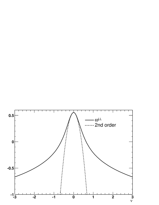
Figure 1: $\omega^{\mathrm{LL}}(\frac{1}{2}+i\nu)$ and the second order Taylor polynomial around $\nu=0$.

In Fig. 1 we have plotted $\omega^{\mathrm{LL}}(\frac{1}{2}+i\nu)$ for $\alpha_{s}=0.2$ and it is seen that there is a maximum at $\nu=0$. Therefore, the behaviour of the gluon Green’s function in the limit of $\Delta\to\infty$ is determined by the value of $\omega^{\mathrm{LL}}(\frac{1}{2})=4\ln 2\alpha_{s}N/\pi$. A saddle point approximation based on the second order Taylor polynomial around $\nu=0$ will correctly describe the asymptotic exponential growth in $\Delta$, since the polynomial attains the correct value at the maximum.

1.2 Next-to-Leading Logarithmic Accuracy

When trying to extend this analysis to NLL accuracy one is immediately faced with the complications introduced by the breaking of the conformal invariance by the running coupling terms. This effect will necessarily change the eigenfunctions, and thus far the eigenfunctions for the full NLL kernel in QCD have not been constructed. Traditionally, the kernel at NLL has been studied using the projection on the Born level eigenfunctions as in Eq. (9). One finds $\!{}^{{\bf?}}$

$$\begin{split}\omega^{\mathrm{NLL}}(\gamma)\equiv&\int\mathrm{d}^{D-2}\mathbf{k}\ \mathcal{K}^{\mathrm{NLL}}\!\left({\bf k}_{a},{\bf k}\right)\left(\frac{\mathbf{k}^{2}}{\mathbf{k}_{a}^{2}}\right)^{\gamma-1}\\ =&\frac{\alpha_{s}(\mathbf{k}_{a}^{2})N}{\pi}\left(\chi^{\mathrm{LL}}(\gamma)+\chi^{\mathrm{NLL}}(\gamma)\frac{\alpha_{s}(\mathbf{k}_{a}^{2})N}{\pi}\right)\end{split}$$ (10)

with

$$\begin{split}\chi^{\mathrm{NLL}}(\gamma)=&-\frac{1}{4}\Big{[}\left(\frac{11}{3}-\frac{2}{3}\frac{n_{f}}{N}\right)\frac{1}{2}\left(\chi^{\mathrm{LL}}(\gamma)-\psi^{\prime}(\gamma)+\psi^{\prime}(1-\gamma)\right)\\ &-6\zeta(3)+\frac{\pi^{2}\cos(\pi\gamma)}{\sin^{2}(\pi\gamma)(1-2\gamma)}\left(3+\left(1+\frac{n_{f}}{N^{3}}\right)\frac{2+3\gamma(1-\gamma)}{(3-2\gamma)(1+2\gamma)}\right)\\ &-\left(\frac{67}{9}-\frac{\pi^{2}}{3}-\frac{10}{9}\frac{n_{f}}{N}\right)\chi^{\mathrm{LL}}-\psi^{\prime\prime}(\gamma)-\psi^{\prime\prime}(1-\gamma)-\frac{\pi^{3}}{\sin(\pi\gamma)}+4\phi(\gamma)\Big{]},\end{split}$$ (11)

where

$$\begin{split}\phi(\gamma)=&-\int_{0}^{1}\frac{\mathrm{d}x}{1+x}(x^{\gamma-1}+x^{-\gamma})\int_{x}^{1}\frac{\mathrm{d}t}{t}\ln(1-t)\\ =&\sum_{n=0}^{\infty}(-1)^{n}\left[\frac{\psi(n+1+\gamma)-\psi(1)}{(n+\gamma)^{2}}+\frac{\psi(n+2-\gamma)-\psi(1)}{(n+1-\gamma)^{2}}\right].\end{split}$$ (12)

An approximation to the gluon Green’s function at NLL can then be constructed by use of $\omega^{\mathrm{NLL}}$ in place of $\omega^{\mathrm{LL}}$ in Eq. (8). We have in Fig. 2 plotted the real and imaginary part of $\omega^{\mathrm{NLL}}$ compared with $\omega^{\mathrm{LL}}$ for $\alpha_{s}=0.2$. The double hump structure of the real part of $\omega^{\mathrm{NLL}}$ is potentially a disaster for the gluon Green’s function. At asymptotically large $\Delta$ the behaviour of the gluon Green’s function is determined by the position and value of the maxima of $\omega^{\mathrm{NLL}}$ only. Since there are two such distinct maxima located at $\gamma_{1}=1/2-i\nu_{0},\gamma_{2}=1/2+i\nu_{0}$, the asymptotic estimate of the NLL gluon Green’s function based on the LL eigenfunctions will have an oscillatory behaviour in $\ln k_{a}/k_{b}$. This is a problem of matching to the DGLAP evolution, and is a problem strictly outside the Regge kinematics.

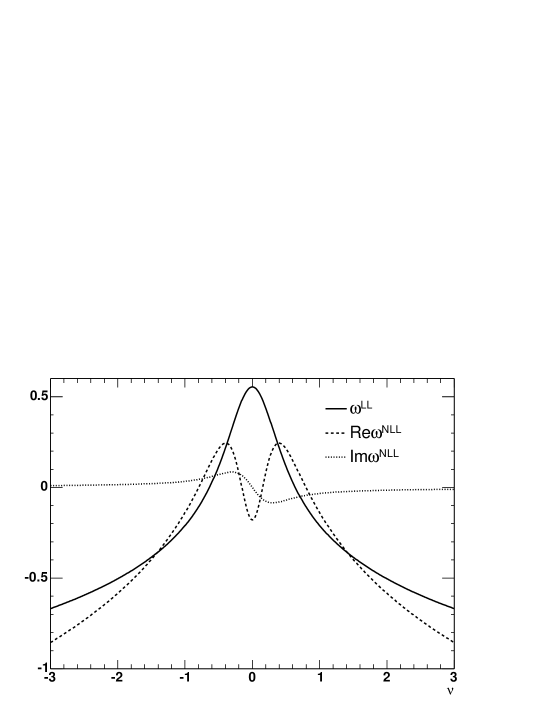
Figure 2: $\omega^{\mathrm{LL}}(\frac{1}{2}+i\nu)$ and $\omega^{\mathrm{NLL}}(\frac{1}{2}+i\nu)$ for $\alpha_{s}=0.2$, and $N=n_{f}=3$.

The initial observation of the large NLL corrections was based on the difference $\omega^{\mathrm{LL}}-\omega^{\mathrm{NLL}}$ evaluated at $\nu=0$. Indeed, for reasonable values of the coupling, the real part of $\omega^{\mathrm{NLL}}$ is even negative at this point. However, this is not what determines the intercept. If indeed the solution of the BFKL equation at NLL was obtained using $\omega^{\mathrm{NLL}}$ of Eq. (10), then the asymptotic intercept at NLL would again be determined by the maximum value attained by the real part of $\omega^{\mathrm{NLL}}(\gamma)$ along the contour $\gamma=1/2+i\nu$. We see from Fig. 2 that this maximum value is roughly halved compared to the LL asymptotic intercept.

However, even within the Regge kinematics, this analysis leads to severe problems in the very limit, where the resummed logarithmic terms are meant to dominate the scattering matrix. The non-zero imaginary part of $\omega^{\mathrm{NLL}}(\frac{1}{2}+i\nu_{0})$ leads to oscillations with increasing rapidity for any choice of $k_{a}$ and $k_{b}$! This clearly signals a breakdown of the approach in the very limit it is meant to describe.

The solution to this apparent problem is the realisation that what one has studied with this method is indeed not the true solution to the BFKL equation at NLL. The LL eigenfunctions are not the eigenfunctions at NLL (for non-zero $\beta_{0}$). Indeed, the only contribution to the troublesome imaginary part of $\omega^{\mathrm{NLL}}(\gamma)$ for $\gamma=1/2+i\nu$ stems from the term $-\psi^{\prime}(\gamma)+\psi(1-\gamma)$ in Eq. (11), which contributes to $\omega^{\mathrm{NLL}}$ with a factor proportional to $\beta_{0}$ (that is, it vanishes in the limit where the LL eigenfunctions diagonalises the NLL kernel). It was observed already in Ref.$\!{}^{{\bf?}}$ that this part of the NLL corrections is the only one that is not symmetric under $\gamma\leftrightarrow 1-\gamma$, and that if one expands the kernel on the LL eigenfunctions rescaled by a square root of the coupling, i.e. $(k^{2})^{\gamma-1}\left(\frac{\alpha_{s}(k^{s})}{\alpha_{s}(\mu^{2})}\right)^{-1/2}$ then these and only these terms would disappear from Eq. (11). What was perhaps not realised is that since this is the only contribution to the imaginary part of $\omega^{\mathrm{NLL}}$, this would simultaneously cure the problem of oscillations within the Regge-limit. It should be emphasised though that these rescaled functions still are not the true eigenfunctions at NLL, but it is straightforward to check numerically that the “off-diagonal elements” of $\omega^{\mathrm{NLL}}$ (i.e. those obtained with a different $\gamma$ for $k_{a}$ and $k$ in Eq. (10)) are far smaller in this case than when using the pure LL eigenfunctions. With the advance of new approaches to the solution of the BFKL equation at full NLL accuracy$\!{}^{{\bf?},{\bf?},{\bf?},{\bf?}}$ it has also been possible to check explicitly how well the two approximations compare with the full solution. We find that the approximation using the rescaled LL eigenfunctions is much closer to the true solution than the one using the pure LL ones. It should be noted that a saddle point approximation based around $\nu=0$ would have to use an extremely large order approximation in order to describe correctly the asymptotic intercept. Even the 16th order Taylor polynomial would fail to reach the maximum value for $\omega^{\mathrm{NLL}}$ in Fig. 2. It would be far better to base a saddle point approximation around $\nu_{0}$.

Using the guess obtained from these rescaled eigenfunctions it is possible to calculate the intercept as the logarithmic derivative of the gluon Green’s function for fixed $k_{a}$ and $k_{b}$, as a function of the rapidity. This is depicted on Fig. 3. We see that although the NLL correction amounts to roughly a factor of two, it is stable. Also, it should be remembered that the study of both the LL and NLL intercept here has been performed without constraining the phase space of the BFKL resummation to such which is attainable at a given collider. The effects of such a constrain are known to be large$\!{}^{{\bf?},{\bf?},{\bf?},{\bf?},{\bf?},{\bf?}}$ and reduce the LL evolution significantly (and presumably the NLL intercept to a slightly lesser extent).

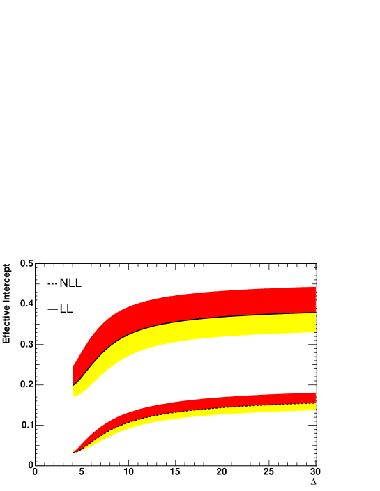
Figure 3: The effective intercept (of $f(k_{a}=20\mathrm{GeV},k_{b}=30\mathrm{GeV},\Delta)$ with $\alpha_{s}(30\mathrm{GeV})=0.15$), as a function of the rapidity at LL (upper line) and NLL (lower line). The uncertainty due to a renormalisation scale variation of a factor of two is indicated by the colour band.

Conclusions

We have shown that the NLL corrections to the BFKL intercept are large but stable within the Regge kinematics. The instability with respect to the evolution in rapidity observed in initial analyses is a direct result of using the conformal set of leading log eigenfunctions as if they were eigenfunctions at NLL. Indeed, for $\beta_{0}=0$ this instability disappear even in this analysis, and this the case also for non-zero $\beta_{0}$ if one applies rescaled eigenfunctions. Although these still do not diagonalise the kernel at NLL, the results obtained using the rescaled eigenfunctions describe the full solution obtained numerically much better than the approximation obtain using just the LL eigenfunctions. In the conformal limit of $\beta_{0}=0$, where the NLL corrections can be studied exactly using the projections on the LL eigenfunctions, any modification of the NLL kernel to match better to the DGLAP region (like the ones of Ref.$\!{}^{{\bf?},{\bf?}}$) must move the position of the maximum of $\omega^{\mathrm{NLL}}$ to $\nu=0$ while not changing the maximum value itself significantly (since this would lead to a change in the asymptotic intercept obtained within the Regge kinematic).

References

References

-
[1]
L. N. Lipatov,
Sov. J. Nucl. Phys. 23 (1976) 338
[Yad. Fiz. 23 (1976) 642],
E. A. Kuraev, L. N. Lipatov and V. S. Fadin, Sov. Phys. JETP 45 (1977) 199 [Zh. Eksp. Teor. Fiz. 72 (1977) 377],
I. I. Balitsky and L. N. Lipatov, Sov. J. Nucl. Phys. 28 (1978) 822 [Yad. Fiz. 28 (1978) 1597] - [2] V. S. Fadin and L. N. Lipatov, Phys. Lett. B 429 (1998) 127
- [3] J. R. Andersen and A. Sabio Vera, Phys. Lett. B 567 (2003) 116
- [4] J. R. Andersen and A. Sabio Vera, Nucl. Phys. B 679 (2004) 345
- [5] J. R. Andersen and A. Sabio Vera, Nucl. Phys. B 699 (2004) 90
- [6] M. Ciafaloni, D. Colferai, G. P. Salam and A. M. Stasto, Phys. Rev. D 68 (2003) 114003
- [7] J. R. Andersen and W. J. Stirling, JHEP 0302 (2003) 018
- [8] L. H. Orr and W. J. Stirling, Phys. Rev. D 56 (1997) 5875
- [9] L. H. Orr and W. J. Stirling, Phys. Lett. B 429 (1998) 135
- [10] L. H. Orr and W. J. Stirling, Phys. Lett. B 436, 372 (1998)
- [11] J. R. Andersen, V. Del Duca, F. Maltoni and W. J. Stirling, JHEP 0105 (2001) 048
- [12] J. R. Andersen, V. Del Duca, S. Frixione, C. R. Schmidt and W. J. Stirling, JHEP 0102 (2001) 007
- [13] G. P. Salam, JHEP 9807 (1998) 019 [arXiv:hep-ph/9806482].
- [14] A. S. Vera, “An all-poles approximation to collinear resummations in the Regge limit of perturbative QCD,” arXiv:hep-ph/0505128.