Top quark physics in hadron collisions

Abstract

The top quark is the heaviest elementary particle observed to date. Its large mass makes the top quark an ideal laboratory to test predictions of perturbation theory concerning heavy quark production at hadron colliders. The top quark is also a powerful probe for new phenomena beyond the Standard Model of particle physics. In addition, the top quark mass is a crucial parameter for scrutinizing the Standard Model in electroweak precision tests and for predicting the mass of the yet unobserved Higgs boson. Ten years after the discovery of the top quark at the Fermilab Tevatron top quark physics has entered an era where detailed measurements of top quark properties are undertaken. In this review article an introduction to the phenomenology of top quark production in hadron collisions is given, the lessons learned in Tevatron Run I are summarized, and first Run II results are discussed. A brief outlook to the possibilities of top quark research a the Large Hadron Collider, currently under construction at CERN, is included.

1 Introduction

The top quark is the by far heaviest of the six fundamental fermions in the Standard Model (SM) of particle physics. Its large mass made the search for the top quark a long and tedious process, since accelerators with high centre-of-mass energies are needed. In 1977 the discovery of the bottom quark indicated the existence of a third quark generation, and shortly thereafter the quest for the top quark began. Searches were conducted in electron-positron ($e^{+}e^{-}$) and proton-antiproton ($p\bar{p}$) collisions during the 1980s and early 1990s. Finally, in 1995 the top quark was discovered at the Fermilab Tevatron $p\bar{p}$ collider. Subsequently, its mass was precisely measured to be $M_{\mathrm{top}}=(178.0\pm 4.3)\,\mathrm{GeV}/c^{2}$ [1]. The relative precision of this measurement (2.4%) is better than our knowledge of any other quark mass. The top quark is about 40 times heavier than the second-heaviest quark, the bottom quark. Its huge mass makes the top quark an ideal probe for new physics beyond the SM. It remains an open question to particle physics research whether the observed mass hierarchy is a result of unknown fundamental particle dynamics. It has been argued that the top quark could be the key to understand the dynamical origin of how particle masses are generated by the mechanism of electroweak symmetry breaking, since its mass is close to the energy scale at which the break down occurs (vacuum expectation value of the Higgs field = 246 GeV) [2]. The most favoured framework to describe electroweak symmetry breaking is the Higgs mechanism. The masses of the Higgs boson, the $W$ boson and the top quark are closely related through higher order corrections to various physics processes. A precise knowledge of the top quark mass together with other electroweak precision measurements can therefore be used to predict the Higgs boson mass.

At present, top quarks can only be directly produced at the Tevatron. The physics results of the Tevatron experiments CDF and DØ will therefore be the focus of this article. We review the experimental status of top quark physics at the beginning of the Tevatron Run II which will yield considerably improved measurements in the top sector. We discuss the first Run II analysis results and summarise the lessons learned from Run I data taken between 1990 – 1995.

The outline of this article is as follows: In chapter 2 we give a brief introduction to the SM of particle physics and stress the importance of the top quark for higher order corrections to electroweak perturbation theory. In particular, we discuss electroweak precision measurements used to predict the top quark and Higgs boson mass within the SM. Chapter 3 covers the theoretical description of SM top quark production at hadron colliders and the top quark decay. In chapter 4 we elaborate on analysis techniques used to detect top quarks in particle detectors. A short description of the Tevatron experiments CDF and DØ  is provided. In chapter 5 we recall the early searches for the top quark in the 1980s and the discovery at the Tevatron in 1994/95. In chapter 6 we present various techniques to measure the top-antitop pair production cross section. Chapter 7 covers the top quark mass measurements and chapter 8 summarises various advanced tests of top quark properties. In chapter 9 we discuss the search for anomalous (non SM) top quark production. Previous reviews of top quark physics can be found in references [3, 4, 5, 6, 7, 8, 9].

2 The top quark in the Standard Model

2.1 The standard model of particle physics

The Standard Model (SM) of particle physics postulates that all matter be composed of a few basic, point-like and structureless constituents: elementary particles. One distinguishes two groups: quarks and leptons. Both of them are fermions and carry spin 1/2. The quarks come in six different flavours: up, down, charm, strange, top and bottom; formally described by assigning flavour quantum numbers. The SM incorporates six leptons: the electron ($e^{-}$) and the electron-neutrino ($\nu_{e}$), the muon ($\mu^{-}$) and the muon-neutrino ($\nu_{\mu}$), the tau ($\tau^{-}$) and the tau-neutrino ($\nu_{\tau}$). They carry electron, muon and tau quantum numbers. Quarks and leptons can be grouped into three generations (or families) as shown in table 1 which also contains the charges and masses of the particles.

Table 1: Three generations of quarks and leptons, their charges and masses are given [10].

$\begin{array}[]{cccrcrr}\hline\cr&\lx@intercol\hfil\mathrm{Quarks}\hfil\lx@intercol&\lx@intercol\hfil\mathrm{Leptons}\hfil\lx@intercol\\ \mathrm{Generation}&\mathrm{Symbol}&\mathrm{Charge}&\mathrm{Mass\;[MeV/}c^{2}]&\mathrm{Symbol}&\mathrm{Charge}&\mathrm{Mass\;[MeV/}c^{2}]\\ \hline\cr\mathbf{1}&u&+\frac{2}{3}&1.5\ \mathrm{to}\ 4&\nu_{e}&0&<3\cdot 10^{-6}\\ \mathbf{1}&d&-\frac{1}{3}&4\ \mathrm{to}\ 8&e^{-}&-1&0.51\\ \hline\cr\mathbf{2}&c&+\frac{2}{3}&(1.15\ \mathrm{to}\ 1.35)\cdot 10^{3}&\nu_{\mu}&0&<0.19\\ \mathbf{2}&s&-\frac{1}{3}&80\ \mathrm{to}\ 130&\mu^{-}&-1&106\\ \hline\cr\mathbf{3}&t&+\frac{2}{3}&(178.0\pm 4.3)\cdot 10^{3}&\nu_{\tau}&0&<18.2\\ \mathbf{3}&b&-\frac{1}{3}&(4.1\ \mathrm{to}\ 4.4)\cdot 10^{3}&\tau^{-}&-1&1777\\ \hline\cr\end{array}$

The three generations exhibit a striking mass hierarchy, the top quark having by far the highest mass. Understanding the deeper reason behind the hierarchy and generation structure is one of the open questions of particle physics. Each quark and each lepton has an associated antiparticle with the same mass but opposite charge. The antiquarks are denoted $\bar{u}$, $\bar{d}$, etc. The antiparticle of the electron is the positron ($e^{+}$).

The forces of nature acting between quarks and leptons are described by quantized fields. The interactions between elementary particles are due to the exchange of field quanta which are said to mediate the forces. The SM incorporates the electromagnetic force, responsible for example for the emission of light from excited atoms, the weak force, which for instance causes nuclear beta decay, and the strong force which keeps nuclei stable. Gravitation is not included in the framework of the SM but rather described by the theory of general relativity. All particles with mass or energy feel the gravitational force. However, due to the weakness of gravitation with respect to the other forces acting in elementary particle reactions it is not further considered in this article. The electromagnetic, weak and strong forces are described by so called quantum gauge field theories (see explanation below). The quanta of these fields carry spin 1 and are therefore called gauge bosons. The electromagnetic force is mediated by the massless photon ($\gamma$), the weak force by the massive $W^{\pm}$, $M_{W}=(80.425\pm 0.038)$ GeV/$c^{2}$ [10], and the $Z^{0}$, $M_{Z}=(91.1876\pm 0.0021)$ GeV/$c^{2}$ [10], and the strong force by eight massless gluons (g). Quarks participate in electromagnetic, weak and strong interactions. All leptons experience the weak force, the charged ones also feel the electromagnetic force. But leptons do not take part in strong interactions. A thorough introduction to the SM can be found in various text books of particle physics [11, 12, 13, 14, 15].

2.1.1 Electroweak interactions.

In quantum field theory quarks and leptons are represented by spinor fields $\boldsymbol{\Psi}$ which are functions of the continuous space-time coordinates $x_{\mu}$. To take into account that the weak interaction only couples to the left-handed particles, left- and right-handed fields $\boldsymbol{\Psi}_{\mathbf{L}}=\frac{1}{2}(1-\gamma_{5})\,\boldsymbol{\Psi}$ and $\boldsymbol{\Psi}_{\mathbf{R}}=\frac{1}{2}(1+\gamma_{5})\,\boldsymbol{\Psi}$ are introduced. The left-handed states of one generation are grouped into weak-isospin doublets, the right-handed states form singlets:

$$\begin{array}[]{cccccccc}\left(\begin{array}[]{c}u\\ d\\ \end{array}\right)_{L}&\left(\begin{array}[]{c}c\\ s\\ \end{array}\right)_{L}&\left(\begin{array}[]{c}t\\ b\\ \end{array}\right)_{L}&&&\left(\begin{array}[]{c}\nu_{e}\\ e\\ \end{array}\right)_{L}&\left(\begin{array}[]{c}\nu_{\mu}\\ \mu\\ \end{array}\right)_{L}&\left(\begin{array}[]{c}\nu_{\tau}\\ \tau\\ \end{array}\right)_{L}\\ &&\\ u_{R}&c_{R}&t_{R}&&&&&\\ d_{R}&s_{R}&b_{R}&&&e_{R}&\mu_{R}&\tau_{R}\\ \end{array}$$

The weak-isospin assignment for the doublet is: up-type quarks (u,c,t) and neutrinos carry $T_{3}=+\frac{1}{2}$; down-type quarks (d,s,b), electron, muon and tau lepton have $T_{3}=-\frac{1}{2}$. In the original SM the right-handed neutrino states are omitted, since neutrinos are assumed to be massless. Recent experimental evidence [16, 17, 18], however, strongly indicates that neutrinos have mass and the SM needs to be extended in this respect.

The dynamics of the electromagnetic and weak forces follow from the free particle Lagrangian density

$$\mathcal{L}_{0}=\rmi\;\overline{\boldsymbol{\Psi}}\;\gamma^{\mu}\partial_{\mu}\;\boldsymbol{\Psi}$$ (1)

by demanding the invariance of $\mathcal{L}_{0}$ under local phase transformations:

$$\boldsymbol{\Psi}_{\mathbf{L}}\longrightarrow\rme^{\rmi g\boldsymbol{\alpha}(x)\mathbf{\cdot T}+\rmi g^{\prime}\beta(x)Y}\;\boldsymbol{\Psi}_{\mathbf{L}}\ \ \ \ \ \mathrm{and}\ \ \ \ \ \boldsymbol{\Psi}_{\mathbf{R}}\longrightarrow\rme^{\rmi g^{\prime}\beta(x)Y}\;\boldsymbol{\Psi}_{\mathbf{R}}\;.$$ (2)

For historical reasons these transformations are also referred to as gauge transformations. In (2) the parameter $\boldsymbol{\alpha}(x)$ is an arbitrary three-component vector and $\mathbf{T}=(T_{1},\,T_{2},\,T_{3})^{t}$ is the weak-isospin operator whose components $T_{i}$ are the generators of $SU(2)_{L}$ symmetry transformations. The index $L$ indicates that the phase transformations act only on left-handed states. The matrix representations are given by $T_{i}=\frac{1}{2}\;\tau_{i}$ where the $\tau_{i}$ are the Pauli matrices. The $T_{i}$ do not commute: $[T_{i},T_{j}]=\rmi\,\epsilon_{ijk}\,T_{k}$. That is why the $SU(2)_{L}$ gauge group is said to be non-Abelian. $\beta(x)$ is a one-dimensional function of $x$. $Y$ is the weak hypercharge which satisfies the relation $Q=T_{3}+Y/2$, where $Q$ is the electromagnetic charge. $Y$ is the generator of the symmetry group $U(1)_{Y}$. Demanding the Lagrangian $\mathcal{L}_{0}$ to be invariant under the combined gauge transformations of $SU(2)_{L}\times U(1)_{Y}$, see (2), requires the addition of terms to the free Lagrangian which involve four additional vector (spin 1) fields: the isotriplet $\mathbf{W_{\mu}}=(W_{1\,\mu}\,,W_{2\,\mu}\,,W_{3\,\mu})^{t}$ for $SU(2)_{L}$ and the singlet $B_{\mu}$ for $U(1)_{Y}$. This is technically done by replacing the derivative $\partial_{\mu}$ in $\mathcal{L}_{0}$ by the covariant derivative

$$D_{\mu}=\partial_{\mu}+\rmi\,g\,\mathbf{W_{\mu}\cdot T}+\rmi\,g^{\prime}\frac{1}{2}B_{\mu}Y$$ (3)

and adding the kinetic energy terms of the gauge fields: $-\frac{1}{4}\mathbf{W_{\mu\nu}\cdot W^{\mu\nu}}-\frac{1}{4}B_{\mu\nu}\mathbf{\cdot}B^{\mu\nu}$. The field tensors $\mathbf{W_{\mu\nu}}$ and $B_{\mu\nu}$ are given by $\mathbf{W_{\mu\nu}}=\partial_{\mu}\mathbf{W_{\nu}}-\partial_{\nu}\mathbf{W_{\mu}}-g\cdot\mathbf{W_{\mu}\times W_{\nu}}$ and $B_{\mu\nu}=\partial_{\mu}B_{\nu}-\partial_{\nu}B_{\mu}$. Since the vector fields $\mathbf{W_{\mu}}$ and $B_{\mu}$ are introduced via gauge transformations they are called gauge fields and the quanta of these fields are named gauge bosons. For an electron-neutrino pair, for example, the resulting Lagrangian is:

$$\mathcal{L}_{1} = \rmi\;\overline{\left(\begin{array}[]{c}\nu_{e}\\ e\end{array}\right)}_{L}\;\gamma^{\mu}\left[\partial_{\mu}+\rmi\,g\,\mathbf{W_{\mu}\cdot T}+\rmi\,g^{\prime}\,Y_{L}\,\frac{1}{2}\,B_{\mu}\right]\left(\begin{array}[]{c}\nu_{e}\\ e\end{array}\right)_{L}+$$ (9)

$$\rmi\;\bar{e}_{R}\;\gamma^{\mu}\left[\partial_{\mu}-g^{\prime}\,Y_{R}\,\frac{1}{2}\,B_{\mu}\right]e_{R}-\frac{1}{4}\;\mathbf{W_{\mu\nu}\cdot W^{\mu\nu}}-\frac{1}{4}B_{\mu\nu}\mathbf{\cdot}B^{\mu\nu}$$

This model developed by Glashow [19], Weinberg and Salam [20, 21] in the 1960s allows to describe electromagnetic and weak interactions in one framework. One therefore refers to it as unified electroweak theory.

2.1.2 The Higgs mechanism.

One has to note, however, that $\mathcal{L}_{1}$ describes only massless gauge bosons and massless fermions. Mass-terms such as $\frac{1}{2}M^{2}B_{\mu}B^{\mu}$ or $-m\overline{\boldsymbol{\Psi}}\boldsymbol{\Psi}$ are not gauge invariant and therefore cannot be added. To include massive particles into the model in a gauge invariant way the Higgs mechanism is used. Four scalar fields are added to the theory in form of the isospin doublet $\mathbf{\Phi}=\left(\phi^{+},\;\phi^{0}\right)^{t}$ where $\phi^{+}$ and $\phi^{0}$ are complex fields. This is the minimal choice. The term $\mathcal{L}_{H}=\left|D_{\mu}\boldsymbol{\Phi}\right|^{2}-V({\boldsymbol{\Phi}}^{\dagger}\boldsymbol{\Phi})$ is added to $\mathcal{L}_{1}$. The scalar potential takes the form $V({\boldsymbol{\Phi}}^{\dagger}\boldsymbol{\Phi})=\mu^{2}\;{\mathbf{\Phi}}^{\dagger}\mathbf{\Phi}+\lambda\;({\boldsymbol{\Phi}}^{\dagger}\boldsymbol{\Phi})^{2}$.

In most cases particle reactions cannot be calculated from first principles. One rather has to use perturbation theory and expand a solution starting from the ground state of the system which is in particle physics called the vacuum expectation value. The parameters $\mu$ and $\lambda$ can be chosen such that the vacuum expectation value of the Higgs potential $V$ is different from zero: $|\boldsymbol{\Phi}_{\mathrm{vac}}|=\sqrt{-\frac{1}{2}\,\mu^{2}/\lambda}$ and thus does not share the symmetry of $V$. The scalar Higgs fields inside $\boldsymbol{\Phi}$ are redefined such that the new fields, $\boldsymbol{\xi}(x)=(\xi_{1}(x),\xi_{2}(x),\xi_{3}(x))^{t}$ and $H(x)$, have zero vacuum expectation value. When the new parameterization of $\mathbf{\Phi}$ is inserted into the Lagrangian, the symmetry of the Lagrangian is broken, that is, the Lagrangian is not an even function of the Higgs fields anymore. This mechanism where the ground states do not share the symmetry of the Lagrangian is called spontaneous symmetry breaking. As a result, one of the Higgs fields, the $H(x)$ field, has acquired mass, while the other three fields, $\boldsymbol{\xi}$, remain massless [22, 23].

Applying spontaneous symmetry breaking as described above to the combined Lagrangian $\mathcal{L}_{2}=\mathcal{L}_{1}+\mathcal{L}_{H}$ and enforcing local gauge invariance of $\mathcal{L}_{2}$, makes three electroweak gauge bosons acquire mass. This is the aim of the whole formalism. One field, the photon field, remains massless. The resulting boson fields after spontaneous symmetry breaking are, however, not the original fields $\mathbf{W_{\mu}}$ and $B_{\mu}$ but rather mixtures of those: the $W^{\pm}_{\mu}=(W^{1}_{\mu}\mp\rmi\;W^{2}_{\mu})/\sqrt{2}$, the $Z^{0}$ and the photon field $A_{\mu}$:

$$\left(\begin{array}[]{c}A_{\mu}\\ Z_{\mu}\end{array}\right)=\left(\begin{array}[]{cc}\cos\theta_{W}&\sin\theta_{W}\\ -\sin\theta_{W}&\cos\theta_{W}\end{array}\right)\ \ \left(\begin{array}[]{c}B_{\mu}\\ W^{3}_{\mu}\end{array}\right)$$ (10)

The mixing angle $\theta_{W}$ is the Weinberg angle defined by the coupling constants $g^{\prime}/g=\tan\theta_{W}$. While the original massless vector fields have two degrees of freedom (transverse polarizations), the new massive fields acquired a third degree of freedom, their longitudinal polarization. The longitudinal modes of the $W^{\pm}$ and the $Z^{0}$ are due to the disappearance of the $\boldsymbol{\xi}$ states from the theory. The total number of degrees of freedom is thus conserved.

Spontaneous symmetry breaking also generates lepton masses if Yukawa interaction terms of the lepton and Higgs fields are added to the Lagrangian:

$$\mathcal{L}_{\mathrm{Yukawa}}^{\mathrm{lepton}}=-G_{e}\left[\bar{e}_{R}\left(\mathbf{\Phi}^{\dagger}\left(\begin{array}[]{c}\nu_{e}\\ e\end{array}\right)_{L}\right)+\left(\overline{\left(\nu_{e},e\right)}^{t}_{L}\mathbf{\Phi}\right)\ e_{R}\right]$$ (11)

Here the Yukawa terms for the electron-neutrino doublet are given as an example. $G_{e}$ is a further coupling constant describing the coupling of the electron and electron-neutrino to the Higgs field. In this formalism neutrinos are assumed to be massless.

Quark masses are also generated by adding Yukawa terms to the Lagrangian. However, for the quarks both, the upper and the lower member of the weak-isospin doublet, need to acquire mass. For this to happen an additional conjugate Higgs multiplet has to be constructed: $\boldsymbol{\Phi}_{c}=\rmi\tau_{2}\boldsymbol{\Phi}^{*}=(\phi^{0^{*}},-\phi^{-})^{t}$. The Yukawa terms for the quarks are given by:

$$\mathcal{L}_{\mathrm{Yukawa}}^{\mathrm{quark}}=\sum_{i=1}^{3}\sum_{j=1}^{3}\ \tilde{G}_{ij}\ \bar{u}_{iR}\tilde{\boldsymbol{\Phi}}^{\dagger}\ \left(\begin{array}[]{c}u_{j}\\ d_{j}\end{array}\right)_{L}+G_{ij}\ \bar{d}_{iR}\ \boldsymbol{\Phi}^{\dagger}\ \left(\begin{array}[]{c}u_{j}\\ d_{j}\end{array}\right)_{L}+\ \mathrm{h.c.}$$ (12)

The $u_{j}$ and $d_{j}$ are the weak eigenstates of the up-type ($u,\,c,\,t$) and the down-type ($d,\,s,\,b$) quarks, respectively. Couplings between quarks of different generations are allowed by this ansatz. After spontaneous symmetry breaking the Yukawa terms produce mass terms for the quarks which can be described by mass matrices in generation space: $\overline{(u_{1},u_{2},u_{3})}_{R}\;\mathcal{M}^{u}\;(u_{1},u_{2},u_{3})^{t}_{L}$ and $\overline{(d_{1},d_{2},d_{3})}_{R}\;\mathcal{M}^{d}\;(d_{1},d_{2},d_{3})^{t}_{L}$ with $\mathcal{M}_{ij}^{u}=|\boldsymbol{\Phi}_{\mathrm{vac}}|\cdot\tilde{G}_{ij}$ and $\mathcal{M}_{ij}^{d}=|\boldsymbol{\Phi}_{\mathrm{vac}}|\cdot G_{ij}$. The mass matrices are non-diagonal but can be diagonalized by unitary transformations, which essentially means to change basis from weak eigenstates to mass eigenstates, which are identical to the flavour eigenstates $u$, $c$, $t$ and $d$, $s$, $b$. In charged-current interactions ($W^{\pm}$ exchange) this leads to transitions between mass eigenstates of different generations referred to as generation mixing. It is possible to set weak and mass eigenstates equal for the up-type quarks and ascribe the mixing entirely to the down-type quarks:

$$\left(\begin{array}[]{ccc}d^{\prime}\\ s^{\prime}\\ b^{\prime}\end{array}\right)_{L}=\mathbf{V}\ \left(\begin{array}[]{ccc}d\\ s\\ b\end{array}\right)_{L}=\left(\begin{array}[]{ccc}V_{ud}&V_{us}&V_{ub}\\ V_{cd}&V_{cs}&V_{cb}\\ V_{td}&V_{ts}&V_{tb}\\ \end{array}\right)\left(\begin{array}[]{ccc}d\\ s\\ b\end{array}\right)_{L}$$ (13)

where $d^{\prime}$, $s^{\prime}$ and $b^{\prime}$ are the weak eigenstates. The mixing matrix $\mathbf{V}$ is called the Cabbibo-Kobayashi-Maskawa (CKM) matrix [24].

2.1.3 Strong interactions.

The theory of strong interactions is called quantum chromodynamics (QCD) since it attributes a colour charge to the quarks. There are three different types of strong charges (colours): “red”, “green” and “blue”. Strong interactions conserve the flavour of quarks. Leptons do not carry colour at all, they are inert with respect to strong interactions. QCD is a quantum field theory based on the non-Abelian gauge group $SU(3)_{C}$ of phase transformations on the quark colour fields. Invoking local gauge invariance of the Lagrangian yields eight massless gauge bosons: the gluons. The gauge symmetry is exact and not broken as in the case of weak interactions. Each gluon carries one unit of colour and one unit of anticolour. The strong force binds quarks together to form bound-states called hadrons. There are two groups of hadrons: mesons consisting of a quark and an antiquark and baryons built of either three quarks or three antiquarks. All hadrons are colour-singlet states. Quarks cannot exist as free particles. This experimental fact is summarised in the notion of quark confinement: quarks are confined to exist in hadrons.

2.2 Model predictions of top quark properties

In 1975 the tau lepton was the first particle of the third generation to be discovered [25]. Only two years later, in 1977, a new heavy meson, the $\Upsilon$, was discovered [26]. It was quickly recognised to contain a new fifth quark, the $b$ quark ($\Upsilon=b\bar{b}$). After these discoveries the doublet structure of the SM strongly suggested the existence of a third neutrino associated with the tau lepton and the existence of a sixth quark, called the top quark. The properties of the $b$ quark and $b$ hadrons were subject to extensive experimental research in the past 25 years. As a result, charge and weak isospin of the $b$ quark are well established quantities: $Q_{b}=-\frac{1}{3}$ and $T_{3}=-\frac{1}{2}$. The charge $Q_{b}$ was first deduced from measurements of the cross section $\sigma_{\mathrm{had}}$ for hadron production on the $\Upsilon$ resonance at the DORIS $e^{+}e^{-}$ storage ring [27, 28, 29]. The integral over $\sigma_{\mathrm{had}}$ is related to the leptonic width $\Gamma_{ee}$ of the $\Upsilon$: $\int\sigma_{\mathrm{had}}\,\rmd M=6\,\pi^{2}\Gamma_{ee}/M_{\Upsilon}^{2}$ (using the approximation that $\Gamma_{\mathrm{had}}\approx\Gamma_{\mathrm{total}}$). Nonrelativistic potential models of the $\Upsilon$ relate $\Gamma_{ee}$ to the charge of the constituent $b$ quarks.

The weak isospin of the $b$ quark was obtained from the measurement of the forward-backward asymmetry $A_{\mathrm{FB}}$ in $e^{+}e^{-}\rightarrow b\bar{b}$ reactions. The asymmetry is defined as the difference in rate of $b$ quarks produced in the forward hemisphere (polar angle $\theta>90^{\circ}$) minus the rate of $b$ quarks produced in the backward hemisphere ($\theta<90^{\circ}$) over the sum of the two rates. In 1984 the JADE experiment measured $A_{\mathrm{FB}}=(-22.8\pm 6.0\pm 2.5)\%$ [30] in excellent agreement with the value of -25.2% predicted for a $b$ quark that is the lower member of a SM weak isospin doublet. In case of a weak isospin singlet the asymmetry would be zero. The assignment of quantum numbers for the $b$ quark allows to predict the charge and the weak isospin of the top quark to be: $Q_{t}=+\frac{2}{3}$ and $T_{3}=+\frac{1}{2}$.

Another argument which supported the existence of a complete third quark generation comes from perturbation theory. In particle physics the terms of a perturbation series are depicted in Feynman diagrams. The first order terms are pictured as tree level diagrams. Higher order terms correspond to loop diagrams. Certain loop diagrams are divergent. These divergencies can only be overcome by summing up over several divergent terms in a consistent manner and have the divergencies cancel each other. This formalism is called renormalization. For electroweak theory to be renormalizable, the sum over fermion triangle diagrams, such as the one shown in figure 1a, has to vanish [31, 32, 33]. With a third lepton doublet in place the cancellation only occurs if also a complete third quark doublet is there. While the SM predicts the charge and the weak isospin of the top quark, its mass remains a free parameter.

2.3 Top quark mass and electroweak precision measurements

Even though the top quark mass is not predicted by the SM it enters as a parameter in the calculation of radiative corrections to electroweak processes. With highly precise measurements at hand it is therefore possible to indirectly determine the top quark mass from those processes [34, 35]. In this context radiative corrections denote higher order contributions to a perturbation series, e.g. to calculate cross sections of electroweak processes.

The most precise electroweak measurements are available from $e^{+}e^{-}$ colliders operating at the $Z^{0}$ pole, where $\sqrt{s}=M_{Z}$. Here $\sqrt{s}$ is the centre-of-mass energy of the colliding electrons and positrons. $M_{Z}$ is the mass of the $Z^{0}$ boson. In the 1990s there were two particle colliders operating on the $Z^{0}$ pole: the Large Electron Positron Collider (LEP) [36] at CERN with four experiments (ALEPH [37, 38], DELPHI [39, 40], L3 [41, 42] and OPAL [43]) and the Stanford Linear Collider (SLC) [44] with the SLD [45, 46] experiment. The LEP experiments collected about 4 million $Z^{0}$ events each, SLD on the order of 0.5 million events. Although the SLD sample is considerably smaller, the experiment reached a competitive sensitivity for many measurements, since at SLC it was possible to polarize the colliding electrons and positrons.

Two examples of radiative corrections to the $Z^{0}$ propagator and to the $Z^{0}$ vertex involving the top quark are given in figure 1b and 1c. The top mass plays a particular large role in the corrections represented by these diagrams due to the large mass difference between the top quark and its weak-isospin partner, the $b$ quark. The correction terms introduce a quadratic dependence on the top mass, whereas the dependence on the Higgs mass is only logarithmic.

(a)                                         (b)                                         (c)
              

Figure 1: (a) An example of a fermion triangle diagram. (b,c) Two example Feynman diagrams of radiative corrections involving the top quark. (b) is a radiative correction to the $Z^{0}$ propagator. (c) shows a vertex correction to the decay $Z^{0}\rightarrow b\bar{b}$.

The LEP electroweak working group (LEPEWWG) has combined the measurements of the four LEP experiments to obtain a common data set. To test SM predictions and check the overall consistency of the data with the model the SLD data and Tevatron measurements in $p\bar{p}$ collisions are included [47]. Among the results of the fits is an indirect determination of the top mass and indirect limits on the Higgs mass. The quantities used for a constraint fit to the SM are discussed below:

1. The mass $M_{Z}$ and the total width $\Gamma_{Z}$ of the $Z^{0}$. The definition of $M_{Z}$ and $\Gamma_{Z}$ is based on the Breit-Wigner denominator of the electroweak cross section for fermion pair ($f\bar{f}$) production due to $Z^{0}$ exchange: $\sigma_{f\bar{f}}(s)=\sigma^{0}_{f}\cdot s\Gamma_{Z}^{2}/((s-M_{Z}^{2})^{2}+(s\Gamma_{Z}/M_{Z})^{2})$ where $\sigma_{f}^{0}$ is the pole cross section at $\sqrt{s}=M_{Z}$.

2. The hadronic pole cross section:

   $$\sigma_{h}^{0}=\frac{12\;\pi}{M_{Z}^{2}}\cdot\frac{\Gamma_{ee}\,\Gamma_{\mathrm{had}}}{\Gamma_{Z}^{2}}$$

   where $\Gamma_{ee}$ and $\Gamma_{\mathrm{had}}$ are the partial widths for the $Z^{0}$ decaying into electrons or hadrons, respectively.

3. The ratio of the hadronic and leptonic widths at the $Z^{0}$ pole: $R_{\ell}^{0}\equiv\Gamma_{\mathrm{had}}/\Gamma_{\ell\ell}$. $\Gamma_{\ell\ell}$ is obtained from $Z^{0}$ decays into $e^{+}\,e^{-}$, $\mu^{+}\,\mu^{-}$ or $\tau^{+}\,\tau^{-}$ assuming lepton universality ($\Gamma_{ee}=\Gamma_{\mu\mu}=\Gamma_{\tau\tau}\equiv\Gamma_{\ell\ell}$) which is only correct for massless leptons. To account for the tau mass $\Gamma_{\tau\tau}$ is corrected, in average by $0.2\%$.

4. The pole forward-backward asymmetry $A_{\mathrm{FB}}^{0,\ell}$ ($\ell\in\{e,\mu,\tau\}$) for $Z^{0}$ decays into charged leptons. The asymmetry is defined as the total cross section for a negative lepton to be scattered into the forward direction ($90^{\circ}<\theta\leq 180^{\circ}$) minus the total cross section for a negative lepton to be scattered into the backward direction ($0^{\circ}\leq\theta\leq 90^{\circ}$) divided by the sum.

   $$A_{\mathrm{FB}}^{0,l}=\frac{\sigma_{\mathrm{F}}(\ell^{-},90^{\circ}<\theta\leq 180^{\circ})-\sigma_{\mathrm{B}}(\ell^{-},0^{\circ}\leq\theta\leq 90^{\circ})}{\sigma_{\mathrm{F}}(\ell^{-},90^{\circ}<\theta\leq 180^{\circ})+\sigma_{\mathrm{B}}(\ell^{-},0^{\circ}\leq\theta\leq 90^{\circ})}$$

   Here $\theta$ is the angle between the produced lepton and the incoming electron. The forward-backward asymmetry originates from parity violating terms in the total cross section. $A_{\mathrm{FB}}^{0,\ell}$ can be written as a combination of effective couplings $A_{\mathrm{FB}}^{0,\ell}=\frac{3}{4}\cdot\mathcal{A}_{e}\,\mathcal{A}_{\ell}$ with $\mathcal{A}_{\ell}=(2\;g_{V,\ell}\,g_{A,\ell})/(g_{V,\ell}^{2}+g_{A,\ell}^{2})$ where $g_{V,\ell}$ and $g_{A,\ell}$ are the vector and axial couplings, respectively.

5. The effective leptonic coupling $A_{\ell}$ derived from the tau polarization measurement. Parity violation in the weak interaction leads to longitudinally polarized final state fermions from the $Z^{0}$ decay. In case of the decay $Z^{0}\rightarrow\tau^{+}\tau^{-}$ this polarization can be measured via the subsequent parity violating decays of the tau as polarimeter. The polarization $P_{\tau}$ is defined in terms of the cross section for the production of right-handed and left-handed $\tau^{-}$, respectively: $P_{\tau}=(\sigma_{R}-\sigma_{L})/(\sigma_{R}+\sigma_{L})$. Averaging $P_{\tau}$ over all production angles $\theta$ gives a measure of the effective coupling: $\langle P_{\tau}\rangle=-\mathcal{A}_{\tau}$.

6. The effective leptonic weak mixing angle $\sin^{2}\theta^{\mathrm{lept}}_{\mathrm{eff}}$ from the inclusive hadronic charge asymmetry $\langle Q_{\mathrm{FB}}\rangle$ which is measured from $Z^{0}\rightarrow q\bar{q}$ decays. An estimator for the quark charge is derived from the sum of momentum weighted track charges in the quark and antiquark hemispheres, respectively.

7. The effective leptonic coupling $\mathcal{A}_{\ell}$ derived from left-right asymmetries measured with longitudinally polarized electron and positron beams at SLD. The left-right asymmetry $A_{\mathrm{LR}}$ is formed as the number of $Z^{0}$ bosons $N_{L}$ produced by left-handed electrons minus the number of $Z^{0}$ bosons $N_{R}$ produced by right-handed electrons:

   $$A_{\mathrm{LR}}=\frac{N_{L}-N_{R}}{N_{L}+N_{R}}\cdot\frac{1}{P_{e}}$$

   Additionally, one divides by the luminosity weighted polarization $P_{e}$ of the electron beam. $A_{\mathrm{LR}}$ is measured for all three charged lepton final states. The pole values $A_{\mathrm{LR}}^{0}$ are equivalent to the effective couplings $\mathcal{A}_{e}$, $\mathcal{A}_{\mu}$ and $\mathcal{A}_{\tau}$, respectively. Assuming lepton universality the results are combined to form a single value $A_{\ell}$.

8. The measurement of the top mass by CDF and DØ  [1].

9. The ratios of $b$ and $c$ quark partial widths of the $Z^{0}$ with respect to its total hadronic partial width: $R_{b}^{0}\equiv\Gamma_{b\bar{b}}/\Gamma_{\mathrm{had}}$ and $R_{c}^{0}\equiv\Gamma_{c\bar{c}}/\Gamma_{\mathrm{had}}$.

10. The forward-backward asymmetries for the decays $Z^{0}\rightarrow b\bar{b}$ and $Z^{0}\rightarrow c\bar{c}$: $A_{\mathrm{FB}}^{0,b}$ and $A_{\mathrm{FB}}^{0,c}$, defined analogously to the leptonic asymmetries.

11. The effective couplings for $b$ and $c$ quarks: $\mathcal{A}_{b}$ and $\mathcal{A}_{c}$, defined analogously to $\mathcal{A}_{\ell}$.

12. The mass and width of the $W$ boson from the combination of measurements in $p\bar{p}$ collisions by UA2, CDF and DØ and measurements at LEP 2.

The quantities describing the decay $Z^{0}\rightarrow b\bar{b}$ ($R_{b}^{0}$, $A_{\mathrm{FB}}^{0,b}$ and $\mathcal{A}_{b}$) exhibit a particular strong dependence on $M_{\mathrm{top}}$ because they are sensitive to weak vertex corrections as the one shown in figure 1c. In many cases vertex corrections involving a $W$ boson are suppressed due to small CKM matrix elements. The vertices in figure 1, however, contain the matrix element $V_{tb}$ which is close to 1. Therefore, the graphs lead to significant corrections depending on the top quark mass.

The measured values of the above listed quantities are given in table. 2.

Physical quantity	Measurement with total error	SM fit	Physical quantity	Measurement with total error	SM fit
LEP measurements			LEP and SLD heavy flavour
$M_{Z}$ [GeV/$c^{2}$]	91.1875 $\pm$ 0.0021	91.1875	$R_{b}^{0}$	0.21630 $\pm$ 0.00065	0.21562
$\Gamma_{Z}$ [GeV/$c^{2}$]	2.4952 $\pm$ 0.0023	2.4966	$R_{c}^{0}$	0.1723 $\pm$ 0.0031	0.1723
$\sigma_{h}^{0}$ [nb]	41.540 $\pm$ 0.037	41.481	$A_{\mathrm{FB}}^{\mathrm{0,\,b}}$	0.0998 $\pm$ 0.0017	0.1040
$R_{\ell}^{0}$	20.767 $\pm$ 0.025	20.739	$A_{\mathrm{FB}}^{\mathrm{0,\,c}}$	0.0706 $\pm$ 0.0035	0.0744
$A_{\mathrm{FB}}^{0,\ell}$	0.0171 $\pm$ 0.0010	0.0165	$\mathcal{A}_{b}$	0.923 $\pm$ 0.020	0.935
$\mathcal{A}_{\ell}\ (\langle P_{\tau}\rangle)$	0.1465 $\pm$ 0.0033	0.1483	$\mathcal{A}_{c}$	0.670 $\pm$ 0.026	0.668
$\sin^{2}\theta_{eff}^{\mathrm{lep}}\ (\langle Q_{\mathrm{FB}}\rangle)$	0.2324 $\pm$ 0.0012	0.2314
SLD only measurements			UA2, Tevatron and LEP2 measurements
$\mathcal{A}_{\ell}$	0.1513 $\pm$ 0.0021	0.1483	$M_{W}$ [GeV/$c^{2}$]	80.425 $\pm$ 0.034	80.394
Tevatron only measurements			$\Gamma_{W}$ [GeV/$c^{2}$]	2.133 $\pm$ 0.069	2.093
$M_{\mathrm{top}}$ [GeV/$c^{2}$]	178.0 $\pm$ 4.3	178.1

Table 2: Experimental input to overall fits to the SM by the LEP electro-weak working group [47]. The experimental values of the physical quantities, which are described in detail in the text, are given with the total error. The results of the constraint fit to all data is given in the columns named “SM fit”. In the fit the Higgs mass is treated as a free parameter.

Other input quantities not shown in the table are the Fermi constant $G_{F}$, the electromagnetic coupling constant at the $Z^{0}$ mass scale, $\alpha(M_{Z}^{2})$, and the fermion masses. The Higgs mass and the strong coupling constant at the $Z^{0}$ mass scale, $\alpha_{s}(M_{Z}^{2})$, are treated as free parameters in the fits. Detailed reviews of electroweak physics at LEP are, for instance, given in references [48, 49].

If the top mass is left floating in the fit it is possible to obtain a prediction for $M_{\mathrm{top}}$ from the model based on all other measurements. Comparing this prediction with the direct measurement from CDF and DØ is an important cross-check of the SM. The fit yields a value of $M_{\mathrm{top}}=179^{+12}_{-9}$ GeV/$c^{2}$ which is in very good agreement with the measured value of $M_{\mathrm{top}}=(178.0\pm 4.3)$ GeV/$c^{2}$. The result of the fit is depicted in figure 2a where $M_{\mathrm{top}}$ is plotted versus $M_{H}$. The plot shows that the overlap region of the direct measurement with the indirect determination prefers a low value for the Higgs mass. It is obvious from the diagram that there is a large positive correlation, about 70%, between the top quark and the Higgs boson mass.

The constraint on the Higgs mass becomes significantly stronger if the measured value for $M_{\mathrm{top}}$ is included in the SM fit. Only $M_{H}$ and $\alpha_{S}(M_{Z}^{2})$ are free parameters in this case. The resulting value for the Higgs mass is: $M_{H}=114^{+69}_{-45}$ GeV/$c^{2}$, a value close to the exclusion limit obtained by direct searches at LEP2 which yield $M_{H}>114.4$ GeV/$c^{2}$ [50]. The SM fit (not using the direct search result) yields an upper limit of $M_{H}<260$ GeV/$c^{2}$ at the 95% confidence level. The SM prediction for all observables resulting from the constrained fit is given in table 2.

The last fit discussed here is the one made with $M_{W}$ and $M_{\mathrm{top}}$ left as free parameters. The result is shown in figure 2b which also includes SM predictions for Higgs masses from 114 to 1000 GeV/$c^{2}$. The direct measurement of $M_{W}$ and $M_{\mathrm{top}}$ are in fair agreement with the indirect determination. A low Higgs mass is preferred. The dependence of the $W$ mass on the top and Higgs mass is introduced via loop diagrams like the ones shown in figure 3.

(a)                                                              (b)
   

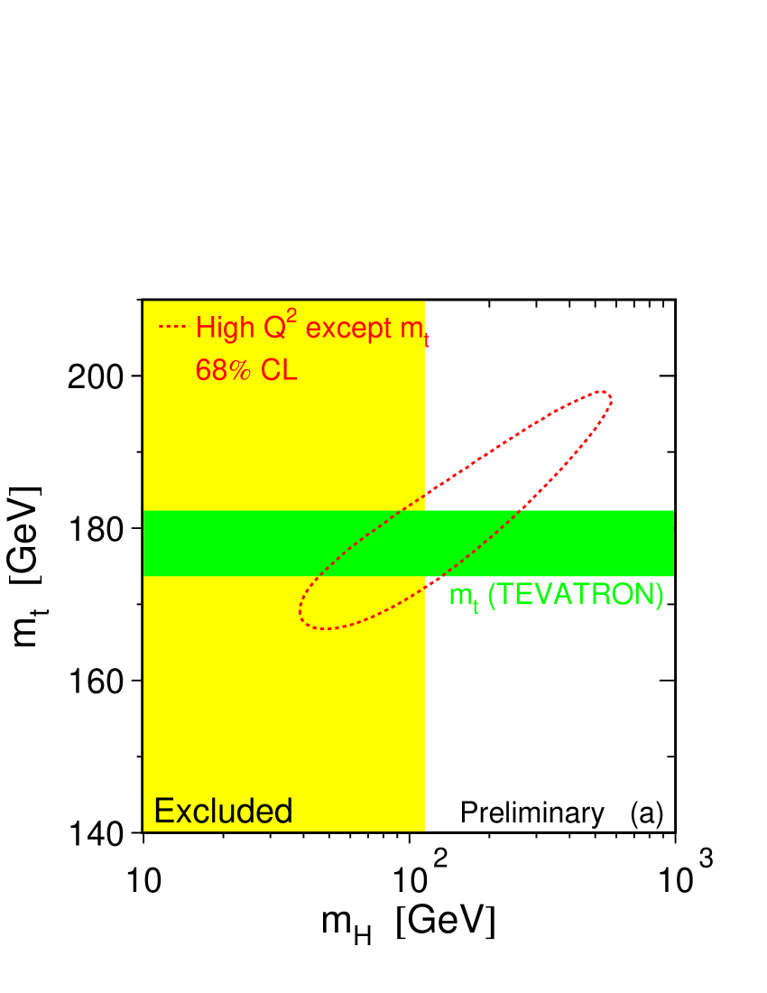
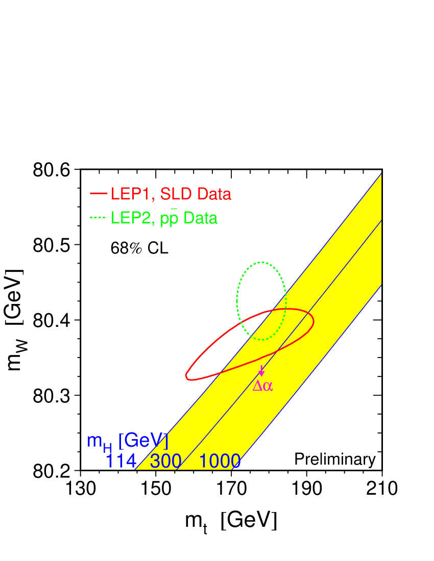
Figure 2: Results of fits to electroweak data [47]. Direct Higgs boson searches at LEP2 and the top mass measurement at the Tevatron are summarised in these plots. (a) shows the plane “top mass versus Higgs mass”. The light shaded area is excluded by direct searches for the Higgs boson at LEP2. The dark shaded area is given by the central value of the direct top mass measurement at the Tevatron and its errors. The dashed line encloses the region preferred by the electroweak data at 68% confidence level. (b) shows the “$M_{W}$ versus $M_{\mathrm{top}}$” plane. The full line encloses the area preferred by the SM fit to data from LEP1 and SLD. The dashed contour indicates the result of the LEP2, UA2 and Tevatron $W$ mass measurements and the direct top quark mass measurement. The plot also shows the SM relationship of the masses as function of the Higgs boson mass.

Figure 3: Examples of loop diagrams of the $W$ propagator introducing a dependence of the $W$ mass on the top and Higgs mass.

As becomes clear from figure 2 increasing the precision of the direct measurements of $M_{W}$ and $M_{\mathrm{top}}$ is a precondition to gain higher leverage for SM predictions of the Higgs mass.

Summarising this section on electroweak precision measurements we point out two major issues with respect to the top quark. First, the very good agreement of the predicted value for $M_{\mathrm{top}}$ based on higher order electroweak corrections with the direct measurement is a significant success of the SM. Second, more precise measurements of $M_{\mathrm{top}}$ and $M_{W}$ are needed to obtain tighter constraints on the Higgs boson mass. This is one of the major physics motivations for the Run II of the Tevatron.

2.4 The top quark in flavour physics

Flavour physics describes the transitions between quarks of different flavour. These transitions always involve the exchange of a W boson. They are charged current interactions. Higher order transitions of this kind involve loops in which particles can occur that are much heavier than the hadrons involved in the interaction. Diagrams with down-type quarks ($d$, $s$ and $b$) in the loops cancel each other via the GIM mechanism very effectively, since they are nearly degenerate in their masses. The large degree of mass splitting in the up-quark sector prevents the cancellation and leads to sizeable loop contributions, e.g. in radiative $B$ meson decays. One other example where the top quark plays a prominent rôle is the mixing of neutral $B$ mesons.

The phenomenon of particle-antiparticle mixing has been experimentally established in the neutral kaon system ($K^{0}$–$\overline{K^{0}}$) and the $B^{0}_{d}$–$\overline{B^{0}_{d}}$ system [51, 52]. Mixing is also expected to take place in the $D^{0}$–$\overline{D^{0}}$ and $B^{0}_{s}$–$\overline{B^{0}_{s}}$ system, but was not observed yet. Only limits were set [53, 54, 55, 56, 57, 58, 59, 60, 61].

Mixing changes the flavour quantum number (strange, charm, bottom) of the mesons by two units ($\Delta S=2$, $\Delta C=2$, $\Delta B=2$). A neutral meson is produced in a well defined flavour eigenstate $|P^{0}\rangle$ or $|\overline{P^{0}}\rangle$ with $P\in\{K,D,B_{d},B_{s}\}$. This initial state evolves due to second order weak interactions into a time-dependent quantum superposition of the two flavour eigenstates: $|P(t)\rangle=a(t)\;|P^{0}\rangle+b(t)\;|\overline{P^{0}}\rangle$. The time-evolution of the coefficients $a(t)$ and $b(t)$ is given by the effective Hamiltonian matrix $\mathbf{H}=\mathbf{M}-\rmi/2\;\mathbf{\Gamma}\$:

$$\rmi\ \frac{\partial}{\partial t}\ \left(\begin{array}[]{c}a(t)\\ b(t)\end{array}\right)=\left(\mathbf{M}-\frac{\rmi}{2}\;\mathbf{\Gamma}\right)\ \left(\begin{array}[]{c}a(t)\\ b(t)\end{array}\right)$$ (14)

$\mathbf{M}$ and $\mathbf{\Gamma}$ are $2\times 2$ Hermitian matrices denoted as mass and decay matrix, respectively. CPT invariance requires $M_{11}=M_{22}=M$ and $\Gamma_{11}=\Gamma_{22}=\Gamma$, where M and $\Gamma$ are the mass and the decay width of the flavour eigenstates.

In case of the B meson systems ($B^{0}_{d}$–$\overline{B^{0}_{d}}$ and $B^{0}_{s}$–$\overline{B^{0}_{s}}$) the transition amplitude for the mixing matrix is dominated by box diagrams involving the top quark, see figure 4.

Figure 4: Lowest order Feynman diagrams for B meson mixing. A $\overline{B^{0}}\;(b\bar{d})$ or a $\overline{B^{0}_{s}}\;(b\bar{s})$ oscillates into a $B^{0}\;(\bar{b}d)$ or a $B^{0}_{s}\;(\bar{b}s)$, respectively.

All up-type quarks ($q=u,c,t$) can be exchanged in the box and contribute in general to the mixing amplitude. In the case of $B$ mesons it is, however, found that the mixing is strongly dominated by the diagrams with two top quarks in the loop as shown in figure 4. All other diagrams involving at least one u- or c-quark can be neglected with respect to the top-top diagram [62, 63, 64]. As a side remark: In the neutral kaon system the case is different. Charm and top quark box diagrams as well as intermediate virtual pion states contribute significantly to the mixing. For $B$ mixing the off-diagonal elements of $\mathbf{M}$ and $\mathbf{\Gamma}$, $\langle B^{0}_{q}|H_{\mathit{eff}}^{\Delta B=2}|\overline{B^{0}_{q}}\rangle=M_{12}-i/2\;\Gamma_{12}$ ($q\in\{d,s\}$), are in very good approximation given by [62, 64, 10]:

$$M_{12,q} = -\frac{G_{F}^{2}M^{2}_{W}}{12\;\pi^{2}}\ m_{B_{q}}f^{2}_{B_{q}}B_{B_{q}}\eta_{B}\cdot\left(V^{*}_{tq}\,V_{tb}\right)^{2}\cdot S_{0}(x_{t})$$ (15)

$$\Gamma_{12,q} = \frac{G_{F}^{2}}{8\;\pi}\ m_{b}^{2}m_{B_{q}}f^{2}_{B_{q}}B_{B_{q}}\eta^{\prime}_{B}\cdot\left[\left(V^{*}_{tq}V_{tb}\right)^{2}+V^{*}_{tq}V_{tb}V^{*}_{cq}V_{cb}\ \mathcal{O}\left(\frac{m_{c}^{2}}{m_{b}^{2}}\right)+\right.$$ (16)

$$\left.\left(V_{cq}^{*}V_{cb}\right)^{2}\ \mathcal{O}\left(\frac{m_{c}^{4}}{m_{b}^{4}}\right)\right]$$

where $G_{F}$ is the Fermi constant and $M_{W}$ the W mass. $m_{b}$ and $m_{c}$ are the $b$ quark and $c$ quark masses, respectively. $m_{B_{q}}$ represents the masses of the $B_{d}^{0}$ and $B^{0}_{s}$ mesons. $f_{B_{q}}$ is the decay constant and $B_{B_{q}}$ the bag parameter introduced as a correction factor to hadronic matrix elements. The $V_{ij}$ are the CKM matrix elements. $x_{t}=(M_{\mathrm{top}}/M_{W})^{2}$ is the squared ratio of top quark mass over W mass. The function $S_{0}(x_{t})$ is an Inami-Lim function [65] and can be well approximated by $S_{0}(x_{t})=0.784\;x_{t}^{0.76}$ [66]. The parameters $\eta_{B}$ and $\eta^{\prime}_{B}$ represent QCD corrections to the box diagram. The mass eigenstates $B_{h}$ (h for heavy) and $B_{l}$ (l for light) diagonalize the effective Hamiltonian $H$ and are given by: $|B_{h}\rangle=p\,|B^{0}\rangle-q\,|\overline{B^{0}}\rangle$ and $|B_{l}\rangle=p\,|B^{0}\rangle+q\,|\overline{B^{0}}\rangle$ with $q^{2}=M_{12}^{*}-\rmi/2\,\Gamma^{*}_{12}$ and $p^{2}=M_{12}-\rmi/2\,\Gamma^{*}_{12}$. Mixing experiments do not determine the masses $m_{h}$ and $m_{l}$ but rather the mass difference between the two $\Delta m=m_{h}-m_{l}$ which is in good approximation (about 1% accuracy) theoretically predicted to be $\Delta m=2\,|M_{12}|$ [64]. This quantity depends on the top quark mass via $\eta_{B}S_{0}(x_{t})$. To give a flavour of the dependency: $\eta_{B}S_{0}(x_{t})$ changes from roughly 1.1 for $M_{\mathrm{top}}=150$ GeV to 1.7 at $M_{\mathrm{top}}=200$ GeV [67]. Historically, the ARGUS measurement of $B^{0}_{d}$–$\overline{B^{0}_{d}}$ mixing yielded a mass difference $\Delta m_{d}$ found to be surprisingly large [52]. Using the dependence of $\Delta m_{d}$ on the top quark mass several authors interpreted this measurement as a hint of a large top quark mass [68, 69, 70, 71, 72].

The dependence on $M_{\mathrm{top}}$ drops out if the ratio

$$\frac{\Delta m_{s}}{\Delta m_{d}}=\frac{m_{B_{s}}f^{2}_{B_{s}}B_{B_{s}}}{m_{B_{d}}f^{2}_{B_{d}}B_{B_{d}}}\cdot\left|\frac{V_{ts}}{V_{td}}\right|^{2}$$ (17)

is taken. Once $\Delta m_{s}$ is measured in $B_{s}$ mixing this relation will allow to extract the absolute value of the ratio $V_{ts}/V_{td}$ with good precision.

3 Top quark production at hadron colliders

In this chapter we present the phenomenology of top quark production at hadron colliders. We limit the discussion to SM processes. Anomalous top quark production and non-SM decays will be covered in chapter 9. Specific theoretical cross section predictions refer to the Fermilab Tevatron, running at $\sqrt{s}=1.8\;\mathrm{TeV}$ (Run I) or $\sqrt{s}=1.96\;\mathrm{TeV}$ (Run II), or to the future Large Hadron Collider (LHC) at CERN ($\sqrt{s}=14\;\mathrm{TeV}$). In the intermediate future the Tevatron and the LHC are the only two colliders where SM top quark production can be observed.

The two basic production modes of top quarks at hadron colliders are the production of $t\bar{t}$ pairs, which is dominated by the strong interaction, and the production of single top quarks due to electroweak interactions.

3.1 $t\bar{t}$ production

We discuss only top quark pair production via the strong interaction. $t\bar{t}$ pairs can also be produced by electroweak interactions if a $Z^{0}$ or a photon are exchanged between the in- and outgoing quarks. However, at a hadron collider the cross sections for theses processes are completely negligible compared to the QCD cross section. The cross section for the pair production of heavy quarks has been calculated in perturbative QCD, i.e. as a perturbation series in the QCD running coupling constant $\alpha_{s}(\mu^{2})$. The results are applicable to the bottom and to the top quark. In the following we will refer only to $t\bar{t}$ production, the scope of this article.

3.1.1 The factorization ansatz

The underlying theoretical framework of the calculation is the parton model which regards a high-energy hadron $A$, in our case a proton or antiproton, as a composition of quasi-free partons (quarks and gluons) which share the longitudinal hadron momentum $p_{A}$. The parton $i$ has the longitudinal momentum $p_{i}$, i.e. it carries the momentum fraction $x_{i}=p_{i}/p_{A}$. The cross section calculation is based on the factorization theorem stating that the cross section is given by the convolution of parton distribution functions (PDF) $f_{i}(x,\mu^{2})$ for the colliding hadrons ($A$, $B$) and the hard parton-parton cross section $\hat{\sigma}_{ij}$:

$$\sigma(AB\rightarrow t\bar{t})=\sum_{i,j}\int\,\rmd x_{i}\rmd x_{j}\;f_{i,A}(x_{i},\mu^{2})f_{j,B}(x_{j},\mu^{2})\cdot\hat{\sigma}_{ij}(ij\rightarrow t\bar{t};\hat{s},\mu^{2})$$ (18)

The hadrons $AB$ are either $p\bar{p}$ (at the Tevatron) or $pp$ (at the LHC). The parton distribution function $f_{i,A}(x_{i},\mu^{2})$ describes the probability density for finding a parton $i$ inside the hadron $A$ carrying a longitudinal momentum fraction $x_{i}$.

The parton distribution functions and the parton-parton cross section $\hat{\sigma}_{ij}$ depend on the factorization and renormalization scale $\mu$. For calculating heavy quark production the scale is usually set to be of the order of the heavy quark mass, here specifically $\mu=M_{\mathrm{top}}$. Strictly speaking one has to distinguish between the factorization scale $\mu_{F}$ introduced by the factorization ansatz and the renormalization scale $\mu_{R}$ due to the renormalization procedure invoked to regulate divergent terms in the perturbation series when calculating the parton-parton cross section $\hat{\sigma}_{ij}$. Since both scales are to some extent arbitrary parameters most authors have adopted the practice to use only one scale $\mu=\mu_{F}=\mu_{R}$ in their calculations. If the complete perturbation series could be calculated, the result for the cross section would be independent of $\mu$. However, since calculations are performed at finite order in perturbation theory, cross section predictions do in general depend on the choice of $\mu$. The $\mu$-dependence is usually tested by varying the scale between $\mu=M_{\mathrm{top}}/2$ and $\mu=2\,M_{\mathrm{top}}$. The variations in the cross section are quoted as an indicative theoretical uncertainty of the prediction, but should not be mistaken for Gaussian errors.

In (18) the variable $\hat{s}$ denotes the square of the centre-of-mass energy of the colliding partons: $\hat{s}=x_{i}x_{j}(p_{A}+p_{B})^{2}$. In symmetric colliders, where $p_{A}=p_{B}=p$, we have $\hat{s}=4\,x_{i}x_{j}p^{2}=x_{i}x_{j}s$. The sum in (18) runs over all pairs of light partons $(i,j)$ contributing to the process. The factorization scheme serves as a method to systematically eliminate collinear divergencies from the parton cross section $\hat{\sigma}_{ij}$ and absorb them into the parton distribution functions. A detailed theoretical justification for the applicability of the factorization ansatz to heavy quark production can be found in reference [73]. According to this analysis effects such as an intrinsic heavy quark component in the hadron wave function and flavour excitation processes like $qt\rightarrow qt$ do not lead to a breakdown of the conventional factorization formula.

3.1.2 Parametrizations of parton distribution functions

The PDFs are extracted from measurements in deep inelastic scattering experiments where either electrons, positrons or neutrinos collide with nucleons. A variety of experiments of this kind have been conducted since the late 1960s and provided hard evidence for the parton (quark) model in the first place. During the 1990s the experiments ZEUS and H1 [74] at the $ep$ storage ring HERA at DESY have reached an outstanding precision in measurements of the proton structure, which meant a big leap forward for the prediction of cross sections at hadron colliders.

Several parametrizations of proton PDFs have been extracted from the experimental data by different groups of physicists. As an example figure 5 shows PDFs of the CTEQ3M parametrization [75].

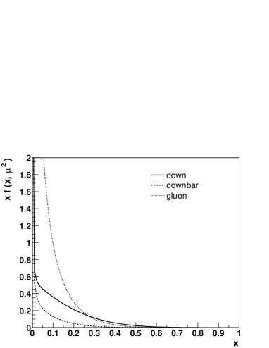
Figure 5: Parton distribution functions (PDFs) of $u$ quarks, $\bar{u}$ quarks, $d$ quarks, $\bar{d}$ quarks and gluons inside the proton. The parametrization is CTEQ3M [75]. The scale at which the PDFs are evaluated was chosen to be $\mu=175\;\mathrm{GeV}$ ($\mu^{2}=30625\;\mathrm{GeV^{2}}$).

Plotted are the distributions most relevant for $p\bar{p}$ and $pp$ collisions, the PDFs for $u$, $\bar{u}$, $d$, $\bar{d}$ and the gluons. For antiprotons the distributions in figure 5 have to be reversed between quark and antiquark. The scale $\mu$ was chosen to be $\mu=175\;\mathrm{GeV}$. One sees that the gluons start to dominate in the $x$ region below 0.15. The $t\bar{t}$ production cross section at the Tevatron is dominated by the large $x$ region, since the top quark mass is relatively large compared to the Tevatron beam energy ($M_{\mathrm{top}}/\sqrt{s}=0.0875$). At the LHC ($M_{\mathrm{top}}/\sqrt{s}=0.0125$) the lower x region becomes more important.

There are differences between the various sets of PDF parametrizations. To give the reader a quantitative impression we compare the CTEQ3M, MRSR2 and MRSD parametrizations in figure 6.

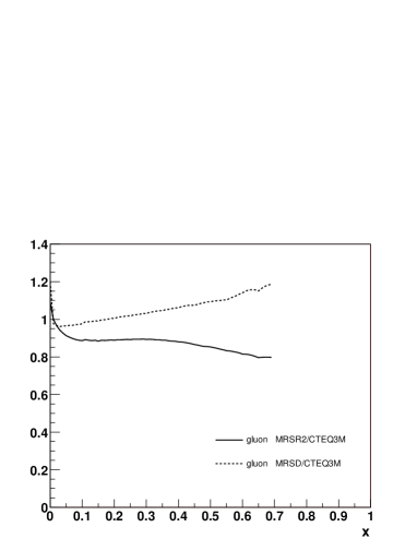
Figure 6: Comparison of the CTEQ3M, MRSR2 and MRSD parametrizations for the PDF of the up quark and the gluon. The left plot shows the ratios $f_{u}(x)_{\mathrm{MRSR2}}/f_{u}(x)_{\mathrm{CTEQ3M}}$ (full line) and $f_{u}(x)_{\mathrm{MRSD}}/f_{u}(x)_{\mathrm{CTEQ3M}}$ (dashed line). On the right hand side we plot $f_{g}(x)_{\mathrm{MRSR2}}/f_{g}(x)_{\mathrm{CTEQ3M}}$ (full line) and $f_{g}(x)_{\mathrm{MRSD}}/f_{g}(x)_{\mathrm{CTEQ3M}}$ (dashed line). The factorization scale is set to $\mu^{2}=30625\;\mathrm{GeV^{2}}$.

As a representative example we plot the ratios $f_{u}(x)_{\mathrm{MRSR2}}/f_{u}(x)_{\mathrm{CTEQ3M}}$ and $f_{u}(x)_{\mathrm{MRSD}}/f_{u}(x)_{\mathrm{CTEQ3M}}$ for up-quarks as well as $f_{g}(x)_{\mathrm{MRSR2}}/f_{g}(x)_{\mathrm{CTEQ3M}}$ and $f_{g}(x)_{\mathrm{MRSD}}/f_{g}(x)_{\mathrm{CTEQ3M}}$ for gluons. These three PDF parametrizations were chosen because they are used for predictions of the $t\bar{t}$ cross section at the Tevatron [76, 77, 78]. Typical differences are on the order of 5 to 10%.

3.1.3 The parton cross section

The cross section $\hat{\sigma}$ of the hard, i.e. short distance, parton-parton process $ij\rightarrow t\bar{t}$ can be calculated in perturbative QCD. The leading order processes, contributing with $\alpha_{s}^{2}$ to the perturbation series, are quark-antiquark annihilation, $q\bar{q}\rightarrow t\bar{t}$, and gluon fusion, $gg\rightarrow t\bar{t}$. The corresponding Feynman diagrams for these processes are depicted in figure 7.

Figure 7: Feynman diagrams of the leading order processes for $t\bar{t}$ production: quark-antiquark annihilation ($q\bar{q}\rightarrow t\bar{t}$) and gluon fusion ($gg\rightarrow t\bar{t}$).

The leading order (Born) cross sections for heavy quark production were calculated in the late 1970s [79, 80, 81, 82, 83, 84], most of them having charm production as a concrete application in mind. The differential cross section for quark-antiquark annihilation is given by

$$\frac{\rmd\hat{\sigma}}{\rmd\hat{t}}\left(q\bar{q}\rightarrow t\bar{t}\right)=\frac{4\,\pi\,\alpha_{s}^{2}}{9\,\hat{s}^{4}}\cdot\left[(m^{2}-\hat{t})^{2}+(m^{2}-\hat{u})^{2}+2m^{2}\hat{s}\right]$$ (19)

where $\hat{s}$, $\hat{t}$ and $\hat{u}$ are the Lorentz-invariant Mandelstam variables of the process. They are defined by $\hat{s}=(p_{q}+p_{\,\bar{q}})^{2}$, $\hat{t}=(p_{q}-p_{t})^{2}$ and $\hat{u}=(p_{q}-p_{\,\bar{t}})^{2}$ with $p_{i}$ being the corresponding momentum 4-vector of the quark $i$. $m$ denotes the top quark mass. The differential cross section for the gluon-gluon fusion process is given by:

$$\frac{\rmd\hat{\sigma}}{\rmd\hat{t}}\left(g_{1}g_{2}\rightarrow t\bar{t}\right) = \frac{\pi\,\alpha_{s}^{2}}{8\,\hat{s}^{2}}\cdot\left[\frac{6(m^{2}-\hat{t})(m^{2}-\hat{u})}{\hat{s}^{2}}-\frac{m^{2}(\hat{s}-4\,m^{2})}{3\,(m^{2}-\hat{t})(m^{2}-\hat{u})}\right.$$ (20)

$$\left.+\frac{4}{3}\cdot\frac{(m^{2}-\hat{t})(m^{2}-\hat{u})-2\,m^{2}(m^{2}+\hat{t})}{(m^{2}-\hat{t})^{2}}+\frac{4}{3}\cdot\frac{(m^{2}-\hat{t})(m^{2}-\hat{u})-2\,m^{2}(m^{2}+\hat{u})}{(m^{2}-\hat{u})^{2}}\right.$$

$$\left.-3\cdot\frac{(m^{2}-\hat{t})(m^{2}-\hat{u})-m^{2}(\hat{u}-\hat{t})}{\hat{s}\,(m^{2}-\hat{t})^{2}}-3\cdot\frac{(m^{2}-\hat{t})(m^{2}-\hat{u})-m^{2}(\hat{t}-\hat{u})}{\hat{s}\,(m^{2}-\hat{u})^{2}}\right]$$

The invariant variables are in this case $\hat{s}=(p_{g1}+p_{g2})^{2}$, $\hat{t}=(p_{g1}-p_{t})^{2}$ and $\hat{u}=(p_{g1}-p_{\,\bar{t}})^{2}$. The cross sections in (19) and (20) are quoted in the form given in reference [11]. The invariants $\hat{t}$ and $\hat{u}$ may be expressed in terms of the cosine of the scattering angle $\hat{\theta}$ in the parton-parton centre-of-mass system:

$$\cos{\hat{\theta}}=\sqrt{1-\frac{4\,p_{\perp}^{2}}{\hat{s}}}\ \ \ \ \ \ \ \ \ \ \ \hat{t}=-\frac{\hat{s}}{2}(1-\cos{\hat{\theta}})\ \ \ \ \ \ \ \ \ \ \ \hat{u}=-\frac{\hat{s}}{2}(1+\cos{\hat{\theta}})$$ (21)

where $p_{\perp}$ is the common transverse momentum of the outgoing top quarks.

A full calculation of next-to-leading order (NLO) corrections contributing in order $\alpha_{s}^{3}$ to the inclusive parton-parton cross section for heavy quark pair production was performed independently by two groups: Nason et al. in 1988 [85] and Beenakker et al. in 1991 [86, 87], yielding consistent results. The NLO calculations involve virtual contributions to the leading order processes, gluon bremsstrahlung processes ($q\bar{q}\rightarrow t\bar{t}+g$ and $gg\rightarrow t\bar{t}+g$) as well as processes like $g+q(\bar{q})\rightarrow t\bar{t}+q(\bar{q})$. Examples of Feynman diagrams of NLO processes are given in figure 8:

(a)                         (b)                         (c)                         (d)

Figure 8: Example Feynman diagrams of next-to-leading order (NLO) corrections to quark-antiquark annihilation and gluon fusion. a) and c) show virtual corrections, b) and d) gluon bremsstrahlung graphs.

a) and c) display two virtual graphs, b) and d) two gluon bremsstrahlung graphs. $\alpha^{3}_{s}$ corrections arise when interfering those graphs with the leading order graphs of figure 7. For the NLO calculation of the hadron-hadron cross section $\sigma(AB\rightarrow t\bar{t})$ to be consistent one has to use next-to-leading order determinations of the coupling constant $\alpha_{s}$ and the PDFs. All quantities have to be consistently defined in the same renormalization scheme because different approaches distribute the radiative corrections differently among the parton-parton cross section, the PDFs and $\alpha_{s}$. Most authors use the $\mathrm{\overline{MS}}$ or an extension of the $\mathrm{\overline{MS}}$ scheme. First NLO cross section predictions for $t\bar{t}$ production at the Tevatron ($\sqrt{s}=1.8\;\mathrm{TeV}$) yielded values of about 4 pb [88, 87, 89, 90]

At energies close to the kinematic threshold, $\hat{s}=4\,M_{\mathrm{top}}^{2}$, the quark-antiquark annihilation process is the dominant one, if the incoming quarks are valence quarks, as is the case of $p\bar{p}$ collisions. At the Tevatron 80 to 90% of the $t\bar{t}$ cross section is due to quark-antiquark annihilation [78, 77, 91]. At higher energies the gluon-gluon fusion process dominates for both $p\bar{p}$ and $pp$ collisions. That is why one can built the LHC as a $pp$ machine without compromising the parton-parton cross section. Technically, it is of course much easier to operate a $pp$ collider, since one spares the major challenge to produce high antiproton currents in a storage ring. For the Tevatron the ratio of NLO over LO cross sections for gluon-gluon fusion is predicted to be 1.8 at $M_{\mathrm{top}}=175\;\mathrm{GeV}/c^{2}$, for quark-antiquark annihilation the value is only about 1.2 [78]. Since the annihilation process is dominating, the overall NLO enhancement is about 1.25.

3.1.4 Soft gluon resummation

Contributions to the total cross section due to radiative corrections are large in the region near threshold ($\hat{s}=4\,M_{\mathrm{top}}^{2}$) and at high energies ($\hat{s}>400\;M_{\mathrm{top}}^{2}$). Near threshold the cross section is enhanced due to initial state gluon bremsstrahlung (ISGB) [92]. This effect is important for $t\bar{t}$ production at the Tevatron, but not for the LHC where gluon splitting and flavour excitation are increasingly important effects. The calculation at fixed next-to-leading order ($\alpha_{s}^{3}$) perturbation theory has been refined to systematically incorporate higher order corrections due to soft gluon radiation. Technically, this is done by applying an integral transform (Mellin transform) to the cross section:

$$\sigma_{N}(t\bar{t})\equiv\int_{0}^{1}\rmd\rho\ \rho^{N-1}\;\sigma(\rho;t\bar{t})$$ (22)

where $\rho=4\,M_{\mathrm{top}}^{2}/s$ is a dimensionless parameter. In Mellin moment space the corrections due to soft gluon radiation are given by a power series of logarithms $\ln N$. For $\mu=M_{\mathrm{top}}$ the corrections are positive at all orders. Therefore, the resummation of the soft gluon logarithms yields an increase of the $t\bar{t}$ cross section with respect to the NLO value. Four different groups have presented cross section predictions based on the resummation of soft gluon contributions: (1) Laenen et al. [92, 78], (2) Berger and Contopanagos [93, 94, 76], (3) Bonciani et al. (BCMN) [95, 96, 77, 91] and (4) Kidonakis et al. [97, 98, 99]. Their predictions for $M_{\mathrm{top}}=175\;\mathrm{GeV}/c^{2}$ are summarised in table 3.

Table 3: Cross section predictions for $t\bar{t}$ production at next-to-leading order (NLO) in perturbation theory including the resummation of initial state gluon bremsstrahlung (ISGB). The predictions are given for a top mass of $M_{\mathrm{top}}=175\;\mathrm{GeV}/c^{2}$. The cross sections are given for $p\bar{p}$ collisions at the Tevatron ($\sqrt{s}=1.8\;\mathrm{TeV}$ and $\sqrt{s}=1.96\;\mathrm{TeV}$) and $pp$ collisions at the LHC ($\sqrt{s}=14\;\mathrm{TeV}$). The factorization and renormalization scale is set to $\mu=M_{\mathrm{top}}$ to derive the central values. It has to be stressed that the authors use different sets of PDF parametrizations. Part of the differences can be attributed to this fact. In reference [78] Laenen et al. do not provide a direct prediction for $M_{\mathrm{top}}=175\;\mathrm{GeV}/c^{2}$. To compare their prediction with those of other authors I choose to linearly interpolate the given values for $M_{\mathrm{top}}=174\;\mathrm{GeV}/c^{2}$ and $M_{\mathrm{top}}=176\;\mathrm{GeV}/c^{2}$, thereby neglecting the functional form of the mass dependence. Within the assigned errors this simplification is acceptable.

Group	$\sqrt{s}$	PDF set	$\sigma(t\bar{t})$	Reference
(1) Laenen at al.	1.8 TeV	MRSD_’	$4.95^{+0.70}_{-0.42}$ pb	[78]
(2) Berger and Contopanagos	1.8 TeV	CTEQ3M	$5.52^{+0.07}_{-0.45}$ pb	[93, 94, 76]
(3) Bonciani et al.	1.8 TeV	CTEQ6M	$5.19^{+0.52}_{-0.68}$ pb	[91]
(4) Kidonakis et al.	1.8 TeV	MRST2002	$(5.24\pm 0.31)$ pb	[99]
(2) Berger and Contopanagos	2.0 TeV	CTEQ3M	$7.56^{+0.10}_{-0.55}$ pb	[94, 76]
(3) Bonciani et al.	1.96 TeV	CTEQ6M	$6.70^{+0.71}_{-0.88}$ pb	[91]
(4) Kidonakis et al.	1.96 TeV	MRST2002	$(6.77\pm 0.42)$ pb	[99]
(2) Berger and Contopanagos	14.0 TeV	CTEQ3M	760 pb	[94, 76]
(3) Bonciani et al.	14.0 TeV	MRSR2	$833^{+52}_{-39}$ pb	[77]
(4) Kidonakis et al.	14.0 TeV	MRST2002	870 pb	[99]

In the region very close to the kinematic threshold non-perturbative effects become dominant and the perturbative approach breaks down. The resummation can therefore not sensibly be extended into this region. That is why Laenen et al. introduce a new scale $\mu_{0}$ with $\Lambda_{\mathrm{QCD}}\ll\mu_{0}\ll M_{\mathrm{top}}$ where they stop the resummation. The concrete choice of scale is to some extent arbitrary. The uncertainty quoted by Laenen et al. is derived by varying the scale $\mu_{0}$. To calculate the central value of the cross section they use $\mu_{0}=0.1\,M_{\mathrm{top}}$ for $q\bar{q}$-annihilation and $\mu_{0}=0.25\,M_{\mathrm{top}}$ for $gg$-fusion. The values are not required to be the same, since the respective perturbation series have different convergence properties.

Berger and Contopanagos derive the infra-red cut-off $\mu_{0}$ within their calculation and thereby define a perturbative region where resummation can be applied. Since $\mu_{0}$ is derived, it is not treated as a source of error in this approach. The theoretical uncertainty quoted by Berger and Contopanagos is derived by varying the factorization and renormalization scale $\mu$ between $0.5\,M_{\mathrm{top}}$ and $2\,M_{\mathrm{top}}$. The central value, given in table 3, is calculated using the CTEQ3M PDFs. The uncertainty due to the choice of the PDF parametrization is about 4%. Resummation effects are of appreciable size: The resummed total cross sections (for $\sqrt{s}=1.8\;\mathrm{TeV}$ and $\sqrt{s}=2.0\;\mathrm{TeV}$, respectively) are about 9% above the NLO cross sections. Berger and Contopanagos predict an increase of 37% in cross section, when going from $\sqrt{s}=1.8\;\mathrm{TeV}$ to $\sqrt{s}=2.0\;\mathrm{TeV}$ in Run II of the Tevatron. The cross section value for the LHC, $\sigma=760\;\mathrm{pb}$, merely reflects an estimate and is not accompanied by an uncertainty. Due to the much larger centre-of-mass energy at the LHC the near threshold region is much less important for $t\bar{t}$ production, reducing the significance of ISGB and the need for resummation of these contributions.

While the first two groups have only resummed leading logarithmic terms (LL), BCMN also include next-to-leading logarithms (NLL). They used a different resummation prescription which does not demand the introduction of an additional infra-red cut-off $\mu_{0}$ [95]. The LL result of BCMN shows only an increase of about 1% compared to the NLO cross section at the Tevatron [96]. When taking NLL terms into account the increase is 4% [77]. In table 3 we quote the NLL results as updated in reference [91] with the newest set of PDFs. The errors quoted by BCMN include PDF uncertainties, which are evaluated by using sets of PDF parametrizations that provide an estimate of “1-$\sigma$” uncertainties. In the case of CTEQ [100, 101] 40 different sets are available, for MRST [102] there are 30 sets. Kidonakis et al. resum leading and subleading logarithms up to order $\alpha_{s}^{4}$ in an attempt to reduce the dependence of the cross-section on the renormalization scale $\mu$ compared to the NLO calculation. The uncertainty quoted by Kidonakis et al. is dominated by the choice of the kinematic description of the scattering process, either in one-particle-inclusive or pair-invariant-mass kinematics. The Tevatron predictions given in table 3 are the average of the two choices. The LHC prediction is based on the one-particle-inclusive value, since this is believed to be more appropriate when the cross section is dominated by gluon-gluon fusion.

The cross section predictions are strongly dependent on the top quark mass, which is illustrated in figure 9.

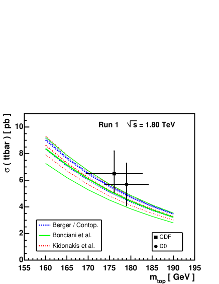
Figure 9: The $t\bar{t}$ cross section at $\sqrt{s}=1.8\;\mathrm{TeV}$ as a function of the top quark mass. The thick full line represents the central value predicted by Catani et al. [96, 77]. The thick dashed line shows the prediction by Berger and Contopanagos [94]. The thick dashed-dotted line is the prediction by Kidonakis et al. [99]. The thin lines indicate the upper and lower uncertainties of the predictions. The Run I measurements of CDF [103, 104] and DØ  [105, 106] are shown for comparison.

The plot shows the predictions for the Tevatron at $\sqrt{s}=1.8\;\mathrm{TeV}$, they are in good agreement within the given errors. For comparison the Run I measurements of CDF [103, 104] and DØ [105, 106] are shown. Within the large errors the measurements agree well with the theoretical predictions. It is obvious that a precise cross section measurement has to be accompanied by a precise measurement of the top quark mass to provide a basis for a stringent test of the theory.

3.2 Single top quark production

Top quarks can be produced singly via electroweak interactions involving the $Wtb$ vertex. There are three production modes which are distinguished by the virtuality $Q^{2}$ of the $W$ boson ($Q^{2}=-q^{2}$, where $q$ is the four-momentum of the $W$):

1. the t-channel ($q^{2}=\hat{t}\;$): A virtual W strikes a $b$ quark (a sea quark) inside the proton. The W boson is spacelike ($q^{2}<0$). This mode is also known as W-gluon fusion, since the $b$ quark originates from a gluon splitting into a $b\overline{b}$ pair. Feynman diagrams representing this process are shown in figure 10a and figure 10b . $W$-gluon fusion is the dominant production mode, both at the Tevatron and at the LHC, as will be shown in the discussion below.

2. the s-channel ($q^{2}=\hat{s}\;$): This production mode is of Drell-Yan type. A timelike $W$ boson with $q^{2}\geq(M_{\mathrm{top}}+m_{b})^{2}$ is produced by the fusion of two quarks belonging to an SU(2) isospin doublet. See figure 10c for the Feynman diagram.

3. associated production: The top quark is produced in association with a real (or close to real) $W$ boson ($q^{2}=M_{W}^{2}$). The initial $b$ quark is a sea quark inside the proton. Figure 10d shows the Feynman diagram. The cross section is negligible at the Tevatron, but of considerable size at LHC energies where associated production even supercedes the $s$-channel.

(a)                            (b)                              (c)                         (d)

Figure 10: Representative Feynman diagrams for the three single top production modes. a) and b) show $W$-gluon fusion graphs, c) the $s$-channel process and d) associated production. We chose to draw the graphs in a), b) and c) with the $(u,d)$ weak-isospin doublet coupling to the $W$. This is by far the dominating contribution. In general, also the $(c,s)$ doublet contributes. The graphs show single top quark production, the diagrams for single antitop quark production can be obtained by interchanging quarks and antiquarks.

In $p\bar{p}$ and $pp$ collisions the cross section is dominated by contributions from up and down quarks coupling to the $W$ boson on one hand side of the Feynman diagrams. That is why the $(u,d\,)$ quark doublet is shown in the graphs of figure 10. There is of course also a small contribution from the second weak isospin quark doublet, $(c,s)$; an effect of about 2% for $s$- and 6% for $t$-channel production [107]. Furthermore, we will only consider single top quark production via a $Wtb$ vertex. The production channels involving a $Wtd$ or a $Wts$ vertex are strongly suppressed due to small CKM matrix elements: $0.0048<|V_{td}|<0.014$ and $0.037<|V_{ts}|<0.043$ [10]. Thus, their contribution to the total cross section is quite small: $\sim 0.1\%$ and $\sim 1\%$, respectively [108]. In the following paragraphs we will review the theoretical cross section predictions for the three single top processes and the methods with which they are obtained.

3.2.1 W-gluon fusion

The $W$-gluon fusion process was already suggested as a potentially interesting source of top quarks in the mid 1980s [109, 110] and early 1990s [111]. If the $b$ quark is taken to be massless, a singularity arises when computing the diagram in figure 10a in case the final $\bar{b}$ quark is collinear with the incoming gluon. In reality the non-zero mass of the $b$ quark regulates this collinear divergence. When calculating the total cross section the collinear singularity manifests itself as terms proportional to $\ln((Q^{2}+M_{\mathrm{top}}^{2})/m_{b}^{2})$ with $Q^{2}=-q^{2}$ being the virtuality of the W boson. These logarithmic terms cause the perturbation series to converge rather slowly. This difficulty can be obviated by introducing a parton distribution function (PDF) for the $b$ quark, $b(x,\mu^{2})$, which effectively resums the logarithms to all orders of perturbation theory and implicitly describes the splitting of gluons into $b\bar{b}$ pairs inside the colliding hadrons [112, 113]. Once a $b$ quark distribution function is introduced into the calculation, the leading order process is $q_{i}+b\rightarrow q_{j}+t$ as shown in figure11a.

(a)                                     (b)                                   (c)

Figure 11: a) shows the leading order Feynman diagram for $W$ gluon fusion if the perturbative calculation is performed involving a $b$ quark distribution function. b) and c) show two examples of $\alpha_{s}$ corrections to the leading order diagram. b) is a correction to the $b$ vertex, c) a correction to the light quark vertex.

In this formalism the process shown in figure 10a is a higher order correction which is already partially included in the b-quark distribution function. The remaining contribution is of order $1/\ln((Q^{2}+M_{\mathrm{top}}^{2})/m_{b}^{2})$ with respect to the leading order process in figure 11a. Additionally, there are also corrections of order $\alpha_{s}$: Two examples of those are shown in figure 11b and figure 11c. The leading order differential cross section calculated from the Feynman graph in figure 11a for quark-quark or antiquark-antiquark collisions is given by [109]:

$$\frac{\rmd\hat{\sigma}_{ij}}{\rmd\hat{t}}=\frac{\pi\,\alpha_{w}^{2}}{4}\cdot|V_{ij}|^{2}\;|V_{tb}|^{2}\cdot\frac{\hat{s}-M_{\mathrm{top}}^{2}}{(\hat{s}-m_{b}^{2})\,(\hat{t}-M_{W}^{2})^{2}}$$ (23)

For quark-antiquark collisions the result is:

$$\frac{\rmd\hat{\sigma}_{ij}}{\rmd\hat{t}}=\frac{\pi\,\alpha_{w}^{2}}{4}\cdot|V_{ij}|^{2}\;|V_{tb}|^{2}\cdot\frac{\hat{u}-m_{b}^{2}}{(\hat{s}-m_{b}^{2})^{2}}\;\frac{\hat{u}-M_{\mathrm{top}}^{2}}{(\hat{t}-M_{W}^{2})^{2}}$$ (24)

$\alpha_{w}=g_{w}^{2}/(4\,\pi)$ is the weak fine structure constant. The Mandelstam variable $\hat{t}$ is given by

$$\hat{t}=-\frac{\hat{s}}{2}\left(1-\frac{m_{b}^{2}}{\hat{s}}\right)\left(1-\frac{M_{\mathrm{top}}^{2}}{\hat{s}}\right)\cdot(1-\cos\hat{\theta})$$ (25)

and $\hat{s}+\hat{t}+\hat{u}=m_{b}^{2}+M_{\mathrm{top}}^{2}$. Another leading order calculations of the cross section was done van der Heide et al. [114].

The NLO calculation at first order in $\alpha_{s}$ comprises the square of the Born terms, (23) and (24), plus the interference with the virtual graphs plus the square of the real graphs with one single QCD coupling, e.g. figure 11c. Bordes and van Eijk presented an NLO calculation based on the formalism described above in 1995 [112]. They predict an enhancement of +28% of the NLO cross section over the Born cross section for the Tevatron operating at $\sqrt{s}=1.8\;\mathrm{TeV}$. Bordes and van Eijk used small masses for gluons and quarks to regularize infrared and collinear divergencies. Mass factorization was performed in the deep inelastic scattering (DIS) scheme. Stelzer et al. [113, 115] performed an NLO calculation entirely based on the $\overline{MS}$ factorization scheme. They predict a decrease of the cross section when going from leading order to NLO by about -8% to -10%.

The latest calculation was done by Harris et al. in 2002 [116] and contains full differential information, such that experimental acceptance cuts and jet definitions can be applied. Their results are summarised in table 4. We quote only these latest results for the cross sections, since previous calculations used different PDFs, which by itself leads to big differences in the predicted values. Harris et al. compare their results with those given by Stelzer et al. using the latest PDFs. The agreement is very good, within 1%.

Table 4: Predicted total cross sections for single top quark production processes. The cross sections are given for $p\bar{p}$ collisions at the Tevatron ($\sqrt{s}=1.8\;\mathrm{TeV}$ or $\sqrt{s}=1.96\;\mathrm{TeV}$) and $pp$ collisions at the LHC ($\sqrt{s}=14\;\mathrm{TeV}$). The cross sections of the $t$- and $s$-channel process are taken from reference [116] and were evaluated with CTEQ5M1 PDFs. The uncertainties were evaluated in reference [117]. The values for associated production are taken from reference [118] (Tevatron at $\sqrt{s}=1.96\;\mathrm{TeV}$ and LHC) and reference. [107] (Tevatron at $\sqrt{s}=1.8\;\mathrm{TeV}$). All cross sections are given for a top quark mass of $M_{\mathrm{top}}=175\;\mathrm{GeV}/c^{2}$.

Process	$\sqrt{s}$	$\sigma(\mathrm{t-channel})$	$\sigma(\mathrm{s-channel})$	$\sigma(Wt)$
$p\bar{p}\rightarrow t/\bar{t}$	1.80 TeV	$1.45^{+0.20}_{-0.16}\;\mathrm{pb}$	$(0.75\pm 0.10)\;\mathrm{pb}$	$0.14^{+0.05}_{-0.02}\;\mathrm{pb}$
$p\bar{p}\rightarrow t/\bar{t}$	1.96 TeV	$1.98^{+0.28}_{-0.22}\;\mathrm{pb}$	$(0.88\pm 0.11)\;\mathrm{pb}$	$0.094^{+0.015}_{-0.012}\;\mathrm{pb}$
$pp\rightarrow t$	14.0 TeV	$(156\pm 8)\;\mathrm{pb}$	$(6.6\pm 0.6)\;\mathrm{pb}$	$14.0^{+3.8}_{-2.8}\;\mathrm{pb}$
$pp\rightarrow\bar{t}$	14.0 TeV	$(91\pm 5)\;\mathrm{pb}$	$(4.1\pm 0.4)\;\mathrm{pb}$	$14.0^{+3.8}_{-2.8}\;\mathrm{pb}$

The cross sections given for the Tevatron are the sum of top and antitop quark production. In $pp$ collisions at the LHC the $W$-gluon fusion cross section differs for top and antitop quark production, which are therefore treated separately in table 4. The increase in the centre-of-mass energy from 1.80 TeV to 1.96 TeV in Run II of the Tevatron is predicted to yield a 33% increase in the total cross section. The ratio of $\sigma_{Wg}/\sigma_{t\bar{t}}$ is about 30%, for the Tevatron as well as for the LHC. The uncertainties quoted in table 4 are evaluated in reference [117] and include the uncertainties due to the factorization scale $\mu$, the choice of PDF parameterization, and the uncertainty in the top quark mass. The factorization scale uncertainty is $\pm 4\%$ at the Tevatron and $\pm 3\%$ at the LHC. The central value was calculated with $\mu^{2}=Q^{2}+M_{\mathrm{top}}^{2}$ for the $b$ quark PDF. The scale for the light quark PDFs was set to $\mu^{2}=Q^{2}$.

Of course the $t$-channel single top cross section depends on the top quark mass. The current uncertainty in the top quark mass ($\Delta m=4.3\,\mathrm{GeV}/c^{2}$) corresponds to about 7% uncertainty in the cross section at the Tevatron and 3% at the LHC. The dependence is approximately linear in the relevant mass range.

At first glance it is astonishing that the cross section for $W$-gluon fusion is of the same order of magnitude as $t\bar{t}$ production although it is a weak interaction process. There are several issues that lead to this relative enhancement [109]:

1. The parton cross section of the $W$-gluon fusion mode scales like $1/M_{W}^{2}$ as opposed to the $t\bar{t}$ cross section which, as a typical strong interaction process, scales like $1/\hat{s}$. At the Tevatron the subprocess energies are not much greater than $M_{W}$, so one does not gain from the scaling behaviour. However, at the LHC the effect is present.

2. Single top production is kinematically enhanced compared to $t\bar{t}$ production, since only one heavy top quark is produced. For single top quark production the parton distribution functions are therefore typically evaluated at half of the value of $x$ needed for the strong process. Since the PDFs are monotonically decreasing functions, see figure 5, single top quark production is relatively enhanced to $t\bar{t}$ pair production.

3. The $W$-gluon fusion process is enhanced by logarithmic terms originating from the collinear singularity discussed above.

In general, $W$-gluon fusion events have three quark jets originating from the hard interaction: (1) the $b$ quark jet from the top quark decay, (2) the light quark jet, and (3) the $\bar{b}$-quark jet which comes from the initial gluon splitting. The transverse momentum distribution of these jets is shown in figure 12a. The $b$ quark is most of the times the hardest jet, the peak of the distribution is around 60 GeV. The light quark $p_{t}$ distribution peaks around 25 GeV, but has a long tail to high values. The $\bar{b}$ quark $p_{t}$ distribution peaks at low values. A large share of the $\bar{b}$ jets will therefore not be identified, since an experimental analysis will require some lower $p_{t}$ cut off, typically at 15 GeV.

Figure 12: (a) Transverse momentum ($p_{t}$) distribution of the quark jets from $W$-gluon fusion events: (1) the $b$ quark from the top quark decay (solid line), (2) the light quark jet (dotted line), and (3) the $\bar{b}$ quark from the gluon splitting. The distributions are calculated for the Tevatron at $\sqrt{s}=2\,\mathrm{TeV}$. (b) Angular distribution of the charged lepton in $W$-gluon fusion events at the Tevatron ($\sqrt{s}=2\,\mathrm{TeV}$). $\theta$ is the angle between the lepton momentum and the light quark jet axis. For comparison the same distribution is shown for the sum of all background processes ($W+jj$ and $t\bar{t}$). Both plots, a) and b), are taken from reference [115].

An interesting feature of single top quark production (in the t-channel and in the s-channel) is that in its rest frame the top quark is 100% polarized along the direction of the $d$ quark ($\bar{d}$ quark) [119, 120, 107, 115]. The reason for this is that the $W$ boson couples only to fermions with left-handed chirality. Consequently, the ideal basis to study the top quark spin is the one which uses the direction of the $d$ quark as the spin axis [120]. In $p\bar{p}$ collisions at the Tevatron $W$-gluon fusion proceeds via $ug\rightarrow dt\bar{b}$ in 77% of the cases. The $d$ quark can then be measured by the light quark jet in the event. The top quark spin is best analyzed in the spectator basis for which the spin axis is defined along the light quark jet direction. However, 23% of the events proceed via $\bar{d}g\rightarrow\bar{u}t\bar{b}$, in which case the $\bar{d}$-quark is moving along one of the beam directions. For these events the spectator basis is not ideal, but since the light quark jet occurs typically at high rapidity the dilution is small. In total, the top quark has a net spin polarization of 96% along the direction of the light quark jet in $t$-channel single top quark production [120]. In $s$-channel events the best choice is the antiproton beam direction as spin basis. In 98% of the cases the top quark spin is aligned in the antiproton direction [120].

At the Tevatron top quarks are not produced as ultrarelativistic particles. Therefore, the chirality eigenstates are not identical to the helicity eigenstates. The spin asymmetry $A=(N_{\uparrow}-N_{\downarrow})/(N_{\uparrow}+N_{\downarrow})$ is 0.91 for the $t$-channel and 0.96 for the $s$-channel.

Since the top quark does not hadronize, its decay products carry information about the top quark polarization. A suitable variable to investigate the top quark polarization is the angular distribution of electrons and muons originating from the decay chain $t\rightarrow W^{+}+b$, $W^{+}\rightarrow\ell^{+}+\nu_{\ell}$. If $\theta_{q\ell}$ is the angle between the charged lepton momentum and the light quark jet axis in the top quark rest frame, the angular distribution is given by $0.5\,(1+\cos\theta_{q\ell})$. A theoretical prediction for this quantity is shown in figure 12b [115]. Single top quark events show a distinct slope which differs significantly from the nearly flat background.

3.2.2 s-channel production

The $s$-channel production mode of single top quarks probes a complementary aspect of the weak charged current interaction of the top quark, since it is mediated by a timelike $W$ boson with $q^{2}\geq(M_{\mathrm{top}}+m_{b})^{2}$ as opposed to a spacelike $W$ boson in the $t$-channel process. The leading order $s$-channel process is depicted in figure 10c. Feynman diagrams yielding corrections of order $\alpha_{s}$ are shown in figure 13.

(a)                         (b)                            (c)                              (d)

Figure 13: Examples of $\alpha_{s}$-corrections to the $s$-channel single top production mode.

The first order corrections depicted in figure 13c and figure 13d have the same initial and final states as the W-gluon fusion diagrams shown in figure 10a and figure 10b. However, these two classes of diagrams do not interfere because they have a different colour structure. The $t\bar{b}$ pair in the $W$-gluon fusion process is in a colour-octet state, since it originates from a gluon. In $s$-channel production the $t\bar{b}$ pair forms a colour-singlet because it comes from a $W$. The different colour structure implies that both groups of processes must be separately gauge invariant and, therefore, they cannot interfere [109, 111, 107].

Several groups have calculated the cross section for the $s$-channel production mode in leading or next-to-leading order, respectively [121, 122, 107, 123, 116]. The leading order result for the partonic cross section is given by [121]

$$\hat{\sigma}_{ij}(\hat{s})=\frac{\pi\,\alpha_{w}}{2}\cdot|V_{ij}|^{2}\,|V_{tb}^{2}|\cdot\frac{\sqrt{q_{0}^{2}-M_{\mathrm{top}}^{2}}}{\left(\hat{s}-M_{W}^{2}\right)^{2}}\cdot\left(q_{0}-\frac{M_{\mathrm{top}}^{2}+2\,q_{0}^{2}}{3\sqrt{\hat{s}}}\right)\ \ \ \mathrm{with}\ \ \ q_{0}\equiv\frac{\hat{s}+M_{\mathrm{top}}^{2}-m_{b}^{2}}{2\,\sqrt{\hat{s}}}\;.$$ (26)

In table 4 we quote the latest NLO results by Harris et al. [116] which are in very good agreement with the earlier calculations by Smith/Willenbrock [122] and Mrenna/Yuan [123]. The later authors have resummed soft gluon emission terms in the $s$-channel cross section. Their resummed cross section is about 3% above the NLO value. The predictions for the $s$-channel cross section have a smaller uncertainty from the PDFs than for the $t$-channel because they do not depend as strongly on gluon distribution functions as the $t$-channel calculation does. The uncertainty in the top quark mass leads to an uncertainty in the cross section of about 10% ($\Delta m=4.3\,\mathrm{GeV}/c^{2}$, $\sqrt{s}=1.96\;\mathrm{TeV}$)) [117].

The ratio of cross sections for the $t$-channel and $s$-channel mode is 2.3 at the Tevatron ($\sqrt{s}=1.96\;\mathrm{TeV}$) and 23 at the LHC. In $pp$ collisions the gluon initiated processes, $t\bar{t}$ production and $W$-gluon fusion, dominate by far over $s$-channel single top quark production which is a quark-antiquark annihilation process. The $s$-channel signal will therefore most likely be obscured at the LHC. Thus, it will be essential to observe $s$-channel single top quark production at the Tevatron.

3.2.3 Associated production

The third single top quark production mode is characterised by the associated production of a top quark and an on-shell (or close to on-shell) $W$ boson. Studying associated production is interesting, since it probes a different kinematic region of the $Wtb$ interaction vertex than $s$-channel or $t$-channel production and thereby provides complementary information. Predictions for the cross sections are given in table 4. The calculation by T. Tait [118] includes higher order corrections proportional to $1/\ln(M_{\mathrm{top}}^{2}/m_{b}^{2})$. The prescription is very similar to the one described in section 3.2.1 for the $t$-channel mode. However, it is not a full NLO calculation. Tait provides predictions for the Tevatron ($\sqrt{s}=2.00\;\mathrm{TeV}$) and the LHC ($\sqrt{s}=14\;\mathrm{TeV}$). It is obvious from these numbers that associated production is negligible at the Tevatron, but is quite important at the LHC where it even exceeds the $s$-channel production rate. The errors quoted in table 4 include the uncertainty due to the choice of the factorization scale ($\pm 15\%$ at the LHC) and the parton distribution functions ($\pm 8\%$ at the LHC). The uncertainty in the top mass ($\Delta m=5\,\mathrm{GeV}/c^{2}$) causes a spread of the cross section by $\pm 9\%$ at the LHC. A second calculation by Belyaev and Boos yields a much higher cross section for associated production: $\sigma(W\,t/\bar{t})=62.0^{+16.6}_{-3.6}\,\mathrm{pb}$ [124]. This result was obtained using the CompHEP program [125]. First studies [118] show that associated single top quark production will be observable at the LHC with data corresponding to about $1\;\mathrm{fb^{-1}}$ of integrated luminosity.

3.3 Top quark decay

In the SM top quarks decay predominantly into a $b$ quark and a $W$ boson. The decays $t\rightarrow d+W^{+}$ and $t\rightarrow s+W^{+}$ are CKM suppressed relatively to $t\rightarrow b+W^{+}$ by factors of $|V_{td}|^{2}$ and $|V_{ts}|^{2}$. If we assume the CKM matrix to be unitary the values of these matrix elements can be inferred from other measured matrix elements: $0.0048<|V_{td}|<0.014$ and $0.037<|V_{ts}|<0.043$ [10]. In the discussion of the following paragraphs we will therefore only consider the decay $t\rightarrow b+W^{+}$. Potential non-SM decays which would signal new physics will be discussed in section 9.

At Born level the amplitude of the decay $t\rightarrow b+W^{+}$ is given by

$$\mathcal{M}(t\rightarrow b+W)=\frac{i\;g}{\sqrt{2}}\;\bar{b}\;\epsilon^{\mu}_{W}\gamma_{\mu}\;\frac{1-\gamma_{5}}{2}\;t\ .$$ (27)

The decay amplitude is dominated by the contribution from longitudinal $W$ bosons because the decay rate of the longitudinal component scales with $M_{\mathrm{top}}^{3}$. In contrast, the top quark decay rate into transverse $W$ bosons increases only linearly with $M_{\mathrm{top}}$. In both cases the $W^{+}$ couples solely to $b$ quarks of left-handed chirality (a general feature of the SM). Since the $b$ quark is effectively massless, compared to the mass scale set by $M_{\mathrm{top}}$, left-handed chirality translates into left-handed helicity for the $b$ quark. If the $b$ quark is emitted anti-parallel to the top quark spin axis, the $W^{+}$ must be longitudinally polarized, $h^{W}$ = 0, to conserve angular momentum. If the $b$ quark is emitted parallel to the top quark spin axis, the $W^{+}$ boson has helicity $h^{W}=-1$ and is transversely polarized. Thus, elementary angular momentum conservation forbids the production of $W$ bosons with positive helicity, $h^{W}=+1$, in top quark decays. The ratios of decay rates into the three $W$ helicity states are given by [8]:

$$\mathcal{A}(h^{W}=-1):\mathcal{A}(h^{W}=0):\mathcal{A}(h^{W}=+1)=1:\frac{M_{\mathrm{top}}^{2}}{2\,M_{W}^{2}}:0.$$ (28)

Strong next-to-leading order corrections to the decay rate ratios have been calculated, lowering the fraction of longitudinal $W$ bosons by 1.1% and increasing the fraction of left-handed $W$ bosons by 2.2% [126, 127]. Electroweak and finite widths effects have even smaller effects on the helicity ratios, inducing corrections at the per-mille level [128]. For the decay of antitop quarks negative helicity is forbidden. In the SM the top quark decay rate, including first order QCD corrections, is given by

$$\Gamma_{t}=\frac{G_{F}\;M_{\mathrm{top}}^{3}}{8\,\pi\,\sqrt{2}}\;\;\left|V_{tb}\right|^{2}\;\left(1-\frac{M_{W}^{2}}{M_{\mathrm{top}}^{2}}\right)^{2}\;\left(1+2\;\frac{M_{W}^{2}}{M_{\mathrm{top}}^{2}}\right)\;\left[1-\frac{2\,\alpha_{s}}{3\,\pi}\cdot f\left(y\right)\right]$$ (29)

with $y=(M_{W}/M_{\mathrm{top}})^{2}$ and $f(y)=2\,\pi^{2}/3-2.5-3y+4.5y^{2}-3y^{2}\ln{y}$ [8, 129, 130]. Using $y=(80.45/174.3)^{2}$ we find $f(y)=3.85$. The QCD corrections of order $\alpha_{s}$ lower the Born decay rate by $-10\%$. A useful approximation of (29) is given by $\Gamma_{\mathrm{top}}\simeq 175\;\mathrm{MeV}/c^{2}\cdot(M_{\mathrm{top}}/M_{W})^{3}$ [8, 131]. The decay width increases from 1.07 GeV/$c^{2}$ at $M_{\mathrm{top}}=160\;\mathrm{GeV}/c^{2}$ to 1.53 GeV/$c^{2}$ at $M_{\mathrm{top}}=180\;\mathrm{GeV}/c^{2}$. Expression (29) neglects higher order terms proportional to $m^{2}_{b}/M_{\mathrm{top}}^{2}$ and $\alpha^{2}_{s}$. Corrections of order $\alpha_{s}^{2}$ were lately calculated, they lower $\Gamma_{\mathrm{top}}$ by about -2% [132, 133]. Because the top quark width is small compared to its mass, interference between QCD corrections to production and decay amplitudes has a small effect of order $\mathcal{O}(\alpha_{s}\Gamma_{\mathrm{top}}/M_{\mathrm{top}})$ [134]. The decay width for events with hard gluon radiation ($E_{g}>20\,\mathrm{GeV}$) in the final state has been estimated to be 5 – 10% of $\Gamma_{\mathrm{top}}$, depending on the gluon jet definition (cone size $\Delta R=0.5$ to 1.0) [135]. Electroweak corrections to $\Gamma_{\mathrm{top}}$ have also been calculated and increase the decay width by $\delta_{\mathrm{EW}}=+1.7\%$ [136, 137]. Taking the finite width of the $W$ boson into account leads to a negative correction $\delta_{\Gamma}=-1.5\%$ such that $\delta_{\mathrm{EW}}$ and $\delta_{\Gamma}$ almost cancel each other [138].

The large top decay rate implies a very short lifetime of $\tau_{\mathrm{top}}=1/\Gamma_{\mathrm{top}}\approx 4\cdot 10^{-25}\,\mathrm{s}$ which is smaller than the characteristic formation time of hadrons $\tau_{\mathrm{form}}\approx 1/\Lambda_{\mathrm{QCD}}\approx 2\cdot 10^{-24}\;\mathrm{s}$. In other words top quarks decay before they can couple hadronically to light quarks and form hadrons. The lifetime of $t\bar{t}$ bound states, toponium, is too small, $\Gamma_{t\bar{t}}\sim 2\,\Gamma_{\mathrm{top}}$, to allow for a proper definition of a bound state with sharp binding energy. This feature of a heavy top quark was already pointed out in the early and mid 1980s [139, 140, 131].

Even though top hadrons cannot be formed, there are other long-distance QCD effects associated with hadronization which have to be considered. The colour structure of the hard interaction process influences the subsequent fragmentation and hadronization process. In the process $e^{+}e^{-}\rightarrow t\bar{t}$ the top and antitop quark are produced in a colour-singlet state. In hadronic collisions, on the contrary, the production cross section is dominated by configurations where the $t$ or $\bar{t}$ forms a colour-singlet with the proton or antiproton remnant, respectively. The colour field – or in the picture of string fragmentation – the string carries the more energy the further the top quark and the remnant are apart. If the distance in the top-remnant centre-of-mass system reaches about 1 fm before the top quark decays, the colour string carries enough energy to form light hadrons. Whether or whether not a significant fraction of top events exhibit the described “early” fragmentation process, depends strongly on the centre-of-mass energy of the hadron collider. While at Tevatron energies early top quark fragmentation effects are negligible [141], they may well play a rôle at the LHC, where top quarks are produced with a large Lorentz boost. If there is no early fragmentation, long-range QCD effects connect the top quark decay products, the $b$ quarks or the quarks from hadronic $W$ decays. Even if early fragmentation happens, the fragmentation of heavy quarks is hard, as seen in $c$ and $b$ quark decays, i.e. the fractional energy loss of top quarks as they hadronize is small. Therefore, it will be quite challenging to observe top quark fragmentation experimentally, even at the LHC.

Within the constraints discussed above we can assume that top quarks are produced and decay like free quarks. The angular distribution of their decay products follow spin $\frac{1}{2}$ predictions. The angular distribution of $W$ bosons from top decays is propagated to its decay products. In case of leptonic $W$ decays the polarization is preserved and can be measured [142]. The angular distribution of charged leptons from $W$ decays originating from top quarks is given by

$$\frac{1}{\Gamma}\frac{\rmd\Gamma}{\rmd\cos\theta_{\ell}}=\frac{3}{4}\frac{M_{\mathrm{top}}^{2}\sin^{2}\theta_{\ell}+M_{W}^{2}(1-\cos\theta_{\ell})^{2}}{M_{\mathrm{top}}^{2}+2\,M_{W}^{2}}$$ (30)

where $\pi-\theta_{\ell}$ is the angle between the $b$ quark direction and the charged lepton in the $W$ boson rest frame [143].

4 Experimental techniques

Advanced experimental techniques are needed to detect and reconstruct top quark events in hadronic collisions. Large scale general-purpose detectors are employed for that task, their overall structure is quite similar. Early searches for the top quark were conducted with the UA1 and UA2 experiments at the CERN S$p\bar{p}$S. The detectors CDF and DØ are currently in operation at the Fermilab Tevatron and we will discuss those as typical examples of collider detectors in more detail in sections 4.2 and 4.3, respectively. In the future the LHC will also feature two general-purpose experiments, CMS and ATLAS, which are currently under construction at CERN.

Usually, general purpose collider detectors feature rotational symmetry with respect to the nominal beam axis and forward-backward symmetry with respect to the nominal interaction point in the centre of the detector. Therefore, a right-handed coordinate system is chosen such that the origin is at the centre of the detector and the $z$-axis points along the symmetry axis parallel to the beam (in case of the Tevatron the proton beam). The $x$- and $y$-axes define the transverse plane, the $y$-axis points vertically upwards. It is often practical to replace the $x$ and $y$ coordinates by the azimuth angle $\phi=\arctan(y/x)$, measured in the transverse plane with respect to the $x$-axis, and the polar angle $\theta$, measured with respect to the $z$-axis ($\theta=0$). $\phi$ takes values from 0 to $2\pi$, $\theta$ from 0 to $\pi$. Instead of $\theta$ it is often handy to use the pseudorapidity $\eta$, which is defined as $\eta=-\ln(\tan\theta/2)$. For massless particles $\eta$ is equal to the rapidity $y=1/2\,\ln((E+p_{z})/(E-p_{z}))$, which is an important quantity because the rapidity difference $\Delta y$ between two particles is Lorentz-invariant. It is also common to calculate the angle between two particles in terms of the distance in the $\eta$-$\phi$ plane: $\Delta R\equiv\sqrt{\Delta\eta^{2}+\Delta\phi^{2}}$. Table 5 gives a summary on the definition of kinematic variables.

Table 5: Summary of the definition of kinematic variables.

invariant mass	$m^{2}=p^{\mu}p_{\mu}=E^{2}-\vec{p}\,^{2}$
tranverse momentum	$p^{2}_{t}=p^{2}_{x}+p^{2}_{y}$
transverse mass	$m^{2}_{t}\equiv m^{2}+p^{2}_{t}=E^{2}-p^{2}_{z}=(E+p_{z})\cdot(E-p_{z})$
rapidity	$y\equiv\frac{1}{2}\ln\left(\frac{E+p_{z}}{E-p_{z}}\right)=\ln{\left(\frac{E+p_{z}}{m_{t}}\right)}$
pseudo-rapidity	$\eta\equiv-\ln{\left(\tan{\frac{\theta}{2}}\right)}$
distance in the $\eta-\phi$ plane	$\Delta R\equiv\sqrt{\Delta\eta^{2}+\Delta\phi^{2}}$

4.1 The Tevatron Collider

As most of the knowledge about the top quark was obtained from measurements of $p\bar{p}$ collisions at the Tevatron we briefly discuss this accelerator here. The Tevatron is located at the Fermi National Accelerator Laboratory (Fermilab) near Chicago. In order to reach energies of 980 GeV per beam, a system of several accelerators is needed. In the first stage of acceleration, a Cockcroft-Walton pre-accelerator is used to generate negatively charged hydrogen ions out of hydrogen gas and then accelerate them via electric fields up to an energy of 750 keV. Afterwards, the ions enter an approximately 150 m long linear accelerator, where they are accelerated up to 400 MeV by oscillating electric fields. Before leaving this acceleration stage, the ions pass through a carbon foil, which removes their negative charges (electrons). As a result one obtains a beam of protons that is subsequently bent in a circular path by the magnets of a circular accelerator, called the booster. On its way out of the booster, the beam has an energy of 8 GeV. In the next stage, the protons enter the Main Injector, a multitask accelerator completed in 1999. This machine accelerates protons up to 150 GeV. Some protons are accelerated to 120 GeV and used for antiproton production. They are forced to collide with a nickel target, which is installed at the antiproton source facility. The interactions with the target produce a variety of particles, among them many antiprotons, which are being collected, focused and finally stored in the Accumulator Ring. As soon as a sufficient number of antiprotons has been produced, they are sent to the Main Injector, which accelerates them up to an energy of 150 GeV. In the final stage, the proton and antiproton beams with 150 GeV energy are injected in the Tevatron, a circular accelerator with a circumference of about 6 km, which is the most powerful operational hadron accelerator worldwide. Each beam is accelerated to an energy of 0.98 TeV which is equal to (anti-)protons reaching velocities of 0.9999995 times the speed of light. These beams are forced to collide with each other at two interaction regions, producing a centre of mass energy of $\sqrt{s}$ = 1.96 TeV. The general purpose experiments CDF and DØ are placed at these collision points. The performance of a collider is described with a quantity called luminosity, $\mathcal{L}$. The event rate for a certain process with cross section $\sigma$ is given by the product $\dot{N}$ = $\sigma\cdot\cal{L}$. For a certain time interval the number of events produced by this process is given by $N$ = $\sigma\cdot\int{\cal{L}}\,\rmd t$, where $\int{\cal{L}}\,\rmd t$ is the integrated luminosity. The peak luminosity is reached at the begin of a store after protons and antiprotons have been injected. Over the period of a store the luminosity slowly decreases as collisions and beam gas interactions lead to a lowering of beam currents, that is a loss of protons and antiprotons stored in the Tevatron. The maximum value of luminosity that has been achieved until May 2005 is 13.0$\cdot$10³¹cm^-2s^-1, which is about 60% above the design value of 8$\cdot$10³¹cm^-2s^-1.

4.2 The Collider Detector at Fermilab (CDF)

CDF is in operation since 1987. The first Tevatron run (Run I) lasted until 1995, when a substantial upgrade program of the accelerator complex and the collider detectors began. The installation of the renewed experiment finished in 2001 and after a commissioning period of about 1 year CDF II is taking physics quality data. Run II is expected to last until 2009 and accumulate an integrated luminosity corresponding to 4.4 – $8.5\,\mathrm{fb^{-1}}$ [144]. Although we include physics results obtained in Run I, we describe CDF in its upgraded form after 2001 (CDF II), see reference [145] for a brief overview. A detailed description of the Run I detector can be found elsewhere [146, 147]. Figure 14 shows an elevation view of one half of the CDF II detector.

Figure 14: Elevation view of one half of the CDF II detector.

Tracking System

In CDF II particle collisions take place within a luminous region which is approximately described by a Gaussian distribution with a width of 30 cm. The inner part of CDF II is dedicated to reconstruct the trajectories of charged particles and measure their momenta. The entire tracking volume is immersed into a solenoidal magnetic field of $|\vec{B}|=1.4\,\mathrm{T}$. The transverse momentum $p_{T}$ of charged particles is measured by determining the curvature of their trajectories in the magnetic field. The tracking system has two major components, the central drift chamber (COT) [148] and the silicon tracker that itself is composed of three subsystems: Layer 00, the SVX II [149] and the Intermediate Silicon Layers (ISL) [150]. Layer 00 consists of one layer of radiation-tolerant single-sided silicon strip detectors which are directly glued onto the beam pipe. SVX II extends radially from $r_{1}=2.4\,\mathrm{cm}$ to $r_{2}=10.7\,\mathrm{cm}$, it is 96 cm long and provides full angular coverage in the pseudorapidity region of $|\eta|\leq 2.0$. The SVX II is segmented in three cylindrical barrels with beryllium bulkheads at each end for mechanical support, cooling the modules and facilitating the readout. The SVX II features five layers of double-sided silicon strip detectors which provide measurements in the $r$-$\phi$ and $r$-$z$ views. The ISL consists of one layer of double-sided strip detectors in the central region, $|\eta|\leq 1.0$, and two layers in the forward and backward regions. The central ISL is located at a radius of 22 cm and allows to robustly link tracks between the SVX II and the central drift chamber (COT). The COT is a cylindrical open-cell drift chamber with inner and outer radii of 40 and 137 cm. It is designed to find charged particles in the pseudorapidity region of $|\eta|\leq 1.0$ with transverse momenta as low as 400 MeV/$c$. Four axial and four stereo super-layers with 12 sense wires each provide a total of 96 measurements. The drift gas is a 50:50 Argon-Ethane admixture and the drift field is 1.9 kV/cm, yielding a maximum drift time of 180 ns. When combining measurements in the silicon tracker and the COT the momentum resolution for charged particles is $\delta p_{T}/p_{T}^{2}<0.17\%\,\mathrm{GeV^{-1}}\,c$.

Between the COT and the solenoid a Time-of-Flight (TOF) system has been installed to improve particle identification [151]. The TOF consists of scintillation panels which provide both timing and amplitude information. The main purpose of the TOF system is to distinguish between charged pions and kaons with momenta $p<1.6\;\mathrm{GeV/c}$, which is important to reconstruct clean samples of exclusive $b$ hadron decays and to tag the flavor of $b$ hadrons in CP violation and oscillation measurements.

Calorimetry

The solenoid of CDF is surrounded by calorimeters, where measurements of the electromagnetic and hadronic showers are performed. The calorimeters are segmented in azimuth and in pseudorapidity to form a projective tower geometry which points back to the nominal interaction point. In addition, the calorimeters are segmented longitudinally to distinguish between electromagnetic (EM) and hadronic (HAD) showers. All CDF calorimeter systems are sampling calorimeters consisting of a sandwich of absorber (lead or iron) and scintillator material. The inner part of the calorimeters is used to measure and identify electromagnetic showers. The central electromagnetic calorimeter is called CEM [152], the forward (plug) part PEM [153]. To improve the spacial resolution a layer of proportional wire chambers is located at the shower maximum in the electromagnetic calorimeter. Additional proportional chambers located between the solenoid and the CEM sample the early development of electromagnetic showers in the magnet. The outer parts of the calorimeters measure hadronic showers. There are three hadron calorimeter subsystems: the central (CHA) [154], the wall (WHA) and the plug (PHA) calorimeter. Table 6 summarises information on CDF calorimetry including the coverage in pseudorapidity, the radiation thickness and the energy resolution.

Table 6: Summary of CDF calorimeter properties in Run II. The energy resolutions for the electromagnetic calorimeters are for incident electrons and photons; in case of the hadron calorimeter for incident isolated pions. The $\oplus$ signifies that the constant term is added in quadrature. The transverse energy $E_{T}$ and the energy $E$ are measured in units of GeV.

System	Pseudorapidity	Thickness	Energy Resolution
CEM	$\ \ \ |\eta|<1.1$	19 $X_{0}$, 1 $\lambda$	13.5%/$\sqrt{E_{T}}\,\oplus$ 2%
PEM	$1.1<|\eta|<3.64$	21 $X_{0}$, 1 $\lambda$	16%/$\sqrt{E}\,\oplus$ 1%
CHA	$\ \ \ |\eta|<0.9$	4.5 $\lambda$	75%/$\sqrt{E_{T}}\,\oplus$ 3%
WHA	$0.7<|\eta|<1.3$	4.5 $\lambda$	75%/$\sqrt{E}\,\oplus$ 4%
PHA	$1.1<|\eta|<3.64$	7 $\lambda$	74%/$\sqrt{E}\,\oplus$ 4%

Muon System

In general, high-$p_{T}$ muons can traverse the calorimeter loosing only a small fraction of their energy due to ionization. They act as minimum ionizing particles. Most hadrons, on the other hand, interact strongly within the calorimeter volume and produce hadronic showers. This effect allows to identify muons by placing additional scintillation counters and wire chambers surrounding the calorimeter. The CDF muon identification system is composed out of four subdetectors: the Central Muon Detection System (CMU) [155], the Central Muon Upgrade (CMP), the Central Muon Extension (CMX) and the Intermediate Muon System (IMU). The muon system covers the pseudorapidity region of $|\eta|<1.5$. To reach the muon system the muons must have a minimum transverse momentum of 1.4 GeV/$c$.

Trigger and Data Acquisition

The CDF trigger and data acquisition system features three distinct levels. Level 1 is implemented in customized hardware, it uses input from the muon system, the calorimeters and COT tracks reconstructed by the extra-fast tracker (XFT). The maximum accept rate (i.e. output rate) of Level 1 is 50 kHz. Level 2 is a software trigger implemented on an Alpha processor. It allows to identify physics objects like electrons, photons, muons and jets. In addition, it is possible to select events with tracks which have large impact parameter; a feature which resembles a revolution in enriching samples for bottom- and charm-physics at hadron colliders. The maximum output rate of Level 2 is approximately 300 Hz. The highest trigger level, Level 3, runs part of the offline reconstruction code on a PC farm and classifies events in different data streams. The output rate to permanent storage is about 75 Hz. In most analyses top quark events are selected by requiring a high-$p_{T}$ muon or electron. The respective triggers are quite simple and have high trigger efficiencies between 95 and 100%.

Luminosity Measurement

An important set of measurements at a hadron collider is to determine the cross sections for the production of heavy particles, such as $b$ quarks, top quarks or $W$ and $Z$ bosons. To accomplish these measurements it is crucial to know the integrated luminosity of a given data set with good precision. At CDF the luminosity measurement is performed by Cherenkov Luminosity Counters (CLC) [156]. The detector consists of long conical, gaseous Cherenkov counters that are installed at small polar angles in the proton and antiproton directions and point to the collision region. The Cherenkov counters measure the number of particles in the CLC acceptance as well as their arrival time for each bunch crossing.

The number of $p\overline{p}$ interactions per bunch crossing follows a Poisson distribution with mean $\mu$. The probability of empty crossings is given by $\mathcal{P}(0)=e^{-\mu}$. By measuring the fraction of empty crossings with the CLC the average $\mu$ is determined [145]. The instantaneous luminosity is then given by $\mathcal{L}=\bar{f}\cdot\mu/\sigma_{\mathrm{inel}}$, where $\bar{f}$ is the average bunch-crossing frequency and $\sigma_{\mathrm{inel}}$ the total inelastic $p\bar{p}$ cross section. At the Tevatron in Run II we have $\bar{f}=1.7\,\mathrm{MHz}$. To avoid a trigger bias the events for the luminosity measurement are taken with a random beam-crossing trigger (zero bias trigger) running at approximately 1 Hz. The luminosity measurement has a systematic uncertainty of 6% mainly due to the uncertainty on the total inelastic cross section and the acceptance of the CLC.

4.3 The DØ Experiment

The DØ detector is a large general purpose detector primarily designed to study high mass states and large transverse momentum phenomena. The detector design was optimised with respect to three general goals: (1) excellent identification and measurement of electrons and muons, (2) good measurement of parton jets at large $p_{T}$ and (3) a well-controlled measure of missing transverse energy ($E_{\mathrm{T}}\!\!\!\!\!\!\!/\ \;$) as a sign of the presence of neutrinos. Figure 15 shows one quadrant of the DØ detector.

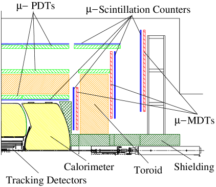
Figure 15: One quadrant of the DØ detector.

In the following paragraphs we discuss the subsystems of DØ in more details.

Tracking System

The inner tracking system comprises two major subsystems: a high precision silicon microstrip tracker (SMT) [157] and a scintillating fibre tracker [158]. The inner tracker is encased in a superconducting solenoid, which provides a magnetic field of 2 Tesla. The SMT consists of six barrel modules and 16 disk modules. Each barrel module has four radial layers of strip detector ladders which are arranged parallel to the beam axis. The layers are evenly spaced between radii of 2.5 and $10\,\mathrm{cm}$. Single- and double-sided detectors provide measurements in the $r$-$\phi$ and the $r$-$z$ views. Layers 2 and 4 feature double-sided detectors which have axial strips on each side with a small stereo angle of $2^{\circ}$ between the views. There is one disk module with 12 wedge shaped double-sided detectors at one end of each barrel. These disks are called F-disks. The silicon wafers on a disk module are oriented perpendicular to the beam axis and allow tracking at high pseudo-rapidities. At each end of the barrel assembly there are additional three F-disk modules. Thus, there is 12 F-disk modules in total. Further along the beam pipe, on each side of the detector, there are two larger disks of single-sided strip detectors (H-disks).

The Central Fibre Tracker (CFT) consists of scintillating fibres mounted on eight concentric cylinders which extend radially from $19.5\,\mathrm{cm}$ to $51.5\,\mathrm{cm}$. The detector is divided into 80 sectors in azimuth. Each sector contains 896 fibres, resulting in a total of 71680 channels. The CFT provides full angular coverage of the central region up to $|\eta|<1.7$. Charged particles passing through a fibre produce scintillation light that will travel along the fibre in both directions. At one end, an aluminium mirror reflects the light back into the fibre. At the other end, the fibre is joined to a wavelength shifting waveguide that transmits the light to silicon avalanche photodiodes, which convert the light into an electrical signal. The momentum resolution of the DØ tracking system can be parametrized by $\Delta p_{T}/p_{T}=\sqrt{0.015^{2}+(0.0014\,p_{T})^{2}}$, where $p_{T}$ is measured in GeV.

Calorimetry

DØ has a sampling calorimeter based on depleted uranium, lead and copper as absorber materials and liquid argon as sampling medium. The calorimeter consists of three cryostats: the Centre Calorimeter (CC), which covers the pseudorapidity region of $|\eta|<1.2$ and two endcap calorimeters (EC) which extend up to $|\eta|\approx 4$. The electromagnetic section of the calorimeter has a thickness of approximately 20 radiation lengths $X_{0}$. Calorimeter cells in the central region have a size of $\Delta\eta\times\Delta\phi=0.1\times 0.1$, except for the third layer of the electromagnetic section, where the grid size is $\Delta\eta\times\Delta\phi=0.05\times 0.05$ to provide better spacial resolution in the maximum of electromagnetic showers. At $\eta=0$, the CC has a total of 7.2 nuclear interaction lengths ($\lambda$), at the smallest angle of the EC the total is $10.3\,\lambda$. The energy resolution of the calorimeter is $\Delta E/E=15\%/\sqrt{E}\oplus 0.4\%$ for electrons and photons. For charged pions and jets the energy resolution is $50\%/\sqrt{E}$ and $80\%/\sqrt{E}$, respectively ($E$ is measured in GeV).

To improve electron identification DØ features a preshower detector which consists of two subsystems: the central system covering the region with $|\eta|<1.3$ (CPS) and the forward systems covering $1.5<|\eta|<2.5$ (FPS) [159]. Both subdetectors are based on a combination of lead radiator and scintillator layers. Electrons and photons shower in the radiator, while muons or charged pions only deposit energy due to ionization. In the central region the lead is mounted on the outer surface of the solenoid amounting to a total of $2\,X_{0}$. The scintillator is placed between the lead layer and the calorimeter. In the forward region, which is not fully covered by the tracking system, the radiator is sandwiched between two scintillator layers. Photons do not deposit energy in the first scintillator layer and can thereby be distinguished from electrons.

Muon System

The muon detector of DØ consists of three major components: (1) a toroid magnet which provides a magnetic field of $|\vec{B}|=1.8\;\mathrm{T}$, (2) the Wide Angle Muon Spectrometer (WAMUS) [160] covering the central region of $|\eta|<1.0$, and (3) the Forward Angle Muon Spectrometer (FAMUS) covering the area of $1.0<|\eta|<2.0$ [161]. Both spectrometers are based on layers of proportional drift tubes and scintillation counters. Being immersed in a magnetic field allows the muon system to provide a momentum measurement for muons independent of the inner tracker. This feature of DØ is a major difference to CDF where the muon momentum is determined by matching a muon stub to a track in the central tracker. The total amount of material in the calorimeter and the iron toroids varies between 13 and 19 nuclear interaction lengths, making the background from hadronic punch-through negligible.

Trigger and Data Acquisition

DØ has a three-tier system of triggers to select events for recording. The Level 1 trigger is a hardware based system with an output rate of 10 kHz [162]. Data coming from the preshower detector and the fibre tracker (CFT) are combined to form the Central Track Trigger (CTT) [163]. In addition, there are conventional calorimeter and muon triggers. Level 2 of the trigger system delivers an output rate to 1 kHz [164]. At the second trigger level information of all detector components can be combined at improved resolutions. Level 3, running high level software algorithms on a PC farm, further reduces the rate to 50 Hz.

Luminosity Measurement

At DØ the luminosity is measured by two hodoscopes located on the inside face of the calorimeters [165]. Each of these hodoscopes is made of 24 wedge shaped scintillators with fine mesh photo-multiplier tubes mounted on the face of each wedge. The hodoscopes cover the pseudorapidity region of $2.7<|\eta|<4.4$. The luminosity counters are designed to distinguish between single and multiple interaction events. The measurement of the rate of single inelastic interaction events is used to deduce the Poisson mean $\mu$ of the number of interactions per bunch-crossing. The instantaneous luminosity is then calculated by using $\mathcal{L}=\bar{f}\cdot\mu/\sigma_{inel}$ as discussed in Sec. 4.2. The luminosity measurement has an uncertainty of 7%.

4.4 Top quark signatures in $t\bar{t}$ events

In this section we discuss the experimental signature of top quark events. We constrain the discussion to the decay mode which dominates in the SM: $t\rightarrow W+b$ with a branching ratio close to 100%. We further concentrate on the signatures of $t\bar{t}$ events, since pair production is the main source of top quarks at the Tevatron and at the LHC. The signature of single top quark events and top quark decays via flavour changing neutral currents are presented in chapters 8.6 and 9.

Once both top quarks have decayed, a $t\bar{t}$ event contains two $W$ bosons and two $b$ quarks: $W^{+}W^{-}b\bar{b}$. Experimentally, $t\bar{t}$ events are classified according to the decay modes of the $W$ bosons. There are three leptonic modes ($e\nu_{e}$, $\mu\nu_{\mu}$, $\tau\nu_{\tau}$) and six decay modes into quarks of different flavour ($u\bar{d}$, $u\bar{s}$, $u\bar{b}$, $c\bar{d}$, $c\bar{s}$, $c\bar{b}$). We distinguish four $t\bar{t}$ event categories:

1. Both $W$ bosons decay into light leptons (either $e\nu_{e}$ or $\mu\nu_{\mu}$) which can be directly seen in the detector. This category is called dilepton channel.

2. One $W$ boson decays into $e\nu_{e}$ or $\mu\nu_{\mu}$. The second $W$ decays into quarks. This channel is called lepton-plus-jets.

3. Both $W$ bosons decay into quarks. We refer to this mode as the all hadronic channel.

4. At least one $W$ boson decays into a tau lepton ($\tau\nu_{\tau}$) which itself can decay either leptonically (into $e\nu_{e}$ or $\mu\nu_{\mu}$) or hadronically into quarks.

In good approximation we can neglect all lepton masses with respect to the $W$ mass and write:

$$\Gamma^{0}_{W}\equiv\Gamma(W\rightarrow e\nu_{e})=\Gamma(W\rightarrow\mu\nu_{\mu})=\Gamma(W\rightarrow\tau\nu_{\tau})$$

At lowest order in perturbation theory the decay rate into a quark-antiquark pair, $q_{1}\bar{q}_{2}$, is given by the rate into leptons $\Gamma^{0}_{W}$ multiplied by the square of the CKM matrix element $|V_{q_{1}q_{2}}|^{2}$ and enhanced by a colour factor of 3, which takes into account that quarks come in three different colours:

$$\Gamma(W\rightarrow q_{1}\bar{q}_{2})=3\,|V_{q_{1}q_{2}}|^{2}\;\Gamma^{0}_{W}\ .$$

The hadronic decay width $\Gamma_{\mathrm{had}}$ of the $W$ is summed over all six quark-antiquark modes

$$\Gamma_{\mathrm{had}}=3\,\Gamma^{0}_{W}\cdot\sum_{q_{1}q_{2}}|V_{q_{1}q_{2}}|^{2}\ \ \ \mathrm{with}\ \ \ q_{1}q_{2}\in\{ud,us,ub,cd,cs,cb\}.$$

The unitarity of the CKM matrix demands that the sum over the CKM elements squared is equal to 2 and one obtains $\Gamma_{\mathrm{had}}=6\,\Gamma^{0}_{W}$. As a result, each leptonic channel has a branching ratio of 1/9, while the hadronic decay channel into two quarks has a branching ratio of 6/9. For the $t\bar{t}$ decay categories we get thus the probabilities as listed in Tab. 7.

Table 7: Categories of $t\bar{t}$ events and their branching fractions.

$W$ decays	$e/\mu\nu$	$\tau\nu$	$q\bar{q}$
$e/\mu\nu$	4/81	4/81	24/81
$\tau\nu$	–	1/81	12/81
$q\bar{q}$	–	–	36/81

(i) Dilepton mode: 4/81, (ii) lepton-plus-jets: 24/81, (iii) all-hadronic channel: 36/81, (iv) tau modes: 17/81. These four different types of $t\bar{t}$ events can be isolated by their distinct event topologies.

Dilepton Channel

This final state includes (1) two high $p_{T}$ leptons, electron or muon, (2) a large imbalance in the total transverse momentum (missing transverse energy, $E_{\mathrm{T}}\!\!\!\!\!\!\!/\ \;$) due to two neutrinos, and (3) two $b$ quark jets. The dilepton event category has low backgrounds, especially in the $e\mu$ channel, since $Z^{0}$ mediated events do not contribute. However, the drawback of the dilepton channel is its low branching ratio of about 5%. There is a small contribution from tau events to the dilepton channel, if the tau decays into $e$ or $\mu$. This cross feed has to be taken into account when calculating acceptances for dilepton analyses. Since dilepton events contain two neutrinos which contribute to the $E_{\mathrm{T}}\!\!\!\!\!\!\!/\ \;$, the top quarks cannot be fully reconstructed. This is a drawback if one wants to measure the top quark mass. However, this disadvantage is partially compensated by the precisely measured lepton momenta, in contrast to the only fair measurement of jet energies in the lepton-plus-jets channel.

Lepton-Plus-Jets Channel

The lepton-plus-jets channel is characterised by (1) exactly one high-$p_{T}$ electron or muon, which is also called the primary lepton, (2) missing transverse energy, (3) two $b$ quark jets from the top decays, and (4) two additional jets from one $W$ decay. An event display of a lepton-plus-jets candidate event measured at CDF II is shown in figure 16.

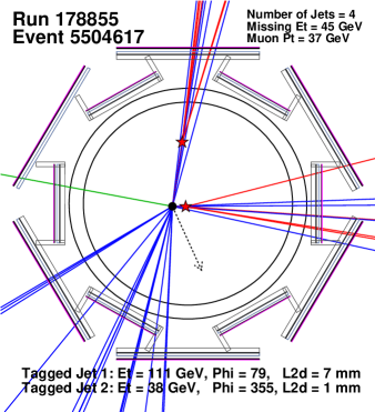
Figure 16: Event display of a CDF II muon-plus-jets event. The isolated line on the left hand side shows the muon trajectory. The arrow on the lower right indicated the direction of the $\bi{E}_{\mathrm{T}}\!\!\!\!\!\!\!/\;\;$. The event features four hadronic jets.

The big advantage of the lepton-plus-jets channel is its high branching fraction of about 30%. The backgrounds are considerably higher than in the dilepton channel, but still manageable. Several strategies of background suppression have been developed and are discussed in section 6.2. Again, as in the dilepton channel, there is some cross feed from tau modes which has to be taken into account for acceptances. In lepton-plus-jets events the momentum of the leptonically decaying $W$ boson can be reconstructed up to a twofold ambiguity. The transverse momentum of the neutrino is assumed to be given by $E_{\mathrm{T}}\!\!\!\!\!\!\!/\ \;$. Two solutions for the $z$ component of the neutrino are obtained from the requirement that the reconstructed invariant mass of the lepton and the neutrino be equal to the well known $W$ mass: $M_{\ell\nu}=M_{W}$. To fully reconstruct the momenta of the top and antitop quark in the event, one has to assign the measured hadronic jets to the quarks. Without identification of $b$ quark jets there are 24 possible combinations, including the ambiguity of the neutrino reconstruction. If one jet is identified as likely to originate from a $b$ quark 12 combinations remain. If there are two identified $b$ jets the ambiguity is down to 4 options. This illustrates the importance of $b$ quark jet identification for top quark physics.

All Hadronic Channel

The all hadronic channel has the largest branching ratio out of all $t\bar{t}$ event categories, about 44%. However, backgrounds are quite considerable. While there is the advantage that all final state partons are measured, one has to deal with numerous combinations when reconstructing the top quark momenta. Even if two jets are identified as $b$ quark jets, 12 possible combinations remain. Another drawback is that jet energies as measured in the calorimeter have large uncertainties. The combination of these disadvantages leads to the conclusion that the all hadronic channel, even though a clear $t\bar{t}$ signal has been established here, proves not very useful to further investigate top quark properties.

Tau Modes

Top quark events containing the decay $W\rightarrow\tau\nu_{\tau}$ are difficult to identify and have not been seen to date. The search for this decay mode is briefly described in section 8.3.

4.5 Particle detection and identification

In the previous section we have explained $t\bar{t}$ signatures in terms of primary partons. In this section we will discuss how these partons are detected and how their properties are measured.

4.5.1 Electrons and muons

Charged leptons emerging from a decay of a $W$ boson have high transverse momenta that can be measured by the tracking system with good resolution. Electrons interact within the first few segments of the calorimeter and form electromagnetic showers of photons and electron-positron pairs. To select electrons from $W$ decays one typically requires a transverse energy, $E_{T}=E\cdot\sin\theta$, of at least 20 GeV. The energy resolution (at CDF for example) is $\sigma(E_{T})/E_{T}=13.5\%/\sqrt{E_{T}}\oplus 2\%$, where $E_{T}$ is measured in GeV. The shower should be mainly contained in the electromagnetic part of the calorimeter. A typical requirement is that 90% of the total measured energy is observed in the electromagnetic calorimeter. Moreover, there must be a track that, if extrapolated to the calorimeter, matches the location of the electromagnetic shower and has a momentum consistent with the shower energy ($E/p\sim 1$). Additional requirements include the transverse and longitudinal shapes of the shower, which are known from test beam data. Energetic photons that interact with detector material prior to their entry into the tracking system and produce an electron-positron pair can mimic high-$p_{T}$ primary electrons and pose a serious background. One can identify and veto these conversion pairs if both, the electron and the positron track, are reconstructed and fulfil a matching criterion with respect to a common vertex. The major background to high-$p_{T}$ electrons arises from hadronic showers developing early in the calorimeter and depositing most of their energy in the electromagnetic section. Such a case can, e.g., be caused by photons from $\pi^{0}$ decays. The hadronic jet background can be considerably suppressed by exploiting the fact that leptons coming from a heavy boson decay are isolated from other jet activity in the event. Thus, it is asked that the electron shower is isolated from other energy deposits in the calorimeter. A typical requirement is that the energy measured in an annulus of radius $\Delta R=0.4$ around the electron shower is less than 10% of the shower energy.

Muons can be reliably identified as tracks that penetrate the calorimeter as well as additional shielding material and reach the outmost layers of the collider experiment, the muon system. The track is typically required to have a transverse momentum of at least 20 GeV/c and match, when extrapolated through the calorimeter, a short track segment measured in the muon system. Uncertainties due to multiple scattering in the calorimeter and the shielding material have to be considered accordingly in the matching criteria. The transverse momentum of high-$p_{T}$ muons is measured with a typical resolution of $\sigma(p_{T})/p_{T}=0.1\%\,p_{T}$, where $p_{T}$ is given in GeV/$c$. The energy measured in the calorimeter segment containing the muon is required to be consistent with the deposition expected from a minimum ionizing particle. Muons are required to be isolated from additional calorimeter activity as described above for electrons. Real muons from cosmic rays have to be distinguished from muons originating from hadronic collisions and removed from the data sample. One requires that the muon track extrapolates to the primary collision point of the event. Timing information of the tracker and the calorimeter are used to ensure that the passage of the muon through the primary interaction region falls into a narrow time window around the beam crossing, that is known from the accelerator clock signal. Other backgrounds to the muon signal arise from pion or kaon decays in flight, or from hadrons that traverse the calorimeter and the absorber material without producing a hadronic shower (punch-through).

High-$p_{T}$ electrons and muons can be speedily reconstructed with good precision and are used in the trigger systems of collider experiments to select events containing heavy gauge bosons and other high-$p_{T}$ events in real time. The primary data samples for $t\bar{t}$ dilepton and lepton-plus-jets events are defined in this way.

4.5.2 Neutrinos

Neutrinos interact only weakly with matter and therefore cannot be directly observed in a collider detector. Instead their presence is inferred from an imbalance in the total transverse energy of the event. As described in section 3.1.1 the hard scattering in hadronic collisions happens between two partons whose momentum fraction is a-priori unknown. The remnants of the colliding hadrons, the spectator partons that do not participate in the hard interaction, have little transverse momentum and escape undetected down the beam pipe. In contrast to $e^{+}e^{-}$ collisions one can therefore not simply invoke energy and momentum conservation before and after the collisions. However, the total transverse momentum is conserved and is known to be zero before the collision. Any imbalance in the vector sum of transverse momenta can therefore be attributed to the presence of neutrinos that carry away momentum undetected. In practice, one cannot determine the momenta of all particles produced in the collision, but rather measures the imbalance of energy in the calorimeter. To each calorimeter cell $i$ one assigns a transverse energy vector $\bi{E}_{\mathrm{T}}^{i}=(E_{i}\sin\theta_{i}\cos\phi_{i},\;E_{i}\sin\theta_{i}\sin\phi_{i})$ and calculates the sum over all cells: $\bi{E}_{\mathrm{T}}\!\!\!\!\!\!\!/\;\;=-\sum_{i}\bi{E}_{\mathrm{T}}^{i}$. Here $\theta_{i}$ and $\phi_{i}$ are the angular coordinates of calorimeter cell $i$. Since muons loose only a minimal amount of their energy in the calorimeter, $\bi{E}_{\mathrm{T}}\!\!\!\!\!\!\!/\;\;$ has to be corrected for identified muons. The limiting factor on the resolution of $E_{\mathrm{T}}\!\!\!\!\!\!\!/\ \;=|\bi{E}_{\mathrm{T}}\!\!\!\!\!\!\!/\;\;|$ is the uncertainty in the measurement of hadronic jet energies in the calorimeter. Therefore, one usually parametrizes the $E_{\mathrm{T}}\!\!\!\!\!\!\!/\ \;$ resolution in terms of the scalar sum of all transverse energies in the event, $\sum E_{\mathrm{T}}$, measured in GeV. For $t\bar{t}$ dilepton candidate events CDF has measured a resolution of $\sigma(E_{\mathrm{T}}\!\!\!\!\!\!\!/\ \;)=0.7\cdot\sqrt{\sum E_{\mathrm{T}}}$ [166]. DØ determined its $E_{\mathrm{T}}\!\!\!\!\!\!\!/\ \;$ resolution for minimum bias data and quotes $\sigma(E_{\mathrm{T}}\!\!\!\!\!\!\!/\ \;)=1.08\;\mathrm{GeV}+0.019\;\sum E_{\mathrm{T}}$ [167].

4.5.3 Jets of quarks and gluons

The strength of the strong force increases with distance and prevents elementary particles carrying colour charge, i.e. quarks and gluons, from existing as free objects. Quarks and gluons are confined to exist in hadrons, which are colour singlets. In collider experiments quarks and gluons participate in the hard interaction and subsequently form collimated jets of hadrons which can be observed in a detector. Jets tend to preserve the direction of motion of the original parton. In the calorimeter they are detected as an extended cluster of energy. To compare measurements with theoretical predictions a precise mathematical prescription is necessary how to form jets out of energy clusters measured in the calorimeter. Different jet algorithms are available, but at hadron colliders calorimeter cells are conventionally combined within a cone of fixed radius $\Delta R$ in $\eta$-$\phi$ space, because jets are approximately circular in the $\eta$-$\phi$ plane. Moreover, in this parametrization the size of a jet of a particular $E_{\mathrm{T}}$ is independent of the jet rapidity. The cone size $\Delta R$ is chosen differently depending on the physics analysis. On one hand the cone must be big enough, such that most of the energy associated to the original quark is contained in the jet cone. On the other hand the cone size should be small enough, such that energy depositions corresponding to different primary partons are resolved individually rather than merged to one jet. This is especially a concern for $t\bar{t}$ events which have many jets in their final state. At the Tevatron the optimal choice was found to be $\Delta R=0.4$ for CDF and $\Delta R=0.5$ for DØ. The difference between the two experiments reflects a small dependence on the calorimeter design and geometry.

Both Tevatron experiments feature an energy resolution for jets of $\sigma(E_{\mathrm{T}})/E_{\mathrm{T}}\approx 100\%/\sqrt{E_{\mathrm{T}}}$, where $E_{\mathrm{T}}$ is measured in GeV. Several systematic effects compromise the jet energy measurement: (1) intrinsic large fluctuations in the response of calorimeters to hadronic showers, (2) nonlinear effects in calorimeter response, (3) calorimeter non-uniformities and energy loss in uninstrumented regions, such as cracks between modules, (4) increase in energy due to the overlap of multiple hard interactions in one bunch crossing, (5) energy of the underlying event feeding into the jet cone (The underlying event consists of particles coming from the fragmentation of partons that do not participate in the hard scattering of the primary $p\bar{p}$ or $pp$ interaction.), and (6) energy loss due to the use of a finite cone size in jet reconstruction. To understand these effects experimentally turns out to be one of the major challenges in collider physics. Appropriate correction methods have to be derived and the detector simulation has to be tuned to describe the measurements.

Calorimeter calibration commonly starts with the electromagnetic section for which an absolute energy scale can be derived by comparing electron energies measured in the calorimeter to their momenta measured in the tracking system or by reconstructing resonances with well known masses such as the $Z$ boson, the $\pi^{0}$ or the $J/\psi$. In a second step the hadronic part of the calorimeter can be calibrated against the electromagnetic part by studying photon-plus-one-jet events, where the transverse energies should balance. Dijet events are further used to calibrate one hadronic region of the detector relative to another better understood region. Contributions from the underlying event are investigated by Monte Carlo simulations and comparison to data taken under special trigger conditions and luminosities.

Finally, it has to be noted that one cannot achieve a one-to-one correspondence of primary quarks and gluons and the observed jets in all kinematic regions and for all event topologies of a certain physics process, and one cannot expect to do so. To define jets a minimum of transverse energy is required. One may start counting soft jets with $8\,\mathrm{GeV}$. However, this can complicate discrimination between signal and background. In most $t\bar{t}$ analyses jets are typically defined with $E_{\mathrm{T}}>15\,\mathrm{GeV}$. This threshold causes, e.g., some $t\bar{t}$ lepton-plus-jets events to have only three instead of four jets. Another source of inefficiency in jet reconstruction is the merging of jets which are close together in $\eta$-$\phi$ space and cannot be resolved separately. Conversely, if a parton radiates a gluon with large relative transverse momentum, that gluon can be reconstructed as an additional jet.

4.5.4 Tagging of $b$ quark jets

As pointed out in section 4.4, $t\bar{t}$ events feature two energetic $b$ quark jets, while the heavy flavour content in background events is relatively low. Therefore, the identification, also called the tagging, of $b$ quark jets is an important tool to suppress background, enrich top quark data samples, and to facilitate the full reconstruction of top quark momenta by reducing the number of possible combinations of final state objects. In this section we briefly present three $b$ tagging methods employed at hadron colliders. The first two methods are based on the relatively long lifetime of $b$ hadrons, which is about $1.5\,\mathrm{ps}$. Since $b$ hadrons emerging from top quark decays have relatively high momenta, their long lifetime allows them to travel several mm before decaying. Tracks from a $b$ hadron decay therefore typically originate from a secondary vertex that is displaced from the primary interaction point. The first $b$ tagging method reconstructs the secondary vertex of $b$ hadrons within a jet and bases the $b$ tag on the significance of the displacement. The second method searches for tracks with large impact parameter with respect to the primary vertex, but does not require the reconstruction of the secondary vertex itself. The third method identifies leptons at intermediate momenta (typically: $2\,\mathrm{GeV}/c<p_{\mathrm{T}}<20\,\mathrm{GeV}/c$) from semileptonic $b$ decays within jets. Since momenta of these leptons are much smaller than those of leptons coming from $W$ or $Z$ boson decays, this method is also called soft lepton tag.

Secondary vertex tag

The secondary vertex method identifies $b$ jets by establishing a displaced secondary vertex in the jet from the decay of a long lived $b$ hadron. The following explanation goes along the lines of the algorithm employed by CDF, but the DØ version is quite similar. In a first step the space point of the hard primary interaction is precisely reconstructed. One starts by clustering the $z$ coordinates of all tracks at the point of their closest approach to the origin (perigee). After applying several quality requirements this procedure yields an estimate of the $z$ position of the primary vertex, $z_{\mathrm{pv}}$. The trajectory of the proton and antiproton beams through the collision region, also called the beamline, is known with high precision, $\mathcal{O}(1\,\mu\mathrm{m})$, from subsidiary measurements made on a run-by-run basis. Combining $z_{\mathrm{pv}}$ with the beamline yields a first estimate of the primary vertex position $\bi{x}_{\mathrm{pv}}$. The precision of $\bi{x}_{\mathrm{pv}}$ is subsequently improved by including tracks with low impact parameter significance into a full vertex fit. As a result, the uncertainty on the transverse position of the primary vertex ranges from about 10 – $30\,\mu\mathrm{m}$, depending on the number of tracks and the event topology.

The subsequent steps of secondary vertex tagging are performed on a per-jet basis. Only tracks within the jet cone are considered. To ensure good track quality cuts involving the transverse momentum, the significance of their impact parameter $d$ relative to $\bi{x}_{\mathrm{pv}}$, $d/\sigma_{d}$, the number of silicon hits attached to a track, the quality of those hits, and the quality of the final track fit are applied. Tracks consistent with coming from the decays $K_{s}^{0}\rightarrow\pi^{+}\pi^{-}$ or $\Lambda\rightarrow\pi^{-}p$, or photon conversions are not accepted as good candidate tracks. For a jet to be taggable at least two good tracks have to fall within the jet cone. One iterates over the set of good tracks and tries to fit them to a common vertex with a certain minimum fit quality ($\chi^{2}$ per degree of freedom).

Once a secondary vertex is found in a jet, the two-dimensional decay length $L_{\mathrm{2D}}$ of the secondary vertex is calculated. $L_{\mathrm{2D}}$ is the projection of the vector pointing from the primary to the secondary vertex onto the jet axis in the $xy$ plane. The sign of $L_{\mathrm{2D}}$ is determined by the angle between the jet axis and the secondary vertex vector in the $xy$ plane. If the angle is $<90^{\circ}$ the sign is positive, if the angle is $>90^{\circ}$, the sign is negative. Large positive values of $L_{\mathrm{2D}}$ are predominantly attached to vertices of real $b$ hadron decays, while displaced vertices with negative $L_{\mathrm{2D}}$ are mainly due to track mismeasurements or random combinations of tracks. To reduce the background from false secondary vertices, called mistags, a good secondary vertex is required to have a minimum decay length significance of typically $L_{\mathrm{2D}}/\sigma_{\mathrm{2D}}>3$, where $\sigma_{\mathrm{2D}}$ is the estimated uncertainty on $L_{\mathrm{2D}}$. The uncertainty $\sigma_{\mathrm{2D}}$ is estimated for each vertex individually, a typical value is about $200\,\mathrm{\mu m}$. Figure 17a shows the distribution of $L_{\mathrm{2D}}$ as obtained in a CDF measurement of the $t\bar{t}$ cross section [168]. The distribution has the form of a falling exponential, as expected from a lifetime distribution. The content of the first bin is exceptionally lower due to the cut on the decay length significance, $L_{\mathrm{2D}}/\sigma_{\mathrm{2D}}>3$. More detailed descriptions of secondary vertex $b$ tagging can be found in references [166, 103] (CDF Run I), reference [168] (CDF Run II) and references [169, 170] (DØ Run II). In the latest CDF analysis (Run II) the efficiency of tagging at least one $b$ quark jet in a $t\bar{t}$ event is (53$\pm$3)% [168]. This number includes the geometric acceptance of tracks from $b$ decays (taggability). The estimated uncertainty is purely systematic.

   (a)                                                                       (b)

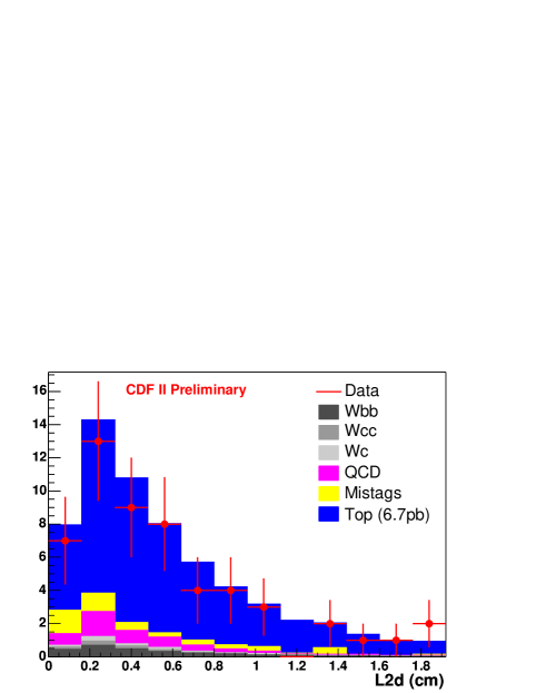
Figure 17: (a) Two-dimensional decay length $L_{\mathrm{2D}}$ of secondary vertices as obtained in a CDF measurement of the $t\bar{t}$ cross section [168]. (b) Distribution of the signed impact parameter significance of tracks in a jet data sample, where there is at least one jet with $E_{\mathrm{T}}>50\,\mathrm{GeV}$ per event. The data are fit with a resolution function consisting of two Gaussians plus an exponential function, separately for the positive and negative sides [103].

Impact parameter tag

The impact parameter $b$ tag algorithm compares track impact parameters to measured resolution functions in order to calculate for each jet the probability that there are no long lived particles in the jet cone. For light quark or gluon jets this probability is uniformly distributed between 0 and 1, while it is very small for jets containing tracks from displaced vertices of heavy flavour decays. The impact parameter significance $S_{0}$ is defined as the ratio of the impact parameter $d$ and its uncertainty $\sigma_{d}$. The sign of $d$ is defined to be positive if the point of closest approach to the primary vertex lies in the same hemisphere as the jet direction, and negative otherwise. Figure 17b shows the $S_{0}$ distribution of tracks in a jet data sample. The distribution is fit with a resolution function. The negative side of the resolution function is used to compute the probability $P(S_{0})$ that the $S_{0}$ of a particular track is due to detector resolution. The probability that a jet is consistent with a zero lifetime hypothesis is essentially given by the product of the individual probabilities $P(S_{0})$ of tracks contained in the jet cone including an appropriate normalization. Tracks used in the calculation of the jet probability are required to satisfy certain quality criteria involving a cut on the impact parameter, the transverse momentum and the number of hits in the silicon detector. The impact parameter tagging method has the advantage of providing a continuous variable, the jet probability, to distinguish between light and heavy flavour jets, which easily allows it to choose a certain value of $b$ tagging efficiency by adjusting the cut value on the jet probability. In addition, the probability value can be used in subsequent steps of an analysis, e.g. when applying multivariate techniques.

Soft Lepton Tag

The Soft Lepton Tag (SLT) is based on the identification of leptons originating from semileptonic $b$ decays $b\rightarrow\ell+X$, where the lepton is either an electron or a muon. Contributions come from the decay mode $b\rightarrow c\ell\nu$ or the sequential decay $b\rightarrow c\rightarrow s\ell\nu$. The semileptonic branching ratio of $b$ and $c$ hadrons is measured to be about 10% per lepton species ($e$ or $\mu$) [10]. This means that about 80% of $t\bar{t}$ events have at least one lepton from a semileptonic decay. In contrast to leptons from $W$ decays the leptons from $b$ decays are not isolated, but are rather contained in the cone of the $b$ quark jet. Their $p_{\mathrm{T}}$ spectrum is much softer, typically well below $20\,\mathrm{GeV}/c$. Therefore, the detection and identification of these leptons is much more difficult. In Run II, DØ  and CDF have used only muons for the soft lepton tag so far. DØ selects muons in the transverse momentum range of $4\,\mathrm{GeV}/c<p_{\mathrm{T}}<15\,\mathrm{GeV}/c$ and achieves a $b$ jet tagging efficiency of 11% [170].

4.6 Generation and simulation of Monte Carlo events

Collider experiments are intricate devices and predicting the experimental response to a certain physics process is non-trivial. To extract sensible information from data one needs first an accurate modelling of the event kinematics and topology on parton and hadron level, and second a detailed simulation of the detector response to particles interacting with the detector material.

There are two commonly used general purpose Monte Carlo event generators, Pythia [171] and Herwig [172], which provide an exclusive description of individual events at hadron level. They are based on leading order matrix elements for the hard parton scattering convoluted with parametrizations of parton distribution functions and include approximate treatments of higher order perturbative effects, initial and final state gluon emission, parton shower, hadronization, secondary decays and the underlying event. The strength of Pythia and Herwig is the modelling of the parton shower, where outgoing partons are converted into a cascade of gluons and $q\bar{q}$ pairs with energy and angular distributions determined by the DGLAP equations, which describe the $Q^{2}$ evolution of quark and gluon densities [173, 174, 175]. The parton shower is terminated when the virtual invariant mass of the parton ($Q^{2}$) falls below a threshold value chosen such that a perturbative treatment is valid above the threshold. The evolution of the shower beyond this stage is determined by non-perturbative physics. The partons are turned into colourless hadrons according to phenomenological hadronization (or fragmentation) models. Particles originating from interactions of the beam remnants are also included in the model and are called the underlying event. A set of parameters is tuned to reproduce hadron multiplicities and transverse momentum spectra of the underlying event as measured in soft $p\bar{p}$ collisions, so called minimum bias events. To obtain a proper modelling of $b$ and $c$ hadron decays, heavy flavor jets are interfaced to the decay algorithm QQ which comprises tables of the most up to date branching fractions.

While Pythia and Herwig provide a good description of $t\bar{t}$ events [176], they are insufficient to model multijet and $W$ + multijet background events. Particularly critical is the generation of $W$ + heavy flavour jets. In Run I of the Tevatron $W$ + jets events were generated with the Vecbos Monte Carlo program [177], in Run II the Alpgen program is used [178], which generates high multiplicity partonic final states based on exact leading order matrix elements. The parton level events are passed to Herwig for showering and hadronization and to QQ for the decay of heavy flavour hadrons. To reproduce the entire $W$ + multijets spectrum several Alpgen samples have to be accurately merged together.

Monte Carlo event generators output a list of stable particles which can be fed to a full detector simulation that reproduces the interaction of those particles with the detector material. The simulation code is based on the Geant package [179] which allows to implement a detailed geometry description of the detector, track particles through the given detector volumes and compute their energy loss as well as multiple scattering. In the so called digitization step the energy depositions obtained from Geant are converted into raw detector data which are in the same format as physics data recorded from real collisions. Most detectors are described by parametric models that convert energy deposits into detector signals. The parameters of the models are tuned to correctly reproduce the detector response. The silicon detector response, for example, can be modelled by a simple geometrical model based on the path length of the ionizing particle and a Landau distribution measured from physics data. The raw data obtained from Monte Carlo events are then subjected to the same reconstruction code as data from collisions. These reconstructed Monte Carlo data can then be analysed in the same way as if they would contain physics events. Monte Carlo samples generated in this way are used to compute acceptances for certain physics processes and to compare kinematic distributions between data and predictions.

5 The quest for the top quark

Immediately after the discovery of the $b$ quark in 1977 the existence of a weak isospin doublet partner, the top quark, was hypothesised. The mass of the sixth quark was unknown and a wealth of predictions appeared based on many different speculative ideas, see for example references [180, 181, 182]. Typical expectations were in the mass range of about $20\,\mathrm{GeV}/c^{2}$, which became accessible two years later with measurements at the PETRA $e^{+}e^{-}$ collider.

5.1 Early searches

In $e^{+}e^{-}$ annihilations $t\bar{t}$ pairs can be produced by the exchange of a virtual photon or $Z$ boson. The mass hierarchy of Standard Model quarks is beautifully reflected in a measurement of the ratio of the production rate of hadrons to that for muon pairs, $R=\sigma(e^{+}e^{-}\rightarrow\mathrm{hadrons})/\sigma(e^{+}e^{-}\rightarrow\mu^{+}\mu^{-})$, as a function of the centre-of-mass energy $\sqrt{s}$. The ratio $R$ is given by $R(s)=3\;\sum Q_{i}^{2}$, where the sum is over all quark flavours with production thresholds greater than $\sqrt{s}$. This corresponds to a step function, which is only altered near production thresholds where strong resonance effects occur. If one compares $R$ above the $t\bar{t}$ production threshold to its value below (but above the threshold for $b\bar{b}$ production) one expects to see an increase by $\Delta R=4/3$.

Between 1979 and 1984 the five experiments at the PETRA collider, CELLO, JADE, MARK J, PLUTO, and TASSO, measured $R$ at several centre-of-mass energies ranging from 12 to 46.8 GeV in steps of about 20 to 30 MeV [183, 184, 185, 186, 187]. No indication of top quark production was found. The final lower limit of the top quark mass derived from PETRA measurements was $23\,\mathrm{GeV}/c^{2}$.

At the KEK laboratory in Japan a dedicated accelerator, TRISTAN, was built to search for the top quark in $e^{+}e^{-}$ annihilations, with slightly increased centre-of-mass energy than PETRA. The maximum energy reached was 61.4 GeV. Between 1987 and 1990 several consecutive searches for top quark production were presented by the two experiments operating at TRISTAN (AMY and VENUS). Again, no evidence for the top quark was found and the final lower limit on the top quark mass was 30.2 GeV/$c^{2}$ [188, 189].

In 1989 the Large Electron Position collider (LEP) at CERN and the Stanford Linear Collider (SLC) started $e^{+}e^{-}$ collisions at the $Z^{0}$ pole, $\sqrt{s}\approx 90\;\mathrm{GeV}$. The experiments at these accelerators – ALEPH, DELPHI, OPAL and L3 at LEP, and SLD at SLC – searched for $Z^{0}\rightarrow t\bar{t}$ events of various topologies [190, 191, 192, 193]. The best lower limit on the top quark mass obtained from these direct searches was $45.8\,\mathrm{GeV}/c^{2}$.

In the mid 1980s experiments at hadron colliders joined experiments at $e^{+}e^{-}$ machines in the quest for the top quark. In contrast to $e^{+}e^{-}$ annihilations, searches in hadronic collisions have to deal with high backgrounds and thus model independent analyses are not feasible. Instead the experiments had to concentrate on SM signatures. Initially, one assumed the top quark mass to be below the mass of the $W$ boson. Top quark production via the electroweak interaction was expected to be the dominating process at the CERN $Sp\bar{p}S$ collider operating at $\sqrt{s}=546\;\mathrm{GeV}$, later at $\sqrt{s}=630\;\mathrm{GeV}$. The experiments UA1 and UA2 searched for events were an on-shell $W$ boson is produced which decays into a top and a bottom quark: $p\bar{p}\rightarrow W^{\pm}\rightarrow t\bar{b}/\bar{t}b$. The top quark was reconstructed in its semileptonic decay mode into a $b$ quark, a charged lepton (electron or muon) and a neutrino.

First results reported by UA1 in 1984 seemed to be consistent with the production of top quarks of mass $(40\pm 10)\,\mathrm{GeV}/c^{2}$ [194]. UA1 observed six events with one isolated lepton, 3 electron and 3 muon events, and 2 hadronic jets. The effective invariant mass distribution of the lepton, the two jets and the missing transverse energy shows a pronounced peak at the $W$ mass, while the mass of the lepton, the missing transverse energy and the jet with the lowest transverse energy clustered around 40 GeV/$\mathrm{c^{2}}$. The number of background events where the lepton was faked by a hadron or background events from heavy flavour production were believed to be negligible. Thus, these six events were interpreted as a first indication of a top quark originating from a $W$ boson decay. However, subsequent analyses by UA1 were based on a more complete evaluation of the backgrounds and did not support this result [195]. Since UA1 did not apply a minimum cut on the missing transverse energy in the event, backgrounds due the fake leptons, Drell-Yan production of lepton pairs, $\ell^{+}\ell^{-}$, as well as backgrounds from $b\bar{b}$ and $c\bar{c}$ production were found to be more significant than originally estimated.

The final UA1 top quark analysis was published in 1990 and used data corresponding to an integrated luminosity of 5.4 $\mathrm{pb^{-1}}$. The observed events were found to be consistent with the non-top backgrounds, and a lower limit on the top quark mass of $60\,\mathrm{GeV}/c^{2}$ was set [196]. A slightly better limit was achieved by the second experiment operating at the CERN $Sp\bar{p}S$, UA2, based on an integrated luminosity of 7.1 $\mathrm{pb^{-1}}$ [197]. UA2 used only events containing an isolated central electron with $p_{\mathrm{T}}^{e}>12\;\mathrm{GeV}/c$ and $E_{\mathrm{T}}\!\!\!\!\!\!\!/\ \;>15\;\mathrm{GeV}$. After all selection cuts 137 events were retained, in good agreement with the expectation of $154.4\pm 14.6$ background events. To further enhance the sensitivity of the analysis the transverse mass of the electron and the missing transverse energy

$$M_{\mathrm{T}}^{e\nu}=\sqrt{\;2\,p_{\mathrm{T}}^{e}\,E_{\mathrm{T}}\!\!\!\!\!\!\!/\ \;\cdot(1-\cos\Delta\phi_{e\nu})\;}$$

was formed, where $\Delta\phi_{e\nu}$ is the azimuthal angle between the electron and $\bi{E}_{\mathrm{T}}\!\!\!\!\!\!\!/\;\;$ vectors. The limit on the top quark mass were obtained by fitting the observed $M_{\mathrm{T}}^{e\nu}$ distribution to template distributions of background events alone or a combination of background and a top quark signal of certain mass. As a result, top quark masses below $69\,\mathrm{GeV}/c^{2}$ were excluded.

It is important to note that experiments at hadron colliders do not provide a direct limit on the top quark mass, but rather on the top quark production cross section. The mass limits are derived using the theoretically predicted production cross sections, that depend on the top quark mass, and the predicted branching ratios. Systematic uncertainties on these predictions have thus to be properly accounted for.

5.2 Searches and discovery at the Tevatron

In 1988 the CDF experiment at the Tevatron joined the race for discovery of the top quark. Due to the higher centre-of-mass energy at the Tevatron of $\sqrt{s}=1.8\;\mathrm{TeV}$ top quarks are predominantly produced as $t\bar{t}$ pairs. The first CDF top quark search uses a data sample with an integrated luminosity of 4.4 $\mathrm{pb^{-1}}$ accumulated in Run 0 which lasted from 1988 to 1989 [198, 199]. CDF pursued a similar strategy as UA2 and used the $M_{\mathrm{T}}^{e\nu}$ distribution to discriminate between $W$+jets background events, where the $W$ boson decays on shell, and top quark decays where the electron and the neutrino originate from the exchange of a virtual $W$ (this was still under the assumption that $M_{\mathrm{top}}<M_{W}+M_{b}$). The analysis is based on isolated central electron events with an electromagnetic transverse energy above 20 GeV and $E_{\mathrm{T}}\!\!\!\!\!\!\!/\ \;>20\;\mathrm{GeV}$. In addition, at least two hadronic jets with $E_{\mathrm{T}}>10$ GeV and $|\eta|<2.0$ are required. This analysis pushed the lower limit of the top quark mass to $M_{\mathrm{top}}>77\,\mathrm{GeV}/c^{2}$ using predictions of the cross section by Altarelli et al. [89, 85].

In addition to the search in the electron-plus-jets channel CDF performed an analysis in the electron-plus-muon ($e\mu$) dilepton channel [200]. By requiring two leptons from different families, backgrounds from Drell-Yan and $Z^{0}$ production as well as $W$+jets events are strongly suppressed. The remaining background is mainly due to $Z^{0}\rightarrow\tau^{+}\tau^{-}$ events. Subsequently, CDF extended the dilepton analysis to include the $ee$ and $\mu\mu$ channels. Backgrounds from Drell-Yan and $Z^{0}$ events are reduced by additional requirements: (1) The dilepton azimuthal opening angle $\Delta\phi_{\ell\ell}$ is required to be below $160^{\circ}$. (2) $ee$ or $\mu\mu$ events with a dilepton invariant mass in the window $75<M_{\ell\ell}<105\;\mathrm{GeV}/c^{2}$ or with $E_{\mathrm{T}}\!\!\!\!\!\!\!/\ \;<20\;\mathrm{GeV}$ are rejected. The lepton+jets analysis was also further improved. High-$p_{T}$ muons from the decay of a $W$ boson were included and a soft muon $b$ tag for at least one of the jets was required to reduce the $W$+multijet background. The dilepton and the lepton+jets analysis were combined to derive a common limit on the $t\bar{t}$ cross section $\sigma_{t\bar{t}}$. Using theoretical expectations for $\sigma_{t\bar{t}}$ [90], and assuming SM decays for the top quark, the cross section limit was translated into a lower limit on the top quark mass of $M_{\mathrm{top}}>91\,\mathrm{GeV}/c^{2}$ at the 95% confidence level [201, 202]. It is important to realize that with the top quark mass being above the sum of the $W$ and the $b$ quark mass, the transverse mass $M_{\mathrm{T}}^{e\nu}$ is no longer a suitable discriminant and a strategy change is necessary. Therefore, later CDF analyses were based on counting events only, rather than fitting the $M_{\mathrm{T}}^{e\nu}$ distribution.

In 1992, with the start of Tevatron Run I, the DØ experiment joined the hunt for the top quark. In April of 1994 DØ published its first top quark analysis setting the last lower limit on the top quark mass before its discovery [203]. The data sample was recorded in 1992/93 and corresponds to an integrated luminosity of $15\;\mathrm{pb^{-1}}$. In this analysis DØ uses the $e\mu$ and the $ee$ mode of the dilepton channel and the lepton-plus-jets channels. In $e\mu$ events one electron with $E_{\mathrm{T}}>15\;\mathrm{GeV}$ and one muon with $p_{\mathrm{T}}>15\;\mathrm{GeV}/c$, $E_{\mathrm{T}}\!\!\!\!\!\!\!/\ \;>20$ GeV and at least one jet with $E_{\mathrm{T}}>15$ GeV are required. For $ee$ candidates tighter cuts are applied, the two electrons must have $E_{\mathrm{T}}>20$ GeV and $E_{\mathrm{T}}\!\!\!\!\!\!\!/\ \;>25$ GeV. To suppress $Z^{0}\rightarrow e^{+}e^{-}$ background the cut on missing transverse energy is raised to 40 GeV within a mass window of $|M_{ee}-M_{Z}|<12\;\mathrm{GeV}/c^{2}$, where $M_{ee}$ is the dielectron invariant mass. In the electron+jets mode one electron with $E_{\mathrm{T}}>20$ GeV, at least four jets with $E_{\mathrm{T}}>15$ GeV, and $E_{\mathrm{T}}\!\!\!\!\!\!\!/\ \;>30$ GeV are required. In muon+jets events the cut on the missing transverse energy is slightly relaxed: $E_{\mathrm{T}}\!\!\!\!\!\!\!/\ \;>20$ GeV. To further reduce the $W$+jets background DØ performs a topological analysis of the events. The event shape is characterised by the aplanarity $\mathcal{A}$ which is a quantity proportional to the lowest eigenvalue of the momentum tensor of the observed objects. In $e$+jets events a cut of $\mathcal{A}>0.08$ is applied, in $\mu$+jets events $\mathcal{A}>0.1$ is demanded. After all analysis cuts two dilepton and one $e$+jets event are observed, consistent with background estimates. The intersection of the derived upper limit on the $t\bar{t}$ cross section with the theoretical prediction [92] yields a lower limit on the top quark mass of $131\,\mathrm{GeV}/c^{2}$ [203].

In 1993 and 1994 CDF saw mounting evidence for a top quark signal. The detector upgrade for Run I, mainly the addition of a silicon vertex detector, was the keystone for the discovery of the top quark at CDF. The new silicon detector allowed for the reconstruction of secondary vertices of $b$ hadrons and a measurement of the transverse decay length $L_{xy}$ with a typical precision of $130\,\mu\mathrm{m}$. Secondary vertex $b$ tagging proved to be a very powerful tool to discriminate the top quark signal against the $W$+jets background and increase the sensitivity of the lepton-plus-jets $t\bar{t}$ analysis. In July 1994 CDF published a paper announcing first evidence for $t\bar{t}$ production at the Tevatron based on events in the dilepton and the lepton-plus-jets channel [204, 166]. The analysis uses a data sample with an integrated luminosity of $(19.3\pm 0.7)\;\mathrm{pb^{-1}}$. Two $e\mu$ dilepton events pass the selection cuts, but no $ee$ or $\mu\mu$ events. The expected background in the dilepton channel is $0.56^{+0.25}_{-0.13}$. In the lepton-plus-jets channel three or more jets with $E_{\mathrm{T}}>15\;\mathrm{GeV}$ and $|\eta|<2.0$ are required. Secondary vertex and soft lepton $b$ tagging reduce the $W$+jets background. Six events with a secondary vertex tag are observed over a background of $2.3\pm 0.3$ events. Seven events have a soft lepton tag (muon or electron) over a background of $3.1\pm 0.3$ events. The soft lepton and the secondary vertex tagged samples have an overlap of three events.

Since the cross section of $W$+jets production cannot be reliably predicted with sufficiently small uncertainties, special techniques had to be developed for estimating backgrounds in the lepton-plus-jets search directly from data. This technique assumes that the heavy quark content ($b$ and $c$) of jets in the $W$+jets sample is the same as in an inclusive jet sample. This assumption is a conservative overestimate of the backgrounds, since the inclusive jet sample contains heavy quark contributions from direct production (e.g. $gg\rightarrow b\bar{b}$), gluon splitting (where a final state gluon branches into a heavy quark pair), and flavour excitation (where an initial state gluon excites a heavy sea quark in the proton or antiproton), while heavy quarks in $W$+jets events are expected to be produced entirely from gluon splitting. Tag rates are measured in an inclusive jet sample and parametrized by the $E_{\mathrm{T}}$ and track multiplicity of each jet. The parametrization is used to derive an estimate on the number of expected background events based on the $W$+jets sample before applying the $b$ tag algorithms. The probability that the estimated background has fluctuated up to the total number of 12 candidate events, taking into account that three events have double tags, is found to be 0.26%. This corresponds to a $2.8\,\sigma$ excess for a Gaussian probability function.

Assuming that the excess of $b$ tagged lepton-plus-jets events is due to $t\bar{t}$ production a value for the top quark mass is estimated using a constrained kinematic fit. In the $W$+3 jets sample one additional soft jet with $E_{\mathrm{T}}>8\;\mathrm{GeV}$ and $|\eta|<2.4$ is required. Seven events of the $b$ tagged lepton-plus-jets sample pass this requirement and are fitted individually to the $t\bar{t}$ hypothesis. For each event the 12 possible combinations of the jets, the lepton and the missing transverse energy are considered. The combination with the best $\chi^{2}$ is chosen. The resulting top mass distribution, shown in figure 18a, is fitted to a sum of

(a)                                                              (b)

Figure 18: Reconstructed top mass distributions as published (a) in the CDF evidence paper of 1994 [204] and (b) in the CDF discovery paper [205]. The solid histogram shows CDF data. The dotted line shows the shape of the expected background, the dashed line the sum of background plus $t\bar{t}$ Monte Carlo events for $M_{\mathrm{top}}=175\;\mathrm{GeV}/c^{2}$. In both plots, the inset shows the likelihood curve used to determine the top quark mass.

the expected distributions from $W$+jets and $t\bar{t}$ production for different top quark masses. The fit yields a value of $M_{\mathrm{top}}=(174\pm 10^{+13}_{-12})\;\mathrm{GeV}/c^{2}$. The corresponding log likelihood distribution is depicted in figure 18a. In November 1994 the DØ collaboration confirmed the evidence seen at CDF. An update of the previous DØ analysis, now with an integrated luminosity of $(13.5\pm 1.6)\;\mathrm{pb^{-1}}$, added soft muon $b$ tagging [206, 167]. In total, DØ observed nine events over a background of $3.8\pm 0.9$.

As Run I continued more data were accumulated and finally, in April 1995, CDF and DØ were able to claim discovery of the top quark [205, 207]. CDF used a data sample corresponding to $67\;\mathrm{pb^{-1}}$ and significantly improved its secondary vertex $b$ tagging techniques. The efficiency to identify at least one $b$ quark jet in a $t\bar{t}$ event with more than three measured jets was found to be $(42\pm 5)\%$, almost double the previous value of the 1994 analysis. In the new analysis the background estimate is also considerably improved. While the mistag rate due to track mismeasurements is again measured with samples of inclusive jets, the fractions of $W$+jets events that are $Wb\bar{b}$ or $Wc\bar{c}$ are disentangled from Monte Carlo samples, applying measured tagging efficiencies. There are 27 jets with a secondary vertex $b$ tag in 21 $W+\geq 3$ jets events. The estimated background is $6.7\pm 2.1$ $b$ tags. The probability for this observation to be a background fluctuation is $2\cdot 10^{-5}$. The 1995 dilepton and soft lepton $b$ tag lepton-plus-jets analyses are only slightly changed compared to those of 1994. Six dilepton events are observed over a background of $1.3\pm 0.3$. There are 23 soft lepton tags observed in 22 events, with $15.4\pm 2.0$ $b$ tags expected from background sources. Six events contain both a jet with a secondary vertex and a soft lepton tag. The probability for all CDF data events to be due to a background fluctuation alone is $1\cdot 10^{-6}$, which is equivalent to a $4.8\;\sigma$ deviation in a Gaussian distribution. Again the top quark mass is kinematically reconstructed for $W+\geq 4$ jets events as described above. The mass distribution is shown in figure 18b. The best fit is obtained for $M_{\mathrm{top}}=(176\pm 8\pm 10)\;\mathrm{GeV}/c^{2}$.

Simultaneously to CDF the DØ collaboration updated its top quark analyses based on data with an integrated luminosity of $50\;\mathrm{pb^{-1}}$ [207]. The updated analysis is very similar to the previous searches, involving the dilepton channel, soft muon $b$ tagging and the topological analysis. From all channels, DØ observes 17 events with an expected background of $3.8\pm 0.6$ events. The probability for this measurement to be an upward fluctuation of the background is $2\cdot 10^{-6}$, which corresponds to 4.6 standard deviations for a Gaussian probability distribution. To measure the top quark mass, lepton+4 jets events are subjected to a constrained kinematic fit. The resulting top quark mass distribution is shown in figure 20 for the standard cuts (a) and looser selection requirements (b).

Figure 19: Fitted mass distribution for candidate events (histogram) of the DØ discovery paper [207]. Overlaid is the expected mass distribution for top quark events with $M_{\mathrm{top}}=199\;\mathrm{GeV}/c^{2}$ (dotted curve), the background (dashed curve), and the sum of top and background (solid curve) for (a) the standard and (b) the loose event selection.

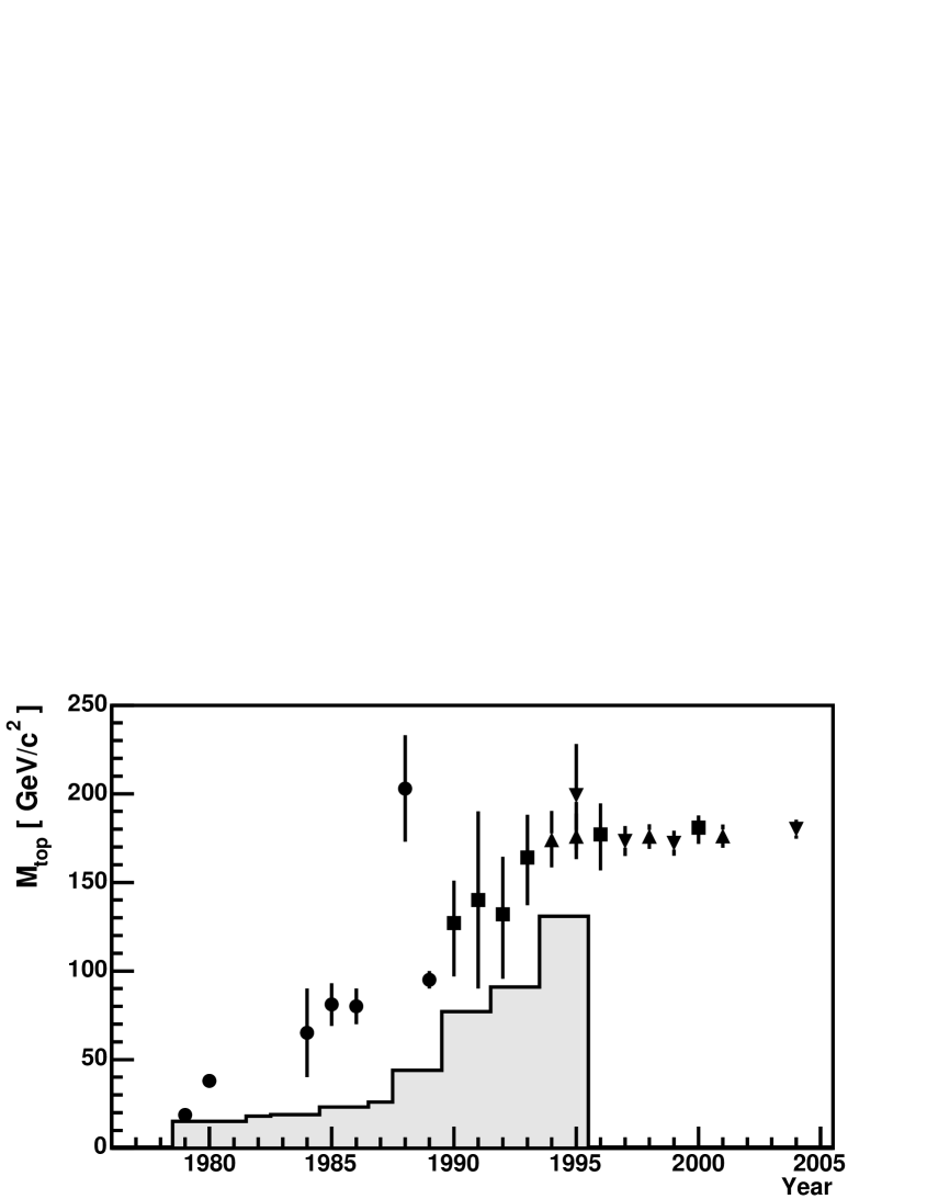
Figure 20: History of the quest for the top quark. The shaded histogram shows experimental lower limits on the top quark mass. Theoretical predictions based on flavour symmetries are shown (dots) as well as predictions based on electroweak precision measurements (squares). Direct measurements of $M_{\mathrm{top}}$ by CDF and DØ are represented by the triangle (triangles pointing up: CDF; triangles pointing down: DØ ).

A likelihood fit to the observed mass distribution yields a central value for the top quark mass of $M_{top}=199^{+19}_{-21}\;\mathrm{(stat.)}\pm 22\;\mathrm{(syst.)}\;\mathrm{GeV}/c^{2}$.

In September 1995 CDF completed the series of publications establishing the top quark discovery with a complementary kinematic analysis without $b$ tagging, that used the $E_{\mathrm{T}}$ of the second and third highest $E_{\mathrm{T}}$ jets to calculate a relative likelihood for each event to be top quark like or background like [208, 209]. The probability for the observed data to be due to a background fluctuation was found to be 0.26%.

Finally, 17 years after the discovery of the $b$ quark its weak isospin partner, the top quark, was firmly established. In figure 20 we summarise the long lasting quest for the top quark. The figure shows the lower experimental limits on the top quark mass (histogram) [186, 210, 211, 185, 212, 195, 198, 201, 203], theoretical predictions mainly based on flavour symmetries within the quark mass matrix (dots) [182, 213, 214, 215, 216, 217, 218] and predictions based on electroweak precision measurements at LEP and SLC (squares) [219, 220, 221, 48, 222, 223] as discussed in section 2.3. The direct measurements by CDF [204, 205, 224, 104] and DØ [207, 225, 226, 106] are also included (triangles). The good agreement between the measured top quark mass and the prediction obtained from electroweak precision measurements constituted a major success of the Standard Model.

6 $\mathbf{t\bar{t}}$ cross section measurements

Within the SM the $t\bar{t}$ cross section is calculated with a precision of about 15% [99, 91], see also section 3.1.4. The SM further predicts that the top quark decays to a $W$ boson and a $b$ quark with a branching ratio close to 100%. Measuring the cross section in all possible channels tests both, production and decay mechanisms of the top quark. A significant deviation from the SM prediction would indicate either the presence of a new production mechanism, e.g. a heavy resonance decaying into $t\bar{t}$ pairs, or a novel decay mechanism, e.g. into supersymmetric particles. The $t\bar{t}$ cross section depends sensitively on the top quark mass. In the mass interval of $170\leq M_{\mathrm{top}}\leq 190\,\mathrm{GeV}/c^{2}$ the cross section drops by roughly 0.2 pb for an increase of 1 GeV/$c^{2}$ in $M_{\mathrm{top}}$. This theoretically predicted dependence can be exploited to turn a cross section measurement into an indirect determination of the top quark mass. A 15% measurement of the cross section is approximately equivalent to a 3% measurement of $M_{\mathrm{top}}$. One can also turn the argument around and use the measurements of the cross section and the top quark mass and test their compatibility with the theoretically predicted cross section and its mass dependence as indicated in figure 9 in section 3.1.4.

The $t\bar{t}$ cross section measurements are very fundamental to top quark physics at the Tevatron, since these analyses isolate data samples that are enriched in $t\bar{t}$ events and lay thereby the foundations for further investigations of top quark properties. The $t\bar{t}$ cross section has been measured in the dilepton, the lepton-plus-jets and the all hadronic channel. So far the $t\bar{t}$ tau modes evaded observation. In this section we discuss the experimental methods applied in $t\bar{t}$ cross section measurements in more detail. We highlight representative Tevatron analyses for different channels and analyses methods, either from CDF or DØ. A comprehensive summary of all measurements and the combined cross section results is presented in section 6.4.

6.1 Dilepton channel

As mentioned in section 4.4 the dilepton channel comprises $t\bar{t}$ final states with two high $p_{\mathrm{T}}$ charged leptons (electrons or muons), $E_{\mathrm{T}}\!\!\!\!\!\!\!/\ \;$ and two $b$ quark jets. This clean signature allows to select a $t\bar{t}$ sample with high purity, reaching a signal to background ratio between 1.5 and 3 depending on the analysis. In 2004 CDF published its first $t\bar{t}$ cross section measurement at $\sqrt{s}=1.96\,\mathrm{TeV}$ in the dilepton channel based on a data sample with an integrated luminosity of $\mathcal{L}_{\mathrm{int}}=(197\pm 12)\,\mathrm{pb^{-1}}$ [227], i.e. about twice as much data as used in Run I. Two complementary analyses are performed. The first one requires both leptons to be specifically identified as either electrons or muons, while the second technique allows one of the leptons to be identified only as a high-$p_{\mathrm{T}}$ isolated track, thereby significantly increasing the lepton detection efficiency at cost of a moderate increase in the expected backgrounds. In the following we will concentrate the discussion on the second, the lepton-plus-track analysis.

At trigger level the data samples used in dilepton analyses are selected by finding events that either contain a central electron or muon candidate with $E_{\mathrm{T}}>18\;\mathrm{GeV}$, or an electron candidate in the forward calorimeter with $E_{\mathrm{T}}>20\;\mathrm{GeV}$ and $E_{\mathrm{T}}\!\!\!\!\!\!\!/\ \;>15\;\mathrm{GeV}$. In the offline analysis two oppositely charged leptons with $E_{\mathrm{T}}>20\;\mathrm{GeV}$ are required. One lepton, the “tight” lepton has to pass strict lepton identification criteria and be isolated. Tight electrons have a well measured track pointing at an energy deposition in the calorimeter. For electrons with $|\eta|>1.2$, this track association is made by a calorimeter-seeded silicon tracking algorithm. Tight muons must have a well-measured track linked to a track segment in the muon chambers and an energy deposition in the calorimeters consistent with that expected for muons. The second lepton, the “loose” lepton, is defined as a well-measured, isolated track with $p_{\mathrm{T}}>20\;\mathrm{GeV}/c$ and a pseudorapidity of $|\eta|<1.0$.

Candidate events must have a $E_{\mathrm{T}}\!\!\!\!\!\!\!/\ \;>25$ GeV. The value of $E_{\mathrm{T}}\!\!\!\!\!\!\!/\ \;$ is corrected for all loose leptons if the associated calorimeter $E_{\mathrm{T}}$ is less than 70% of the track $p_{\mathrm{T}}$. Events are rejected if the vector $\bi{E}_{\mathrm{T}}\!\!\!\!\!\!\!/\;\;$ lies within $5^{\circ}$ of the loose lepton axis and $E_{\mathrm{T}}\!\!\!\!\!\!\!/\ \;<50$ GeV. Jets are counted with a threshold of $E_{\mathrm{T}}>20\,\mathrm{GeV}$ and within the pseudorapidity range of $|\eta|<2.0$. At least two jets defined in that way are required. Candidates being compatible with cosmic ray muons or photon conversions are removed. To remove dilepton pairs due to $Z^{0}$ boson production the cut on the missing transverse energy is tightened to $E_{\mathrm{T}}\!\!\!\!\!\!\!/\ \;>40$ GeV in a window of $\pm 15\;\mathrm{GeV}/c^{2}$ around the $Z^{0}$ mass.

The dominant backgrounds to $t\bar{t}$ dilepton events are Drell-Yan ($q\bar{q}\rightarrow Z/\gamma^{*}\rightarrow\ell^{+}\ell^{-}$) production, misidentified (fake) leptons in $W\rightarrow\ell\nu+\mathrm{jets}$ events where one jet is falsely reconstructed as a lepton candidate, and diboson ($WW$, $WZ$, and $ZZ$) production. The Drell-Yan background is estimated by a combination of fully simulated Pythia Monte Carlo events and CDF data. A sample of $Z$ boson candidates in the mass range of 76 – 106 GeV/$c^{2}$ is selected. The numbers of events passing the nominal $t\bar{t}$ selection or a Drell-Yan specific selection are obtained, respectively. These two numbers provide the normalization for the expected Drell-Yan background contributions to the $t\bar{t}$ dilepton sample as obtained from Monte Carlo. The rate of lepton misidentification is obtained from an inclusive jet sample after removing sources of real leptons such as $W$ and $Z$ boson decays. The accuracy and robustness of the derived lepton fake rate is checked with several control samples and good agreement is found within the statistical uncertainties. The diboson background estimates are derived by calculating the acceptances from Monte Carlo and applying the theoretical cross sections which have a relatively small uncertainty. The total number of background events expected in the data sample is $6.9\pm 1.7$ of which 61% are due to Drell-Yan processes, 22% are due to fake leptons, and 17% are due to diboson production. CDF observes 18 events in data. The $t\bar{t}$ cross section is calculated according to the formula

$$\sigma(t\bar{t}\,)=\frac{N_{\mathrm{obs}}-N_{\mathrm{bkg}}}{\epsilon_{\mathrm{evt}}\cdot\mathcal{L}_{\mathrm{int}}}\ ,$$ (31)

where $N_{\mathrm{obs}}$ is the number of observed events, $N_{\mathrm{bkg}}$ is the number of expected background events, and $\epsilon_{\mathrm{evt}}$ is the event detection efficiency which includes the kinematic acceptance, trigger and reconstruction efficiencies, and the branching ratio into dilepton events. The event detection efficiency is $\epsilon_{\mathrm{evt}}=(0.88\pm 0.12)\%$, including a branching ratio of $\mathrm{BR}(W\rightarrow\ell\nu)=10.8\%$ for the $W$ boson decay into a charged lepton plus neutrino. The kinematic acceptance is evaluated for a top mass of $M_{\mathrm{top}}=175\,\mathrm{GeV}/c^{2}$. The resulting value of the cross section is $7.0^{+2.7}_{-2.3}\,(\mathrm{stat.})^{+1.5}_{-1.3}\,(\mathrm{syst.})\pm 0.4\;(\mathrm{lumi.})\,\mathrm{pb}$, which is in very good agreement with the theoretical prediction of $6.7^{+0.7}_{-0.9}\,\mathrm{pb}$ [91]. The distributions of various kinematic variables are found to be consistent with the SM prediction as obtained from Pythia Monte Carlo. As an example, the distribution of the scalar sum of all transverse energies in the event is shown in figure 22.

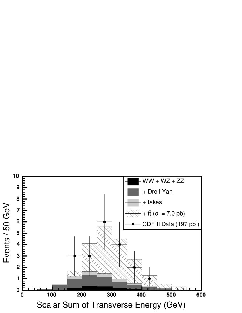
Figure 21: The scalar sum of all transverse energies in the event. The histograms are stacked. The shaded histograms are the backgrounds, the hatched histogram shows the $t\bar{t}$ signal distribution scaled to the measured cross section. The dots plus error bars are data from the first CDF $t\bar{t}$ dilepton analysis in Run II [227].

Figure 22: Scatter plots of aplanarity versus $H_{\mathrm{T}}$ for (a) the $W+4$ jets background sample, (b) QCD multijet background events, (c) $t\bar{t}$ Monte Carlo events from Herwig, and (d) DØ lepton plus jets data. The dashed lines represent the threshold values used for the selection in the DØ topological analysis [105].

A Kolmogorov-Smirnov test of this distribution yields a $p$-value of 75%.

6.2 Lepton-plus-jets channel

The signature of the $t\bar{t}$ lepton-plus-jets channel comprises a high-$p_{\mathrm{T}}$ electron or muon, missing transverse energy and four jets, see section 4.4. The branching fraction of this channel is about 30% which is one of the advantages over the dilepton channel. However, $W+\mathrm{multijet}$ backgrounds are large and call for dedicated strategies to improve the signal to background ratio. In this section we discuss four important methods to reduce backgrounds in the lepton-plus-jets channel and obtain a measurement of the $t\bar{t}$ cross section.

6.2.1 Topological analyses

The production of two very heavy objects in $t\bar{t}$ events is reflected in several kinematic distributions that describe the general event topology. Some analyses take advantage of the fact that the scalar sum of transverse energies, $H_{\mathrm{T}}$, tends to be much higher in $t\bar{t}$ events than in background events. This is due to the fact that jets originating from the decay of a heavy object are typically much harder, i.e. higher in $E_{\mathrm{T}}$, than those from gluon radiation. Other analyses utilise the higher spherical symmetry of $t\bar{t}$ events. More recent analyses combine several kinematic variables into one kinematic discriminant using a neural network [228].

We discuss here in more detail the final DØ topological analysis used to measure the $t\bar{t}$ cross section in Run I at $\sqrt{s}=1.8\,\mathrm{TeV}$ [105]. This analysis marks the final result of the technique used in DØ to discover the top quark in the lepton-plus-jets channel in 1995 [207]. The data were selected by a lepton-plus-jets trigger, requiring one loosely identified electron or muon and at least one jet. The electron data set corresponds to a luminosity of 119.5 $\mathrm{pb^{-1}}$, the muon data set to 107.7 $\mathrm{pb^{-1}}$. The offline selection asks for an isolated, well identified electron with $E_{\mathrm{T}}>20\,\mathrm{GeV}$ and $|\eta|\leq 2.0$ or an isolated, well identified muon with $p_{\mathrm{T}}>20\,\mathrm{GeV}/c$ and $|\eta|\leq 1.7$. The missing transverse energy as calculated in the calorimeter has to be above 25 GeV for electron-plus-jets events and above 20 GeV for muon-plus-jets events. The pseudorapidity of the reconstructed $W$ boson is required to be $|\eta(W)|\leq 2.0$. Jets are counted with a threshold of $E_{\mathrm{T}}>15\,\mathrm{GeV}$ and $|\eta|<2.0$. Events with four or more jets are accepted. To avoid an overlap with the soft muon $t\bar{t}$ analysis events with jets having a soft muon $b$ tag are excluded.

Three topological variables are used to further discriminate between signal and background: (1) the $H_{\mathrm{T}}$ variable which is defined as the scalar sum of all transverse jet energies using the jet definition as mentioned above, (2) the scalar sum of $E_{\mathrm{T}}\!\!\!\!\!\!\!/\ \;$ and the lepton $p_{\mathrm{T}}$ which is denoted $E_{\mathrm{T}}^{\mathrm{L}}$, and (3) the aplanarity $\mathcal{A}$ which is an event shape variable quantifying the “flatness” of an event and is defined as $\frac{3}{2}$ times the smallest eigenvalue of the normalized laboratory momentum tensor $\mathcal{M}$ of the observed physics objects. The tensor $\mathcal{M}$ is defined by:

$$\mathcal{M}_{ij}=\frac{\sum_{k}p_{ki}\,p_{kj}}{\sum_{k}|\bi{p}_{k}|^{2}}$$ (32)

where $\bi{p}_{k}$ is the three momentum of the object $k$ and the indices $i$ and $j$ are the $x$, $y$ and $z$ coordinates. The sum runs over all objects under consideration, i.e. all jets defined by the cuts $E_{\mathrm{T}}>15\,\mathrm{GeV}$ and $|\eta|<2.0$, and the $W$ boson reconstructed from the lepton and $\bi{E}_{\mathrm{T}}\!\!\!\!\!\!\!/\;\;$. Large values of $\mathcal{A}$ are indicative of spherical events, whereas small values correspond to more planar events. The following cuts on topological variables are used: $H_{\mathrm{T}}>180\,\mathrm{GeV}$, $E_{\mathrm{T}}^{\mathrm{L}}>60\,\mathrm{GeV}$ and $\mathcal{A}>0.065$. These cuts result from an optimization procedure such that the smallest error on the measured cross section and the best signal to background ratio $S/B$ are achieved.

The main backgrounds to the topological $t\bar{t}$ analysis arise from $W+\mathrm{jets}$ events and QCD multijet events that contain a misidentified electron or an isolated muon and mismeasured $E_{\mathrm{T}}\!\!\!\!\!\!\!/\ \;$. The background estimate proceeds in three major steps. In a first step the QCD multijet background is estimated as a function of jet multiplicity from data samples where all selection cuts except the three topological cuts are applied. The electron and the muon samples are treated separately because processes that give rise to a misidentified electron or an isolated muon are significantly different.

Jets that produce showers with a large fraction of the energy in the electromagnetic calorimeter can sometimes pass the electron selection criteria and be falsely identified as an electron. To determine the rate of multijet events containing such misidentified electrons one examines the $E_{\mathrm{T}}\!\!\!\!\!\!\!/\ \;$ spectrum of events that pass the electron trigger but fail the full offline electron identification. These events correctly describe the shape of the $E_{\mathrm{T}}\!\!\!\!\!\!\!/\ \;$ distribution of QCD multijet events, while the normalization has to be found by matching the number of events at low $E_{\mathrm{T}}\!\!\!\!\!\!\!/\ \;$ between this background sample and the sample where the full electron identification has been applied. The number of events in the tail of the normalized distribution above $E_{\mathrm{T}}\!\!\!\!\!\!\!/\ \;>25\,\mathrm{GeV}$ provides an estimate on the number of QCD multijet background events.

Muons from semileptonic $b$ of $c$ quark decays are normally within a jet, i.e. they are nonisolated. However, occasionally the decay kinematics is such, that there is insufficient hadronic energy to produce a jet. In this case the muons from heavy quark decays appear to be isolated and constitute the major source of QCD multijet background in the muon-plus-jets sample. The rate of isolated muons from heavy quark decays is measured using multijet samples with $E_{\mathrm{T}}\!\!\!\!\!\!\!/\ \;<20\,\mathrm{GeV}$.

The multijet background is estimated for each inclusive $W+\mathrm{jet}$ multiplicity sample. In the $e+\geq 4\;\mathrm{jets}$ sample the background is estimated to be $7.2\pm 2.2$ events, in the $\mu+\geq 4\;\mathrm{jets}$ sample $13.9\pm 4.4$ events.

In the second step of the background estimate the rate of $W+\mathrm{multijet}$ events is computed using a fit to the jet multiplicity spectrum that remains after the subtraction of the QCD multijet background. This method exploits a simple exponential relationship between the number of events and the jet multiplicity

$$\frac{\sigma(W+n\ \mathrm{jets})}{\sigma(W+(n-1)\ \mathrm{jets})}=\alpha\ ,$$ (33)

where $\alpha$ is a constant that depends on the specific jet definition, i.e. the clustering algorithm as well as the $E_{\mathrm{T}}$ and $\eta$ requirements. Relation (33) is known as “Berends scaling” [229, 230] and based on the assumption that the observed jets come from gluon radiation where the emission of each additional jet is suppressed by a factor of the strong coupling constant $\alpha_{s}$. A fit to the observed DØ data yields a scaling parameter of $\alpha=0.18\pm 0.01$ for electron data and $\alpha=0.19\pm 0.02$ for muon data. These fit values are used to predict the number of background events in the $W+\geq 4$ jets sample and are found to be $44.8\pm 8.6$ events for electron-plus-jets events and $25.8\pm 4.6$ events for the muon-plus-jets sample. As a side remark it has to be noted that $\alpha$ cannot simply be identified with $\alpha_{s}$, since the variation of $\alpha_{s}$ in the PDFs has to be taken into account [231]. If this is properly done the sensitivity to $\alpha_{s}$ is largely lost.

In the third step the cut efficiencies for the topological cuts are computed and then applied to the previously derived background estimate for the $W+\geq 4$ jets sample. The efficiency on the QCD multijet background is again derived from data, while the efficiency on the $W+\mathrm{jets}$ background is taken from events generated with the Vecbos Monte Carlo program [177]. After applying all cuts the total background is predicted to be $4.51\pm 0.91$ in the $e+\geq 4$ jets sample and $4.32\pm 1.04$ events in the $\mu+\geq 4$ jets sample, while 9 or 10 events are observed in data, respectively.

The event detection efficiency $\epsilon_{\mathrm{evt}}$ for the $t\bar{t}$ signal is determined from Herwig Monte Carlo events that were passed through the DØ detector simulation. For a top quark mass of $M_{\mathrm{top}}=170\,\mathrm{GeV}/c^{2}$ a value of $\epsilon_{\mathrm{evt}}=(1.29\pm 0.23)\%$ is found for the electron sample, and $\epsilon_{\mathrm{evt}}=(0.91\pm 0.27)\%$ for the muon sample. Using $\epsilon_{\mathrm{evt}}$ determined for a top mass of $M_{\mathrm{top}}=172.1\,\mathrm{GeV}/c^{2}$ as measured by DØ the cross section is computed to be $(2.8\pm 2.1)\,\mathrm{pb}$ in the electron-plus-jets channel and $(5.6\pm 3.7)\,\mathrm{pb}$ in the muon-plus-jets channel. Figure 22 shows the aplanarity versus $H_{\mathrm{T}}$ plane for the background samples, $t\bar{t}$ Monte Carlo and DØ data. The plots illustrate the effectiveness of reducing the background via the cuts on the topological variables $H_{\mathrm{T}}$ and $\mathcal{A}$.

6.2.2 Secondary vertex tag

While each $t\bar{t}$ event features two $b$ quark jets, only about 2% of the $W+\mathrm{jets}$ background contain a $b$ quark. Therefore, the $t\bar{t}$ signal can be significantly enhanced by identifying $b$ quark jets. Three different $b$ jet identification methods are discussed in section 4.5.4. In CDF the secondary vertex tagging method proved to be the most effective one, yielding the cross section measurement with the smallest total uncertainty.

We present here a summary of the first CDF Run II $t\bar{t}$ cross section measurement using lepton-plus-jets events with secondary vertex $b$ tagging [168]. The $b$ tagging method has already been presented in section 4.5.4. That is why we concentrate here on the event selection and the background estimate. The analysis uses a data sample triggered by high momentum electrons or muons corresponding to an integrated luminosity of 162 $\mathrm{pb^{-1}}$. The electron selection requires an isolated cluster in the central calorimeter with $E_{\mathrm{T}}>20\,\mathrm{GeV}$ matched to a track with $p_{\mathrm{T}}>10\,\mathrm{GeV}/c$. Muon candidates have a track in the drift chamber with $p_{\mathrm{T}}>20\,\mathrm{GeV}/c$ that is matched to a track segment in the muon chambers. Events consistent with being photon conversions (electrons) or cosmic rays (muons) are rejected. The missing transverse energy is required to be $E_{\mathrm{T}}\!\!\!\!\!\!\!/\ \;>20\,\mathrm{GeV}$. By requiring one and only one well identified lepton $t\bar{t}$ dilepton events and $Z\rightarrow e^{+}e^{-}/\mu^{+}\mu^{-}$ events are suppressed. To improve the removal efficiency for $Z$ bosons, events are also removed if a second, less stringently identified lepton is found that forms an invariant mass $M_{\ell\ell}$ with the primary lepton within the window of $76<M_{\ell\ell}<106\,\mathrm{GeV}/c^{2}$. Jets are defined as clusters in the hadronic calorimeter with $E_{\mathrm{T}}>15\,\mathrm{GeV}$ and $|\eta|<2.0$. At least three jets are required for an event to fall into the signal region. One of these jets has to be identified as containing a $b$ quark using the secondary vertex tag algorithm. The final cut is on the total transverse energy and demands $H_{\mathrm{T}}>200\,\mathrm{GeV}$, which rejects approximately 40% of the background while retaining 95% of $t\bar{t}$ signal events.

The secondary vertex tag algorithm is described in section 4.5.4. Figure 17a shows the distribution of the two-dimensional decay length of secondary vertices in the CDF data sample compared to the SM prediction of $t\bar{t}$ signal and background. Good agreement is found. The backgrounds to the secondary vertex tagged sample are (i) direct QCD production of heavy flavour quarks without an associated $W$ boson (non-$W$ QCD), (ii) $W$ plus light quark jets events where one jet is falsely identified as heavy flavour (mistags), (iii) $W$ plus heavy flavour jets, (iv) diboson production, single top quark, and $Z\rightarrow\tau^{+}\tau^{-}$ production. The estimate of these backgrounds is partially derived from CDF data and partially from Monte Carlo. In particular, the number of $b$ tagged $W+\mathrm{jets}$ background events is calibrated with the number of observed $W+\mathrm{jets}$ events before $b$ tagging. Therefore, the first step in the background calculation is to estimate the number of background events that do not contain a $W$ boson in the pretag sample and subtract that background from the observed number of events.

(i) Non-W QCD background: The non-$W$ background is mainly due to events where a jet is misidentified as an electron and the $E_{\mathrm{T}}\!\!\!\!\!\!\!/\ \;$ is mismeasured, or due to muons from semileptonic $b$ decays which pass the isolation criterion. Since the background sources in the electron and muon sample are different, one has to treat these two samples separately. The non-$W$ background estimate uses the $E_{\mathrm{T}}\!\!\!\!\!\!\!/\ \;$ variable and the isolation variable $R_{\mathrm{iso}}$, that is defined as the ratio of calorimeter energy $E_{\mathrm{iso}}$ contained in an isolation annulus of $\Delta R=0.4$ around the lepton (excluding the energy associated to the lepton) divided by the lepton energy $E_{\ell}$. The $R_{\mathrm{iso}}$ versus $E_{\mathrm{T}}\!\!\!\!\!\!\!/\ \;$ plane is divided into a signal region ($R_{\mathrm{iso}}<0.1$ and $E_{\mathrm{T}}\!\!\!\!\!\!\!/\ \;>20\,\mathrm{GeV}$) and three sideband regions. One assumes that the two variables are uncorrelated for non-$W$ background events and calculates the number of background events in the signal region as a simple proportion of events in the sideband regions. The contribution of true $W$ and $t\bar{t}$ events in the sideband regions is subtracted using Monte Carlo predictions normalized to the observed number of events in the signal region. In the pretag $e+\geq 3$ jets sample $(20\pm 5)\%$ of the events are estimated to be non-$W$ events, in the $\mu+\geq 3$ jets sample it is $(7.5\pm 2.3)\%$. The pretag sample is defined as the data sample where all selection cuts have been applied except requiring a $b$ tag. In the final sample, after requiring a secondary vertex tag, about 18% of the total background is due to non-$W$ events.

(ii) Mistags: The mistag rate of the secondary vertex algorithm is measured using inclusive jet samples. Mistags are caused mostly by a random combination of tracks which are displaced from the primary vertex due to tracking errors. The main idea is to use the rate of events with negative two-dimensional decay length as an estimate of the mistag rate. Corrections due to material interactions, long-lived light flavour particles (e.g. $K_{s}^{0}$ and $\Lambda$), and negatively tagged heavy flavour jets are determined using fits to the effective lifetime spectra of tagged vertices. The mistag rate is parameterized as a function of four jet variables: $E_{\mathrm{T}}$, the good track multiplicity, $\eta$ and $\phi$ of the jet as well as one event variable, i.e. the scalar sum of the $E_{\mathrm{T}}$ of all jets with $E_{\mathrm{T}}>8\,\mathrm{GeV}$. To estimate the mistag background in the $W+\mathrm{jets}$ sample each jet in the pretag sample is weighted with its mistag rate. The sum of weights over all jets in the sample is then scaled down by the fraction of non-$W$ events in the pretag sample. Since the mistag rate per jet is sufficiently low, this prediction of mistagged jets is a good estimate on the number of events with a mistagged jet. It is found that 34% of the background for the final $t\bar{t}$ selection are due to mistags.

(iii) W + heavy flavour: The production of a $W$ boson in association with heavy flavour quarks is the main background to the $t\bar{t}$ signal with a secondary vertex tag. Heavy quarks occur in the process $q_{1}\bar{q}_{2}\rightarrow W+g$ where the gluon splits into a $b\bar{b}$ or a $c\bar{c}$ pair, and in the process $gq\rightarrow Wc$. As mentioned in section 4.6, the Alpgen Monte Carlo program [178] is used to generate several samples of exclusive $W+n\;\mathrm{jets}$ final states. This includes $W+b\bar{b}/c\bar{c}+n$ jets, and $Wc+\mathrm{jets}$. The Alpgen generation is followed by showering with Herwig. To reproduce the entire $W+\mathrm{multijets}$ spectrum the exclusive samples are merged together taking the appropriate cross sections into account. The combination procedure avoids double counting of jets produced at matrix element level with Alpgen and hard jets produced by the showering in Herwig. A jet clustering algorithm is run at Monte Carlo particle level after showering but before detector simulation. These Monte Carlo jets are matched to partons generated at matrix element level. If extra jets occur, that do not match a parton, the event is rejected.

While the shape of the $W+n\;\mathrm{jets}$ spectrum can be reproduced well by the Monte Carlo, the absolute normalization has large theoretical uncertainties and is therefore taken from collider data. The heavy flavour fractions predicted by Alpgen are found to be too small and are calibrated against fractions measured in inclusive jet data. The composition of the inclusive jet sample is determined by fitting the pseudo-$c\tau$ distribution for $b$ tagged jets. The pseudo-$c\tau$ is defined as $L_{\mathrm{2D}}\cdot M_{\mathrm{vtx}}/p_{\mathrm{T}}^{\mathrm{vtx}}$, where $L_{\mathrm{2D}}$ is the two-dimensional decay length (see also section 4.5.4), $M_{\mathrm{vtx}}$ is the invariant mass of all tracks associated to the secondary vertex, and $p_{\mathrm{T}}^{\mathrm{vtx}}$ is the transverse momentum of the vertex 4-vector. Figure 23a shows the pseudo-$c\tau$ distribution for the inclusive jet data as well as the fitted heavy flavour components.

(a)                                                        (b)

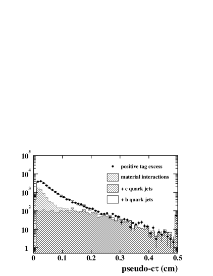
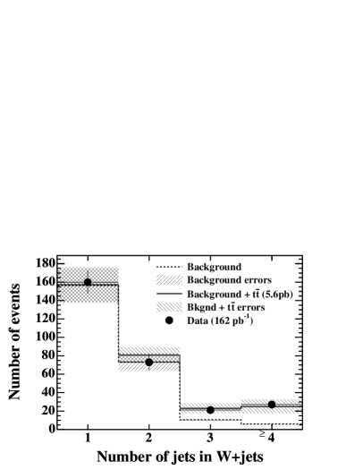
Figure 23: (a) Pseudo-$c\tau$ distribution for inclusive jet data. The distribution is used to measure the heavy flavour fractions in the jet sample. The fitted contributions for the different heavy flavour components and secondary interactions in light flavour jets are shown [168]. (b) Jet multiplicity spectrum for CDF data (dots), the total background expectation (dashed histogram), and the sum of background and the predicted $t\bar{t}$ signal ($\sigma=6.7\,\mathrm{pb}$, full line).

The template distributions for heavy flavour jets used in the fit are taken from Alpgen Monte Carlo samples. The measured heavy flavour fractions in jet data are consistently higher by 50% than the Alpgen prediction. Therefore, a correction factor of $1.5\pm 0.4$ is applied to the heavy flavour fractions in the $W+\mathrm{multijets}$ sample. The assumption here is that this correction factor is universal and can be transferred from the inclusive jets to the $W+\mathrm{multijets}$ sample. As a result, it is found, that the fraction of $W+4$ jets events coming from the $Wb\bar{b}$ process is $(4.8\pm 1.3)\%$, the fraction with one or two $c$ jets from $Wc\bar{c}$ is $(7.3\pm 2.0)\%$, and the fraction of $Wc$ events is $(6.1\pm 1.3)\%$. It has to be noted that the $Wc$ fraction is directly taken from the Alpgen prediction and is not corrected, since it is due to a different physics process.

The number of $W+$ heavy flavour background events for the $t\bar{t}$ analysis is computed by multiplying the derived heavy quark fractions by the number of pretag events, after subtracting the non-$W$ background. The heavy flavour contributions to the total background in the $t\bar{t}$ candidate sample are as follows: 25% are due to $Wb\bar{b}$, 8% due to $Wc\bar{c}$ and 6% due to $Wc$ production.

(iv) Diboson, single top and $Z\rightarrow\tau^{+}\tau^{-}$: There is a number of smaller backgrounds which can be reliably predicted by combining the event detection efficiency for these processes as determined from Monte Carlo events with the theoretically predicted cross section. This method is feasible, since the cross section predictions for diboson production processes, i.e. $WW$, $WZ$ and $ZZ$, and single top quark production have relatively small uncertainties. Diboson events can mimic a $t\bar{t}$ signal if one boson decays leptonically and the other one decays into jets, where at least one jet is due to a $b$ or $c$ quark. In addition, $Z+\mathrm{jet}$ production can mimic $t\bar{t}$ events if the $Z$ boson decays into $\tau^{+}\tau^{-}$ and one $\tau$ decays leptonically producing an isolated electron or muon, while the second $\tau$ decays hadronically. The contribution of diboson, $Z\rightarrow\tau^{+}\tau^{-}$ and single top events to the total background is found to be 9%.

The total background prediction is $13.5\pm 1.8$ events, while 48 events are observed in the $W+\geq 3$ jets sample. The clear excess of events is attributed to $t\bar{t}$ production. Figure 23b shows the jet multiplicity spectrum for CDF data, the total background expectation, and the sum of background and the predicted $t\bar{t}$ signal. A very good agreement between the data and the SM expectation is found.

To compute the $t\bar{t}$ cross section according to (31), the event detection efficiency $\epsilon_{\mathrm{evt}}$ for $t\bar{t}$ events is needed. It is obtained from a sample of Pythia $t\bar{t}$ Monte Carlo events. The trigger efficiency as well as several correction factors that account for differences between data and Monte Carlo events are measured with control data samples. Particularly important is the correction factor for the $b$ tagging efficiency. A sample of inclusive electrons with $p_{\mathrm{T}}>7\,\mathrm{GeV}$ is used for this purpose. Many electrons in this momentum regime originate from semileptonic $b$ decays. Therefore, the sample is enriched in heavy flavour. Using a double tag technique it is found that the average tagging efficiency of a $b$ quark jet in data is $(24\pm 1)\%$, while the Monte Carlo predicts $(29\pm 1)\%$, thus yielding a $b$ tagging correction factor of $0.82\pm 0.06$, where the error includes systematic uncertainties. The efficiency to tag at least one jet in a $t\bar{t}$ event, after all other cuts have been applied, is found to be $(53.4\pm 3.2)\%$. The uncertainty is almost purely systematic. The overall event detection efficiency is $\epsilon_{\mathrm{evt}}=(3.84\pm 0.40)\%$. This yields a cross section measurement of $\sigma(t\bar{t})=5.6^{+1.2}_{-1.1}\,(\mathrm{stat.})\,^{+0.9}_{-0.6}\,(\mathrm{syst.})\,\mathrm{pb}$, which is in good agreement with the theoretical expectation of $6.7^{+0.7}_{-0.9}\,\mathrm{pb}$. The statistical uncertainty is larger than the systematic one, but very soon, using more data, the systematic uncertainty will start to dominate the measurement. Although, having larger control samples at hand, it will be possible to also reduce the systematic uncertainty.

6.2.3 Impact parameter tag

The impact parameter $b$ tagging algorithm is an alternative method to identify $b$ quark jets. The method also relies on the long lifetime of $b$ hadrons, but the explicit reconstruction of a secondary vertex is not required. The algorithm rather asks for tracks with high impact parameter significance and is explained in section 4.5.4. In the CDF Run II analysis presented here a jet is $b$ tagged if its probability to be consistent with a zero lifetime hypothesis is below 0.01 [232]. The $b$ tagging efficiency of the algorithm is measured in inclusive electron data using a double tag method. For heavy flavour jets with $E_{\mathrm{T}}>10\,\mathrm{GeV}$ the average tagging efficiency is found to be $(19.7\pm 1.2)\%$.

The event selection for the $t\bar{t}$ cross section measurement is essentially the same as described in section 6.2.2 for the analysis using a secondary vertex $b$ tag. There is one additional cut which requires that the $\Delta\phi$ between the $\bi{E}_{\mathrm{T}}\!\!\!\!\!\!\!/\;\;$ and the most energetic jet is within $[0.5,2.5]$ radians if $E_{\mathrm{T}}\!\!\!\!\!\!\!/\ \;<30\,\mathrm{GeV}$. The cut on $H_{\mathrm{T}}$ is omitted. The background is estimated based on the same techniques as the measurement using the secondary vertex tag. The mistag rate of light quark jets is measured in an inclusive jet data sample and found to be $(1.11\pm 0.06)\%$. In a data sample corresponding to $162\,\mathrm{pb^{-1}}$ 59 $W+\geq 3$ jets events are observed after all cuts, while the total background is estimated to be $24.7^{+4.8}_{-4.6}$ events. The overall event detection efficiency is found to be $\epsilon_{\mathrm{evt}}=(4.09\pm 0.61)\%$ which includes the event $b$ tagging efficiency of $(57.2\pm 3.9)\%$. As a result, the $t\bar{t}$ cross section is calculated to be $\sigma(t\bar{t})=5.8^{+1.3}_{-1.2}\,(\mathrm{stat.})\pm 1.3\,(\mathrm{syst.})\,\mathrm{pb}$, which is in good agreement with the result obtained with the secondary vertex $b$ tagging algorithm.

6.2.4 Soft lepton tag

The third technique to identify $b$ quark jets searches for electrons or muons within jets originating from semileptonic $b$ decays. We present here a CDF analysis using a soft muon tag [233]. A data sample with an integrated luminosity of 194 $\mathrm{pb^{-1}}$ is used. The event selection before $b$ tagging is the same as for the secondary vertex tag analysis. After all cuts 337 events are retained.

The soft muon tag algorithm uses a global $\chi^{2}$ built from several characteristic distributions that separate muon candidates from background. A jet is considered as $b$ tagged if it contains a muon with $p_{\mathrm{T}}>3\,\mathrm{GeV}/c$ and $\chi^{2}<3.5$ within $\Delta R<0.6$ of the jet axis. Events are rejected if the isolated high $p_{\mathrm{T}}$ lepton is a muon of opposite charge to the soft muon and the dimuon invariant mass is consistent with a $J/\psi$, an $\Upsilon$ or a $Z^{0}$. The efficiency to tag a $t\bar{t}$ event is approximately 15%, with small variations between the $W+3$ jets and $W+4$ jets samples. The rate of background events where a light quark jet is misidentified as containing a semileptonic $b$ hadron decay is estimated from a sample of photon-plus-jets events. The misidentification probability of a track with $p_{\mathrm{T}}>3\,\mathrm{GeV}/c$ and $\Delta R<0.6$ is found to be about 0.7%.

In the $W+\geq 3$ jets data sample 20 events with a soft muon tag are found, while the total expected background is estimated to be $9.5\pm 1.1$ events. The total event detection efficiency is $\epsilon_{\mathrm{evt}}=(1.0\pm 0.1)\%$ and the resulting $t\bar{t}$ cross section is found to be $\sigma(t\bar{t})=5.3\pm+3.3\,(\mathrm{stat.})\,^{+1.3}_{-1.0}\,(\mathrm{syst.})\,\mathrm{pb}$.

6.3 All hadronic channel

While the all hadronic channel has the largest branching ratio of all $t\bar{t}$ event categories, the QCD multijet background is overwhelming and it is therefore very challenging to isolate a $t\bar{t}$ signal. We present here a DØ analysis based on a Run II dataset corresponding to 162 $\mathrm{pb^{-1}}$ [234]. To enrich the signal content secondary vertex $b$ tagging and a multivariate analysis with artificial neural networks is employed.

The data sample is collected with a dedicated jet trigger at an average trigger efficiency of 74%. The event pre-selection asks for six or more jets, that are reconstructed with an algorithm using a fixed cone radius of $\Delta R=0.5$. Jets are counted with $E_{\mathrm{T}}>15\,\mathrm{GeV}$ and $|\eta|<2.5$. Events that contain an isolated lepton are rejected to obtain a dataset orthogonal to the lepton-plus-jets analysis. The reconstruction of secondary vertices is used to identify $b$ quark jets. A jet is considered to be tagged if a vertex with signed decay length significance larger than 7.0 is found. Exactly one $b$ tagged jet is required. Double tagged events are rejected to ease the background estimation. The efficiency to tag exactly one jet in a hadronic $t\bar{t}$ event is determined to be 46%.

The multivariate analysis combines 13 kinematic or event shape variables using two neural networks. The background sample for training the networks is obtained from the pretag data sample. A parametrization of the tagging rate is used to select events that have high probability to be tagged, but do in fact not have a tag. This ensures on one hand that the background sample is similar to the tagged events, but on the other hand is disjoint to the candidate sample. Signal Monte Carlo events are generated with Alpgen in combination with Pythia for showering and hadronization. After all cuts 220 candidate events are observed over a total background of $186\pm 5$ events. The event detection efficiency is $\epsilon_{\mathrm{evt}}=(2.8\pm 0.8)\%$ including a hadronic branching ratio of 46.19%. The $t\bar{t}$ production cross section is measured to be $\sigma(t\bar{t})=7.7^{+3.4}_{-3.3}\,(\mathrm{stat.})^{+4.7}_{-3.8}\,(\mathrm{syst.})\pm 0.5\,(\mathrm{lumi.})\;\mathrm{pb}$.

6.4 Cross section combination

In this section we summarise the final Run I $t\bar{t}$ cross section measurements and give a brief overview on the status of the currently available Run II measurements. The measured cross sections are presented in table 8.

Table 8: Measurements of the $t\bar{t}$ cross section at the Tevatron. The CDF measurements assume a top quark mass of $M_{\mathrm{top}}=175\,\mathrm{GeV}/c^{2}$ [103, 235, 236], the DØ measurements use $M_{\mathrm{top}}=172.1\,\mathrm{GeV}/c^{2}$ [105]. In Run II a top mass of $M_{\mathrm{top}}=175\,\mathrm{GeV}/c^{2}$ is assumed for the measurements of both experiments. The DØ Run I lepton-plus-jets cross section is a combination of the topological analysis and the soft lepton tag analysis. The given uncertainties include statistical and systematic contributions.

	Run I at $\sqrt{s}=1.8\,\mathrm{TeV}$		Run II at $\sqrt{s}=1.96\,\mathrm{TeV}$
Channel	CDF	DØ	CDF	DØ
Dilepton	$8.4^{+4.5}_{-3.5}\;\mathrm{pb}$	$6.0\pm 3.2\;\mathrm{pb}$	$7.0^{+2.9}_{-2.4}\;\mathrm{pb}$	$14.3^{+5.8}_{-4.8}\;\mathrm{pb}$
with secondary vertex tag				$11.1^{+6.0}_{-4.6}\;\mathrm{pb}$
global kinematic fit			$8.6^{+2.7}_{-2.6}\;\mathrm{pb}$
Lepton + jets		$5.1\pm 1.9\;\mathrm{pb}$
with secondary vertex tag	$5.1\pm 1.5\;\mathrm{pb}$		$5.6^{+1.5}_{-1.3}\;\mathrm{pb}$	$8.6^{+1.7}_{-1.6}\;\mathrm{pb}$
with impact parameter tag			$5.8\pm 1.8\;\mathrm{pb}$	$7.6^{+1.8}_{-1.5}\;\mathrm{pb}$
with soft lepton tag	$9.2\pm 4.3\;\mathrm{pb}$		$5.2^{+3.2}_{-2.1}\;\mathrm{pb}$
with $b$-tag and kinematic fit			$6.0\pm 2.0\;\mathrm{pb}$
with neural networks			$6.6\pm 1.9\;\mathrm{pb}$
All hadronic	$7.6^{+3.5}_{-2.7}\;\mathrm{pb}$	$7.3\pm 3.2\;\mathrm{pb}$	$7.5^{+3.9}_{-3.1}\;\mathrm{pb}$	$7.7^{+5.8}_{-5.1}\;\mathrm{pb}$
Combined	$6.5^{+1.7}_{-1.4}\,\mathrm{pb}$	$5.7\pm 1.6\;\mathrm{pb}$
Predicted [91]	$5.2^{+0.5}_{-0.7}\;\mathrm{pb}$		$6.7^{+0.7}_{-0.9}\;\mathrm{pb}$

For Run I the cross sections obtained from combination of all $t\bar{t}$ event categories for CDF and DØ are also shown [103, 105]. The combined values should be compared to the predicted cross section. Within the uncertainties good agreement is found.

In Run II various new techniques to measure the $t\bar{t}$ cross section are introduced. While the traditional dilepton analysis uses two leptons that meet strict identification criteria, CDF added an analysis where the identification of the second lepton is relaxed to increase the acceptance and reduce the statistical uncertainty. This analysis is discussed in more detail in section 6.1. Table 8 quotes the combined value for both CDF dilepton analyses [227]. A third CDF dilepton analysis uses a kinematic fit to the $(E_{\mathrm{T}}\!\!\!\!\!\!\!/\ \;,N_{\mathrm{jet}})$ phase space to disentangle the major SM processes contributing to the dilepton sample (global kinematic fit) [237]. DØ has made cross section measurements in a dilepton data sample without $b$ tagging [238] and in a $e\mu$ sample using a secondary vertex tag [239].

The CDF lepton-plus-jets analyses using three different $b$ tagging algorithms are presented in section 6.2. Based on a data set corresponding to $230\,\mathrm{pb^{-1}}$ the DØ collaboration has also presented measurements using a secondary vertex $b$ tag and an impact parameter tag [240]. CDF has performed two analyses that exploit kinematic properties of $t\bar{t}$ lepton-plus-jets events. One analysis uses the sample with secondary vertex tags and adds a likelihood fit to the transverse energy of the leading jet [241]. The second analysis is based on the $W+\geq 3$ jets sample before $b$ tagging and uses a neural network to construct a powerful discriminant between the backgrounds and the $t\bar{t}$ signal [228].

The DØ measurement of the $t\bar{t}$ cross section in the all hadronic channel [234] is discussed in section 6.3. The CDF Run II analysis in the all hadronic channel is similar to the DØ one, also requiring a secondary vertex $b$ tag and exploiting several kinematic variables [242]. But CDF uses simple sequential cuts rather than a multivariate combination via a neural network. At present, combined results on the $t\bar{t}$ cross section in Run II are not yet available. The combination of the different $t\bar{t}$ event categories (dilepton, lepton-plus-jets, all hadronic) is relatively straight forward, since the data sets are essentially orthogonal. However, the different analyses within a particular category are correlated, sometimes even strongly correlated. The correlation has to be determined and taken into account when a combination of the different analyses is done.

7 Top quark mass measurements

As discussed in section 2.3, the top quark mass is a very important parameter for the description of electroweak processes and precision tests of the SM. The main implication is that the SM relates the masses of the top quark, the $W$ boson and the Higgs boson, such that precise measurements of $M_{\mathrm{top}}$ and $M_{W}$ imply a prediction for $M_{H}$. Therefore, the precise measurement of the top quark mass is one of the major goals of Run II at the Tevatron. However, since Run II results on the top quark mass are not yet published, we describe in this chapter the two main methods used by CDF and DØ in Run I to determine $M_{\mathrm{top}}$: (1) the template method of CDF, which fits template distributions for different top quark masses to the distribution observed in data, and (2) the matrix element method of DØ, which exploits the sensitivity of the leading order matrix element for $t\bar{t}$ production to $M_{\mathrm{top}}$. Both methods are also used in Run II to measure $M_{\mathrm{top}}$. In section 7.3 we discuss the combination of top quark mass measurements in different $t\bar{t}$ event categories and among the two Tevatron experiments.

7.1 Template method in $t\bar{t}$ lepton-plus-jets events

The best measurement of the top quark mass is achieved in the $t\bar{t}$ lepton-plus-jets channel, since it features a relatively high number of candidate events, moderate background levels and allows for a full reconstruction of top quark momenta with reasonable accuracy. That is why we present here the final top quark mass measurement in lepton-plus-jets events at CDF in Run I [104]. The data sample used in the analysis corresponds to an integrated luminosity of 106 $\mathrm{pb^{-1}}$. The event pre-selection is the same as the one in the Run I $t\bar{t}$ cross section analysis [103], which is essentially the same as the Run II selection described in section 6.2.2. For the full reconstruction of $t\bar{t}$ candidate events a $W$ candidate decaying into $e\nu$ or $\mu\nu$ and at least four jets are needed. Therefore, events in the $W+3$ jets sample are used only if they feature at least one additional jet with $E_{\mathrm{T}}>8\,\mathrm{GeV}$ and $|\eta|<2.4$. After pre-selection, but before requiring a $b$ tag the candidate sample consists of 163 events. Four subsamples are used to measure the top quark mass: (1) The first subsample contains events with two secondary vertex $b$ tagged jets. (2) The second subsample consists of events with exactly one secondary vertex tag. (3) The third subsample includes events with one or two soft lepton tags, but no secondary vertex tag. (4) The fourth subsample contains events with no $b$ tag and at least four jets with $E_{\mathrm{T}}>15\,\mathrm{GeV}$ and $|\eta|<2.0$. One very important issue for the top mass measurement is the reconstruction of jet energies, which is therefore detailed in the next section.

7.1.1 Jet energy corrections

The reconstruction of the top quark momenta in a $t\bar{t}$ candidate event is based on the assumption that the four leading jets can be identified with the primary partons from the top quark decay. To ensure the validity of this assumption several corrections have to be applied to the raw jet energies as measured in the calorimeter. While the general concept of jet reconstruction is briefly introduced in section 4.5.3, we summarise here the jet corrections applied in the CDF top mass analysis.

1. The relative energy correction accounts for non-uniformities in the calorimeter response as a function of $\eta$ and is derived from dijet data, where one jet is measured in the central calorimeter ($0.2<|\eta|<0.7$) and the second jet is in the forward region ($1.1<|\eta|<4.2$). The forward calorimeter is thus calibrated against the response in the central region. The uncertainty on the relative correction varies between 0.2% and 4%.

2. Corrections for multiple interactions. A fixed amount of energy $\Delta E_{\mathrm{mult}}=0.297\,\mathrm{GeV}/c$ is subtracted from the jet $E_{\mathrm{T}}$ for each additional reconstructed primary vertex in the event.

3. The absolute energy scale is a multiplicative factor that converts the energy observed in the jet cone into the average true jet energy. To derive the absolute correction the calorimeter simulation is tuned to agree with testbeam data of single electrons and pions. In a second step several parameters controlling the fragmentation process in the Isajet Monte Carlo generator are tuned such, that the multiplicity distribution, the momentum spectrum, and the invariant mass distribution of charge particles, as well as the ratio of charged to neutral energy agree between Isajet and dijet data. The absolute correction accounts for the nonlinearity of the calorimeter and energy losses near the boundaries of detector modules. The systematic uncertainty on the absolute energy scale is about 3%.

4. Underlying event corrections account for extra energy contained in the jet cone due to particles coming from the fragmentation of partons that do not participate in the hard scattering of the primary $p\bar{p}$ interaction. A fixed amount of $0.65\,\mathrm{GeV}$ is subtracted from the $E_{\mathrm{T}}$ of each jet . This correction is derived from minimum bias data.

5. Out-of-cone corrections account for the energy that is physicswise associated to the jet but falling out of the jet cone. The out-of-cone energy is related to low energy gluons emitted from initial partons, also referred to as soft gluon radiation. The correction is derived from Monte Carlo events.

6. $t\bar{t}$ specific corrections are applied to the four leading jets and map their momenta to the momenta of the quarks from the $t\bar{t}$ decay. The corrections account for three effects: (a) The difference in the jet $E_{\mathrm{T}}$ spectrum of $t\bar{t}$ induced jets and the flat spectrum assumed in the previous corrections. (b) The energy loss in semileptonic $b$ and $c$ hadron decays, where the undetected neutrinos or muons that loose only little of their energy in the calorimeter, carry away part of the energy of the primary parton. (c) The multijet structure of $t\bar{t}$ events as compared to dijet events used to derive the other corrections. While the jet corrections (i) through (v) are flavour independent the $t\bar{t}$ specific corrections treat $b$ jets differently than light quark jets. Four jet types are distinguished: (1) jets used to reconstruct the hadronic $W$ decay, (2) jets assigned to the $b$ quark from the top quark decay without $b$ tag or jets with secondary vertex tag, (3) jets with a soft electron tag, (4) jets with a soft muon tag.

Within the $E_{\mathrm{T}}$ range from 30 to 90 GeV the flavour independent corrections (number i through v) amount to an average correction factor of about 1.45. The total systematic uncertainty including all corrections varies between 7% for jets with corrected $E_{\mathrm{T}}$ of 20 GeV and 3.5% for jets with $E_{\mathrm{T}}=150\,\mathrm{GeV}$.

7.1.2 Event-by-event top mass fitting

For top mass fitting the four-momenta of the particles of the $t\bar{t}$ decay chain are fully reconstructed. The four leading jets are assigned to the four quarks in the final state of the hard scattering. The mass of light quark jets is assumed to be 0.5 GeV/$c^{2}$, the mass of $b$ quarks is set to $5.0\,\mathrm{GeV}/c^{2}$. The jet-parton assignment bears some ambiguity. If none of the jets is tagged as a $b$ jet candidate, there are 12 possible jet permutations. Including the two-fold ambiguity of the neutrino $p_{z}$ reconstruction, there are 24 combinations. With one $b$ tag that number is reduced to 12, with two $b$ tags there are only four possible assignments. For each event all of these possible combinations are tested. A kinematic fit based on a $\chi^{2}$ criterion is used to find the best combination and determine the top quark mass on an event-by-event basis. The $\chi^{2}$ expression implements six effective kinematic constraints: (1,2) the two transverse momentum components of the $t\bar{t}+X$ system must be zero, (3) the invariant mass of the lepton and neutrino, $M_{\ell\nu}$, must be equal to $M_{W}$, (4) the invariant mass of the two light quarks, $M_{jj}$, must be equal to $M_{W}$, (5,6) the two three-body invariant masses, $M_{\ell\nu j}$ and $M_{jjj}$, must be equal to $M_{\mathrm{top}}$. The $\chi^{2}$ expression is given by

$$\chi^{2} = \sum_{\ell,\mathrm{jets}}\frac{(\hat{p_{\mathrm{T}}}-p_{\mathrm{T}})^{2}}{\sigma^{2}_{p_{\mathrm{T}}}}+\sum_{i=x,y}\frac{(\hat{U_{i}}-U_{i})^{2}}{\sigma^{2}_{U_{i}}}+\frac{(M_{\ell\nu}-M_{W})^{2}}{\sigma^{2}_{M_{W}}}+$$ (34)

$$\frac{(M_{jj}-M_{W})^{2}}{\sigma^{2}_{M_{W}}}+\frac{(M_{\ell\nu j}-M_{\mathrm{top}})^{2}}{\sigma^{2}_{M_{\mathrm{top}}}}+\frac{(M_{jjj}-M_{\mathrm{top}})^{2}}{\sigma_{M_{\mathrm{top}}}^{2}}\ .$$

The first sum in (34) is over the primary lepton $\ell$ and all jets with raw $E_{\mathrm{T}}>8\;\mathrm{GeV}$ and $|\eta|<2.4$. The second sum is over the transverse components of the unclustered energy $\bi{U}_{T}$, which is defined as the vector sum of the energies in the calorimeter towers after excluding the primary lepton and all jets with raw $E_{\mathrm{T}}>8\;\mathrm{GeV}$ and $|\eta|<2.4$. The symbols with a hat represent quantities which are free to be altered in the fit procedure. The uncertainty on a quantity $X$ is denoted $\sigma_{X}$ and occurs in the denominator of the respective $\chi^{2}$ terms. $\sigma_{M_{W}}$ is set to $2.1\;\mathrm{GeV}/c^{2}$, $\sigma_{M_{\mathrm{top}}}$ is set to $2.5\;\mathrm{GeV}/c^{2}$. For each combination of primary physics objects in an event the $\chi^{2}$ expression (34) is minimized. The combination with the lowest $\chi^{2}$ is chosen to be the best fit for that event. Events with their lowest $\chi^{2}$ above 10 are rejected. The fit yields an estimate of $M_{\mathrm{top}}$ for each event.

The mass fit performance is tested with $t\bar{t}$ Monte Carlo events. The best results are obtained for events where all four leading jets are correctly assigned to the appropriate quark. A mass resolution of 13 GeV/$c^{2}$ is reached for these events. For events with two secondary vertex tags the correct assignment is made in 49% of the events, while for events without $b$ tag the assignment is correct only in 23% of the cases. If the four leading partons from the $t\bar{t}$ decay cannot be uniquely matched to the four leading jets within $\Delta R<0.4$, the mass resolution deteriorates to an average of $34\;\mathrm{GeV}/c^{2}$.

7.1.3 Final selection and backgrounds

The final cut in the event selection requires that the $\chi^{2}$ of the best fit for an event is below 10. The background is estimated using the same methods as discussed for the $t\bar{t}$ cross section measurement in section 6.2. In addition, the background is renormalized using a maximum likelihood fit to the observed rates of events with secondary vertex tag and soft lepton tag and their respective expectations. In the fit the sum of $t\bar{t}$ signal and background events is constrained to be equal to the observed number of events. The number of expected and observed events in the four top mass subsamples are given in table 9.

Table 9: Number of expected and observed number of events in the four top mass subsamples.

Data sample	Expected Background	Expected Signal	Observation
SVX double tag	0.2	6.1	5
SVX single tag	2.7	14.4	15
Soft Lepton Tag	5.0	4.0	14
No Tag	32.4	11.4	42
Total	40.3	35.9	76

7.1.4 Top mass determination

In a last step the best estimate of the top quark mass is determined by a maximum likelihood fit to the distribution of reconstructed invariant masses. The shape of the reconstructed mass distribution for the $t\bar{t}$ signal is obtained from Herwig Monte Carlo events. Several samples for different top quark masses are generated. The reconstructed mass distributions are referred to as templates, which provides the name for the entire measurement method. The template distributions are parametrized using a function $f_{s}$ that depends on 12 parameters and the top quark mass. The parameters are determined by a simultaneous $\chi^{2}$ fit to all template histograms. For each of the four subsamples a different set of parameters is calculated. Figure 24a shows the top mass template histograms and the fitted template function for six different values of $M_{\mathrm{top}}$. The Vecbos Monte Carlo program is used to create templates for the background. The background distribution is parametrized by a function $f_{b}$ with fewer parameters and no dependence on $M_{\mathrm{top}}$.

(a)                                                                  (b)
   

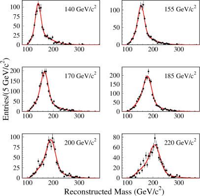
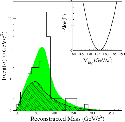
Figure 24: Top quark mass measurement with the template method at CDF in Run I [104]. (a) Top mass distributions of $t\bar{t}$ signal Monte Carlo for six different values of $M_{\mathrm{top}}$ (dots). The overlayed curves are the fitted template functions for that particular top quark mass. (b) The histogram shows the reconstructed top mass distribution for all subsamples combined. The shaded region indicates the fitted signal component, the hatched region the fitted background. The inset shows the log likelihood as a function of the top quark mass.

Using the template functions and the observed mass distribution a likelihood function is defined. The template parameters and the background fraction are constrained to their central values within their uncertainties. The only parameter which is entirely unconstrained is $M_{\mathrm{top}}$. The log likelihood function is minimized with respect to all parameters in a combined fit to all subsamples. The result of the minimization for the combined sample is shown in figure 24b. The minimum of the likelihood is reached for a top quark mass of $M_{\mathrm{top}}=176.1^{+5.2}_{-5.0}\;\mathrm{GeV}/c^{2}$. The given uncertainties are only statistical. Systematic uncertainties due to various sources are evaluated. The biggest uncertainty originates from the jet energy measurement ($4.4\,\mathrm{GeV}/c^{2}$). The modelling of initial and final state radiation causes an uncertainty of $2.6\,\mathrm{GeV}/c^{2}$. The modelling of the shape of the background spectrum induces an uncertainty of $1.3\,\mathrm{GeV}/c^{2}$. Smaller sources of uncertainties are: the $b$ tagging efficiency ($0.4\,\mathrm{GeV}/c^{2}$), parton distribution functions ($0.3\,\mathrm{GeV}/c^{2}$), and Monte Carlo generators ($0.1\,\mathrm{GeV}/c^{2}$). The contributions of all effects are added in quadrature resulting in a total systematic uncertainty of $5.3\,\mathrm{GeV}/c^{2}$.

7.2 Matrix element method

Originally DØ also used a template method to measure the top quark mass. This method used a kinematically fitted mass, similar to CDF, and in addition discriminants based on a likelihood ratio or a neural network [243]. In 2004 DØ reanalyzed its top mass data sample with a new technique based on a matrix element method, which we will describe below [106].

The new measurement is based on the same data set of 91 lepton-plus-jets events as the previous one. The basic selection cuts are very similar to those used for the $t\bar{t}$ cross section measurement [244]. The data set corresponds to an integrated luminosity of $125\;\mathrm{pb^{-1}}$. The result of the template analysis is $M_{\mathrm{top}}=173.3\pm 5.6\;(\mathrm{stat.})\pm 5.5\;(\mathrm{syst.})\;\mathrm{GeV}/c^{2}$.

The matrix element method is designed to extract more kinematic information from the events than the previous template methods, and thus yield an improved precision. The basic idea of the new method is to exploit the fact that the differential cross section for $t\bar{t}$ production depends sensitively on the top quark mass. The differential cross section can thus be used to calculate a probability for a certain top mass hypothesis. While the differential cross section consists of a phase space term and the matrix element for $t\bar{t}$ production, the matrix element is the more significant part, which motivates the name of the method. Matrix element methods have already been used previously to analyse $t\bar{t}$ dilepton events in CDF [245] and DØ [246, 247, 226]. Since leading order matrix elements are used to calculate the event weights, only events with exactly four jets are used. This jet cut minimizes the effect of higher-order corrections and reduces the number of events from 91 to 71.

The production probability $P(x,M_{\mathrm{top}})$ for a $t\bar{t}$ event with a measured set of variables $x$ at a certain top quark mass $M_{\mathrm{top}}$ is given as a convolution of the differential cross section $d\sigma/dy$ with the parton distribution functions $f$ and the transfer function $W(y,x)$ that maps the measured quantities $x$ into the quantities $y$ at parton level:

$$P(x,M_{\mathrm{top}})=\frac{1}{\sigma_{\mathrm{total}}}\;\int\rmd y\,\rmd q_{1}\,\rmd q_{2}\;\frac{\rmd\sigma(y,M_{\mathrm{top}})}{\rmd y}\;f(q_{1})f(q_{2})\;W(y,x)\ .$$ (35)

The parton distribution functions $f(q_{i})$ are evaluated for the incoming partons with momentum fraction $q_{i}$. The integral in (35) is properly normalized by dividing by the total cross section $\sigma_{\mathrm{total}}$. The integration runs over fifteen sharply measured variables, which are directly assigned to the parton quantities without invoking a transfer function. These variables are the eight jet angles, the three-momentum of the lepton, and four equations of energy-momentum conservation. The jet energies are not well measured and a transfer function $W_{\mathrm{jets}}(E_{\mathrm{part}},E_{\mathrm{jet}})$ is needed to map jet energies $E_{\mathrm{jet}}$ measured in the detector to parton level energies $E_{\mathrm{part}}$. The function $W_{\mathrm{jets}}(E_{\mathrm{part}},E_{\mathrm{jet}})$ is a product of four functions $F(E_{\mathrm{part}}^{i},E_{\mathrm{jet}}^{i})$, one for each jet in the event. The functional form of $F$ is the sum of two Gaussians. The parameters of $F$ used for $b$ quarks are different from those for light quark jets. After the first integration step there are five integrals left. One integral runs over the energy of one of the quarks from the hadronic $W$ decay, the other four are over the masses squared, $M_{i}^{2},$ of the two $W$ bosons and the two reconstructed top quarks in the event. This is an economical choice to safe computing time. When computing $P(x,M_{\mathrm{top}})$ all possible 24 permutations of jet assignments and the neutrino $p_{z}$ solution are considered and the average is computed.

Since the candidate sample still contains a considerable amount of background events, it is useful to calculate a background probability $P_{\mathrm{bkg}}(x)$ based on the $W+4$ jets matrix element from Vecbos. Figure 25a shows the $P_{\mathrm{bkg}}$ distribution for the sample of 71 candidate events and an overlay of $t\bar{t}$ and $W+4$ jets Monte Carlo events.

(a)                                                                (b)                               (c)
  

Figure 25: (a) Distribution of the logarithm of the background probability $P_{\mathrm{bkg}}$ for 71 candidate events in the DØ top mass sample [243]. To increase the purity of the sample a cut at $\log(P_{\mathrm{bkg}})<-11$ is performed, as indicated by the vertical line. The data are compared to $t\bar{t}$ signal Monte Carlo (left hatched) and $W+4$ jets background Monte Carlo events (right hatched). (b) Negative of the log likelihood as a function of $M_{\mathrm{top}}$. (c) The likelihood normalized to its maximum value. The curve is fit to a Gaussian. The hatched area corresponds to the 68.27% probability interval.

To reduce the bias in the top mass measurement due to the background content in the sample DØ employs a cut requiring $\log(P_{\mathrm{bkg}})<-11$. After this cut the final top mass sample contains 22 events. The final likelihood for the measurement of $M_{\mathrm{top}}$ is given by

$$-\ln L(M_{\mathrm{top}}) = -\sum_{i=1}^{N}\ln[c_{1}P_{t\bar{t}}(x_{i},M_{\mathrm{top}})+c_{2}P_{\mathrm{bkg}}(x_{i})]+$$ (36)

$$Nc_{1}\int A(x)P_{t\bar{t}}(x,M_{\mathrm{top}})\,\rmd x+Nc_{2}\int A(x)P_{\mathrm{bkg}}(x)\;\rmd x\ .$$

The integrals are calculated using Monte Carlo methods. The acceptance function $A(x)$ is 1.0 or 0.0, depending on whether the event is accepted or rejected by the analysis criteria. The sum runs over all $N=22$ candidate events. The best value of $M_{\mathrm{top}}$ and the parameters $c_{i}$ are defined by minimizing $-\ln L(M_{\mathrm{top}})$, which is shown in figure 25b. Figure 25c shows the likelihood normalized to its maximum value. The Gaussian fit to the likelihood yields a top quark mass of $M_{\mathrm{top}}=(179.6\pm 3.6)\;\mathrm{GeV}/c^{2}$. Monte Carlo studies show that the extracted top quark mass has to be corrected by a shift of $\delta M_{\mathrm{top}}=+0.5\;\mathrm{GeV}/c^{2}$. The total systematic uncertainty of the measurement is 3.9 GeV/$c^{2}$ which is dominated by the uncertainty of the jet energy scale ($3.3\;\mathrm{GeV}/c^{2}$). The final result is $M_{\mathrm{top}}=180.1\pm 3.6\;(\mathrm{stat.})\pm 3.9\;(\mathrm{syst.})\;\mathrm{GeV}/c^{2}$, which is a substantial improvement over the previous template result. The higher precision is mainly due to two differences in the analyses: (a) Well measured events contribute more than poorly measured ones, since a probability is assigned to each event, (b) all possible permutations of the reconstruction are included. Thus, the correct solution always contributes.

7.3 Top quark mass combination

The best precision on the top quark mass is obtained if the individual measurements in the different $t\bar{t}$ channels are combined for each experiment. Further improvement is achieved if the results of the two Tevatron experiments, CDF and DØ, are combined. In the all hadronic channel CDF uses a data sample of 136 events with an estimated background of $108\pm 9$ events [236]. A similar template method as described in section 7.1 gives a result of $186\pm 10\,(\mathrm{stat.})\pm 12\,(\mathrm{syst.})\;\mathrm{GeV}/c^{2}$. Since the dilepton topology comprises two unobserved neutrinos a straightforward full reconstruction of the event is not possible. To get an estimate of $M_{\mathrm{top}}$ on an event-by-event basis a weighting method is used. For each event a weight distribution is calculated as a function of $M_{\mathrm{top}}$. The assigned weight depends on the agreement of the sum of the assumed transverse neutrino momenta with the observed missing transverse energy. The result in the dilepton channel at CDF is $M_{\mathrm{top}}=167.4\pm 10.3\;(\mathrm{stat.})\pm 4.8\;(\mathrm{syst.})\;\mathrm{GeV}/c^{2}$ [248]. The statistical uncertainties of the measurements in the three $t\bar{t}$ channels are uncorrelated, since the samples are statistically independent. However, the systematic uncertainties are correlated. For simplicity, the correlation is either assumed to be 100% or zero. The uncertainties concerning the jet energy scale, the signal model (modelling of ISR and FSR, PDFs and $b$ tagging), and the Monte Carlo generators are set to 100%. The correlation of uncertainties due to Monte Carlo statistics and the background model are assumed to be zero. The combination procedure uses a generalized $\chi^{2}$ method with full covariance matrix and yields a value of $M_{\mathrm{top}}=(176.1\pm 6.6)\;\mathrm{GeV}/c^{2}$ [104].

In the all hadronic channel DØ has measured $M_{\mathrm{top}}=178.5\pm 13.7\;(\mathrm{stat.})\pm 7.7\,(\mathrm{syst.})\;\mathrm{GeV}/c^{2}$ [249]. In the dilepton channel DØ obtains $M_{\mathrm{top}}=168.4\pm 12.3\,(\mathrm{stat.})\pm 3.6\,(\mathrm{syst.})\,\mathrm{GeV}/c^{2}$ [250]. The combination of all $t\bar{t}$ topologies is entirely dominated by the lepton-plus-jets result described in detail in section 7.2 and yields $M_{\mathrm{top}}=(179.0\pm 5.1)\,\mathrm{GeV}/c^{2}$. Combining all CDF and DØ Run I measurements the top quark mass is determined to be

$$M_{\mathrm{top}}=\left(178.0\pm 4.3\right)\;\mathrm{GeV}/c^{2}\ \cite[cite]{[\@@bibref{}{mtopCombined2004}{}{}]}.$$

7.4 Preliminary Run II results

First preliminary Run II measurements of the top quark mass are now available and prepared for publication. CDF has been exploring several different techniques for the measurement of $M_{\mathrm{top}}$. The best single measurement is obtained from an extended mass template technique in the lepton-plus-jets channel. The analysis uses a data sample corresponding to $318\,\mathrm{pb^{-1}}$. The measured invariant mass of the hadronic $W$ boson decay is used to reduce the systematic uncertainty on the jet energy scale. In a two-dimensional likelihood fit the top quark mass and the jet energy scale (JES) are obtained simultaneously. CDF measures $M_{\mathrm{top}}=173.5^{+2.7}_{-2.6}\,(\mathrm{stat.})\pm 2.5\,(\mathrm{JES})\pm 1.7\,(\mathrm{syst.})\,\mathrm{GeV}/c^{2}$.

DØ has presented a preliminary result which is also based on a mass template method. In $b$ tagged lepton-plus-jets events the top quark mass is found to be $M_{\mathrm{top}}=170.6\pm 4.2\,(\mathrm{stat.})\pm 6.0\,(\mathrm{syst.})\,\mathrm{GeV}/c^{2}$. The analysis is based on a data sample of $229\,\mathrm{pb^{-1}}$ and uses 69 candidate events [251].

7.5 Future prospects

The aim of Run II at the Tevatron is to reach a total uncertainty of 2 to 3 GeV/$c^{2}$ on $M_{\mathrm{top}}$. At the LHC the top mass will be measured with negligible statistical uncertainty, while the systematic uncertainty is predicted to be on the order of 1 GeV$/c^{2}$ towards the end of the running period [5]. In this precision regime the concrete definition of the top quark mass becomes relevant. The experiments measure a kinematic top quark mass which is approximately equal to the pole mass that appears in the perturbative top quark propagator. The ambiguity between pole and kinematic mass is on the order of 1 GeV and due to the fact that at this level the top quark cannot be treated as a free quark anymore. At a future linear collider an energy scan in the threshold region for $t\bar{t}$ production will allow a very precise measurement of the $\mathrm{\overline{MS}}$ mass $\overline{M}_{\mathrm{top}}(\mu)$. An uncertainty of 20 MeV is envisaged.

8 Top quark production and decay properties

While the $t\bar{t}$ cross section and top mass measurements have established data samples that are compatible with SM top quark production, it is crucial to check whether the candidate events are in agreement with other predictions made for the SM top quark. In this chapter we discuss the investigation of various production and decay properties of top quarks: the helicity of $W$ bosons from the top quark decay, the measurement of $R_{tb}$, the ratio of branching ratios for $t\rightarrow W+b$ and $t\rightarrow W+q$, the search for the $t\bar{t}$ tau modes, the analysis of spin correlations among the $t\bar{t}$ pair, the measurement of the top quark $p_{\mathrm{T}}$ spectrum, and the search for electroweak top quark production.

8.1 W helicity in top quark decays

As discussed in chapter 3.3 the $V-A$ structure of the electroweak charged current interaction causes the $W$ bosons from the top quark decay to be polarized. The fraction $\mathcal{F}_{0}$ of longitudinal $W$ bosons (helicity $h_{W}=0$) is predicted to be

$$\mathcal{F}_{0}=\frac{M_{\mathrm{top}}^{2}/2M_{W}^{2}}{1+M_{\mathrm{top}}^{2}/2M_{W}^{2}}=(71\pm 1)\%\ ,$$ (37)

where we have used $M_{\mathrm{top}}=(178.0\pm 4.3)\;\mathrm{GeV}/c^{2}$. For $W^{+}$ bosons the remaining 29% are left-handed ($h_{W}=-1$), for $W^{-}$ bosons 29% are right-handed ($h_{W}=+1$). In the SM right-handed $W^{+}$ and left-handed $W^{-}$ are strongly suppressed (branching fraction: 0.04%). In the following discussion we refer only to the $W^{+}$, but imply the $CP$-conjugate statement for the $W^{-}$.

8.1.1 The lepton $p_{\mathrm{T}}$ spectrum

We consider further the leptonic decay of the $W$ boson into $e\nu_{e}$ or $\mu\nu_{\mu}$. The $V-A$ structure of the $W$ boson decay causes a strong correlation between the helicity of the $W$ boson and the lepton momentum. Qualitatively, this can be understood as follows: The $\nu_{\ell}$ from the $W^{+}$ decay is always left-handed, the $\ell^{+}$ is right-handed. In the case of a left-handed $W^{+}$ boson angular momentum conservation demands therefore that the $\ell^{+}$ is emitted in the direction of the $W^{+}$ spin, that means anti-parallel to the $W^{+}$ momentum. That is why, charged leptons from the decay of left-handed $W$ boson are softer than charged leptons from longitudinal $W$ bosons, which are mainly emitted in the direction transverse to the $W$ boson momentum. The spectrum of leptons from right-handed $W$ bosons would be even more harder than the one from longitudinal ones, since they would be emitted preferentially in the direction of the $W$ momentum. Figure 26a shows the $p_{\mathrm{T}}$ distributions of leptons for different $W$ helicities.

(a)                                                                  (b)
   

Figure 26: (a) Transverse momentum distributions of leptons from the $W$ decay for the three different $W$ helicities. The solid dots are from $W^{+}$ bosons with negative helicity or $W^{-}$ bosons with positive helicity. The open circles are from longitudinally polarized $W$ bosons. The closed squares are for leptons from right-handed $W^{+}$ bosons or from left-handed $W^{-}$ bosons. All three distributions are normalized to the same area. The figure is taken from reference [252]. (b) Lepton $p_{\mathrm{T}}$ distributions of the CDF Run I $W$ helicity analysis in the lepton-plus-jets and the dilepton sample [252]. The data (dots with error bars) are compared with the result of the combined fit (solid line) and with the background component (dashed line).

The significant differences for the three helicity states are apparent and exploited by a CDF analysis which uses the dilepton and lepton-plus-jets data samples [252]. The threshold at 20 GeV/$c^{2}$ seen in figure 26a is due to the event selection. Out of the standard dilepton sample the helicity analysis uses only those events that feature leptons of different flavour, one electron and one muon. This additional requirement removes the major part of the Drell-Yan background. Seven dilepton events remain. The lepton-plus-jets sample is divided into three subsamples: (1) events with at least one secondary vertex $b$ tag, (2) events with at least one soft lepton tag, but no secondary vertex tag, and (3) events with no $b$ tags. In the first two subsamples at least three jets with $E_{\mathrm{T}}>15\;\mathrm{GeV}$ and at least one jet with $E_{\mathrm{T}}>8\;\mathrm{GeV}$ are required. In the third subsample at least four jets with $E_{\mathrm{T}}>15\;\mathrm{GeV}$ are mandatory. All jets are counted in the pseudorapidity region $|\eta|<2.4$.

An unbinned maximum likelihood fit to the observed lepton $p_{\mathrm{T}}$ spectrum in each subsample is used to determine the fraction of top quark events that decay to longitudinal $W$ bosons. The likelihood functions for each subsample are added and simultaneously minimized. In the fit function the lepton $p_{\mathrm{T}}$ spectrum for each subsample is parametrized as the product of an exponential and a polynomial. Figure 26b shows the observed lepton $p_{\mathrm{T}}$ spectrum for the dilepton sample and the sum of all three lepton-plus-jets samples. The figure also shows the fit result (signal + background) and the background component alone. The likelihood fit yields a result of $\mathcal{F}_{0}=0.91\pm 0.37\,(\mathrm{stat.})\pm 0.13\,(\mathrm{syst.})$. The largest contribution to the systematic uncertainty is due to the uncertainty in the top quark mass, $\delta\mathcal{F}_{0}=0.07$. The second largest source of uncertainty ($\delta\mathcal{F}_{0}=0.06$) is due to the normalization uncertainty of the non-$W$ background which peaks at low $p_{\mathrm{T}}$ and thereby mimics the shape of the lepton $p_{\mathrm{T}}$ distribution coming from negative helicity $W$ bosons. Other sources of systematic uncertainties are the $b$ tagging efficiency, Monte Carlo statistics, the modelling of gluon radiation, and uncertainties in the parton distribution functions.

CDF has applied the same method as described above to measure $\mathcal{F}_{0}$ in Run II data. The new analysis is based on data samples corresponding to $162\,\mathrm{pb}^{-1}$ or $193\,\mathrm{pb}^{-1}$ for the lepton-plus-jets or the dilepton sample, respectively. The result for the combined sample is $\mathcal{F}_{0}=0.31^{+0.37}_{-0.23}\,(\mathrm{stat.})\pm 0.17\,(\mathrm{syst.})$ [253].

8.1.2 Measurement of $\mathcal{F}_{0}$ with the matrix element method

DØ has used the matrix element method that is employed for the top quark mass measurement, see section 7.2, to determine the longitudinal polarization fraction $\mathcal{F}_{0}$ [254]. The data sample consists of the same 22 events that are analyzed for the mass measurement. The $t\bar{t}$ probability density $P_{\mathrm{t\bar{t}}}(x,\mathcal{F}_{0})$ includes contributions with longitudinal helicity ($\mathcal{F}_{0}$) and negative helicity ($\mathcal{F}_{-}$), but only the ratio $\mathcal{F}_{0}/\mathcal{F}_{-}$ is allowed to vary. The likelihood maximization yields $\mathcal{F}_{0}=0.56\pm 0.31\,(\mathrm{stat.})\pm 0.07\,(\mathrm{syst.})$. The statistical error also contains a contribution from the top quark mass uncertainty which is included in the measurement by integrating over the mass from $M_{\mathrm{top}}=165\;\mathrm{GeV}/c^{2}$ to $M_{\mathrm{top}}=190\;\mathrm{GeV}/c^{2}$. The result for $\mathcal{F}_{0}$ is in good agreement with the SM prediction.

8.1.3 The helicity angle $\cos\theta_{\ell W}$

Another possibility to measure the polarization of $W$ bosons from top quark decays is to reconstruct the helicity angle $\theta_{\ell W}$, which is defined as the angle between the lepton momentum in the $W$ rest frame and the $W$ momentum in the top quark rest frame. Leptons from the decay of longitudinally polarized $W$ bosons have a symmetric angular distribution of the form $1-\cos^{2}\theta_{\ell W}$. Leptons from left-handed $W$ bosons have an asymmetric angular distribution of the form $(1-\cos\theta_{\ell W})^{2}$, while right-handed $W$ bosons would have a distribution of the form $(1+\cos\theta_{\ell W})^{2}$.

The direct reconstruction of $\cos\theta_{\ell W}$ requires information on the top quark and $W$ rest frames and thus, the reconstruction of the respective momenta. Experimentally, the determination of $\bi{p}_{\mathrm{top}}$ and $\bi{p}_{W}$ is difficult, since it relies on the relatively poor measurement of jets and the $\bi{E}_{\mathrm{T}}\!\!\!\!\!\!\!/\;\;$. However, there is a very good approximation which relates $\cos\theta_{\ell W}$ to the invariant mass of the lepton and the $b$ quark jet from the top quark decay:

$$M_{\ell b}^{2}=\frac{1}{2}(M_{\mathrm{top}}^{2}-M_{W}^{2})\;(1+\cos\theta_{\ell W})\ .$$ (38)

Using the quantity $M_{\ell b}^{2}$ instead of $\cos\theta_{\ell W}$ circumvents the difficulties related to direct top quark reconstruction.

CDF has exploited relation (38) to search for an anomalously large right-handed fraction $\mathcal{F}_{+}$ of $W$ bosons in Run I data [255]. The large top quark mass has led to speculations that the top quark could play an active role in electroweak symmetry breaking, which would lead to anomalous electroweak interactions of the top quark [2]. One possibility are left-right symmetric models that lead to a significant right-handed fraction of $W$ bosons in top quark decays. An additional $V+A$ component would lead to a lower left-handed fraction, but leave the longitudinal fraction $\mathcal{F}_{0}$ unchanged. For the analysis CDF uses the same 7 dilepton events as for the lepton $p_{\mathrm{T}}$ analysis mentioned earlier in section 8.1.1. Since the tagging of $b$ quark jets is not employed in the dilepton sample, there are four $M_{\ell b}^{2}$ combinations for each dilepton event. In the lepton-plus-jets sample at least one $b$ tagged jet is required. There are 15 events with exactly one $b$ tag and 5 events with two tags. The $M_{\ell b}^{2}$ distributions are fit to a linear combination of template distributions for the three $W$ polarization states. Only the shape information is used, the normalization is left floating. The fit maximizes a binned likelihood as a function of $f_{V+A}$, the right-handed fraction of the $Wtb$ vertex. If there are two possible $b$ jets that can be matched to the primary lepton, the fit is performed to two-dimensional distributions taking both solutions into account. The fit result is $f_{V+A}=-0.21^{+0.42}_{-0.24}\;(\mathrm{stat.})\pm 0.21(\mathrm{syst.})$ which is an unphysical value, but gives more preference to the SM $V-A$ interaction rather than a $V+A$ contribution. The dominating systematic uncertainty is due to the uncertainty in the top quark mass, which contributes $0.19$ to the total systematic uncertainty of $0.21$. The result can be converted into a one-sided upper limit of $f_{V+A}<0.80$ at the 95% confidence level (C.L.). If one assumes the longitudinal fraction to have the SM value this limit corresponds to $\mathcal{F}_{+}<0.24$ at the 95% C.L.. This result can be combined with the measurement obtained from the lepton $p_{\mathrm{T}}$ analysis. The correlation of the two results is about 40%. The combination yields an improved limit of $\mathcal{F}_{+}<0.18$ at the 95% C.L., which is inconsistent with a pure $V+A$ theory at a confidence level equivalent to the probability of a $2.7\;\sigma$ Gaussian statistical fluctuation.

In Run II CDF has provided a preliminary measurement of $\mathcal{F}_{0}$ using the $M_{\ell b}^{2}$ method. The analyzed data sample consists of 31 lepton-plus-jets events with one secondary vertex $b$ tag. The resulting value is $\mathcal{F}_{0}=0.99^{+0.29}_{-0.35}\,(\mathrm{stat.})\pm 0.19\,(\mathrm{syst.})$ [253].

8.2 Measurement of $R_{tb}$

In the SM the top quark is predicted to decay to a $W$ boson and a $b$ quark with a branching fraction of nearly 100%. This is a consequence of the CKM matrix element $|V_{tb}|$ being close to unity. Our knowledge on $|V_{tb}|$ comes primarily from measurements of $b$ meson decays using the unitarity condition of the CKM matrix ($\mathbf{VV^{\dagger}}=\mathbf{V^{\dagger}V}=\mathbf{1}$). This indirect method yields $0.9990<|V_{tb}|<0.9992$ with high precision [10]. However, if a fourth generation of quarks was present, unitarity of the CKM matrix could be violated. Therefore, it is desirable to make a direct measurement of the top quark branching fraction to $Wb$.

In Tevatron Run I CDF has measured the ratio $R_{tb}=\mathrm{BF}(t\rightarrow Wb)/\mathrm{BF}(t\rightarrow Wq)$, where $q$ can be any down-type quark [256]. The analysis uses 9 events from the dilepton sample and 163 events from the lepton-plus-jets sample. The ratio $R_{tb}$ is measured from the data by comparing the observed number of events with secondary vertex $b$ tags or soft lepton $b$ tags to the number of expected events based on the kinematic acceptances, tagging efficiencies and background estimates. Four event categories are considered: (1) events with no $b$ tags, (2) events with one or more soft lepton tags, (3) events with exactly one secondary vertex tag, and (4) events with two secondary vertex tags. In the dilepton sample only secondary vertex $b$ tagging is used. A maximum likelihood fit yields $R_{tb}=0.94^{+0.26}_{-0.21}\,(\mathrm{stat.})\,^{+0.17}_{-0.12}\,(\mathrm{syst.})$, consistent with the SM prediction. The result can also be expressed as a lower limit: $R_{tb}>0.56$ at the 95% C.L..

The CKM matrix element $|V_{tb}|$ is related to $R_{tb}$, although in a model-dependent way. Under the assumption that the top quark decays only to $Wq$ final states and using three generation unitarity one finds $R_{tb}=|V_{tb}|^{2}$. As a result, CDF finds $|V_{tb}|=0.97^{+0.16}_{-0.12}$ or $|V_{tb}|>0.75$ at the 95% C.L. [256].

In Run II CDF has obtained a preliminary result of this analysis using only the secondary vertex $b$ tag algorithm and improved the lower limit to $R_{tb}>0.61$ at the 95% C.L. [257]. DØ has performed a similar analysis in the lepton-plus-jets sample using the secondary vertex and the impact parameter $b$ tag method. The preliminary results are $R_{tb}=0.70^{+0.27}_{-0.24}\,(\mathrm{stat.})\,^{+0.11}_{-0.10}\,(\mathrm{syst.})$ for the secondary vertex tagged sample and $R_{tb}=0.65^{+0.34}_{-0.30}\,(\mathrm{stat.})\,^{+0.17}_{-0.12}\,(\mathrm{syst.})$ for events with an impact parameter tag [258].

8.3 Search for $\mu\tau$ and $e\tau$ top decays in $t\bar{t}$ events

Up to now the searches for the $t\bar{t}$ tau decay modes have not produced enough evidence to claim the observation of this channel. We discuss in this paragraph the latest search by CDF using Run II data corresponding to an integrated luminosity of $194\,\mathrm{pb^{-1}}$ [259]. The search is carried out in the $t\bar{t}$ tau dilepton channel where one $W$ boson decays into $e\nu_{e}$ or $\mu\nu_{\mu}$ and the second $W$ boson decays into $\tau\nu_{\tau}$ with a subsequent hadronic decay of the tau lepton. The branching fraction of this $t\bar{t}$ mode is about 5%, the same size as the classical dilepton channel ($ee$, $e\mu$, $\mu\mu$). However, several factors lead to a reduced acceptance for the tau mode: the hadronic branching ratio of the tau is 64%, the kinematic acceptance is reduced due to the undetected neutrino, and the tau selection is less efficient than the electron or muon selection. In total, the event detection efficiency for the tau modes is about five times smaller than the one for the standard dilepton analysis. This fact mainly explains why the tau mode so far evaded observation.

The data set for the CDF analysis was selected by a trigger on high-$p_{\mathrm{T}}$ electrons and muons. It is the same data set used for the dilepton cross section measurement discussed in section 6.1. On analysis level electrons and muons are identified using standard cuts as mentioned in the description of the dilepton analysis. Hadronic tau decays have a distinct signature of narrow isolated jets with low charged track multiplicity. A tau candidate is defined by two components: (1) A calorimeter cluster containing a seed tower with $E_{\mathrm{T}}>6\,\mathrm{GeV}$ and a maximum of five adjacent towers with $E_{\mathrm{T}}>1\,\mathrm{GeV}$. (2) At least one track with $p_{\mathrm{T}}>4.5\,\mathrm{GeV}/c$ is required to point to the tau calorimeter cluster. Further cuts are employed to reduce background. A cone is defined around the seed track using a variable radius of $\theta_{\mathrm{cone}}=\mathrm{min}\{0.17,\;(5\,\mathrm{GeV})/E_{\mathrm{cluster}}\}\,\mathrm{rad}$. Within this cone there must be exactly one or three tracks with $p_{\mathrm{T}}>1\,\mathrm{GeV}/c$ including the seed track. In the case of three tracks, the charges must not all be positive or negative. Within an isolation annulus extending from the outer edge of the tau cone to $30^{\circ}$ no tracks or $\pi^{0}$ candidates are allowed. The $\pi^{0}$ candidates are identified in the calorimeter by clusters of energy in the shower maximum detector. The transverse momentum of the tau is estimated by the sum of the track $p_{\mathrm{T}}$ plus the $E_{\mathrm{T}}/c$ of $\pi^{0}$ candidates identified within the tau cone. Additional requirements on the tau candidate are $p_{\mathrm{T}}>15\,\mathrm{GeV}/c$ and $m_{\mathrm{candidate}}<1.8\,\mathrm{GeV}/c^{2}$. The calorimeter towers within the isolation annulus are required to have $E_{\mathrm{T}}$ less than 6% of the tau candidate $E_{\mathrm{T}}$. Electrons or muons that fake tau candidates are removed by asking that the energy in the hadron calorimeter divided by the sum of the tau track momenta is above 0.15, and that the $E_{\mathrm{T}}$ of the tau calorimeter cluster divided by the tau seed track is above 0.5. Additional requirements on candidate events are: $E_{\mathrm{T}}\!\!\!\!\!\!\!/\ \;>20\,\mathrm{GeV}$, and at least two jets within $|\eta|<2.0$. The first jet has to have $E_{\mathrm{T}}>25\,\mathrm{GeV}$, the second jet $E_{\mathrm{T}}>15\,\mathrm{GeV}$. The scalar sum of the electron or muon $p_{\mathrm{T}}$, the tau $p_{\mathrm{T}}$, the $E_{\mathrm{T}}\!\!\!\!\!\!\!/\ \;$, and the $E_{\mathrm{T}}$ of the jets is defined as $H_{\mathrm{T}}$ and must exceed 205 GeV. Including all branching ratios, kinematic cuts and efficiencies the event detection efficiency for $t\bar{t}$ events is found to be $\epsilon_{\mathrm{evt}}=(0.080\pm 0.015)\%$.

The number of expected $t\bar{t}$ events is $1.00\pm 0.17$. The estimated background is $1.29\pm 0.25$ events. The dominant contributions to the background are $W+\mathrm{jets}$ events where a jet fakes a tau (58%), $Z^{0}\rightarrow\tau^{+}\tau^{-}+\mathrm{jets}$ (19%), $WW$ production (11%), and $Z^{0}\rightarrow e^{+}e^{-}+\mathrm{jets}$ where an electron fakes a tau (6%). In CDF II data two events are observed, compatible with the SM expectation. The significance of the result is not high enough to claim the observation of the $t\bar{t}$ tau mode. The result can be converted into an upper limit on an anomalous enhancement of the $t\rightarrow\tau\nu_{\tau}q$ rate. An enhancement of more than a factor of 5.2 is excluded at the 95% confidence level. The Run II analysis has improved the expected signal to background ratio over the previous Run I $t\bar{t}$ tau analysis of CDF [260] from 0.5 to 0.78. With more data to come in Run II this improvement brings the observation of the $t\bar{t}$ tau mode within reach. In the Run I analysis 4 candidate events are observed over a background of 2 events and a signal expectation of 1 event.

8.4 Spin correlations in $t\overline{t}$ events

As discussed in detail in section 3.3, top quarks decay as quasi-free quarks due to their short lifetime. Thus, the spin information of top quarks is transmitted to the decay products and is accessible experimentally. In this way top quarks are a unique laboratory to study spin aspects of heavy quark production, contrary to $b$ quarks where the hadronization to $b$ hadrons removes the initial spin information. At the Tevatron $t\bar{t}$ pairs are produced unpolarized. However, the spins of the top and antitop quark are expected to have a strong correlation and point along the same axis in the $t\bar{t}$ rest frame on an event-by-event basis.

An optimal spin quantization axis can be constructed using the velocity $\beta^{*}$ and the scattering angle $\theta^{*}$ of the top quark with respect to the centre-of-mass frame of the incoming partons. The quantization axis forms the angle $\psi$ with respect to the $p\bar{p}$ beam axis [261]:

$$\tan\psi=\frac{\beta^{*2}\sin\theta^{*}\cos\theta^{*}}{1-\beta^{*2}\sin^{2}\theta^{*}}\ .$$ (39)

For the $q\bar{q}\rightarrow t\bar{t}$ process the spins of the top and the antitop quark are fully aligned along the same direction in this spin basis. If the gluon fusion process $gg\rightarrow t\bar{t}$ is included the correlation is reduced. In the limit where the $t\bar{t}$ pair is produced at rest ($\beta^{*}=0$) the spins are pointing along the beam axis. The spin correlation of the $t\bar{t}$ pair is transmitted to the top quark decay products. Experimentally, it is particularly advantageous to investigate correlations of the primary leptons in $t\bar{t}$ dilepton events. The observables are the angles $\theta_{-}$ and $\theta_{+}$ between the momenta of the negatively or positively charged leptons in the rest frame of their parent top quark and the spin quantization axis. Using these angles the spin correlation can be expressed by the differential cross section [262]

$$\frac{1}{\sigma_{\mathrm{total}}}\cdot\frac{\rmd^{2}\sigma}{\rmd(\cos\theta_{+})\rmd(\cos\theta_{-})}=\frac{1+\kappa\cos\theta_{+}\,\cos\theta_{-}}{4}\ ,$$ (40)

where $\kappa$ is the correlation coefficient which is predicted to be $\kappa=0.88$ at the Tevatron (Run I). The coefficient $\kappa$ can vary between $-1$, fully negative correlation, and $\kappa=+1$ for a fully positive correlation.

The DØ collaboration has searched for evidence of $t\bar{t}$ spin correlations in Run I data using dilepton events [263]. Since the angles $\theta_{-}$ and $\theta_{+}$ are measured in the top quark rest frame, the top quark has to be fully reconstructed. In dilepton events this cannot be achieved unambiguously, since the two neutrinos are not reconstructed. Up to four different solutions per event have to be considered. A weight is assigned to each solution based on how well the sum of the transverse momenta of the two neutrinos in the solution agrees with the measured $E_{\mathrm{T}}\!\!\!\!\!\!\!/\ \;$. For each solution the leptons are boosted into the respective top quark rest frame and $\cos\theta_{+}$ or $\cos\theta_{-}$ are computed.

To deduce $\kappa$ the two-dimensional phase space of $(\cos\theta_{+},\,\cos\theta_{-})$ is used in a binned likelihood analysis. The bins are filled with the event weights obtained from the event fitter. Since an event populates each bin with fractional probability, the likelihood fit does not use a simple Poisson likelihood. The correlation between different bins is obtained from Monte Carlo events and the bin contents of the $(\cos\theta_{+},\,\cos\theta_{-})$ space are rotated such, that they are uncorrelated. The new variables are used to construct the likelihood. DØ uses six dilepton data events, three $e\mu$, two $ee$ and one $\mu\mu$ event. The fit result from data is used to compute a lower limit of $\kappa>-0.25$ at the 68% confidence level, which is in agreement with the SM expectation of $\kappa=0.88$.

8.5 The top quark $p_{\mathrm{T}}$ spectrum

The CDF collaboration has further investigated the kinematics of $t\bar{t}$ events by measuring the top quark $p_{\mathrm{T}}$ spectrum [264]. This analysis is partially motivated by exotic models that predict alternative production mechanisms for top quarks at the Tevatron, in particular an enhancement of top quarks with transverse momentum above 200 GeV/$c$. The Run I lepton-plus-jets data set with secondary vertex $b$ tag or soft lepton tag are used in the analysis. The events are subjected to a kinematic fit similar to the top quark mass analysis described in section 7.1. The invariant mass reconstructed from the top quark decay products is constrained to $175\,\mathrm{GeV}/c^{2}$. Events with $\chi^{2}>10$ from the fit are rejected. The final data sample contains 61 candidate events. Figure 27a shows the $p_{\mathrm{T}}$ distribution of the hadronically decaying top quark.

(a)                                                                 (b)
   

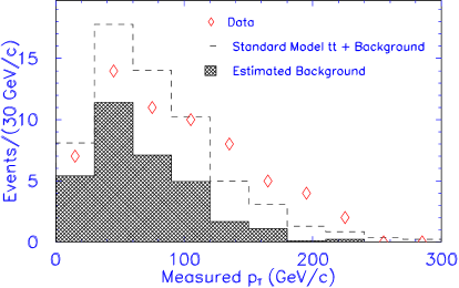
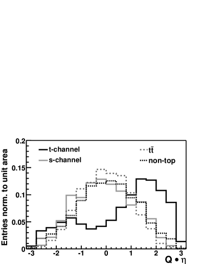
Figure 27: (a) Transverse momentum distribution of hadronically decaying top quarks from 61 candidate events of reference [264]. The hatched distribution shows the estimated background, the dashed distribution the SM prediction of background plus $t\bar{t}$ production. (b) $Q\cdot\eta$ distributions for Monte Carlo templates normalized to unit area. The $Q\cdot\eta$ distribution is used in the CDF Run II single top analysis to distinguish between $t$-channel and $s$-channel single top events [265].

The differences in the spectrum do not constitute a significant deviation from the SM prediction. A maximum likelihood technique is used to estimate the fraction $R_{4}$ of top quarks in the high transverse momentum region of $225<p_{\mathrm{T}}<425\,\mathrm{GeV}/c$. The measured fraction is $R_{4}=0.0^{+0.04}_{-0.0}$, while the SM expectation is $R_{4}=0.025$. The data result can be converted into an upper limit of $R_{4}<0.16$ at the 95% confidence level.

8.6 Electroweak top quark production

While $t\bar{t}$ pair production via the strong interaction is the dominant source of top quarks at the Tevatron (and also at the LHC), top quarks can also be produced as single quarks via the electroweak interaction. The theoretical aspects of single top production are discussed in section 3.2 of this review. The relevant modes are $t$-channel and $s$-channel production, see figure 10. Several analyses have searched for electroweak top quark production in Tevatron Run I data [266, 267, 268, 269]. The best upper limits obtained on the production cross sections in Run I are $13\,\mathrm{pb}$ at the 95% C.L. for the $t$-channel [268] and $17\,\mathrm{pb}$ at the 95% C.L. for the $s$-channel [267].

The CDF collaboration has published the first search for single top production in Run II [265]. In the following paragraphs we will briefly review this analysis which uses a data sample corresponding to an integrated luminosity of $(162\pm 10)\,\mathrm{pb^{-1}}$. The event selection is essentially the same as the one used for the $t\bar{t}$ cross section measurement in lepton-plus-jets events with secondary vertex $b$ tagging, see section 6.2.2. The jet definition differs in the pseudorapidity range. While the $t\bar{t}$ cross section measurement counts jets up to $|\eta|<2.0$, the range is enlarged in the single top analysis to $|\eta|<2.8$. This change is motivated by an increase in acceptance for the $t$-channel process in the $W+2\,\mathrm{jets}$ sample by roughly 30%. Exactly two jets are required. At least one of these jets must be identified as a $b$ quark jet by a secondary vertex tag. To optimize the sensitivity, CDF applies a cut on the invariant mass $M_{\ell\nu b}$ of the charged lepton, the neutrino and the $b$ tagged jet: $140\;\mathrm{GeV}/c^{2}\leq M_{\ell\nu b}\leq 210\;\mathrm{GeV}/c^{2}$. The transverse momentum of the neutrino is set equal to the missing transverse energy vector $\bi{E}_{\mathrm{T}}\!\!\!\!\!\!\!/\;\;$; $p_{z}(\nu)$ is obtained up to a two-fold ambiguity from the constraint $M_{\ell\nu}=M_{W}$. From the two solutions the one with the lower $|p_{z}(\nu)|$ is chosen. If the $p_{z}(\nu)$ solution has non-zero imaginary part as a consequence of resolution effects in measuring jet energies, only the real part of $p_{z}(\nu)$ is used. Two analyses are performed on this data sample: (1) a separate search, which measures the rates for the two single top processes, $t$-channel and $s$-channel, individually, and (2) a combined search where $t$- plus $s$-channel are treated as one single top signal. For the separate search, the data sample is subdivided into events with exactly one $b$ tagged jet or exactly two $b$ tagged jets. For the 1-tag sample, at least one jet is required to have $E_{\mathrm{T}}\geq 30\;\mathrm{GeV}$.

The event detection efficiency for the signal is determined from events generated by the matrix element event generator MadEvent [270, 271], followed by parton showering with Pythia [171] and a full CDF II detector simulation. MadEvent features the correct spin polarization of the top quark and its decay products. For $t$-channel single top production two samples are generated, one $b+q\rightarrow t+q^{\prime}$ and one $g+q\rightarrow t+\bar{b}+q^{\prime}$ which are merged together to reproduce the $p_{\mathrm{T}}$ spectrum of the $\bar{b}$ as expected from NLO differential cross section calculations. This is an improved model compared to the Pythia modelling used in the Run I analyses. The event detection efficiency $\epsilon_{\mathrm{evt}}$ includes the kinematic and fiducial acceptance, branching ratios, lepton and $b$ jet identification as well as trigger efficiencies. In the 1-tag sample one finds $\epsilon_{\mathrm{evt}}=(0.86\pm 0.07)\%$ for the $t$-channel and $\epsilon_{\mathrm{evt}}=(0.78\pm 0.06)\%$ for the $s$-channel.

Two background components are distinguished: $t\bar{t}$ and nontop background. The nontop background is estimated using the same method as used for the $t\bar{t}$ cross section analysis, see section 6.2.2. The primary source (62%) of the nontop background is the $W$+heavy flavour processes $\bar{q}q^{\prime}\rightarrow Wg$ with $g\rightarrow b\bar{b}$ or $g\rightarrow c\bar{c}$, and $gq\rightarrow Wc$. Additional sources are “mistags” (25%), in which a light quark jet is erroneously identified as heavy flavour, “non-$W$”(10%), e.g. direct $b\bar{b}$ production, and diboson ($WW$, $WZ$, $ZZ$) production (3%). The non-$W$ and mistag fractions are estimated using CDF II data. The $W$+heavy flavour rates are extracted from Alpgen [178] Monte Carlo events normalized to data. The diboson rates are estimated from Pythia events normalized to theory predictions [272]. After all selection cuts CDF observes 33 events in the 1-tag sample, 6 events in the 2-tag sample, and 42 events for the combined search. Within the uncertainties, the observations are in good agreement with predictions.

To extract the signal content in data, a maximum likelihood technique is employed. Separation of $t$- and $s$-channel events is achieved by using the $Q\cdot\eta$ distribution which exhibits a distinct asymmetry for $t$-channel events, see figure 27b. $Q$ is the charge of the primary lepton and $\eta$ is the pseudorapidity of the untagged jet. Figure 28a shows CDF data versus stacked Monte Carlo templates weighted by the expected number of events in the 1-tag sample.

(a)                                                                  (b)
   

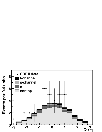
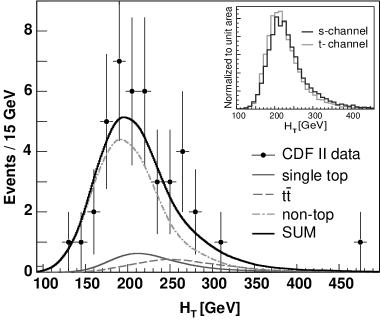
Figure 28: Search for electroweak top quark production at CDF in Run II [265]. (a) $Q\cdot\eta$ distribution for CDF data in the 1-tag sample (33 events) versus stacked Monte Carlo templates normalized to the SM prediction. (b) $H_{\mathrm{T}}$ distribution for data (42 events) in the combined single top search, compared with smoothed Monte Carlo predictions for signal and background. The inset shows the $H_{\mathrm{T}}$ distributions for $t$-channel and $s$-channel single top production to demonstrate that these distributions are very similar and may be combined.

The separate search defines a joint likelihood function for the $Q\cdot\eta$ distribution in the 1-tag sample and for the number of events in the 2-tag sample. The background rates are constrained to their SM prediction by Gaussian priors. The systematic uncertainties are taken into account in the likelihood definition. Systematic shifts in the acceptance and in the shape of the $Q\cdot\eta$ template histograms, and their full correlation are considered. The largest uncertainties on the acceptance are due to the uncertainty on the $b$ tagging efficiency (7%), the luminosity (6%), the top quark mass (4%), and the jet energy scale (4%). The likelihood procedure yields a most probable value of $0.0^{+4.7}_{-0.0}\,\mathrm{pb}$ for the $t$-channel cross section, and $(4.6\pm 3.8)\,\mathrm{pb}$ for the $s$-channel cross section. These results are translated into upper limits on the cross sections which exclude an anomalous enhancement of single top quark production. The upper limit for the $t$-channel is found to be 10.1 pb at the 95% C.L., the upper limit for the $s$-channel is 13.6 pb at the 95% C.L..

To measure the combined $t$-channel plus $s$-channel signal in data, a kinematic variable is used whose distribution is very similar for the two single top processes (see inset of figure 28b), but is different for background processes: $H_{\mathrm{T}}$, which is the scalar sum of $E_{\mathrm{T}}\!\!\!\!\!\!\!/\ \;\;$ and the transverse energies of the lepton and all jets in the event. In figure 28b the $H_{\mathrm{T}}$ distribution observed in data is compared with the SM prediction. A likelihood function similar to that of the separate search yields a most probable value of $7.7^{+5.1}_{-4.9}\,\mathrm{pb}$ for the single top cross section. The resulting upper limit is 17.8 pb at the 95% C.L.. The quoted result (combined search) excludes an anomalous enhancement of single top production which is more than 6.1 times larger than the SM production. However, separate measurements of the $t$-channel and $s$-channel are important because the two processes are sensitive to different new physics contributions, see for example references [273, 274, 275, 276, 277, 278].

DØ has presented results on a single top search using neural networks [279]. With a data sample corresponding to an integrated luminosity of $230\,\mathrm{pb^{-1}}$ DØ can set an upper limit of 5.0 pb at the 95% C.L. on the $t$-channel cross section and 6.4 pb at the 95% C.L. on the $s$-channel cross section. With more data at the Tevatron to come, a first observation of electroweak top quark production is in reach within the next years. Preliminary studies indicate that data corresponding to about $1.5\,\mathrm{fb^{-1}}$ will allow to establish evidence for electroweak top quark production at a probability level excluding a background fluctuation that is equivalent to a $3\,\sigma$ deviation in a Gaussian distribution. Once electroweak top quark production is observed the measurement of the production cross section will allow to directly extract the CKM matrix element $|V_{tb}|$.

9 Search for anomalous couplings

Mainly because of its large mass the top quark has fostered speculations that it offers a unique window to search for physics beyond the SM. One possibility to test this hypothesis is to measure top quark properties and check whether the observation is in agreement with the SM prediction. This approach is based on the measurements that are discussed in previous chapters, involving properties such as the $t\bar{t}$ cross section, the top mass, or the $W$ helicity in top quark decays. A second approach is to search directly for new particles coupling to the top quark or for non-SM decays. In this section we present those topics which have led to specific analyses at the Tevatron. In section 9.4 we will additionally discuss searches for anomalous single top quark production at HERA and LEP.

9.1 Decays to a charged Higgs boson

In the SM a single complex Higgs doublet scalar field is responsible for breaking the electroweak symmetry and generating the masses of gauge bosons and fermions. Many extensions of the SM include a Higgs sector with two Higgs doublets and are therefore called Two Higgs Doublet Models (THDM). In a THDM electroweak symmetry breaking leads to five physical Higgs bosons: two neutral $CP$-even scalars $h^{0}$ and $H^{0}$, one neutral $CP$-odd pseudoscalar $A^{0}$, and a pair of charged scalars $H^{\pm}$. The extended Higgs sector is described by two parameters: the mass of the charged Higgs, $M_{H^{+}}$, and $\tan\beta=v_{1}/v_{2}$, the ratio of the vacuum expectation values $v_{1}$ and $v_{2}$ of the two Higgs doublets. One distinguishes two types of THDMs. In a type I THDM only one of the Higgs doublets couples to fermions, in a type II THDM the first Higgs doublet couples to the up-type quarks ($u$, $c$, $t$) and neutrinos, while the second doublet couples to down-type quarks ($d$, $s$, $b$) and charged leptons. The analyses we discuss in this section are concerned with type II models. A particular example for a type II THDM is the minimal supersymmetric model (MSSM).

If the charged Higgs boson is lighter than the difference of top quark and $b$ quark mass, $M_{H^{\pm}}<M_{\mathrm{top}}-M_{b}$, the decay mode $t\rightarrow H^{+}b$ is possible and competes with the SM decay $t\rightarrow W^{+}b$. The branching fraction depends on $\tan\beta$ and $M_{H^{+}}$. The MSSM predicts that the channel $t\rightarrow H^{+}b$ dominates the top quark decay for $\tan\beta\lesssim 1$ and $\tan\beta\gtrsim 70$. In most analyses it is assumed that $\mathrm{BF}(t\rightarrow W^{+}b)+\mathrm{BF}(t\rightarrow H^{+}b)=1$. At tree level the $H^{\pm}$ does not couple to vector bosons. Therefore, the $H^{\pm}$ decays only to fermions. In the parameter region $\tan\beta<1$ the dominant decay mode is $H^{+}\rightarrow c\bar{s}$, while for $\tan\beta>1$ the decay channel $H^{+}\rightarrow\tau^{+}\nu_{\tau}$ is the most important one. For $\tan\beta>5$ the branching fraction to $\tau^{+}\nu_{\tau}$ is nearly 100%. Thus, in this region of parameter space type II THDM models predict an excess of $t\bar{t}$ events with tau leptons over the SM expectation.

First searches for the $H^{\pm}$ in top quark events were already performed well before the top quark was discovered in 1994/95. The UA1 and UA2 experiments at the CERN $Sp\bar{p}S$ excluded certain regions of the $M_{\mathrm{top}}$ versus $M_{H^{\pm}}$ plane [280, 281]. First searches of CDF improved these limits using events with a dilepton signature [282] or reconstructing tau leptons in their hadronic decay mode [283].

At LEP the experiments searched for charged Higgs production in the process $e^{+}e^{-}\rightarrow H^{+}H^{-}$. The analyses encompass the final states $c\bar{s}\bar{c}s$, $\tau^{+}\nu_{\tau}\tau^{-}\bar{\nu_{\tau}}$, $c\bar{s}\tau^{-}\bar{\nu_{\tau}}$, and $\tau^{+}\nu_{\tau}\bar{c}s$. The combined result of all four experiments excludes charged Higgs masses below $78.6\,\mathrm{GeV}/c^{2}$ [284]. The CLEO collaboration has used its measurement of the inclusive $b\rightarrow s\gamma$ cross section to set an indirect limit on the charged Higgs mass [285]. The dependence of the cross section on $M_{H^{\pm}}$ enters via quantum corrections. Since the process $b\rightarrow s\gamma$ occurs only at loop level in the SM, its sensitivity to new particles which might be exchanged in the loop is quite high. CLEO sets a limit of $M_{H^{\pm}}>(244+63/(\tan\beta)^{1.3})\,\mathrm{GeV}/c^{2}$ at the 95% C.L., under the assumption that a type II THDM is realized in nature. If the Higgs sector has a richer structure, the CLEO limit can be circumvented. Therefore, direct searches for the $H^{\pm}$ which are less model dependent remain important.

After the top quark discovery the $H^{\pm}$ searches at the Tevatron looked for the decay modes $t\bar{t}\rightarrow H^{\pm}W^{\mp}b\bar{b}$ and $t\bar{t}\rightarrow H^{\pm}H^{\mp}b\bar{b}$. CDF published three analyses where the charged Higgs is assumed to decay into $\tau^{+}\nu_{\tau}$ and the tau lepton subsequently decays semi-hadronically into a tau neutrino plus hadrons [286, 287, 288]. The identification of hadronic tau decays in these CDF analyses is similar to the one described in detail in section 8.3. Two analyses (references [286, 287]) used an inclusive approach, based on final states with missing transverse energy, one identified hadronic tau decay, jets or high-$p_{\mathrm{T}}$ leptons. One analysis (reference [288]) requires one high-$p_{\mathrm{T}}$ lepton ($e$ or $\mu$) in the event, which can originate from the decay $W\rightarrow e/\mu+\nu$ or $H^{+}\rightarrow\tau^{+}\nu_{\tau}\rightarrow\bar{\nu}_{\tau}+e^{+}/\mu^{+}+\nu_{e/\mu}+\nu_{\tau}$. The best exclusion limit is obtained from the inclusive analysis [287]: For $M_{H^{\pm}}=80\,\mathrm{GeV}/c^{2}$ the region of $\tan\beta\gtrsim 25$ is excluded. For higher Higgs masses the exclusion becomes less stringent, reaching $\tan\beta\gtrsim 200$ at $M_{H^{\pm}}=160\,\mathrm{GeV}/c^{2}$.

The first DØ search for the $H^{\pm}$ is based on a disappearance strategy, looking for a deficit of events in the SM lepton-plus-jets channel [289]. Since good agreement between the SM prediction and the observation is found, certain regions of phase space for charged Higgs production can be excluded. This result is superseded by a direct search for hadronic tau decays in top quark events [290]. In the following paragraph we will discuss this last Run I analysis on the charged Higgs in more detail.

The DØ analysis uses data taken with a multijet + $E_{\mathrm{T}}\!\!\!\!\!\!\!/\ \;$ trigger corresponding to $(62.3\pm 3.1)\,\mathrm{pb^{-1}}$ of integrated luminosity. Relatively loose preselection cuts are applied, followed by tighter cuts involving an artificial neural network. The preselection requires that $E_{\mathrm{T}}\!\!\!\!\!\!\!/\ \;>25\,\mathrm{GeV}$, at least four jets with $E_{\mathrm{T}}>20\,\mathrm{GeV}$ each, but no more than eight jets with $E_{\mathrm{T}}>8\,\mathrm{GeV}$. The selection is sensitive to $t\bar{t}\rightarrow H^{\pm}W^{\mp}b\bar{b}$ events where the $W$ boson decays into quarks as well as $t\bar{t}\rightarrow H^{\pm}H^{\mp}b\bar{b}$ events. The network has three input variables: the $E_{\mathrm{T}}\!\!\!\!\!\!\!/\ \;$ and two of the three eigenvalues of the normalized momentum tensor. The training is done with charged Higgs events generated by Isajet [291] for the signal and with 25000 multijet events from data for the background. Figure 29a shows the number of remaining events in data versus the cut on the neural network output. Overlaid is the number of events expected from the SM as well as one scenario including a charged Higgs boson with $M_{H^{\pm}}=95\,\mathrm{GeV}/c^{2}$.

(a)                                                                (b)

   

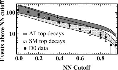
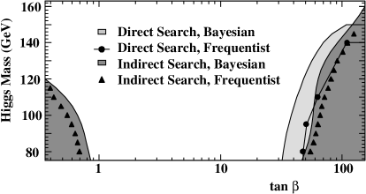
Figure 29: Search for the $H^{\pm}$ at DØ in Run I [290]. (a) The number of observed events in data versus the cut on the neural network output (dots). Overlaid is the expectation from the SM (light shaded area) and a scenario with additional $H^{\pm}$ production in top quark decays for $\tan\beta=150$ and $M_{H^{\pm}}=95\,\mathrm{GeV}/c^{2}$. (b) Exclusion region at the 95% confidence level in $(M_{H^{\pm}},\tan\beta)$ space. The top quark mass is assumed to be 175 GeV/$c^{2}$ and $\sigma(t\bar{t})=5.5\,\mathrm{pb}$. The plot also contains the regions excluded by the indirect search method [289], where DØ looks for a potential disappearance of the $t\bar{t}$ signal.

The data show good agreement with the SM expectation, thereby falsifying the chosen $H^{\pm}$ scenario. Based on a series of Monte Carlo experiments the sensitivity for the $H^{\pm}$ search is optimized yielding on optimal cutoff at 0.91.

After the neural network cut hadronic tau decays are identified in the data. A narrow jet with $\Delta R<0.25$ is required, with 1 to 7 tracks in the jet cone. Events with identified muons or electrons are rejected. In addition, a $\chi^{2}$ requirement is constructed using calorimeter information from $W\rightarrow\tau\nu$ Monte Carlo events. After all cuts $3.2\pm 1.5$ multijet background events are expected, $1.1\pm 0.3$ from $t\bar{t}$ and $0.9\pm 0.3$ from $W+\mathrm{jets}$. In data DØ observes three events. A Bayesian and a Frequentist statistical analysis are used to deduce exclusion regions is the $(M_{H^{\pm}},\tan\beta)$ phase space shown in figure 29b. Under the assumption that $M_{\mathrm{top}}=175\,\mathrm{GeV}/c^{2}$ and $\sigma(t\bar{t})=5.5\,\mathrm{pb}$, the region of $\tan\beta>32.0$ is excluded at the 95% C.L. for $M_{H^{\pm}}=75\,\mathrm{GeV}/c^{2}$. For Higgs masses above 150 GeV/$c^{2}$ no limits can be set. This result can also be interpreted in terms of the branching fraction of $t\rightarrow H^{+}b$, setting a lower limit of $\mathrm{BF}(t\rightarrow H^{+}b)>0.36$ at the 95% C.L..

9.2 Search for $X^{0}\rightarrow t\bar{t}$ decays

Several extensions of the SM predict the existence of narrow resonances that decay to $t\bar{t}$ pairs. One such model is, for example, a $Z^{\prime}$ predicted by top-colour-assisted technicolour [292]. This model speculates that the spontaneous breaking of electroweak symmetry is related to the observed fermion masses, in particular the large top quark mass, and can be accomplished by dynamical effects [293].

CDF and DØ have performed model-independent searches for a narrow resonance $X^{0}$ which decays into a $t\bar{t}$ pair [294, 295]. Both analyses relate closely to the respective top quark mass measurements of the two experiments [224, 243] and employ fits to the invariant mass spectrum of the $t\bar{t}$ pair. DØ obtains a slightly better mass limit. The DØ analysis is based on data with an integrated luminosity of $130\,\mathrm{pb^{-1}}$ and uses events with a lepton-plus-jets signature passing the topological and the soft muon $b$ tag selection. The events are subjected to a kinematic fit that comprises kinematic constraints on the reconstructed $W$ boson mass and the top quark mass. Out of all possible permutations the option with the best $\chi^{2}$ is chosen. The $\chi^{2}$ is required to be below 10. After all cuts 41 events are left in the data sample. Figure 30a shows the invariant mass distribution of the $t\bar{t}$ pair reconstructed from data.

(a)                                                                (b)
   

Figure 30: (a) Invariant mass distribution of the reconstructed $t\bar{t}$ pair of 41 events in the DØ lepton-plus-jets data sample [295]. The solid histogram shows the shape of the $W+$ jets and QCD multijets background, the hatched histogram the sum of all SM backgrounds including $t\bar{t}$ production, and the open histogram shows the sum of signal ($M_{X}=400\,\mathrm{GeV}/c^{2}$) and background as obtained from the fit to the data. (b) Feynman diagram for the FCNC decay $t\rightarrow cZ^{0}$ with $Z\rightarrow e^{+}e^{-}$. Other diagrams involve the $d$ and the $s$ quark within the loop instead of the $b$ quark. All diagrams together nearly cancel and cause the branching ratio of this decay to be very small, $\mathcal{O}(10^{-12})$, in the SM.

The data are fit to distributions for the combined QCD multijet and $W+$ jets background, SM $t\bar{t}$ production, and a signal for $X^{0}\rightarrow t\bar{t}$. For comparison to the data figure 30a shows the backgrounds and the signal component ($M_{X}=400\,\mathrm{GeV}/c^{2}$) obtained from the fit. There is no significant deviation from the SM prediction. The fit is repeated for several assumptions for the $X^{0}$ mass, again without providing evidence for a signal. Therefore, upper limits on the $X^{0}$ production cross section times branching ratio to $t\bar{t}$ are set, ranging from 5.0 pb at $M_{X}=400\,\mathrm{GeV}/c^{2}$ to 1.5 pb at $M_{X}=850\,\mathrm{GeV}/c^{2}$. The confidence level is 95%. These limits are valid as long as the width of the resonance, $\Gamma_{X}$, is small compared to the DØ detector resolution. The limits quoted above assume a width of $\Gamma_{X}=0.012\,M_{X}$. If one compares the cross section limits with the predictions for a leptophobic $Z^{\prime}$ boson, one can obtain a lower limit on the $Z^{\prime}$ mass: $M_{Z^{\prime}}>560\,\mathrm{GeV}/c^{2}$.

9.3 FCNC decays

In the SM flavour changes at leading order (tree level) are induced by charged currents, the exchange of $W$ bosons. Flavour changing neutral currents (FCNC) are only possible at higher orders in perturbation theory (loop level). FCNC decays of the top quark are strongly suppressed in the SM due to the Glashow-Iliopoulos-Maiani (GIM) mechanism [296]. Compared to the top quark mass the masses of down-type quarks ($d$, $s$, $b$) occurring in loop diagrams are small and degenerate. Therefore, the sum over the respective amplitudes nearly cancels. Fig. 30b shows one of the Feynman diagrams that describe the decay $t\rightarrow cZ^{0}$. This type of diagram is also called penguin diagram. The SM predicts the branching fractions for $t\rightarrow cZ^{0}$ and $t\rightarrow c\gamma$ to be on the order of $10^{-12}$, while $\mathrm{BF}(t\rightarrow cg)\simeq 10^{-10}$ and $\mathrm{BF}(t\rightarrow cH^{0})\simeq 10^{-13}$ [297].

In extensions of the SM FCNC top quark decays can be considerably enhanced by several orders of magnitude if FCNC couplings at tree level are allowed [298, 299, 300]. In Two Higgs Doublet Models where the neutral scalar $h^{0}$ posses flavor changing couplings the decay $t\rightarrow ch^{0}$ can be considerably enhanced [301]. A similar enhancement can be reached in supersymmetric models were $R$-parity is violated [302]. In topcolour-assisted technicolour theories the branching ratio for $t\rightarrow cW^{+}W^{-}$ can reach values up to $10^{-3}$ [303]. Since the SM predictions for FCNC interactions have much smaller rates, they are useful probes for new physics beyond the SM.

The CDF collaboration has searched for the FCNC decays $t\rightarrow qZ^{0}$ and $t\rightarrow q\gamma$ in Run I data with an integrated luminosity of $110\,\mathrm{pb^{-1}}$ [304]. The $Z^{0}$ is measured in the decay channels $e^{+}e^{-}$ or $\mu^{+}\mu^{-}$. Electron and muon identification is described in section 4.5.1. A Photon is identified as an energy cluster in the electromagnetic calorimeter with no track pointing at it. Additionally, a cluster with a single soft track pointing to it is accepted as a photon, if the track carries less than 10% of the cluster energy. A typical photon cluster consists of two adjacent towers in the electromagnetic calorimeter. The direction of the photon is defined by the line between the event vertex and the centroid of the electromagnetic shower as measured in the shower maximum detector. Background from hadronic jets is reduced by demanding that the photon cluster is isolated from other energy depositions in the electromagnetic or the hadron calorimeter. In addition, the ratio of hadronic to electromagnetic energy is constrained to be less than $0.055+0.00045\,E$, where $E$ is the sum of hadronic and electromagnetic energy of the cluster measured in the calorimeter.

The search strategy for the FCNC decays tries to isolate $t\bar{t}$ events where one top quark decays via FCNC and the second top quark decays according to the SM decay $t\rightarrow W^{+}b$. In the $t\rightarrow q\gamma$ search two signatures are considered, where the $W$ boson decays either leptonically into $e\nu_{e}$ or $\mu\nu_{\mu}$ or hadronically into quarks. In the first subsample a well identified charged lepton ($e$ or $\mu$) with $p_{\mathrm{T}}>20\,\mathrm{GeV}/c$, $E_{\mathrm{T}}\!\!\!\!\!\!\!/\ \;>20\,\mathrm{GeV}$, a photon with $E_{\mathrm{T}}>20\,\mathrm{GeV}$, and at least two jets with $E_{\mathrm{T}}>15\,\mathrm{GeV}$ are required. The second subsample contains events with at least four jets and one photon with $E_{\mathrm{T}}>50\,\mathrm{GeV}$. At least one jet must be identified as a $b$ quark jet with a secondary vertex tag. In both subsamples, there must be a photon-plus-jet combination with an invariant mass in the top quark mass window $140<M_{j\gamma}<210\,\mathrm{GeV}/c^{2}$. In the hadronic subsample, the remaining jets must have $\sum E_{\mathrm{T}}\geq 140\,\mathrm{GeV}$. One event passes all selection criteria. The event features a $72\,\mathrm{GeV}$ muon, $E_{\mathrm{T}}\!\!\!\!\!\!\!/\ \;=24\,\mathrm{GeV}$, a $88\,\mathrm{GeV}$ photon, and three jets. The background is expected to be about 0.5 events, mainly from $W\gamma$ production with two additional jets.

In the $t\rightarrow qZ^{0}$ search, the $W$ from the second top quark decay is considered to decay hadronically, while the $Z^{0}$ is reconstructed in its leptonic decay modes to $e^{+}e^{-}$ or $\mu^{+}\mu^{-}$. This yields an event signature of four jets and two leptons with an invariant mass close to the $Z^{0}$ mass ($75<M_{\ell\ell}<105\,\mathrm{GeV}/c^{2}$). Since the branching ratio of $Z^{0}\rightarrow\ell^{+}\ell^{-}$ is small, the total detection efficiency of the $t\rightarrow qZ^{0}$ mode is much smaller than the one for the $t\rightarrow q\gamma$ search. Each of the four jets must have $E_{\mathrm{T}}>20\,\mathrm{GeV}$ and $|\eta|<2.4$. One $Z\rightarrow\mu^{+}\mu^{-}$ event passes all selection criteria. The expected background is 0.6 events.

Since no statistically significant excess is observed in both searches, the data are used to set upper limits on the top quark branching ratios into FCNC decays

$$\mathrm{BR}\left(t\rightarrow u/c+\gamma\right)<3.2\%\ \ \ \ \ \ \ \ \ \ \ \ \mathrm{BR}\left(t\rightarrow u/c+Z^{0}\right)<33\%$$ (41)

at the $95\%$ confidence level. These limits are still far from the interesting region. At the LHC experiments will reach a sensitivity level of $10^{-4}$ [5], and thereby reach a region where some models predicting very large enhancements can be excluded [305].

9.4 Anomalous single top production

At the Tevatron the search for anomalously enhanced FCNC in top quark decays is statistically restricted by the number of $t\bar{t}$ pairs produced. More stringent limits on anomalous $tq\gamma$ of $tqZ$ couplings at tree level are set by searching for the production of single top quarks via FCNC at LEP and HERA. At LEP all four experiments have searched for the reactions $e^{+}e^{-}\rightarrow t\bar{c}/t\bar{u}$ and presented upper limits on anomalous couplings [306, 307, 308, 309]. The limits obtained by the L3 collaboration are shown in figure 32.

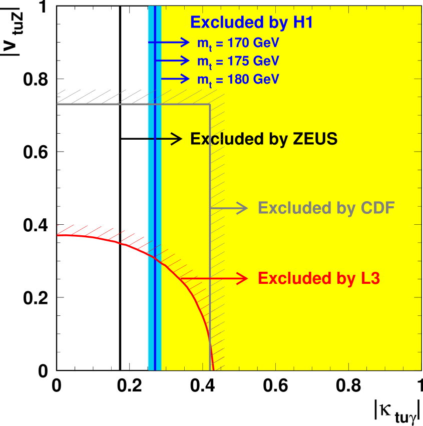
Figure 31: Limits at the 95% confidence level on anomalous couplings $\kappa_{tu\gamma}$ and $\kappa_{tuZ}$ (in this plot noted as $v_{tuZ}$) of the top quark to the $\gamma$ or the $Z$ boson from reference [310]. The plot shows the limits obtained by the HERA experiments H1 and ZEUS [310, 311], by L3 [307] and by CDF [304] (see section 9.3).

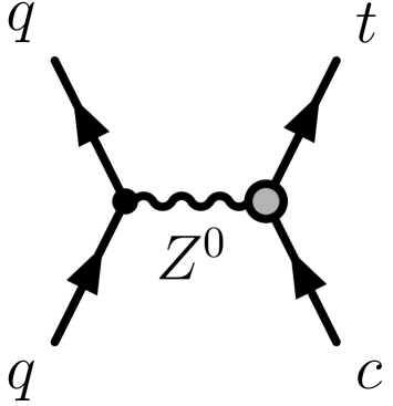
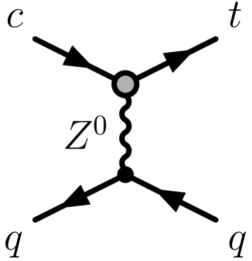
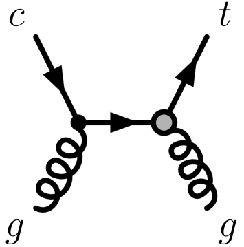
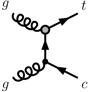
Figure 32: Feynman diagrams for single top production via $2\rightarrow 2$ FCNC processes in hadron collisions.

For $\kappa_{\gamma}=0$ the coupling to the $tqZ$ coupling is constrained by $\kappa_{Z}<0.41$, for $\kappa_{Z}=0$ the $tq\gamma$ coupling is confined to $\kappa_{\gamma}<0.49$. Both limits are taken at the 95% confidence level. The other LEP collaborations obtain very similar results. Figure 32 also visualises the limits that result from the CDF analysis discussed in section 9.3. The LEP results can be translated into limits on the branching ratios: $\mathrm{BR}(t\rightarrow u/c+\gamma)<4.2\%$ and $\mathrm{BR}(t\rightarrow u/c+Z^{0})<14\%$ [308].

At HERA the two experiments H1 and ZEUS searched for top quarks produced in the inclusive FCNC reaction $ep\rightarrow etX$ [310, 311]. The SM process for single top production at HERA is the charged current reaction $ep\rightarrow\nu t\bar{b}X$ [312] with a predicted cross section of less than 1 fb [113], well below the sensitivity of the experiments. An observed excess in this channel can therefore signal physics beyond the SM. ZEUS has analyzed a data sample corresponding to $130\,\mathrm{pb^{-1}}$ of integrated luminosity. The top quark is assumed to decay according to the SM decay $t\rightarrow W^{+}b$. The $W$ boson is detected in its leptonic and the hadronic decays channels. The observed data are in good agreement with the background expectation. Thus, ZEUS is able to compute an upper limit on the anomalous $tu\gamma$ coupling: $\kappa_{tu\gamma}<0.174$ at the 95% confidence level, which is the best limit on this quantity to date. The ZEUS result is depicted in figure 32.

The H1 analysis uses data with an integrated luminosity of $118.3\,\mathrm{pb^{-1}}$ [310]. In the leptonic channel five events are observed over a SM background of $1.31\pm 0.22$. If this excess is attributed to FCNC top quark production a total cross section of $\sigma(ep\rightarrow etX)=0.29^{+0.15}_{-0.14}\,\mathrm{pb}$ is found. In the hadronic channel there is no excess in the data. Only more data will help to decide whether the observation is a real signal or just a statistical fluctuation.

At the Tevatron there are no searches for anomalous single top quark production yet. Possible FCNC processes at tree level could be $q_{1}\bar{q}_{1}\rightarrow t\bar{q}_{2}$, $q_{1}\bar{q}_{2}\rightarrow t\bar{q}_{2}$, $qg\rightarrow tg$, and $gg\rightarrow t\overline{q}$. Example Feynman diagrams for these processes are shown in figure 32. Another option for FCNC top quark production is the $2\rightarrow 1$ quark-gluon fusion process $g+u/c\rightarrow t$. Studies at parton level suggest that the anomalous up quark coupling parameter $\kappa_{tug}/\Lambda$ can be measured down to $0.02~{}\mathrm{TeV^{-1}}$ in Run II of the Tevatron [275]. For the anomalous charm quark coupling parameter $\kappa_{tcg}/\Lambda$ a bound of $0.06~{}\mathrm{TeV^{-1}}$ is in reach. Studies with a fast detector simulation for ATLAS indicate a similar reach at the LHC [313].

10 Summary and outlook

Ten years after the discovery of the top quark many of its properties have been thoroughly investigated. All measurements are in good agreement with the predictions made by the Standard Model (SM). At the Tevatron and at LHC the production of $t\bar{t}$ pairs is the dominating source of top quarks. The experiments CDF and DØ have established $t\bar{t}$ signals in the dilepton, the lepton-plus-jets and the all hadronic channels and measured the production cross section. The $t\bar{t}$ channels involving tau leptons have not been observed yet, but they are well within reach in Run II at the Tevatron.

The most important parameter of the top quark is its mass. The large value of $M_{\mathrm{top}}$ distinguishes the top quark strongly from the other quarks, since it decays essentially as a free quark. Thus, the top quark is an ideal laboratory to study polarization effects in heavy quark production and decay. Via higher order perturbative corrections the top quark mass is strongly correlated with the $W$ boson mass and the Higgs boson mass. Therefore, electroweak precision tests and predictions of $M_{H}$ are very sensitive to $M_{\mathrm{top}}$. The final combined Run I result on the top quark mass yields: $M_{\mathrm{top}}=(178.0\pm 4.3)\,\mathrm{GeV}/c^{2}$. Run II measurements are underway. First preliminary measurements indicate a slightly lower mass value. CDF finds $M_{\mathrm{top}}=173.5^{+2.7}_{-2.6}\,(\mathrm{stat.})\pm 2.5\,(\mathrm{JES})\pm 1.7\,(\mathrm{syst.})\,\mathrm{GeV}/c^{2}$, DØ $M_{\mathrm{top}}=170.6\pm 4.2\,(\mathrm{stat.})\pm 6.0\,(\mathrm{syst.})\,\mathrm{GeV}/c^{2}$. At the end of Run II the top quark mass will be measured with an uncertainty of $2\;\mathrm{to}\;3\,\mathrm{GeV}/c^{2}$. At the LHC the precision of $M_{\mathrm{top}}$ will reach about 1 GeV$/c^{2}$. A limiting factor will be the theoretical understanding of the relation between the kinematic quark mass measured by experiments and the theoretically well defined pole mass or $\mathrm{\overline{MS}}$ mass. The final word on $M_{\mathrm{top}}$ will come from an $e^{+}e^{-}$ linear collider where a scan of the $t\bar{t}$ production threshold will allow for a precision of about $20\,\mathrm{MeV}/c^{2}$.

After the discovery of the top quark the focus of research by the CDF and DØ collaborations shifted to a detailed investigation of its production and decay properties. The helicity of $W$ bosons from the top quark decay was measured and found to agree with the SM $V-A$ theory of the electroweak interaction. The ratio of branching ratios $R_{tb}=\mathrm{BF}(t\rightarrow Wb)/\mathrm{BF}(t\rightarrow Wq)$ was determined and found to agree with a value close to 1 as predicted by the SM. DØ has investigated $t\bar{t}$ dilepton events for spin correlations among the two charged leptons, CDF has measured the top quark $p_{\mathrm{T}}$ spectrum. Both analyses show no significant deviations from the SM. The search for electroweak single top quark production is about to reach a critical phase in Run II. A discovery of this top quark production mode is around the corner.

Its large mass is motivation to view the top quark as an ideal probe for new physics beyond the SM. Already before the top quark discovery the search for the decay $t\rightarrow H^{+}b$ started. CDF and DØ searched also for a heavy resonance which decays into a $t\bar{t}$ pair. A CDF analysis looked for FCNC decays of the top quark. No indication of these phenomena beyond the SM is found.

The LHC will be a top quark factory where several millions of top quarks will be produced per year. This wealth of data will allow to enter a precision era of top quark physics where top quark properties will be very accurately investigated. The Tevatron analyses provide an excellent basis for further studies at the LHC. But also new topics where huge amounts of data are needed will become accessible at the LHC, for example, the search for like sign top pair production ($tt$ or $\bar{t}\bar{t}$), production of single top quarks via FCNC, the search for $CP$ violation in $t\bar{t}$ production, or the direct measurement of the electric charge of the top quark. The abundance of analysis topics and open questions guarantees that top quark physics will remain a lively and thrilling field of elementary particle research in the coming years which will see the end of Run II at the Tevatron and the turn on of the LHC.

References

References

- [1] Azzi P et al 2004 Preprint hep-ex / 0404010
- [2] Peccei R D, Peris S and Zhang X 1991 Nucl. Phys. B 349 305–322
- [3] Mangano M and Trippe T 2004 Phys. Lett. B 592 483
- [4] Chakraborty D, Konigsberg J and Rainwater D L 2003 Ann. Rev. Nucl. Part. Sci. 53 301–351
- [5] Ahmadov A et al 2000 Preprint hep-ph / 0003033
- [6] Bhat P C, Prosper H and Snyder S S 1998 Int. J. Mod. Phys. A 13 5113–5218
- [7] Campagnari C and Franklin M 1997 Rev. of Mod. Phys. 669 137
- [8] Kühn J H 1997 Preprint hep-ph / 9707321
- [9] Teubner T 1999 Acta Phys. Polon. B 30 1941–1966
- [10] Eidelman S et al 2004 Phys. Lett. B 592 1
- [11] Barger V D and Phillips R J N Collider Physics Frontiers in physics. Addison-Wesley Reading 1987
- [12] Halzen F and Martin A D Quarks & leptons John Wiley & Sons New York 1984
- [13] Griffiths D J Introduction to elementary particles John Wiley & Sons New York 1987
- [14] Perkins D H Introduction to high energy physics Addison-Wesley Reading 1987
- [15] Lohrmann E Hochenergiephysik Teubner Stuttgart 1992
- [16] Fukuda S et al 2002 Phys. Lett. B 539 179–187
- [17] Ahmad Q R et al 2001 Phys. Rev. Lett. 87 071301
- [18] Ahmad Q R et al 2002 Phys. Rev. Lett. 89 011301
- [19] Glashow S L 1961 Nucl. Phys. 22 579–588
- [20] Weinberg S 1967 Phys. Rev. Lett. 19 1264–1266
- [21] Salam A Elementary particle theory: relativistic groups and analyticity In Svartholm N, editor, Nobel symposium No. 8 page 367 Stockholm 1968. Almquist and Wiksell
- [22] Goldstone J 1961 Nuovo Cim. 19 154–164
- [23] Goldstone J, Salam A and Weinberg S 1962 Phys. Rev. 127 965–970
- [24] Kobayashi M and Maskawa K 1973 Prog. Theor. Phys. 49 652–657
- [25] Perl M L et al 1975 Phys. Rev. Lett. 35 1489–1492
- [26] Herb S W et al 1977 Phys. Rev. Lett. 39 252
- [27] Berger C et al 1978 Phys. Lett. B 76 243–245
- [28] Bienlein J K et al 1978 Phys. Lett. B 78 360–363
- [29] Darden C W et al 1978 Phys. Lett. B 76 246
- [30] Bartel W et al 1984 Phys. Lett. B 146 437–442
- [31] ‘t Hooft G 1971 Nucl. Phys. B 33 173–199
- [32] ‘t Hooft G 1971 Nucl. Phys. B 35 167–188
- [33] Leader E and Pedrazzi E An introduction to gauge theories and the new physics page 76 Cambridge University Press Cambridge, UK 1982
- [34] Langacker P 1989 Phys. Rev. Lett. 63 1920
- [35] Hollik W F L 1990 Fortschr. Phys. 38 165–260
- [36] Myers S and Picasso E 1990 Contemp. Phys. 31 387–403
- [37] Decamp D et al 1990 Nucl. Instr. and Meth. A 294 121–178
- [38] Buskulic D et al 1995 Nucl. Instr. and Meth. A 360 481–506
- [39] Aarnio P A et al 1991 Nucl. Instr. and Meth. A 303 233–276
- [40] Abreu P et al 1996 Nucl. Instr. and Meth. A 378 57–100
- [41] Acciarri M et al 1994 Nucl. Instr. and Meth. A 351 300–312
- [42] Adam A et al 1996 Nucl. Instr. and Meth. A 383 342–366
- [43] Ahmet K et al 1991 Nucl. Instr. and Meth. A 305 275–319
- [44] Richter B 1990 Part. Accel. 26 33–50
- [45] Agnew G et al 1984 SLAC public note 0273
- [46] Suekane F et al 1997 Nucl. Instr. and Meth. A 386 46–51
- [47] Abbaneo D et al 2004 Preprint hep-ex / 0412015
- [48] Schaile D 1994 Fortsch. Phys. 42 429–484
- [49] Quast G 1999 Prog. Part. Nucl. Phys. 43 87–166
- [50] Abbaneo D et al 2003 Phys. Lett. B 565 61
- [51] Albajar C et al 1987 Phys. Lett. B 186 247
- [52] Albrecht H et al 1987 Phys. Lett. B 192 245
- [53] Heister A et al 2003 Eur. Phys. J. C 29 143
- [54] Abdallah J et al 2003 Eur. Phys. J. C 28 155
- [55] Abbiendi G et al 2001 Eur. Phys. J. C 19 241
- [56] Abe K et al 2003 Phys. Rev. D 67 012006
- [57] Abe F et al 1999 Phys. Rev. Lett. 82 3576–3580
- [58] Link J M et al 2000 Phys. Lett. B 485 62–70 hep-ex/0004034
- [59] Link J M 2001 Preprint hep-ex / 0106093
- [60] Palmer M A 2001 Int. Jour. of Mod. Phys. A 16, Suppl. 1B 520–523
- [61] Aubert B et al 2003 Phys. Rev. Lett. 91 171801
- [62] Cheng H Y 1982 Phys. Rev. D 26 143–160
- [63] Chau L L 1983 Phys. Rept. 95 1
- [64] Buras A J, Slominski W and Steger H 1984 Nucl. Phys. B 245 369–398
- [65] Inami T and Lim C S 1981 Progr. Theor. Phys. 65 297 Erratum: 1981 65 1772
- [66] Buras A J and Fleischer R In Buras A J and Lindner M, editors, Heavy Flavours II. World Scientific Singapore 1998
- [67] Buras A J, Jamin M and Weisz P H 1990 Nucl. Phys. B 347 491–536
- [68] Ellis J, Hagelin J S and Rudaz S 1987 Phys. Lett. B 192 201
- [69] Bigi I I and Sanda A I 1987 Phys. Lett. B 194 307
- [70] Barger V D, Han T and Nanopoulos D V 1987 Phys. Lett. B 194 312
- [71] Datta A, Paschos E A and Türke U 1987 Phys. Lett. B 196 376
- [72] Du D S and Zhao Z Y 1987 Phys. Rev. Lett. 59 1072–1075
- [73] Collins J C, Soper D E and Sterman G 1986 Nucl. Phys. B 263 37–60
- [74] Abt I et al 1997 Nucl. Instr. and Meth. A 386 310–347
- [75] Lai H L et al 1995 Phys. Rev. D 51 4763–4782
- [76] Berger E L and Contopanagos H 1998 Phys. Rev. D 57 253–264
- [77] Bonciani R, Catani S, Mangano M L and Nason P 1998 Nucl. Phys. B 529 424
- [78] Laenen E, Smith J and van Neerven W L 1994 Phys. Lett. B 321 254–258
- [79] Glück M, Owens J F and Reys E 1978 Phys. Rev. D 17 2324–2331
- [80] Jones L M and Wyld H W 1978 Phys. Rev. D 17 1782–1787
- [81] Babcock J, Sivers D and Wolfram S 1977 Phys. Rev. D 18 162–181
- [82] Georgi H M, Glashow S L, Machacek M E and Nanopoulos D V 1978 Ann. Phys. 114 273–289
- [83] Combridge B L 1979 Nucl. Phys. B 151 429–456
- [84] Hagiwara K and Yoshino T 1979 Phys. Lett. B 80 282–285
- [85] Nason P, Dawson S and Ellis R K 1988 Nucl. Phys. B 303 607–633
- [86] Beenakker W, Kuijf H, van Neerven W L and Smith J 1989 Phys. Rev. D 40 54–82
- [87] Beenakker W, van Neerven W L, Meng R, Schuler G A and Smith J 1991 Nucl. Phys. B 351 507–560
- [88] Nason P, Dawson S and Ellis R K 1989 Nucl. Phys. B 327 49–92 Erratum: 1990 Nucl. Phys. B 335 260
- [89] Altarelli G, Diemoz M, Martinelli G and Nason P 1988 Nucl. Phys. B 308 724–752
- [90] Ellis R K 1991 Phys. Lett. B 259 492–496
- [91] Cacciari M, Frixione S, Mangano M L, Nason P and Ridolfi G 2004 JHEP 0404 068
- [92] Laenen E, Smith J and van Neerven W L 1992 Nucl. Phys. B 369 543–599
- [93] Berger E L and Contopanagos H 1995 Phys. Lett. B 361 115–120
- [94] Berger E L and Contopanagos H 1996 Phys. Rev. D 54 3085–3113
- [95] Catani S, Mangano M L, Nason P and Trentadue L 1996 Phys. Lett. B 378 329–336
- [96] Catani S, Mangano M L, Nason P and Trentadue L 1996 Nucl. Phys. B 478 273–310
- [97] Kidonakis N, Laenen E, Moch S and Vogt R 2001 Phys. Rev. D 64 114001
- [98] Kidonakis N 2001 Phys. Rev. D 64 014009
- [99] Kidonakis N and Vogt R 2003 Phys. Rev. D 68 114014
- [100] Stump D R et al 2002 Phys. Rev. D 65 014012
- [101] Pumplin J et al 2002 Phys. Rev. D 65 014013
- [102] Martin A D, Roberts R G, Stirling W J and Thorne R S 2002 Preprint hep-ph / 0211080
- [103] Affolder T et al 2001 Phys. Rev. D 64 032002
- [104] Affolder T et al 2001 Phys. Rev. D 63 32003
- [105] Abazov V M et al 2003 Phys. Rev. D 67 012004
- [106] Abazov V M et al 2004 Nature 429 638
- [107] Heinson A P, Belyaev A S and Boos E E 1997 Phys. Rev. D 56 3114–3128
- [108] Anselmo F, van Eijk B and Bordes G 1992 Phys. Rev. D 45 2312–2322
- [109] Willenbrock S S D and Dicus D A 1986 Phys. Rev. D 34 155–161
- [110] Dawson S and Willenbrock S S D 1987 Nucl. Phys. B 284 449–462
- [111] Yuan C P 1990 Phys. Rev. D 41 42–51
- [112] Bordes G and van Eijk B 1995 Nucl. Phys. B 435 23–58
- [113] Stelzer T, Sullivan Z and Willenbrock S S D 1997 Phys. Rev. D 56 5919–5927
- [114] van der Heide J, Laenen E, Laenen L and Weinzierl S 2000 Phys. Rev. D 62 074025
- [115] Stelzer T, Sullivan Z and Willenbrock S S D 1998 Phys. Rev. D 58 094021
- [116] Harris B W, Laenen E, Phaf L, Sullivan Z and Weinzierl S 2002 Phys. Rev. D 66 054024
- [117] Sullivan Z 2004 Phys. Rev. D 70 114012
- [118] Tait T M P 1999 Phys. Rev. D 61 34001
- [119] Carlson D and Yuan C P 1993 Phys. Lett. B 306 386–390
- [120] Mahlon G and Parke S 1997 Phys. Rev. D 55 7249–7254
- [121] Cortese S and Petronzio R 1991 Phys. Lett. B 253 494–498
- [122] Smith M C and Willenbrock S S D 1996 Phys. Rev. D 54 6696–6702
- [123] Mrenna S and Yuan C P 1998 Phys. Lett. B 416 200
- [124] Belyaev A and Boos E 2001 Phys. Rev. D 63 034012
- [125] Boos E E et al 1995 Preprint hep-ph / 9503280
- [126] Fischer M, Groote S, Korner J G and Mauser M C 2001 Phys. Rev. D 63 031501
- [127] Fischer M, Groote S, Korner J G and Mauser M C 2002 Phys. Rev. D 65 054036
- [128] Do H S, Groote S, Korner J G and Mauser M C 2003 Phys. Rev. D 67 091501
- [129] Jezabek M and Kühn J H 1989 Nucl. Phys. B 314 1–6
- [130] Jezabek M and Kühn J H 1988 Phys. Lett. B 207 91–96
- [131] Bigi I I, Dokshitzer Y, Khoze V, Kühn J H and Zerwas P 1986 Phys. Lett. B 181 157–163
- [132] Czarnecki A and Melnikow K 1999 Nucl. Phys. B 544 520–531
- [133] Chetyrkin K G, Harlander R, Seidensticker T and Steinhauser M 1999 Phys. Rev. D 60 114015
- [134] Fadin V S, Khoze V A and Martin A D 1994 Phys. Rev. D 49 2247–2256
- [135] Mrenna S and Yuan C P 1992 Phys. Rev. D 46 1007–1021
- [136] Denner A and Sack T 1991 Nucl. Phys. B 358 46
- [137] Migneron R, Eilam G, Mendel R R and Soni A 1991 Phys. Rev. Lett. 66 3105
- [138] Jezabek M and Kühn J H 1993 Phys. Rev. D 48 R1910 Erratum: 1994 Phys. Rev. D 49 4970
- [139] Kühn J H 1981 Act. Phys. Pol. B 12 347
- [140] Kühn J H 1982 Act. Phys. Austr. Suppl. XXIV 203
- [141] Orr L H 1991 Phys. Rev. D 44 88–98
- [142] Jezabek M and Kühn J H 1994 Phys. Lett. B 329 317–324
- [143] Mahlon G 1998 Preprint hep-ph / 981121
- [144] Garbincius P L 2004 Preprint hep-ex / 0406013
- [145] Acosta D et al 2005 Phys. Rev. D 71 032001
- [146] Abe F et al 1988 Nucl. Instr. and Meth. A 271 387–403
- [147] Abe F et al 1995 Phys. Rev. D 52 4784–4827
- [148] Affolder T et al 2004 Nucl. Instr. and Meth. A 526 249
- [149] Sill A et al 2000 Nucl. Instr. and Meth. A 447 1
- [150] Affolder A et al 2000 Nucl. Instr. and Meth. A 453 84–88
- [151] Acosta D et al 2004 Nucl. Instr. and Meth. A 518 605
- [152] Balka L et al 1988 Nucl. Instr. and Meth. A 267 272–279
- [153] Albrow M et al 2002 Nucl. Instr. and Meth. A 480 524–546
- [154] Bertolucci S et al 1988 Nucl. Instr. and Meth. A 267 301–314
- [155] Ascoli G et al 1988 Nucl. Instr. and Meth. A 268 33
- [156] Acosta D et al 2001 Nucl. Instr. and Meth. A 461 540–544
- [157] Quinn B 2003 Nucl. Instr. and Meth. A 501 7–13
- [158] Bross A et al 1998 AIP Conf. Proc. 450 221–228
- [159] Gordeev A et al 2003 Fermilab public note 98-416-E
- [160] Acharya B S et al 1997 Nucl. Instr. and Meth. A 401 45–62
- [161] Abramov V et al 1998 Nucl. Instr. and Meth. A 419 660–666
- [162] Bantly J et al 1994 IEEE Trans. Nucl. Sci. 41 1274–1279
- [163] Hu Y et al 2004 IEEE Trans. Nucl. Sci. 51 2368–2372
- [164] Linnemann J T 2001 Int. J. Mod. Phys. A 16S1C 1166–1168
- [165] Miao C C 1999 Nucl. Phys. Proc. Suppl. 78 342–347
- [166] Abe F et al 1994 Phys. Rev. D 50 2966
- [167] Abachi S et al 1995 Phys. Rev. D 52 4877
- [168] Acosta D et al 2005 Phys. Rev. D 71 052003
- [169] Abazov V M et al 2005 Phys. Rev. Lett. 94 161801
- [170] Abazov V M et al 2005 Phys. Rev. Lett. 94 152002
- [171] Sjöstrand T 2001 Comp. Phys. Commun. 135 238
- [172] Marchesini G et al 1992 Comp. Phys. Comun. 67 465
- [173] Gribov V N and Lipatov L N 1972 Sov. J. Nucl. Phys. 15 438
- [174] Dokshitzer Y L 1977 Sov. Phys. JETP 46 641
- [175] Altarelli G and Parisi G 1977 Nucl. Phys. B 126 297
- [176] Frixione S, Mangano M L, Nason P and Ridolfi G 1995 Phys. Lett. B 351 555
- [177] Berends F A, Kuijf H, Tausk B and Giele W T 1991 Nucl. Phys. B 357 32–64
- [178] Mangano M L, Moretti M, Piccinini F, Pittau R and Polosa A 2003 JHEP 07 001
- [179] Brun R and Carminati F 1993 CERN Programming Library Long Writeup W5013
- [180] Pakvasa S and Sugawara H 1979 Phys. Lett. B 82 105
- [181] Preparata G 1979 Phys. Lett. B 82 398
- [182] Mahanthappa K T and Sher M A 1979 Phys. Lett. B 86 294
- [183] Behrend H J et al 1984 Phys. Lett. B 144 297
- [184] Bartel W et al 1981 Phys. Lett. B 99 277
- [185] Adeva B et al 1985 Phys. Lett. B 152 439
- [186] Berger C et al 1979 Phys. Lett. B 86 413
- [187] Althoff M et al 1984 Phys. Lett. B 138 441
- [188] Sagawa H et al 1988 Phys. Rev. Lett. 60 93
- [189] Abe K et al 1990 Phys. Lett. B 234 382
- [190] Decamp D et al 1990 Phys. Lett. B 236 511
- [191] Abreu P et al 1990 Phys. Lett. B 242 536
- [192] Akrawy M Z et al 1990 Phys. Lett. B 236 364
- [193] Abrams S et al 1989 Phys. Rev. Lett. 63 2447
- [194] Arnison G et al 1984 Phys. Lett. B 147 493
- [195] Albajar C et al 1988 Z. Phys. C 37 505
- [196] Albajar C et al 1990 Z. Phys. C 48 1
- [197] Akesson T et al 1990 Z. Phys. C 46 179
- [198] Abe F et al 1990 Phys. Rev. Lett. 64 142
- [199] Abe F et al 1991 Phys. Rev. D 43 664
- [200] Abe F et al 1990 Phys. Rev. Lett. 64 147
- [201] Abe F et al 1992 Phys. Rev. Lett. 68 447
- [202] Abe F et al 1992 Phys. Rev. D 45 3921
- [203] Abachi S et al 1994 Phys. Rev. Lett. 72 2138
- [204] Abe F et al 1994 Phys. Rev. Lett. 73 225
- [205] Abe F et al 1995 Phys. Rev. Lett. 74 2626
- [206] Abachi S et al 1995 Phys. Rev. Lett. 74 2422
- [207] Abachi S et al 1995 Phys. Rev. Lett. 74 2632
- [208] Abe F et al 1995 Phys. Rev. D 51 4623
- [209] Abe F et al 1995 Phys. Rev. D 52 2605
- [210] Brandelik R et al 1982 Phys. Lett. B 113 499
- [211] Adeva B et al 1983 Phys. Rev. Lett. 50 799
- [212] Yoshia H et al 1987 Phys. Lett. B 198 570
- [213] Glashow S L 1980 Phys. Rev. Lett. 45 1914
- [214] Pinna G M 1984 Phys. Lett. B 146 78
- [215] Kubo J, Sibold K and Zimmermann W 1985 Nucl. Phys. B 259 331
- [216] Just K and The L S 1986 Z. Naturforsch. 42a 241
- [217] Alhendi H, Özer M and Taha M O 1988 Phys. Lett. B 213 337
- [218] Marciano W J 1989 Phys. Rev. Lett. 62 2793
- [219] Ellis J and Fogli G L 1990 Phys. Lett. B 249 543
- [220] Bernabeu J, Pich A and Santamaria A 1991 Nucl. Phys. B 363 326
- [221] Arnaudon L et al 1993 Phys. Lett. B 307 187
- [222] Abbaneo D et al 1996 CERN-PPE 96-183
- [223] Abbaneo D et al 2001 CERN-EP 2001-021
- [224] Abe F et al 1998 Phys. Rev. Lett. 80 2767–2772
- [225] Abachi S et al 1997 Phys. Rev. Lett. 79 1197–1202
- [226] Abbott B et al 1999 Phys. Rev. D 60 052001
- [227] Acosta D et al 2004 Phys. Rev. Lett. 93 142001
- [228] Acosta D et al 2005 Phys. Rev. D 72 052003
- [229] Ellis S D et al 1985 Phys. Lett. B 154 435
- [230] Berends F A et al 1991 Nucl. Phys. B 357 32
- [231] Abachi S et al 1995 Phys. Rev. Lett. 75 3226
- [232] Acosta D et al 2004 CDF public note No. 7236
- [233] Acosta D et al 2005 Phys. Rev. D 72 032002
- [234] Abazov V M et al 2004 DØ public note No. 4428
- [235] Abe F et al 1998 Phys. Rev. Lett. 80 2779–2784
- [236] Abe F et al 1997 Phys. Rev. Lett. 79 1992–1997
- [237] Acosta D et al 2004 CDF public note No. 7192
- [238] Abazov V M et al 2004 DØ public note
- [239] Abazov V M et al 2004 DØ public note No. 4528
- [240] Abazov V M et al 2005 Phys. Lett. B 626 35–44
- [241] Acosta D et al 2005 Phys. Rev. D 71 072005
- [242] Abulencia A et al 2006 Phys. Rev. D 74 072005
- [243] Abbott B et al 1998 Phys. Rev. D 58 052001
- [244] Abachi S et al 1997 Phys. Rev. Lett. 79 1203
- [245] Kondo K et al 1993 J. Phys. Soc. Jap. 62 1177
- [246] Dalitz R H and Goldstein G R 1992 Phys. Lett. B 287 225
- [247] Dalitz R H and Goldstein G R 1999 Proc. Roy. Soc. Lond. A 455 2803
- [248] Abe F et al 1999 Phys. Rev. Lett. 82 271–276
- [249] Abazov V M et al 2005 Phys. Lett. B 606 25
- [250] Abbott B et al 1998 Phys. Rev. Lett. 80 2063–2068
- [251] Abazov V M et al 2005 DØ public note No. 4728
- [252] Affolder T et al 2000 Phys. Rev. Lett. 84 216
- [253] Abulencia A et al 2006 Phys. Rev. D 73 111103
- [254] Abazov V M et al 2005 Phys. Lett. B 617 1–10
- [255] Acosta D et al 2005 Phys. Rev. D 71 031101 Erratum: 2005 Phys. Rev. D 71 059901
- [256] Affolder T et al 2001 Phys. Rev. Lett. 86 3233
- [257] Acosta D et al 2005 Phys. Rev. Lett. 95 102002
- [258] Abazov V M et al 2004 DØ public note No. 4586
- [259] Abulencia A et al 2006 Phys. Lett. B 639 172
- [260] Abe F et al 1997 Phys. Rev. Lett. 79 3585
- [261] Mahlon G and Parke S 1997 Phys. Lett. B 411 173
- [262] Mahlon G and Parke S 1996 Phys. Rev. D 53 4886
- [263] Abbott B et al 2000 Phys. Rev. Lett. 85 256
- [264] Affolder T et al 2001 Phys. Rev. Lett. 87 102001
- [265] Acosta D et al 2005 Phys. Rev. D 71 012005
- [266] Abbott B et al 2000 Phys. Rev. D 63 031101
- [267] Abazov V M et al 2001 Phys. Lett. B 517 282–294
- [268] Acosta D et al 2002 Phys. Rev. D 65 091102
- [269] Acosta D et al 2004 Phys. Rev. D 69 052003
- [270] Stelzer T and Long W F 1994 Comput. Phys. Commun. 81 337
- [271] Maltoni F and Stelzer T 2003 J. High Energy Phys. 02 027
- [272] Campbell J M and Ellis R K 1999 Phys. Rev. D 60 113006
- [273] Tait T M P and Yuan C P 2001 Phys. Rev. D 63 014018
- [274] Han T et al 1998 Phys. Rev. D 58 073008
- [275] Hosch M, Whisnant K and Young B L 1997 Phys. Rev. D 56 5725
- [276] Simmons E H 1997 Phys. Rev. D 55 5494
- [277] Rizzo T G 1996 Phys. Rev. D 53 6218
- [278] Malkawi E and Tait T 1995 Phys. Rev. D 54 5758–5762
- [279] Abazov V M et al 2005 Phys. Lett. B 622 265–276
- [280] Albajar C et al 1991 Phys. Lett. B 257 459
- [281] Alitti J et al 1992 Phys. Lett. B 280 137
- [282] Abe F et al 1994 Phys. Rev. Lett. 73 2667
- [283] Abe F et al 1994 Phys. Rev. Lett. 72 1977
- [284] Heister A et al 2001 Preprint hep-ex / 0107031
- [285] Alam M S et al 1995 Phys. Rev. Lett. 74 2885
- [286] Abe F et al 1996 Phys. Rev. D 54 735
- [287] Abe F et al 1997 Phys. Rev. Lett. 79 357
- [288] Affolder T et al 2000 Phys. Rev. D 62 12004
- [289] Abbott B et al 1999 Phys. Rev. Lett. 82 4975
- [290] Abazov V M et al 2002 Phys. Rev. Lett. 88 151803
- [291] Paige F and Protopopescu S 1986 (unpublished) BNL Report No. 38034
- [292] Hill C T and Parke S J 1994 Phys. Rev. D 49 4454
- [293] Bardeen W A, Hill C T and Lindner M 1990 Phys. Rev. D 41 1647
- [294] Affolder T et al 2000 Phys. Rev. Lett. 85 2062
- [295] Abazov V M et al 2004 Phys. Rev. Lett. 92 221801
- [296] Glashow S L, Iliopoulos J and Maiani L 1970 Phys. Rev. D 2 1285–1292
- [297] Eilam G, Hewett J L and Soni A 1991 Phys. Rev. D 44 1473 Erratum: ibidem D59:039901, 1999.
- [298] Fritzsch H 1989 Phys. Lett. B 224 423–425
- [299] Han T, Whisnant K, Young B L and Zhang X 1996 Phys. Lett. B 385 311
- [300] Han T, Peccei R D and Zhang X 1995 Nucl. Phys. B 454 527
- [301] Hou W S 1992 Phys. Lett. B 296 179
- [302] Eilam G, Gemintern A, Han T, Yang J and Zhang X 2001 Phys. Lett. B 510 227
- [303] Yue C, Lu G, Xu Q, Liu G and Gao G 2001 Phys. Lett. B 508 290
- [304] Abe F et al 1998 Phys. Rev. Lett. 80 2525
- [305] Yang J M, Young B L and Zhang X 1998 Phys. Rev. D 58 055001
- [306] Abdallah J et al 2004 Phys. Lett. B 590 21
- [307] Achard P et al 2002 Phys. Lett. B 549 290
- [308] Heister A et al 2002 Phys. Lett. B 543 173
- [309] Abbiendi G et al 2001 Phys. Lett. B 521 181
- [310] Aktas A et al 2004 Eur. Phys. J. C 33 9
- [311] Chekanov S et al 2003 Phys. Lett. B 559 153
- [312] Schuler G A 1988 Nucl. Phys. B 299 21–51
- [313] Cakir O and Cetin S A 2005 J. Phys. G: Nuclear and Particle Physics 31 N1