2005 International Linear Collider Workshop - Stanford, U.S.A.
Dominant Two-Loop Electroweak Correction to $H\to\gamma\gamma$

Abstract

We discuss a recent analysis of a dominant two-loop electroweak correction, of $\mathcal{O}(G_{F}M_{t}^{2})$, to the partial width of the decay of an intermediate-mass Higgs boson into a pair of photons. The asymptotic-expansion technique was used in order to extract the leading dependence on the top-quark mass plus four expansion terms that describe the dependence on the $W$- and Higgs-boson masses. This correction reduces the Born result by approximately 2.5%. As a by-product of this analysis, also the $\mathcal{O}(G_{F}M_{t}^{2})$ correction to the partial width of the Higgs-boson decay to two gluon jets was recovered.

I Introduction

The Higgs boson is the missing link of the Standard Model (SM) of elementary particle physics. If this particle will be discovered at the Fermilab Tevatron or the CERN LHC, then an important experimental task at a future $e^{+}e^{-}$ linear collider (ILC) will be to determine its properties with high precision. The electroweak precision data mainly collected at CERN LEP and SLAC SLC in combination with the direct top-quark mass measurement at the Tevatron favour a Higgs boson with mass $M_{H}=129^{+74}_{-49}$ GeV with an upper bound of about 285 GeV at the 95% confidence level ewwg . Incidentally, this $M_{H}$ window includes the one that is encompassed by the vacuum-stability lower bound and the triviality upper bound allowing the SM to be valid up to the grand-unified-theory scale $\Lambda\approx 10^{16}$ GeV ham . This roughly corresponds to the so-called intermediate mass range, defined by $M_{W}\leq M_{H}\leq 2M_{W}$. In this mass range, the decay into two photons has a branching fraction of up to 0.3% Kniehl:1993ay , represents one of the most useful detection modes at hadron colliders, and produces a clear signal at the ILC. The cross section of $\gamma\gamma\to H$, to be measured in the $\gamma\gamma$ operation mode of the ILC, is proportional to the partial decay width $\Gamma(H\to\gamma\gamma)$. In conclusion, the precise knowledge of $\Gamma(H\to\gamma\gamma)$ is required for $M_{W}\leq M_{H}\leq 2M_{W}$.

Since there is no direct coupling of the Higgs boson to photons, the process $H\to\gamma\gamma$ is loop-induced and so provides a handle on new charged massive particles that are to heavy to be produced on-shell with available particle accelerators. The lowest-order result for $\Gamma(H\to\gamma\gamma)$ has been known for three decades Ellis:1975ap . QCD corrections, which only affect the diagrams involving virtual quarks are known at two Djouadi:1990aj and three Ste96 loops. In Ref. Korner:1995xd , the dominant two-loop electroweak correction for a high-mass Higgs boson was found by means of the Goldstone boson equivalence theorem. In Ref. Djouadi:1997rj , the dominant two-loop electroweak correction induced by a sequential isodoublet of ultraheavy quarks was investigated by means of a low-energy theorem let . Recently, also the two-loop electroweak correction induced by light-fermion loops has been evaluated Aglietti:2004nj . Here, we discuss the two-loop electroweak correction that is enhanced by $G_{F}M_{t}^{2}$ fugel .

Due to electromagnetic gauge invariance, the amputated transition-matrix element of $H\to\gamma\gamma$ possesses the structure

$$\mathcal{T}^{\mu\nu} = (q_{1}\!\cdot\!q_{2}\,g^{\mu\nu}-q_{1}^{\nu}q_{2}^{\mu})\mathcal{A},$$ (1)

where $\mu$ and $\nu$ are the Lorentz indices of the external photons with four-momenta $q_{1}$ and $q_{2}$, respectively. Thus, we have

$$\Gamma(H\to\gamma\gamma)=\frac{M_{H}^{3}}{64\pi}|\mathcal{A}|^{2}.$$ (2)

The form factor $\mathcal{A}$ is evaluated in perturbation theory as

$$\mathcal{A}=\mathcal{A}_{t}^{(0)}+\mathcal{A}_{W}^{(0)}+\mathcal{A}_{tW}^{(1)}+\cdots,$$ (3)

where ${\cal A}_{t}^{(0)}$ and ${\cal A}_{W}^{(0)}$ denote the one-loop contributions induced by virtual top quarks and $W$ bosons, respectively, ${\cal A}_{tW}^{(1)}$ stands for the two-loop electroweak correction involving virtual top quarks, and the ellipsis represents the residual one- and two-loop contributions as well as all contributions involving more than two loops.

Prior to discussing the results for $\mathcal{A}_{t}^{(0)}$, $\mathcal{A}_{W}^{(0)}$, and $\mathcal{A}_{tW}^{(1)}$, we summarize the approximations, techniques, and checks applied in Ref. fugel . For simplicity, the bottom-quark mass is neglected, and the element $V_{tb}$ of the Cabibbo-Kobayashi-Maskawa quark mixing matrix is set to unity, so that the quarks of the third fermion generation decouple from those of the first two, which they actually do to very good approximation Hagiwara:fs . Exploiting the (formal) hierarchy $M_{H}^{2}=2q_{1}\!\cdot\!q_{2}\ll(2M_{W})^{2}\ll M_{t}^{2}$, the method of asymptotic expansion Smirnov:pj is applied to evaluate the results as Taylor expansions in $\tau_{t}=M_{H}^{2}/(2M_{t})^{2}$ and $\tau_{W}=M_{H}^{2}/(2M_{W})^{2}$. The on-mass-shell scheme is adopted, and the ultraviolet (UV) divergences are regularized by means of dimensional regularization. The anti-commuting definition of $\gamma_{5}$ is employed. The tadpole contributions are treated properly. The coefficients of the tensors $q_{1}\!\cdot\!q_{2}\,g^{\mu\nu}$ and $q_{1}^{\nu}q_{2}^{\mu}$ in Eq. (1) are projected out, evaluated separately, and found to agree. The UV divergences are found to cancel in the final result. The general $R_{\xi}$ gauge in adopted for the $W$ boson, and the gauge parameter $\xi_{W}$ is found to drop out in the final result. Terms quartic in $M_{t}$, which arise from the asymptotic expansion, the genuine two-loop tadpoles, and the counterterms are found to cancel. As a by-product of the two-loop calculation, the known result Djouadi:1994ge for the electroweak two-loop correction of $\mathcal{O}(G_{F}M_{t}^{2})$ to $\Gamma(H\to gg)$ is recovered. Finally, the convergence properties of the expansions in $\tau_{t}$ and $\tau_{W}$ are checked.

This presentation is organized as follows. In Sections II, we illustrate the usefulness of the asymptotic-expansion technique by redoing the one-loop calculation. In Section III, we discuss the two-loop calculation. Section IV contains the discussion of the numerical results. We conclude with a summary in Section V.

II One-loop results

Figure 1: Typical one-loop diagrams contributing to $H\to\gamma\gamma$.

Typical Feynman diagrams contributing at one loop in $R_{\xi}$ gauge are depicted in Fig. 1, where $\phi$ and $u$ denote the charged Goldstone bosons and Faddeev-Popov ghosts, respectively. The analytic expression for $\mathcal{A}_{t}^{(0)}$ and $\mathcal{A}_{W}^{(0)}$ in Eq. (3) and their expansions in $\tau_{t}$ and $\tau_{W}$ read:

$$\mathcal{A}_{t}^{(0)} = \hat{\mathcal{A}}N_{c}Q_{t}^{2}\left\{\frac{1}{\tau_{t}}\left[1+\left(1-\frac{1}{\tau_{t}}\right)\arcsin^{2}\sqrt{\tau_{t}}\right]\right\}$$ (4)

$$= \hat{\mathcal{A}}N_{c}Q_{t}^{2}\left(\frac{2}{3}+\frac{7}{45}\tau_{t}+\frac{4}{63}\tau_{t}^{2}+\frac{52}{1575}\tau_{t}^{3}+\frac{1024}{51975}\tau_{t}^{4}+\frac{2432}{189189}\tau_{t}^{5}+\ldots\right),$$

$$\mathcal{A}_{W}^{(0)} = \hat{\mathcal{A}}\left\{-\frac{1}{2}\left[2+\frac{3}{\tau_{W}}+\frac{3}{\tau_{W}}\left(2-\frac{1}{\tau_{W}}\right)\arcsin^{2}\sqrt{\tau_{W}}\right]\right\}$$ (5)

$$= \hat{\mathcal{A}}\left(-\frac{7}{2}-\frac{11}{15}\tau_{W}-\frac{38}{105}\tau_{W}^{2}-\frac{116}{525}\tau_{W}^{3}-\frac{2624}{17325}\tau_{W}^{4}-\frac{640}{5733}\tau_{W}^{5}+\ldots\right),$$

where $\hat{\mathcal{A}}=2^{1/4}G_{F}^{1/2}(\alpha/\pi)$. Here, $\alpha$ is Sommerfeld’s fine-structure constant, $G_{F}$ is Fermi’s constant, $N_{c}=3$ is the number of quark colours, and $Q_{t}=2/3$ is the electric charge of the top quark in units of the positron charge.

III Two-loop results

Figure 2: Typical two-loop electroweak diagrams contributing to $H\to\gamma\gamma$.

The contributions of $\mathcal{O}(G_{F}M_{t}^{2})$ are obtained by considering all two-loop electroweak diagrams involving a virtual top quark. This includes also the tadpole diagrams with a closed top-quark loop, which are proportional to $M_{t}^{4}$. For arbitrary gauge parameter, this leads us to consider a total of order 1000 diagrams. Some of them are depicted in Fig. 2. These diagrams naturally split into two classes. The first class consists of those diagrams where a neutral boson, i.e. a Higgs boson or a neutral Goldstone boson ($\chi$), is added to the one-loop top-quark diagrams. The exchange of a $Z$ boson does not produce quadratic contributions in $M_{t}$. The application of the asymptotic-expansion technique to these diagrams leads to a simple Taylor expansion in the external momenta. This is different for the second class of diagrams, which, next to the top quark, also contain a $W$ or a $\phi$ boson and, as a consequence, also the bottom quark, which is taken to be massless throughout the calculation. Due to the presence of cuts through light-particle lines, the asymptotic-expansion technique applied to these diagrams also yields nontrivial terms.

The final result for ${\cal A}_{tW}^{(1)}$ emerges as the sum

$$\mathcal{A}_{tW}^{(1)}=\mathcal{A}_{u}^{(1)}+\mathcal{A}_{H,\chi}^{(1)}+\mathcal{A}_{W,\phi}^{(1)},$$ (6)

where $\mathcal{A}_{u}^{(1)}$ is the universal contribution induced by the renormalization of the Higgs-boson wave function and the factor $1/M_{W}$ common to all one-loop diagrams hll , $\mathcal{A}_{H,\chi}^{(1)}$ is the two-loop contribution involving virtual $H$ and $\chi$ bosons, and $\mathcal{A}_{W,\phi}^{(1)}$ the remaining two-loop contribution involving virtual $W$ and $\phi$ bosons. In $\mathcal{A}_{H,\chi}^{(1)}$ and $\mathcal{A}_{W,\phi}^{(1)}$, also the corresponding counterterm and tadpole contributions are included. For the individual pieces, one has fugel

$$\mathcal{A}_{u}^{(1)} = \hat{\mathcal{A}}N_{c}x_{t}\left(-\frac{329}{108}-\frac{77}{90}\tau_{W}-\frac{19}{45}\tau_{W}^{2}-\frac{58}{225}\tau_{W}^{3}-\frac{1312}{7425}\tau_{W}^{4}+\cdots\right),$$

$$\mathcal{A}_{H,\chi}^{(1)} = \hat{\mathcal{A}}N_{c}x_{t}\left(-\frac{8}{27}\right),$$

$$\mathcal{A}_{W,\phi}^{(1)} = \hat{\mathcal{A}}N_{c}x_{t}\left(\frac{182}{27}+\frac{22}{15}\tau_{W}+\frac{76}{105}\tau_{W}^{2}+\frac{232}{525}\tau_{W}^{3}+\frac{5248}{17325}\tau_{W}^{4}+\cdots\right),$$ (7)

where $\hat{\mathcal{A}}$ is defined below Eq. (5), $x_{t}=G_{F}M_{t}^{2}/(8\pi^{2}\sqrt{2})$, and the ellipses indicate terms of $\mathcal{O}(\tau_{W}^{5})$. Notice that the leading $\mathcal{O}(G_{F}M_{t}^{2})$ term of $\mathcal{A}_{H,\chi}^{(1)}$ is not accompanied by an expansion in $\tau_{W}$, since the contributing diagrams do not involve virtual $W$ or $\phi$ bosons. On the other hand, detailed inspection reveals that there is also no expansion in the parameter $M_{H}^{2}/(2M_{Z})^{2}$, contrary to what might be expected at first sight. Inserting Eq. (7) into Eq. (6), one obtains the final result

$$\mathcal{A}_{tW}^{(1)}=\hat{\mathcal{A}}N_{c}x_{t}\left(\frac{367}{108}+\frac{11}{18}\tau_{W}+\frac{19}{63}\tau_{W}^{2}+\frac{58}{315}\tau_{W}^{3}+\frac{1312}{10395}\tau_{W}^{4}+\cdots\right).$$ (8)

IV Numerical results

We are now in a position to discuss the numerical results. They are evaluated using the following numerical values for the input parameters: $G_{F}=1.16639\times 10^{-5}$ GeV^-2, $M_{W}=80.423$ GeV, and $M_{t}=174.3$ GeV Hagiwara:fs .

(a)	(b)

Figure 3: (a) $\mathcal{A}_{W}^{(0)}$ normalized to $\hat{\mathcal{A}}$ and (b) $\mathcal{A}_{tW}^{(1)}$ normalized to $\hat{\mathcal{A}}N_{c}x_{t}$ as functions of $\tau_{W}$.

We first assess the convergence property of the $\tau_{W}$ expansion of $\mathcal{A}_{tW}^{(1)}$ in Eq. (8). To this end, it is useful to also consider the example of ${\cal A}_{W}^{(0)}$, for which the exact result is known. In Figs. 3(a) and (b), ${\cal A}_{W}^{(0)}$ and $\mathcal{A}_{tW}^{(1)}$ are presented as functions of $\tau_{W}$, respectively. The dashed curves represent the sequences of approximations that are obtained by successively including higher powers of $\tau_{W}$ in the expansions, while the solid curve in Fig. 3(a) indicates the exact result. The dotted vertical lines and the right edges of the frames encompass the $M_{H}$ range $M_{W}\leq M_{H}\leq 2M_{W}$. We observe from Fig. 3(a) that, for $M_{H}=120$ GeV, 140 GeV, and $2M_{W}$, the approximation for ${\cal A}_{W}^{(0)}$ by five expansion terms deviates from the exact result by as little as 0.3%, 1.6%, and 19.9%, respectively. The relatively modest description towards $M_{H}=2M_{W}$, i.e. $\tau_{W}=1$, may be understood by observing that the exact result behaves like $\sqrt{1-\tau_{W}}$ in this limit. From Fig. 3(b), we see that the $\tau_{W}$ expansion of $\mathcal{A}_{tW}^{(1)}$ converges rapidly, too. The goodness of our best approximation for $\mathcal{A}_{tW}^{(1)}$ may be estimated by considering its relative deviation from the second best one. For $M_{H}=120$ GeV, 140 GeV, and $2M_{W}$, this amounts to 0.3%, 1.0%, and 2.8%, respectively. The situation is very similar to the one in Fig. 3(a). In fact, the corresponding figures for $\mathcal{A}_{W}^{(0)}$ are 0.4%, 1.1%, and 3.1%. We thus expect that the goodness of the approximation of $\mathcal{A}_{tW}^{(1)}$ by the expansion through $\mathcal{O}(\tau_{W}^{4})$ is comparable to the case of $\mathcal{A}_{W}^{(0)}$.

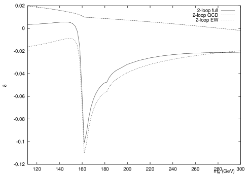
(a)	(b)

Figure 4: (a) $\mathcal{O}(G_{F}M_{t}^{2})$ fugel (solid line), $\mathcal{O}(\alpha_{s})$ Djouadi:1990aj (dashed line), and (b) $\mathcal{O}(n_{f}G_{F}M_{W}^{2})$ Aglietti:2004nj (dotted line) two-loop corrections to $\Gamma(H\to\gamma\gamma)$ as functions of $M_{H}$.

For the comparison with future measurements of $\Gamma(H\to\gamma\gamma)$, all known corrections have to be included in Eq. (3). In this connection, it is interesting to compare the $\mathcal{O}(G_{F}M_{t}^{2})$ electroweak correction discussed above with the well-known $\mathcal{O}(\alpha_{s})$ QCD correction Djouadi:1990aj and the $\mathcal{O}(N_{f}G_{F}M_{W}^{2})$ electroweak correction induced by light-fermion loops, which has become available recently Aglietti:2004nj . This is done in Figs. 4(a) and (b), where the respective corrections to $\Gamma(H\to\gamma\gamma)$ are displayed as functions of $M_{H}$. As in Fig. 3, the dotted vertical line and the right edge of the frame in Fig. 4(a) margin the $M_{H}$ range $M_{W}\leq M_{H}\leq 2M_{W}$. We observe that, within the latter, the $\mathcal{O}(G_{F}M_{t}^{2})$ correction slightly exceeds the $\mathcal{O}(\alpha_{s})$ one in magnitude, a rather surprising finding. Due to the sign difference, the two corrections practically compensate each other. The $\mathcal{O}(N_{f}G_{F}M_{W}^{2})$ correction is also negative, but has a slightly smaller size than the $\mathcal{O}(G_{F}M_{t}^{2})$ one.

V Conclusions

We discussed the dominant two-loop electroweak correction, of $\mathcal{O}(G_{F}M_{t}^{2})$, to the partial width of the decay into two photons of the SM Higgs boson in the intermediate mass range, $M_{W}\leq M_{H}\leq 2M_{W}$, where this process is of great phenomenological relevance for searches at hadron colliders and precision tests at the ILC.

The relevant Feynman diagrams were evaluated with the aid of the asymptotic-expansion technique exploiting the mass hierarchy $M_{H}\ll 2M_{W}\ll 2M_{t}$. In this way, an expansion of the full $\mathcal{O}(G_{F}M_{t}^{2})$ result in the mass ratio $\tau_{W}=M_{H}^{2}/(2M_{W})^{2}$ through $\mathcal{O}(\tau_{W}^{4})$ was obtained. The convergence property of this expansion and the experience with the analogue expansion at the Born level, where the exact result is available for reference, lead one to believe that these five terms should provide a very good approximation to the exact result for $M_{H}\lesssim 140$ GeV. By the same token, the deviation of this approximation for the $\mathcal{O}(G_{F}M_{t}^{2})$ amplitude $\mathcal{A}_{tW}^{(1)}$ from the unknown exact result for this quantity is likely to range from 2% to 20% as the value of $M_{H}$ runs from 140 GeV to $2M_{W}$.

In the intermediate Higgs-boson mass range, the $\mathcal{O}(G_{F}M_{t}^{2})$ electroweak correction reduces the size of $\Gamma(H\to\gamma\gamma)$ by approximately 2.5% and thus fully cancels the positive shift due to the well-known $\mathcal{O}(\alpha_{s})$ QCD correction Djouadi:1990aj .

As a by-product of this analysis, also the $\mathcal{O}(G_{F}M_{t}^{2})$ correction to the partial width of the decay into two gluon jets of the intermediate-mass Higgs boson was recovered Djouadi:1994ge .

Note added

After the workshop, a preprint Degrassi:2005mc appeared in which the two-loop electroweak corrections to $\Gamma(H\to\gamma\gamma)$ involving intermediate bosons and the top quark are computed as expansions in $q^{2}/(2M_{W})^{2}$, where $q$ is the four-momentum of the decaying Higgs boson. In that paper, also the key result of Ref. fugel , Eq. (8), is confirmed.

- (1) The LEP Collaborations ALEPH, DELPHI, L3, OPAL, the LEP Electroweak Working Group, the SLD Electroweak and Heavy Flavour Groups, D. Abbaneo et al., Report No. CERN-PH-EP/2004-069 and hep-ex/0412015.
- (2) T. Hambye and K. Riesselmann, Phys. Rev. D 55 (1997) 7255.
- (3) B.A. Kniehl, Phys. Rept. 240 (1994) 211.
- (4) J.R. Ellis, M.K. Gaillard, and D.V. Nanopoulos, Nucl. Phys. B 106 (1976) 292.
- (5) H. Zheng and D. Wu, Phys. Rev. D 42 (1990) 3760.
- (6) M. Steinhauser, in: B.A. Kniehl (Ed.), Proceedings of the Ringberg Workshop on the Higgs Puzzle — What can we learn from LEP2, LHC, NLC, and FMC?, Ringberg Castle, Germany, 8–13 December 1996, World Scientific, Singapore, 1997, p. 177, Report No. hep-ph/9612395.
- (7) J.G. Körner, K. Melnikov, and O.I. Yakovlev, Phys. Rev. D 53 (1996) 3737.
- (8) A. Djouadi, P. Gambino, and B.A. Kniehl, Nucl. Phys. B 523 (1998) 17.
- (9) B.A. Kniehl and M. Spira, Z. Phys. C 69 (1995) 77; W. Kilian, Z. Phys. C 69 (1995) 89; K.G. Chetyrkin, B.A. Kniehl, and M. Steinhauser, Nucl. Phys. B 510 (1998) 61.
- (10) U. Aglietti, R. Bonciani, G. Degrassi, and A. Vicini, Phys. Lett. B 595 (2004) 432.
- (11) F. Fugel, B.A. Kniehl, and M. Steinhauser, Nucl. Phys. B 702 (2004) 333.
- (12) Particle Data Group, K. Hagiwara et al., Phys. Rev. D 66 (2002) 010001.
- (13) V.A. Smirnov, Applied Asymptotic Expansions in Momenta and Masses, Springer-Verlag, Berlin-Heidelberg, 2001.
- (14) A. Djouadi and P. Gambino, Phys. Rev. Lett. 73 (1994) 2528; K.G. Chetyrkin, B.A. Kniehl, and M. Steinhauser, Phys. Rev. Lett. 78 (1997) 594; Nucl. Phys. B 490 (1997) 19.
- (15) B.A. Kniehl and A. Sirlin, Phys. Lett. B 318 (1993) 367; B.A. Kniehl, Phys. Rev. D 50 (1994) 3314.
- (16) G. Degrassi and F. Maltoni, Report No. RM3-TH/05-03, CERN-PH-TH/2005-064, and hep-ph/0504137.