Light Mesons and Muon Radiative Decays and Photon Polarization Asymmetry

Emidio Gabrielli^a and Luca Trentadue^b

^aHelsinki Institute of Physics, P.O.B. 64, 00014 University of Helsinki, Finland
^bDipartimento di Fisica, Universitá di Parma,
and
INFN, Gruppo Collegato di Parma, Viale delle Scienze 7, 43100 Parma, Italy

We systematically compute and discuss meson and muon polarized radiative decays. Doubly differential distributions in terms of momenta and helicities of the final lepton and photon are explicitly computed. The undergoing dynamics giving rise to lepton and photon polarizations is examined and analyzed in the soft and hard region of momenta. The particular configurations made by right-handed leptons with accompanying photons are investigated and interpreted as a manifestation of the axial anomaly. The photon polarization asymmetry is evaluated. Finiteness of polarized amplitudes against infrared and collinear singularities is shown to take place with mechanisms distinguishing between right handed and left handed final leptons. We propose a possible test using photon polarization to clarify a recently observed discrepancy in radiative meson decays.

1 Introduction

Radiative decays of light mesons and leptons have been widely studied both experimentally and theoretically. They represent an excellent source of information on the experimental side as well as a benchmark for theoretical speculations. Extensive comparisons have been carried on in the past between experiments and theoretical predictions for meson radiative decays (see for example Ref.[1]). A while ago, radiative polarized leptonic decays of mesons [2, 3] and muons [4, 5] have also been considered. Recently special attention has been given to the role played by the final lepton mass $m_{l}$ in the threshold region of the decay and to the $m_{l}\rightarrow 0$ limit concerning the helicity amplitudes for mesons [3] and leptons Refs.[4, 5]. The $O(\alpha)$ radiative corrections generate an helicity flip of the final lepton even in the zero mass limit [6] provided the lepton mass is kept from the beginning into account. Following the interpretation due to Dolgov and Zakharov [7] of the axial anomaly the final states with opposite helicity can be interpreted [9, 8, 3], as a manifestation of the axial anomaly giving rise to a peculiar mass-singularity cancellation for the right-handed polarized final lepton amplitudes.

We consider in this work the case of polarized radiative decays of the pion and kaon meson and of the muon more extensively by taking into account polarizations of final lepton and photon degrees of freedom. Contrary to the previous case [2], in meson decays we consider the polarization states of both lepton and photon final states.

This approach, containing a complete description of the final momenta and helicities, may give further and more detailed information on the final state with respect to the inclusively polarized and unpolarized cases. Furthermore, the agreement with the more inclusive results previously obtained in the literature can be easily recovered by summing over the emitted final states polarizations. It is worth noticing that this approach allows to describe more closely the interplay between several peculiar features of the dynamics involved. As, for instance, to pinpoint the role played by angular momentum conservation and its connection with hard and soft photon momenta, and to consider the role played by the parity conservation in weak decays. All these aspects related to angular momentum dynamics may be effectively described in terms of the photon polarization asymmetry.

Here we emphasize that the knowledge of the helicity amplitudes of the final leptons and photons, in addition to an explicit test of the angular momentum conservation, shows the relative rates of the partial helicity amplitudes. Indeed, in the total rate, different helicity amplitudes, depending on the range of momenta, enter with varying weights. Therefore, this behavior gives the opportunity to isolate peculiar polarized configurations in order to maximize or minimize them according to favorable intervals of momenta. As far as phenomenological applications are concerned, this may be, as will be discussed later, an effective way to compare theory and experiment on a new basis. The case of the photon polarization asymmetry, proposed in this work, allows, in this respect, a new approach to inspect interaction dynamics via a finite and universal quantity which is also directly associated to parity violation. Moreover, the photon polarization asymmetry is very sensitive, in radiative meson decays, to the hadronic structure, allowing for a more precise determination of the electromagnetic form factors with respect to the one obtained so far.

Some of the results achieved in this paper can be shortly listed: we explicitly calculate amplitudes and final distributions in terms of lepton and photon momenta at fixed final lepton and photon helicities. Double differential expressions in terms of lepton and photon momenta are also provided together with the partial helicity amplitudes for the meson and muon cases respectively. Moreover, we analyze how the cancellation pattern of mass singularities works on polarized processes. In the inclusive quantities this is a sensible test of the consistency of the results. Once inclusive distributions are obtained by integrating over final momenta, we observe the cancellation of all mass singularities both infrared and collinear. In particular, a peculiar pattern of mass singularity cancellation is shown to take place, which differs for the left-handed helicity final lepton states with respect to the right-handed ones. The same behavior can be observed for the meson as well as for the muon case.

Finally, we discuss a possible interpretation in terms of tensorial coupling of the results obtained recently at the PIBETA experiment [10] for the radiative pion decay in electron channel. It is argued that polarized radiative processes may constitute a sensible test to resolve the controversial issue of tensorial couplings in radiative pion decay, allowing also for a sensitive test in the corresponding kaon decays as well.

The paper is organized as follows: In Section 2 we consider the case of the meson polarized radiative decay. We discuss the contributing amplitudes and the underlying theoretical tools. We also define the gauge invariant set of matrix elements together with the definition of the Lorentz invariant quantities. Allowed and forbidden helicities configurations are here analyzed as well. In Section 3 the polarized radiative muon decay is discussed. In Section 4 we define distributions of branching ratios in the photon and electron energies and the photon polarization asymmetry. Numerical results for the distributions of branching ratios and polarization asymmetries are provided in subsections 4.1, 4.2, and 4.3 for the cases of pion, kaon, and muon decays respectively. Results for the polarized electron energy spectra are presented in Section 5. In Section 6 the dependence of the photon polarization asymmetry, induced by tensorial couplings, is discussed in the radiative pion and kaon decays. The peculiar pattern of mass singularities cancellation in polarized radiative decays is described in Section 7, while conclusions are presented in Section 8. General results and the corresponding formulae for the polarized radiative meson and muon decays are collected in Appendix A and B respectively.

2 The polarized radiative meson decay

We start this section with the calculation of the polarized amplitude for the process

$$M^{+}(p)\to\nu_{l}(p_{\nu})~{}l^{+}(p_{l},\lambda_{l})~{}\gamma(k,\lambda_{\gamma})\,,$$ (1)

where $M^{+}=\pi^{+}~{}(K^{+})$ and $l=e~{}(\mu)$ stand for pion (kaon) and electron (muon) respectively, with $\nu_{l=e,\mu}$ the corresponding neutrinos. The four momenta $p,p_{\nu},p_{l}$ correspond to meson $M$, neutrino, and charged lepton, while $\lambda_{l},\lambda_{\gamma}$ indicate the charged lepton and photon helicity, respectively. The neutrino is assumed massless and therefore is a pure left-handed polarized state. The Feynman diagrams at tree-level for this process are shown in Fig.1, where the green bubble just indicates the Fermi interaction.

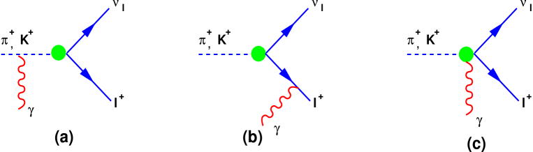
Figure 1: Feynman diagrams for $(\pi^{+},K^{+})\to\nu_{l}l^{+}\gamma$ decay, where $l=e,\mu$

The first two diagrams Figs.1a-b correspond to the so-called inner bremsstrahlung (IB) diagrams, where the photon is emitted from external lines and the meson behaves as a point-like scalar particle. The third diagram Fig.1c is the so-called structure-dependent (SD) diagram, where the photon is emitted from an intermediate hadronic state and the matrix element will depend on the vectorial (V) and axial (A) meson form factors. The total amplitude for this process can be split in two gauge invariant contributions

$${\rm M}^{(\lambda_{l},\lambda_{\gamma})}={\rm M}_{IB}^{(\lambda_{l},\lambda_{\gamma})}+{\rm M}_{SD}^{(\lambda_{l},\lambda_{\gamma})}\,,$$ (2)

where ${\rm M}_{IB}$ and ${\rm M}_{SD}$ correspond to the IB and SD part of the amplitude. The IB amplitude is given by [11, 12]

$${\rm M}_{IB}^{(\lambda_{l},\lambda_{\gamma})}=\frac{ieG_{F}}{\sqrt{2}}m_{l}f_{M}V_{uq}~{}\epsilon^{\star}_{\mu}(k,\lambda_{\gamma})\left[\bar{u}(p_{\nu})\left(\frac{p^{\mu}}{\left(p\cdot k\right)}-\frac{/k\gamma^{\mu}+2p^{\mu}_{l}}{2\left(p_{l}\cdot k\right)}\right)\left(1+\gamma_{5}\right)v(p_{l},\lambda_{l})\right]\,,$$ (3)

where $/k=\gamma^{\alpha}k_{\alpha}$, $\epsilon_{\mu}(k,\lambda_{\gamma})$ stands for the photon polarization vector of momentum $k$ and helicity $\lambda_{\gamma}$, while $\bar{u}(p_{\nu})$ and $v(p_{l},\lambda_{l})$ are the bispinors of final neutrino and charged lepton respectively. Explanations of other symbols appearing above are in order. The $G_{F}$ is the Fermi constant, $m_{l}$ is the charged lepton mass, $f_{M}$ is the meson decay constant, where $f_{\pi}\simeq 131$ MeV and $f_{K}\simeq 161$ MeV, and $V_{uq}$ is the Cabibbo-Kobayashi-Maskawa matrix element corresponding to $u\to q=d$ and $u\to q=s$ quark transitions for pion and kaon decays respectively.

The SD part of the amplitude contains vectorial $(V)$ and axial $(A)$ form factors, that clearly depend on the kind of initial meson, but not on the lepton final states. Indeed, they are connected to the matrix elements of the electromagnetic hadron current $V_{\rm em}^{\mu}$ and the axial and vectorial weak currents $A^{\mu}$ and $V^{\mu}$ respectively, as

$$({\rm V,A})^{\mu\nu}(p,k)\equiv\int d^{4}xe^{ikx}\langle 0|~{}TV^{\mu}_{\rm em}(x)(V(0),A(0))^{\nu}~{}|M^{+}(p)\rangle\,.$$ (4)

Using Lorentz covariance and electromagnetic gauge invariance, it follows that:

$${\rm V}^{\mu\nu}(p,k) = i\frac{V}{m_{M}}\epsilon^{\mu\nu\alpha\beta}k_{\alpha}p_{\beta}$$

$${\rm A}^{\mu\nu}(p,k) = (p\cdot k)\frac{A}{m_{M}}\left(\eta^{\mu\nu}-\frac{p^{\mu}k^{\nu}}{(p\cdot k)}\right)-f_{M}\left(\eta^{\mu\nu}+\frac{p^{\mu}\left(p^{\nu}-k^{\nu}\right)}{(p\cdot k)}\right)\,,$$ (5)

where $\eta^{\mu\nu}={\rm diag}(1,-1,-1,-1)$ is the Minkowski metric, and $\epsilon^{\mu\nu\alpha\beta}$ is the totally antisymmetric tensor . Finally, the SD part of the amplitude is given by [11, 12]

$${\rm M}_{SD}^{(\lambda_{l},\lambda_{\gamma})} = -\frac{ieG_{F}}{\sqrt{2}}V_{uq}~{}\epsilon^{\star}_{\mu}(k,\lambda_{\gamma})\left\{\left(p\cdot k\right)\frac{A}{m_{M}}\left(-\eta^{\mu\nu}+\frac{p^{\mu}k^{\nu}}{\left(p\cdot k\right)}\right)+i\epsilon^{\mu\nu\alpha\beta}\frac{V}{m_{M}}k_{\alpha}p_{\beta}\right\}$$ (6)

$$\times \Big{[}\bar{u}(p_{\nu})\gamma_{\nu}\left(1-\gamma_{5}\right)v(p_{l},\lambda_{l})\Big{]}\,,$$

where $m_{M}$ stands for the meson mass, while $V$ and $A$ are the meson vectorial and axial form factors respectively. Notice that both the terms $M_{IB}$ and $M_{SD}$ are separately gauge invariant, as can be easily checked by making the substitution $\epsilon^{\star}_{\mu}(k,\lambda_{\gamma})\to\epsilon^{\star}_{\mu}(k,\lambda_{\gamma})+k_{\mu}$ in Eqs.(3) and (6).

Now we provide the corresponding expressions for the polarized amplitude in the center of mass (c.m.) frame of the fermion pair (neutrino and charged lepton), namely $\vec{p}_{l}+\vec{p}_{\nu}=0$. We choose a frame where the 3-momenta of neutrino and photon have the following components in polar coordinates

$$\vec{p}_{\nu}=E_{\nu}~{}\left(\sin{\theta}\cos{\varphi},\sin{\theta}\sin{\varphi},\cos{\theta}\right),~{}~{}~{}\vec{p}_{l}=-\vec{p}_{\nu},~{}~{}~{}~{}\vec{k}=E_{\gamma}~{}(0,0,1)\,,$$ (7)

where $E_{\nu}$ and $E_{\gamma}$ are the neutrino and photon energies respectively and $\theta,\varphi$ are the usual polar angles. For the photon polarization vectors we choose helicity eigenstates ($\epsilon(k,\lambda)$), which in this frame are given by

$$\epsilon_{\mu}(k,\lambda_{\gamma})=\frac{1}{\sqrt{2}}\left(0,1,i\lambda_{\gamma},0\right)$$ (8)

whose helicity eigenvalues correspond to $\lambda_{\gamma}=-1$ left-handed (L) and $\lambda_{\gamma}=1$ right-handed (R) circular polarizations. Photon polarization vectors satisfy the transversality condition $k^{\mu}\epsilon_{\mu}(k,\lambda_{\gamma})=0$. Regarding the polarization vectors of fermions, it is convenient to use the solution of the Dirac equation for the particle ($u$) and antiparticle ($v$) bispinors in the momentum space [13]. In the standard basis we have:

$$u(p,\lambda)=\left(\begin{array}[]{c}\sqrt{E+m}\,\,\omega_{\lambda}(\vec{n})\\ \sqrt{E-m}\,\,\left(\vec{\sigma}\cdot\vec{n}\right)\omega_{\lambda}(\vec{n})\end{array}\right)~{}~{}~{}~{}~{}v(p,-\lambda)=\left(\begin{array}[]{c}\sqrt{E-m}\,\,\left(\vec{\sigma}\cdot\vec{n}\right)\omega_{\lambda}(\vec{n})\\ \sqrt{E+m}\,\,\omega_{\lambda}(\vec{n})\end{array}\right)\,,$$ (13)

where the 2-component spinors $\omega_{\lambda}(\vec{n})$ (with helicity $\lambda=\pm 1$) are the eigenstates of the helicity operator $\left(\vec{\sigma}\cdot\vec{n}\right)\omega_{\lambda}(\vec{n})=\lambda\,\omega_{\lambda}(\vec{n})$, and $\;\sigma_{i}$ are the Pauli matrices. Here, $\vec{n}\equiv\vec{p}/|\vec{p}|$, where $\vec{p}$ is the 3-momentum and $E=\sqrt{|\vec{p}|^{2}+m^{2}}$ is the corresponding energy. If $\vec{p}=|\vec{p}|\left(\sin{\theta}\cos{\varphi},\sin{\theta}\sin{\varphi},\cos{\theta}\right)$, then in polar coordinates, $\omega_{\lambda}(\vec{n})$ can be expressed as

$$\omega_{+1}(\vec{n})=\left(\begin{array}[]{c}e^{-i\frac{\varphi}{2}}\,\cos{\frac{\theta}{2}}\\ e^{i\frac{\varphi}{2}}\,\sin{\frac{\theta}{2}}\end{array}\right)\,,~{}~{}~{}~{}~{}\omega_{-1}(\vec{n})=\left(\begin{array}[]{c}-e^{-i\frac{\varphi}{2}}\,\sin{\frac{\theta}{2}}\\ e^{i\frac{\varphi}{2}}\,\cos{\frac{\theta}{2}}\end{array}\right)\,.$$ (18)

At this point it is convenient to introduce the following Lorentz invariant quantities

$$x\equiv\frac{2p\cdot k}{m_{M}^{2}},~{}~{}~{}~{}y\equiv\frac{2p\cdot p_{l}}{m_{M}^{2}},~{}~{}~{}~{}z\equiv\frac{2p_{l}\cdot k}{m_{M}^{2}}=y-1+x-r_{l}$$ (19)

where in the meson rest frame, $x$ and $y$ are just proportional to the photon and charged lepton energies respectively and $r_{l}=m_{l}^{2}/m_{M}^{2}$. Finally, after a straightforward algebra, the $IB$ and $SD$ contributions to the polarized amplitude in the fermion pair c.m. frame are given by

$${\rm M}_{IB}^{(\lambda_{l},\lambda_{\gamma})} = eG_{F}m_{l}f_{M}V_{uq}~{}\frac{2}{z}\left\{\delta_{\lambda_{l},-1}\left(\delta_{\lambda_{\gamma},-1}~{}\hat{E}_{\gamma}+\hat{E}_{\nu}\right)R_{+}\sin{\theta}\right.$$

$$+ \left.\delta_{\lambda_{l},+1}~{}\delta_{\lambda_{\gamma},-1}~{}\hat{E}_{\gamma}R_{-}\left(1-\cos{\theta}\right)\right\}e^{i\lambda_{\gamma}\varphi}$$

$${\rm M}_{SD^{\pm}}^{(\lambda_{l},\lambda_{\gamma})} = eG_{F}m_{M}^{2}V_{uq}~{}\frac{\left(V\pm A\right)}{2}~{}\delta_{\lambda_{\gamma},\pm 1}~{}x\Big{\{}\mp\delta_{\lambda_{l},-1}~{}R_{-}\sin{\theta}$$ (20)

$$\pm \delta_{\lambda_{l},+1}R_{+}\left(\cos{\theta}\pm 1\right)\Big{\}}~{}e^{i\lambda_{\gamma}\varphi}\,,$$

where the structure dependent part is given by ${\rm M}_{SD}^{(\lambda_{l},\lambda_{\gamma})}={\rm M}_{SD^{+}}^{(\lambda_{l},\lambda_{\gamma})}+{\rm M}_{SD^{-}}^{(\lambda_{l},\lambda_{\gamma})}$ and the symbol $R_{\pm}\equiv\sqrt{\hat{E}_{\nu}}\left(\sqrt{\hat{E}_{l}+\sqrt{r_{l}}}\pm\sqrt{\hat{E}_{l}-\sqrt{r_{l}}}\right)$, with $\hat{E}_{i}\equiv E_{i}/m_{M}$ and $E_{l}$ is the energy of the final charged lepton. In this frame, the energies normalized to the meson mass are given by

$$\hat{E}_{\gamma} = \frac{x}{2\sqrt{1-x}},~{}~{}~{}~{}\hat{E}_{\nu}=\frac{1-x-r_{l}}{2\sqrt{1-x}},~{}~{}~{}\hat{E}_{l}=\frac{1-x+r_{l}}{2\sqrt{1-x}},$$

$$\cos{\theta} = \frac{(x-2)(1-x+r_{l})+2y(1-x)}{x(1-r_{l}-x)}$$ (21)

and

$$R_{+} = \sqrt{1-r_{l}-x},~{}~{}~{}R_{-}=\sqrt{r_{l}\frac{1-r_{l}-x}{1-x}}\,.$$ (22)

Notice that, as expected from general arguments, the azimuthal angle $\varphi$ factorizes in the overall phase of the amplitude. At this point it is important to stress that the SD terms in the amplitude, proportional to $V+A$ and $V-A$, correspond to pure right-handed and left-handed photon polarizations respectively, while the IB one is a mixture of both. In particular, the terms proportional to pure left-handed photon polarizations in the $M_{IB}$, come only from the tensorial structure in Eq.(3), namely from terms proportional to $[\bar{u}_{\nu}~{}\sigma_{\mu\nu}(1+\gamma_{5})~{}v_{l}]$, while scalar contributions of type $[\bar{u}_{\nu}~{}(1+\gamma_{5})~{}v_{l}]$ do not select any specific photon polarization. We will return on this point in the following when anomalous tensorial coupling in radiative pion, and kaon decays will be discussed.

By using Eqs.(20) and (21), it is now straightforward to evaluate the square modulus of the amplitude. Below we will provide its expression summed over the charged lepton polarizations, as a function of the photon helicities. After integrating over the phase space, we obtain for the photon polarized decay rate $\Gamma^{\lambda_{\gamma}}$, the following result:

$$\frac{d^{2}\Gamma^{(\lambda_{\gamma})}}{dx~{}d\lambda}=\frac{m_{\rm M}}{256\pi^{3}}\sum_{\lambda_{l}=\pm 1}|{\rm M}^{(\lambda_{l},\lambda_{\gamma})}|^{2}=\rho^{(\lambda_{\gamma})}(x,\lambda)\,.$$ (23)

Here $m_{\rm M}$ stands for the generic meson mass $m_{{\rm M}=\pi,K}$, and $\lambda\equiv z/x$. The Dalitz plot densities $\rho^{\lambda_{\gamma}}(x,\lambda)$ for the polarized decay are Lorentz invariant functions, and are given by

$$\rho^{(-1)}(x,\lambda) = A_{\scriptscriptstyle IB}~{}f_{\scriptscriptstyle IB}^{\rm L}(x,\lambda)+A_{\scriptscriptstyle SD}~{}\frac{1}{2}(V-A)^{2}f_{\scriptscriptstyle SD}^{\rm L}(x,\lambda)+A_{\scriptscriptstyle INT}(V-A)f_{\scriptscriptstyle INT}^{\rm L}(x,\lambda)~{}~{}~{}$$ (24)

$$\rho^{(+1)}(x,\lambda) = A_{\scriptscriptstyle IB}~{}f_{\scriptscriptstyle IB}^{\rm R}(x,\lambda)+A_{\scriptscriptstyle SD}~{}\frac{1}{2}(V+A)^{2}f_{\scriptscriptstyle SD}^{\rm R}(x,\lambda)+A_{\scriptscriptstyle INT}(V+A)f_{\scriptscriptstyle INT}^{\rm R}(x,\lambda)\,,~{}~{}~{}$$ (25)

where

$$A_{\scriptscriptstyle IB} = 2\,r_{l}\left(\frac{f_{M}}{m_{M}}\right)^{2}A_{\scriptscriptstyle SD},~{}~{}~{}A_{\scriptscriptstyle INT}=2\,r_{l}\,\frac{f_{M}}{m_{M}}\,A_{\scriptscriptstyle SD}$$

$$A_{\scriptscriptstyle SD} = \frac{\alpha}{32\pi^{2}}\,G_{F}^{2}\,m_{M}^{5}\,|V_{uq}|^{2}\,.$$ (26)

In the following, for later convenience, we will introduce the labels R and L corresponding to photon helicities $\lambda_{\gamma}=1$ and $\lambda_{\gamma}=-1$ respectively. The functions $f^{\rm L,R}_{\scriptscriptstyle IB}(x,\lambda),~{}f_{\scriptscriptstyle SD}^{L,R}(x,\lambda)$, and $f_{\scriptscriptstyle INT}^{L,R}(x,\lambda)$ are given by

$$f^{\rm L}_{\scriptscriptstyle IB}(x,\lambda) = \frac{1-\lambda}{x\lambda}\left(1+r_{l}\left(x-1\right)-\frac{r_{l}}{\lambda}\left(1+x-r_{l}\right)\right)$$

$$f^{\rm R}_{\scriptscriptstyle IB}(x,\lambda) = \frac{1-\lambda}{x\lambda}\left(x-1+\frac{r_{l}}{\lambda}\right)\left(x-1+r_{l}\right)$$

$$f_{\scriptscriptstyle SD}^{\rm R}(x,\lambda) = x^{2}\lambda\left(\left(1-x\right)\left(x\lambda+r_{l}\right)-r_{l}\right)$$

$$f_{\scriptscriptstyle SD}^{\rm L}(x,\lambda) = x^{2}\left(1-\lambda\right)\left(\left(x-1\right)\left(r_{l}+x\left(\lambda-1\right)\right)+r_{l}\right)$$

$$f_{\scriptscriptstyle INT}^{\rm R}(x,\lambda) = \frac{1-\lambda}{\lambda}\left(\left(x-1\right)\left(x\lambda+r_{l}\right)+r_{l}\right)$$

$$f_{\scriptscriptstyle INT}^{\rm L}(x,\lambda) = \frac{1-\lambda}{\lambda}\left(x^{2}+\left(1-x\right)\left(x\lambda+r_{l}\right)-r_{l}\right)\,.$$ (27)

The function $f^{\rm L}_{\scriptscriptstyle IB}(x,\lambda)+f^{\rm R}_{\scriptscriptstyle IB}(x,\lambda)$ coincides with the corresponding IB function $f_{\scriptscriptstyle IB}(x,\lambda)$ for the unpolarized case provided in [14, 11, 12], as well as $f_{\scriptscriptstyle SD}(x,\lambda)=f_{\scriptscriptstyle SD}^{L}(x,\lambda)+f_{\scriptscriptstyle SD}^{R}(x,\lambda)$ and $f_{\scriptscriptstyle INT}(x,\lambda)=f_{\scriptscriptstyle INT}^{L}(x,\lambda)+f_{\scriptscriptstyle INT}^{R}(x,\lambda)$. More general results for the complete polarized radiative decay rate, including also the charged lepton helicity in the pion rest frame, are provided in appendix A.

In order to obtain the differential branching ratio (${\rm BR}$) it is convenient to rewrite the term $A_{SD}$ in Eq.(26) as

$$A_{\scriptscriptstyle SD}=\frac{\alpha}{4\pi}\frac{1}{r_{l}\left(1-r_{l}\right)^{2}}\left(\frac{m_{M}}{f_{M}}\right)^{2}\Gamma_{0}$$ (28)

where $\Gamma_{0}=\Gamma(M\to l\nu_{l})$ is Born contribution to the total width of non radiative decay $M\to l\nu_{l}$, in particular

$$\Gamma_{0}(M^{+}(p)\to\nu_{l}+l^{+})=\frac{G_{F}^{2}\,f_{M}^{2}\,m_{M}}{8\pi}|V_{uq}]^{2}r_{l}\,(1-r_{l})^{2}\,.$$ (29)

Then

$$\frac{d^{2}{\rm BR}}{{dx~{}d\lambda}}={\rm BR}(M\to l\nu_{l})~{}\frac{1}{\Gamma_{0}}\frac{d^{2}\Gamma}{dx~{}d\lambda}\,,$$ (30)

where ${\rm BR}(M\to l\nu_{l})$ is the total branching ratio of the corresponding non radiative decay. Finally, the total branching ratio ${\rm BR}$ is obtained by integrating Eq.(30) in the full kinematical range as follows

$${\rm BR}=\int dx\int d\lambda~{}\frac{d^{2}{\rm BR}}{{dx~{}d\lambda}}$$ (31)

$$0\leq x\leq 1-r_{l},~{}~{}~{}~{}~{}\frac{r_{l}}{1-x}\leq\lambda\leq 1\,.$$ (32)

In case in which kinematical cuts ($x^{\rm min}$, and $\lambda^{\rm min}$) should be applied, the minima of integrations should be replaced as

$$x^{\rm min}\leq x\leq 1-r_{l},~{}~{}~{}~{}~{}{\rm max}\left\{\lambda^{\rm min},~{}\frac{r_{l}}{1-x}\right\}\leq\lambda\leq 1\,.$$ (33)

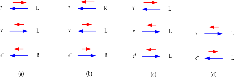
Figure 2: Allowed helicity (in red) configurations of $\gamma$, $\nu$ and $e^{+}$ for $\pi^{+}\to e^{+}\nu_{e}\gamma$ decay in $\pi^{+}$ rest frame, figures (a),  (b),  (c), when all momenta (in blue) are aligned on the same axis. Direction of photon momentum is fixed by convention. Figure (d) corresponds to the non radiative decay $\pi^{+}\to e^{+}\nu_{e}$. Analogous spin configurations hold for the corresponding $K^{+}$ decays as well.

Let us now consider the positron decay mode, where, as a good approximation, the lepton mass can be neglected in comparison to the pion one. A remarkable aspect of the results in Eq.(27), is that in the limit in which $\lambda\to 0$ and $x\to 1$, which corresponds to the emission of low energy positron and hard photons at relative small angles in the meson rest frame, the contribution proportional to $f_{\scriptscriptstyle IB}^{\rm L}(x,\lambda)$ and to $f_{\scriptscriptstyle INT}^{\rm L}(x,\lambda)$ distributions dominates in the decay rate. In other words, hard photons will be mainly produced with left-handed polarizations. This behavior, as will be shown in more details in section 4, is just a consequence of the V-A nature of weak interactions and of the angular momentum conservation. This can be easily understood as follows. In the $\pi^{+}$ rest frame, neglecting the lepton mass, we have $x=2E_{\gamma}/m_{M}$, and $\lambda=E_{e}/m_{M}(1-\cos{\theta_{\gamma e}})$, where $\theta_{\gamma e}$ is the angle between positron and photon momenta. Let us consider the kinematical region in which $\lambda\to 0$, which corresponds to $E_{e}\to 0$ and/or $\theta_{\gamma e}\to 0$. Due to the conservation of total momentum, and to the fact that $|\vec{p}_{e}|/m_{M}\ll 1$ and $\theta_{\gamma e}\to 0$, the neutrino must be emitted in this region almost backward with respect to the photon direction, therefore final momenta are almost aligned on the same axis. This configuration is shown in Fig.2a, where all momenta are chosen to be aligned on the same axis. One then could easily check the conservation of the spin $(S_{X})$ along the direction of the photon momentum which in Fig.2 is set by convention on the negative $X$-axis. Since neutrino is a purely left-handed state, its spin projection along $X$-axis would be $S_{X}(\nu_{l})=+1/2$. As a consequence of the angular momentum conservation ($S_{X}(\pi)=0$ for pion), the photon must also be left-handed polarized giving $S_{X}(\gamma)=-1$. In this case the positron, whose momentum is parallel to the one of the photon, must be right-handed in order to satisfy the total sum $S_{X}(\gamma)+S_{X}(\nu_{e})+S_{X}(e^{+})=0$. Notice that, in this particular kinematical limit $\lambda\to 0$, photons with right-handed polarization would be suppressed, since the total sum of spins along $X$-axis would give in that case $S_{X}(\gamma)+S_{X}(\nu_{l})=3/2$ thus spoiling angular momentum conservation. It is worth noticing that also in the case of $\pi^{+}\to\mu^{+}\nu\gamma$ decay mode, where the muon mass cannot be neglected in comparison to the one of the pion, the left-handed photon amplitude still dominates for high energy photons. This fact can be explained as follows. When the photon energy approaches its maximum value, being neutrino massless, in order to conserve total momentum, the production of the $\mu^{+}$ at rest it is favored. In this case the momentum of the neutrino should be opposite to one of the photon. As explained above, for this kinematical configuration, the photon is therefore favored to be produced as left-handed in order to conserve total angular momentum. Same considerations apply to the corresponding kaon decays as well.

Another interesting case is the one in which the photon energy tends to zero, namely $x\to 0$. In this singular kinematical region, one should expect soft photons to behave as scalar particles, carrying no spin. Then in this limit both the left-handed or right-handed distributions should tend to the same value, as indeed can be verified by performing the limit $x\to 0$ on the density distributions in Eq.(27). In the following we will show how this property could be relevant in order to define an observable which is free from infrared ($E_{\gamma}\to 0$) singularity, namely the photon polarization asymmetry.

3 The polarized radiative muon decay

Here we analyze the radiative muon decay

$$\mu^{-}(p)\to\nu_{\mu}(q_{1})\,\bar{\nu}_{e}(q_{2})\,e^{-}(p_{e})\,\gamma(k)$$ (34)

in which both photon and electron final states are polarized. The corresponding Feynman diagrams for this process are shown in Fig.3, where $p,\,p_{e},\,q_{1,2},\,k$ are the corresponding momenta.

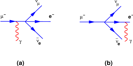
Figure 3: Feynman diagrams for $\mu^{-}\to\nu_{\mu}\bar{\nu}_{e}e^{-}\gamma$ decay.

This decay is obtained from the non radiative one $\mu^{-}\to\nu_{\mu}\,\bar{\nu}_{e}\,e^{-}$, by simply attaching the photon to the muon and electron external lines. Due to the V-A nature of weak interactions and a simple Fierz rearrangement, the square modulus of the polarized amplitude can be factorized as follows [4, 5, 15]

$$|M^{(\lambda_{\gamma},\lambda_{e})}|^{2}=\frac{G_{F}^{2}}{2}\,\Big{[}M_{\alpha}^{(\lambda_{\gamma},\lambda_{e}){\dagger}}\,M_{\beta}^{(\lambda_{\gamma},\lambda_{e})}\Big{]}\,\Big{[}N^{\alpha{\dagger}}\,N^{\beta}\Big{]}\,,$$ (35)

where $M^{\alpha}(\lambda_{e},\lambda_{\gamma})$ corresponds to the ${\cal O}(\alpha)$ amplitude in which photon is either radiated off the electron or off the muon, and $N^{\alpha}$ to the neutrino amplitude respectively

$$M^{\alpha}(\lambda_{\gamma},\lambda_{e}) = e\,\bar{u}_{e}(p_{e},\lambda_{e})\left(\gamma^{\delta}\frac{\ooalign{\hfil/\hfil\crcr$p$}_{e}+\ooalign{\hfil/\hfil\crcr$k$}+m_{e}}{(p_{e}+k)^{2}-m_{e}^{2}}\gamma^{\alpha}_{L}+\gamma^{\alpha}_{L}\frac{\ooalign{\hfil/\hfil\crcr$p$}-\ooalign{\hfil/\hfil\crcr$k$}+m_{\mu}}{(p_{\mu}-k)^{2}-m_{\mu}^{2}}\gamma^{\delta}\right)u_{\mu}(p)\,\epsilon_{\delta}^{\star}(k,\lambda_{\gamma})$$ (44)

$$N^{\alpha} = \bar{u}_{\nu}(q_{1})\,\gamma^{\alpha}_{L}v_{\nu}(q_{2})\,,$$ (45)

where $u_{\mu}(p)$, $u_{e}(p_{e},\lambda_{e})$, $u_{\nu}(q_{1,2})$ correspond to the muon, electron, and neutrinos four-spinors in momentum space respectively, with $\lambda_{\gamma,e}$ and $\lambda_{\gamma}$ the corresponding helicities, and $\gamma_{L/R}^{\alpha}\equiv(1\mp\gamma_{5})\,\gamma^{\alpha}$. Due to the factorization property of the amplitude in Eq.(35), one can easily calculate the sum over spins and the integral in phase space of neutrinos. At this purpose it is convenient to introduce the following tensor $N_{\alpha\beta}$

$$N^{\alpha\beta}\equiv\int\,\frac{d^{3}\,q_{1}}{2\,E_{1}}\frac{d^{3}\,q_{2}}{2\,E_{2}}\,\delta^{4}(p-p_{e}-k-q_{1}-q_{2})\,\sum_{\rm spins}N^{\alpha{\dagger}}\,N^{\beta}\,.$$ (46)

By making use of Lorentz covariance, one easily gets [15]

$$N^{\alpha\beta}=\frac{4\pi}{3}\left((p-p_{e}-k)^{\alpha}(p-p_{e}-k)^{\beta}-g^{\alpha\beta}(p-p_{e}-k)^{2}\right)\,.$$ (47)

where $E_{1,2}$ are the neutrinos energies. In order to describe the kinematic of muon radiative decay, we introduce the following independent variables

$$x=\frac{2p\cdot k}{m_{\mu}^{2}},~{}~{}y=\frac{2p\cdot p_{e}}{m_{\mu}^{2}},~{}~{}z=\frac{2k\cdot p_{e}}{m_{\mu}^{2}}\,,$$ (48)

where $m_{\mu}$ is the muon mass. In terms of these variables, the differential decay width, normalized to its tree-level non-radiative decay $\Gamma_{0}$, is given by

$$\frac{1}{\Gamma_{0}}\frac{d\Gamma^{(\lambda_{\gamma}\,,\,\lambda_{e})}}{dx\,dy\,dz}=-\frac{\alpha}{2\pi}\,\Big{\{}\frac{M_{\alpha}^{(\lambda_{\gamma},\lambda_{e}){\dagger}}M_{\beta}^{(\lambda_{\gamma},\lambda_{e})}\,N^{\alpha\beta}}{4\,m_{\mu}^{2}}\Big{\}}\,.$$ (49)

Now we provide the expressions for the differential decay width in the rest frame of the muon, at fixed helicities of electron $(\lambda_{e})$ and photon $(\lambda_{\gamma})$, where as in previous section $L$ and $R$ symbols correspond to $\lambda_{e,\gamma}=-1$ and $\lambda_{e,\gamma}=1$ respectively. In particular, in the muon rest frame one has

$$x=\frac{2E_{\gamma}}{m_{\mu}},~{}~{}~{}~{}y=\frac{2E_{e}}{m_{\mu}},~{}~{}~{}~{}z=\frac{x}{2}\left(y-{\rm A_{e}}\,\cos{\theta}\right)\,,$$ (50)

where $E_{e}$, $E_{\gamma}$ are the energies of electron and photon, $\cos{\theta}$ the angle between their 3-momenta, and ${\rm A_{e}}\equiv\sqrt{y^{2}-4r}$, with $r\equiv m_{e}^{2}/m_{\mu}^{2}$. The allowed kinematical ranges for the above variables are

$$0\,\leq\,x\,\leq\,2\,\left(\frac{1+r-y}{2-y+{\rm A_{e}}\cos{\theta}}\right)\,,~{}~{}~{}~{}~{}~{}~{}~{}~{}~{}~{}2\,\sqrt{r}\,\leq\,y\,\leq\,1+r\,,$$ (51)

while $-1\leq\cos{\theta}\leq 1$. Notice that the upper limit of $x$ depends on $\cos{\theta}$. It is therefore not possible to perform the integration on $\cos{\theta}$ first. After the $x$-integration the dependence on $\cos{\theta}$ it is also quite complicated. In the present analysis we are mainly interested in analyzing the structure of the leading logarithmic terms absorbing the regularized infrared and collinear singularities as well as the one of the finite terms for the right-handed electron rate in the $m_{e}\to 0$ limit. For this purpose it is convenient to choose a particular region of the phase space where the analytical calculations are further simplified provided that, on the same time, all the leading logarithmic terms are preserved. As shown in Ref.[5], a suitable choice consists in taking the upper limit of $x$ evaluated at $\cos{\theta}=1$, corresponding to its minimum value, as follows

$$0\,\leq\,x\,\leq\,2\,\left(\frac{1+r-y}{2-y+{\rm A_{e}}}\right)\,,~{}~{}~{}~{}~{}~{}~{}~{}~{}~{}~{}2\,\sqrt{r}\,\leq\,y\,\leq\,1+r\,,$$ (52)

or equivalently

$$2\,\sqrt{r}\,\leq\,y\,\leq\,\frac{r+(1-x)^{2}}{1-x}\,,~{}~{}~{}~{}~{}~{}~{}~{}~{}~{}~{}0\,\leq\,x\,\leq\,1-\sqrt{r}\,.$$ (53)

In this way, the integrals on $x$ and $\cos{\theta}$ can be exchanged, giving a consistent simplification of the analytical integrations.

For comparison, we will also provide the analytical expressions for the $y$-distributions and the total rates obtained by integrating over the full phase-space, but in the approximation of neglecting terms of ${\cal O}(r)$. The corresponding analytical results at any order in $r$, will be presented elsewhere [16]. Regarding the corresponding numerical results, as shown in section 4, these are obtained by integrating the exact expression of the matrix density (given in Appendix B) at any order in $r$ and over the full phase space.

In the muon rest frame, the differential decay width is given by

$$\frac{1}{\Gamma_{0}}\frac{d\Gamma^{(\lambda_{\gamma}\,,\,\lambda_{e})}}{dx\,dy\,d\cos{\theta}}=\frac{\alpha}{8\pi}\,\frac{1}{x\,z^{2}}\,\Big{[}{\rm A}_{e}\left(g_{0}+\lambda_{\gamma}\,\bar{g}_{0}\right)+\lambda_{e}\,(g_{1}+\lambda_{\gamma}\,\bar{g}_{1})\Big{]}\,,$$ (54)

where the exact expressions at any order in $r$ of the functions $g_{0,1}$ and $\bar{g}_{0,1}$, which depend on $x,y,z$, are provided in Appendix B.

Notice that the $r$ independent terms in the functions $g_{0,1}$ and $\bar{g}_{0,1}$ are proportional to $z$, partly compensating the $1/z^{2}$ in front of the right hand side of Eq.(54). This is not true, however, for the $r$ dependent terms which leave the distribution to be proportional to $1/z^{2}$. These terms generate a singular behavior in the $r\to 0$ limit for the distribution rate of the right-handed polarized electron, as it is in the analogous case of pion decay. Indeed, if the $m_{e}\to 0$ limit is taken after integrating over $\cos{\theta}$, due to the property that $\int d\cos{\theta}\,\frac{1}{z^{2}}\,\,\propto 1/r$, terms proportional to $r/z^{2}$ lead to a non-vanishing contribution in the integrated width. By taking into account the electron mass effects, the (polarized) integrated rate distributions ($\Gamma^{(\lambda_{\gamma}\,,\,\lambda_{e})}_{\rm res}$) on the restricted range in Eq.(52) are given by

$$\frac{1}{\Gamma_{0}}\frac{d\Gamma^{(\lambda_{\gamma}\,,\,\lambda_{e})}_{\rm res}}{dx\,dy}=\frac{\alpha}{24\pi}\,\frac{1}{{\rm A_{e}}\,x}\,\Big{[}G_{0}+\lambda_{\gamma}\,\bar{G}_{0}+\lambda_{e}\,(G_{1}+\lambda_{\gamma}\,\bar{G}_{1})\Big{]}\,,$$ (55)

where the expressions for the functions $G_{0,1}$ and $\bar{G}_{0,1}$ depending on $x,y$ and $r$ variables, are reported in Appendix B.

The same phenomenon appearing in the meson decay for the right-handed electron [3], it is also manifest here as a discontinuity in the electron mass. In particular, for right-handed electrons, the integrated rate in $\cos{\theta}$ does not vanish in the $m_{e}\to 0$ limit, as one should expect from the massless theory. This discontinuity, firstly noticed in Ref.[6], can be associated to the axial anomaly [9, 8, 3] according to the interpretation of the axial anomaly given by Dolgov and Zakharov [7]. This anomalous behavior can be easily seen from the $r\to 0$ limit of the functions $G_{0}+G_{1}$ and $\bar{G}_{0}+\bar{G}_{1}$ reported in Appendix B. For this purpose, we will provide below the expressions for the polarized differential decay width in the $m_{e}\to 0$ limit, in particular:

$$\lim_{r\to 0}\,\frac{1}{\Gamma_{0}}\frac{d\Gamma^{(R,L)}_{\rm res}}{dx\,dy} = \frac{\alpha}{3\pi}\,\frac{y^{2}}{x}\Big{\{}-3\,\left(x-3\right)\,\left({x^{2}}-2\right)+\left(12+x\,\left(9+x\,\left(2\,x-5\right)\right)\right)\,y$$

$$+ \left(2\,x+2\,y-3\right)\,(3\,\log(r)-6\,\log(y))\Big{\}}$$

$$\lim_{r\to 0}\,\frac{1}{\Gamma_{0}}\frac{d\Gamma^{(R,R)}_{\rm res}}{dx\,dy} = 0$$

$$\lim_{r\to 0}\,\frac{1}{\Gamma_{0}}\frac{d\Gamma^{(L,L)}_{\rm res}}{dx\,dy} = \frac{\alpha}{2\pi}\,\frac{1}{x}\Big{\{}4\,{x^{3}}\,\Big{(}1+\log(r)+y\Big{)}+2\,x\,\left(y-1\right)\,y\,\Big{(}12+6\,\log(r)+y\Big{)}$$

$$+ 2\,\left(2+\log(r)\right)\,{y^{2}}\,\left(2\,y-3\right)+{x^{2}}\,\Big{(}6\,\log(r)\,\left(2\,y-1\right)$$

$$+ y\,\left(16+5\,y\right)-6\Big{)}-4\,{{\left(x+y\right)}^{2}}\,\left(2\,x+2\,y-3\right)\,\log(y)\Big{\}}$$

$$\lim_{r\to 0}\,\frac{1}{\Gamma_{0}}\frac{d\Gamma^{(L,R)}_{\rm res}}{dx\,dy} = \frac{\alpha}{\pi}\,\,x\,\left(3-2\,x-2\,y\right)\,,$$ (56)

where the $\log(r)$ terms are retained in order to regularize the collinear divergences.

The lepton is intrinsically left-handed, due to the nature of the coupling and parity violation. However, a final right-handed electron can also be produced with a sizeable rate in the limit $r\to 0$ [5, 8]. As we can see from Eqs.(56), in the $r\to 0$ limit the photon is purely left-handed polarized when final electron is right-handed, as expected from angular momentum conservation.

QED obeys parity conservation and, therefore, the photon polarization is a ”measure” of parity violation. In the limit $x\to 0$ however the photon should behave as if its wavelength does not any longer resolve the process itself, leaving to a spin decoupling phenomenon as already observed in the radiative meson decay. Therefore, in this case, the soft photon does not take part to the angular momentum conservation of the whole process. Then, as in the meson case, in the $x\to 0$ limit the partial amplitudes corresponding to the distributions $RL$ and $LL$, first and third above, tend to the same limit as well as the $RR$ and $LR$ ones. This property again shows the soft photon decoupling from any spin-related process.

Now we provide the analytical results for the differential distribution in the electron energy, in the approximation of neglecting terms of ${\cal O}(r)$, obtained after integrating over $x$ the distributions in Eq.(56). Since the total integral in $x$ contains the well known infrared divergence when $x\to 0$, due to the emission of soft photons, we should provide integrated results by fixing a cut in the photon energy, namely $x_{0}$, corresponding to the experimental energy resolution of photon detector. Then, in the $r\to 0$ limit, the kinematical range of $x$ is $x_{0}<x<1-y$. After integrating over the $x$ range, and by retaining only the leading terms in $x_{0}$ and $r$, the result is

$$\frac{1}{\Gamma_{0}}\frac{d\Gamma^{(R,L)}_{\rm res}}{dy} = \frac{\alpha}{\pi}\,y^{2}\,\Big{\{}\Big{[}\log(x_{0})-\log(1-y)\Big{]}\,\left(3-2\,y\right)\left(2+\log(r)-2\,\log(y)\right)$$

$$+ \frac{1}{18}\,(1-y)\Big{(}57+36\,\log(r)+28\,y+y^{2}+4\,y^{3}-72\,\log(y)\Big{)}\Big{\}}$$

$$\frac{1}{\Gamma_{0}}\frac{d\Gamma^{(R,R)}_{\rm res}}{dy} = 0$$

$$\frac{1}{\Gamma_{0}}\frac{d\Gamma^{(L,L)}_{\rm res}}{dy} = \frac{\alpha}{\pi}\,\,\Big{\{}\Big{[}\log(x_{0})-\log(1-y)\Big{]}{y^{2}}\,\left(3-2\,y\right)\left(2+\log(r)-2\,\log(y)\right)$$

$$- \frac{1}{12}\left(y-1\right)^{2}\,\Big{(}10+96\,y+5\,{y^{2}}+2\,\log(r)\,\left(5+22\,y\right)$$

$$- 4\,\left(5+22\,y\right)\,\log(y)\Big{)}\Big{\}}$$

$$\frac{1}{\Gamma_{0}}\frac{d\Gamma^{(L,R)}_{\rm res}}{dy} = \frac{\alpha}{6\pi}\,\,(1-y)^{2}\,(5-2y)\,.$$ (57)

Notice that the coefficient of the term proportional to $\log(x_{0})$ in Eqs.(57), should cancel the same term appearing in the one-loop corrections to the non-radiative Born decay, as shown in section 7. Here we would like to stress that the coefficients of the terms proportional to $\log(x_{0})$, appearing only in the expressions of $(R,L)$ and $(L,L)$ in Eqs.(57), are the same for both Left- and Right-handed photon contributions. This, again, shows the property that the photon spin must decouple in the infrared limit.

In the zero lepton mass limit, the kinematical range of $y$ are now $0<y<1-x_{0}$ and it is easy to check that the electron energy distribution vanishes at the end points. As a cross check of our results we integrate over $y$ the non-vanishing expressions above and obtain

$$\frac{\Gamma^{(R,L)}_{\rm res}}{\Gamma_{0}} = \frac{\alpha}{\pi}\,\Big{\{}\,\log(r)\left(\frac{1}{2}\log(x_{0})+\frac{23}{24}\right)+\frac{17}{12}\,\log(x_{0})-\frac{\pi^{2}}{6}+\frac{10399}{2520}\Big{\}}\,,~{}~{}$$

$$\frac{\Gamma^{(L,L)}_{\rm res}}{{\Gamma_{0}}} = \frac{\alpha}{\pi}\,\Big{\{}\,\log(r)\left(\frac{1}{2}\log(x_{0})+\frac{5}{24}\right)+\frac{17}{12}\,\log(x_{0})-\frac{\pi^{2}}{6}+\frac{17}{18}\Big{\}}\,,~{}~{}$$

$$\frac{\Gamma^{(L,R)}_{\rm res}}{{\Gamma_{0}}} = \frac{\alpha}{4\pi}\,.$$ (58)

Finally, the total width for the radiative muon decay, integrated over the restricted phase space in Eq.(52), summed over all polarizations is

$$\frac{\Gamma_{\rm res}}{\Gamma_{0}} = \frac{\alpha}{\pi}\,\Big{\{}\,\log(r)\left(\log(x_{0})+\frac{7}{6}\right)+\frac{17}{6}\,\log(x_{0})-\frac{\pi^{2}}{3}+\frac{13409}{2520}\Big{\}}\,,~{}~{}$$ (59)

where terms of order ${\cal O}(r)$ and ${\cal O}(x_{0})$ were neglected .

For comparison, we report below the $y$-distributions integrated over the full phase space. As in Eqs.(57), we use the approximation of neglecting terms of order ${\cal O}(r)$ and ${\cal O}(x_{0})$. In particular, for the polarized differential rates in the electron energy, we have

$$\frac{1}{\Gamma_{0}}\frac{d\Gamma^{(\lambda_{\gamma},\lambda_{e})}}{dy} = \frac{1}{\Gamma_{0}}\frac{d\Gamma^{(\lambda_{\gamma},\lambda_{e})}_{\rm res}}{dy}+\frac{\alpha}{\pi}\,\Delta^{(\lambda_{\gamma},\lambda_{e})}\,,$$ (60)

where the additional terms $\Delta^{(\lambda_{\gamma},\lambda_{e})}$, arising from the extra phase-space integration, are given by

$$\Delta^{(R,L)} = \frac{1}{18}\Big{\{}-30\,y\,+3\,y^{2}\,\left(7+3\,{\rm L}_{3}(y)\right)-y^{3}\left(37+6\,{\rm L}_{3}(y)\right)+27\,{y^{4}}-3\,{y^{5}}+4\,{y^{6}}\Big{\}}$$

$$+ \frac{1}{3}\,\log(1-y)\,\left\{-5+6\,y+3\,{y^{2}}\,\left(-3+2\,y\right)\,\log(y)-y^{3}\right\}\,,$$

$$\Delta^{(R,R)} = 0\,,$$

$$\Delta^{(L,L)} = \frac{1}{12}\Big{\{}32\,y-\left(95-6\,L_{3}\right)\,y^{2}+\left(46-4\,L_{3}(y)\right)\,{y^{3}}+5\,{y^{4}}\Big{\}}$$

$$+ \frac{1}{3}\Big{\{}\log(1-y)\,\left(5-24\,y+30\,{y^{2}}-11\,{y^{3}}-3\,{y^{2}}\,\left(3-2\,y\right)\,\log(y)\right)\Big{\}}\,,$$

$$\Delta^{(L,R)} = 0\,$$ (61)

with ${\rm L}_{3}(y)\equiv\pi^{2}-6\,{\rm Li}_{2}(1-y)$. As shown in Eqs.(61), only the LL and RL distributions get an extra contribution which is non-vanishing in the $r\to 0$ limit, while for the corresponding RL and RR ones this is of order ${\cal O}(r)$. This is due to the fact that in the radiative muon decay the right-handed electron is mainly produced at $\theta\simeq 0$. Hence, regarding the right-handed-electron production, the maximum of the $x$ range integration can be well approximated by $x^{\rm max}(\cos{\theta})\simeq x^{\rm max}(\cos{\theta}=1)$. This approximation, adopted in Ref.[5], corresponds to consider the restricted phase space in Eq.(52).

Finally, by integrating the distributions in Eqs.(61) over the full range $0\leq y\leq 1$, we obtain

$$\frac{\Gamma^{(R,L)}}{\Gamma_{0}} = \frac{\alpha}{\pi}\,\Big{\{}\,\log(r)\left(\frac{1}{2}\log(x_{0})+\frac{23}{24}\right)+\frac{17}{12}\,\log(x_{0})-\frac{\pi^{2}}{12}+\frac{997}{288}\Big{\}}\,,~{}~{}$$

$$\frac{\Gamma^{(L,L)}}{{\Gamma_{0}}} = \frac{\alpha}{\pi}\,\Big{\{}\,\log(r)\left(\frac{1}{2}\log(x_{0})+\frac{5}{24}\right)+\frac{17}{12}\,\log(x_{0})-\frac{\pi^{2}}{12}+\frac{133}{288}\Big{\}}\,,~{}~{}$$

$$\frac{\Gamma^{(L,R)}}{{\Gamma_{0}}} = \frac{\alpha}{4\pi}\,.$$ (62)

Then, the total rate summed over all polarizations is given by

$$\frac{\Gamma}{\Gamma_{0}} = \frac{\alpha}{\pi}\,\Big{\{}\,\log(r)\left(\log(x_{0})+\frac{7}{6}\right)+\frac{17}{6}\,\log(x_{0})-\frac{\pi^{2}}{6}+\frac{601}{144}\Big{\}}\,.$$ (63)

which is in agreement with the previous result obtained in [19, 18, 17]. We would like to stress here that the structure of the leading logarithmic terms is also preserved in the polarized rates when the restricted phase-space-integration is considered, as can be seen by comparing Eqs.(58) and (62).

4 Distributions and polarization asymmetries

In this section we present the numerical results for the distributions of branching ratios in the photon and electron energies. In both cases we will sum over the fermion polarizations, leaving fixed only the photon polarizations. For this purpose, it is very useful to introduce also an observable which provides a direct measurement of the amount of parity violation in the weak decays, namely the distribution of photon polarization asymmetry ${\rm A}_{\gamma}$, defined as follows

$$\frac{\rm dA_{\gamma}}{\rm d\xi}~{}\equiv~{}\frac{{\rm d_{\xi}(BR_{L})}-{\rm d_{\xi}(BR_{R})}}{{\rm d_{\xi}(BR_{L})}+{\rm d_{\xi}(BR_{R})}}$$ (64)

where ${\rm d_{\xi}(BR_{L,R})}\equiv\frac{\rm d\,BR_{L,R}}{\rm d\xi}$ stands for the differential branching ratio (BR) in $\xi=\{x,y\}$, where $x=2E_{\gamma}/M$ and $y=2E_{l}/M$ in the rest frame of the decaying particle of mass $M$. Labels $L$ and $R$ indicate left- and right-handed photon polarizations respectively. Here we would like to stress that $\frac{dA_{\gamma}}{d\xi}$ is a finite quantity, free from infrared divergences. Indeed, when the photon energy goes to zero, the distribution $\frac{dA_{\gamma}}{dx}$ tends to zero, since

$$\lim_{x\to 0}\,\left\{{\rm\rho_{L}}(x,y)-{\rm\rho_{R}}(x,y)\right\} \to {\cal O}(x)\,~{}~{}~{}{\rm and}~{}~{}~{}\lim_{x\to 0}\,\left\{{\rm\rho_{L}}(x,y)+{\rm\rho_{R}}(x,y)\right\}\to\log(x)\,,$$ (65)

where $\rho_{L,R}(x,y)$ indicates a generic Dalitz plot distribution for the polarized decay with left- (L) or right-handed (R) photons. Therefore, the total integral of Eq.(64) is a finite and universal quantity. It does not depend on the photon energy resolution of the detector, and provides a direct measure of parity violation. Moreover, being $A_{\gamma}$ quite sensitive to the hadronic structure of radiative meson decays, it is also an useful tool for accurate measurements of $V$ and $A$ form factors.

In the following sections 4.1, 4.2, and 4.3, we will show our results separately for the case of pion, kaon, and muon decays respectively. Let us start with pion decay.

4.1 Radiative $\pi^{+}$ decays

Here we report the numerical results obtained for the distributions of BRs and asymmetries for the case of radiative pion decays $\pi^{+}\to e^{+}\nu_{e}\,\gamma$ and $\pi^{+}\to\mu^{+}\nu_{\mu}\,\gamma$. As shown in section 2, the corresponding amplitudes contain only two free parameters which enter in the hadronic structure dependent terms (SD), that is $V$ and $A$ form factors. However, being $V$ and $A$ non-perturbative hadronic quantities, they cannot be evaluated in QCD perturbation theory. An alternative approach like the one of effective field theories as, for instance, Chiral Perturbation Theory (ChPT), or the lattice QCD, should be employed. On the other hand, $V$ and $A$ could be directly measured by experiments [20, 21, 22, 10].

These form factors are not constant over the allowed phase space. Nevertheless, in radiative pion decays, the momentum dependence in $V(W^{2})$ and $A(W^{2})$, parametrized by $W^{2}\equiv(1-x)\,m_{\pi}^{2}$, is expected to be very small, not exceeding a few per cent of the allowed phase space. This expectation is also supported by ChPT, since at the leading order in ChPT $V$ and $A$ are constant. Recent calculations at next-to-leading order in ChPT [23], which included terms up to ${\cal O}(p^{6})$, where $p$ indicates a generic momentum involved in the decay, show a mild dependence on momenta, confirming the above expectations. In our analysis, we will assume $V$ and $A$ to be constant in the full kinematical range. Now we summarize the present status of form factors determination in pion decay.

The vectorial form factor $V$ can be extracted in a model independent way from $\pi^{0}\to\gamma\gamma$. By using the conservation of vectorial current (CVC) hypothesis, one can relate the vectorial form factor to the lifetime of the neutral pion [24]

$$|V|=\frac{1}{\alpha}\sqrt{\frac{2\Gamma(\pi^{0}\to\gamma\gamma)}{\pi\,m_{\pi^{0}}}}=0.0259\pm 0.0005\,,$$ (66)

where $\Gamma(\pi^{0}\to\gamma\gamma)$ is the total width of $\pi^{0}\to\gamma\gamma$ decay and $V$ is assumed constant. On the other hand, the axial $A$ form factor can be measured via the ratio $\gamma=V/A$. In previous experiments [20], using the stopped pion technique, the radiative pion decay has been measured in a limited phase space region where $V+A$ contributions dominate, leaving to an ambiguity on the sign of $\gamma$. In more recent experiments [21, 22], the investigated larger portion of the phase space allowed to determine the sign of $\gamma$ as well, which has also been confirmed by the $\pi^{+}\to e^{+}\nu e^{+}e^{-}$ measurement [25].

The most recent measurements of radiative pion decay, using the stopped pion technique, has been performed by the PIBETA collaboration with a good accuracy [10]. There, the CVC hypothesis has been used for the determination of $\gamma$. The preliminary results of PIBETA experiment indicate a deficit of events in the observed $\pi\to e\nu\gamma$ decay [10], suggesting for a new tensorial four-fermion interaction beyond the V-A theory. An analogous effect was first observed in a previous experiment at ISTRA facility in early 90s [22], in which pion decays where studied in flight. We will return on this point in section 6, where the potential role of new tensorial couplings, suggested in order to accommodate experimental data, will be discussed.

The results contained in this section have been obtained by using for $\gamma$ the central value of the best CVC fit reported by the PIBETA experiment, namely

$$\gamma=0.443\pm 0.015,~{}~{}~{}~{}~{}~{}~{}~{}{\rm with}~{}~{}~{}~{}~{}~{}~{}V\equiv 0.0259$$ (67)

which is also consistent with predictions in ChPT.

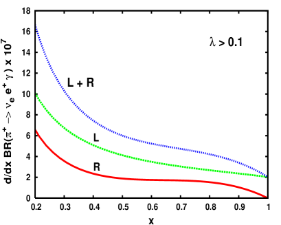
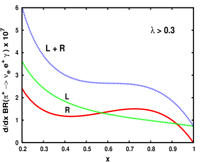
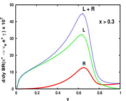
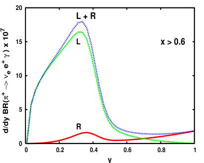
Figure 4: The photon energy spectrum $\frac{\rm dBR_{\gamma}}{\rm dx}$ versus $x$ (top plots) and electron energy spectrum $\frac{\rm dBR_{\gamma}}{\rm dy}$ versus $y$ (bottom plots), for pion decay $\pi^{+}\to\nu_{e}e^{+}\gamma$. The labels $L$ and $R$ attached to the curves indicate pure left-handed and right-handed photon polarizations contributions respectively, while $L+R$ correspond to the sum. Kinematical cuts $\lambda>0.1$ (top-left), $\lambda>0.3$ (top-right) and $x>0.3$ (bottom-left), $x>0.6$ (bottom-right) are applied respectively.

In Fig.4 we show the distributions of BR for pion decay in electron channel. In particular, $d{\rm BR}/dx$ and $d{\rm BR}/dy$ are reported in the “top” and “bottom” plots respectively. In the plots we have integrated the phase space over $\lambda$ and $x$ respectively. Results are obtained by imposing kinematial cuts on $\lambda$ or $x$, as indicated in the plots. Looking at the $d{\rm BR}/dx$ distributions in Fig.4, the general behavior emerging from these results is the following. When cuts on $\lambda$ are relaxed, the left-handed photon polarizations dominate in all range of values of $x>0.2$, corresponding to photon energies $E_{\gamma}>14$ MeV. On the other hand, the contribution of right-handed photons can be increased by imposing larger cuts on $\lambda$, as can be seen by comparing left-top and right-top plots in Fig.4. For example, by requiring that $\lambda>0.3$, right-handed polarizations could dominate in the region of hard photons $0.6<x<0.9$. These results can be explained by using angular momentum conservation. When cuts on $\lambda$ are relaxed, the main contribution to the integral in $d\lambda$ comes from the region of low $\lambda$, where the IB effects dominate with respect to SD terms. Low values of $\lambda$ should correspond to small angles between photons and $e^{+}$, but could also correspond to low positron energies. In the former case, neutrinos are likely to be produced with opposite direction with respect to the photon momentum, in order to compensate for the missing momentum in the pion rest frame. Since neutrinos are always left-handed polarized, photons must be left-handed as well, as required by angular momentum conservation. The spin configuration for this case is shown in Fig.2a. On the other hand, small values of $\lambda$ could also correspond, in the latter case, to the spin configuration shown in Fig.2c, where positron and photon are backward. There, the photon should be mainly emitted from the $\pi^{+}$ line, leaving positron and photon both left-handed polarized. As we will show in section 5, after integrating over $x$ with cuts $x>0.3$, the dominant effect will be given by this last configuration.

On the contrary, when cuts on $\lambda$ are very large, IB effects are reduced and SD terms become sizeable. In this case, the positron is mainly produced right-handed, due to the fact that SD terms are not chiral suppressed, neutrino momentum is favored to be directed forward with respect to the photon one, leading to a right-handed photon as shown in Fig.2b. However, as we can see from the top plots in Fig.4, there is a region of large $x$ where left-handed photon contributions are also sizeable, in particular for $0.9<x<1$. This peculiar behavior in the end point region of photon energy can be explained as follows. When photon energy approaches its maximum, positrons start to be produced almost at rest, if $\lambda$ is small. Then, in order to conserve the total momentum, neutrino should be mainly emitted backward with respect to the photon direction, see Figs.2a and 2c, leading to left-handed photon polarizations as required by angular momentum conservation. However, we should stress that, depending on the cuts on $\lambda$, the right-handed photon polarization could dominate even near the end-point region of photon energy.

In the bottom plots of Fig.4, we report the BRs distributions on positron energy versus $y$, for two representative choices of cuts, namely $x>0.3$ (left-plot) and $x>0.6$ (right-plot). As we can see from these results, the left-handed photon polarizations dominate in the region $y<0.5$, while the gap between left-handed and right-handed contributions increases by using stronger cuts on the photon energies. This behavior can be roughly understood as follows. At fixed positron energy, the larger the photon energy is the more the neutrinos are produced parallel and backward to the photon direction, in order to conserve total momentum. Therefore, as explained above, conservation of angular momentum favors in this case the left-handed photon polarizations. However, at the end point of positron energy, when cuts on $x>0.3$ and $x>0.6$ are imposed, the scenario could be reversed. As a consequence of the strong cuts on $x$, the IB contribution can be made very small, and near the region of $y=y_{max}$, the SD terms should dominate favoring the production of a right-handed positron. Clearly, when photon and positron are both very energetic they tend to be emitted with opposite direction in order to conserve total momentum, approaching, in the case of a right-handed positron, to the spin configuration in Fig.2b. Therefore, due to angular momentum conservation, photons are mainly right-handed in the region $y>0.8$ and $x>0.3$. Here we would like to stress that the relative gap between left- and right-handed contributions of hard photons, near the region $y>0.8$, should be very sensitive to the values of hadronic form factors.

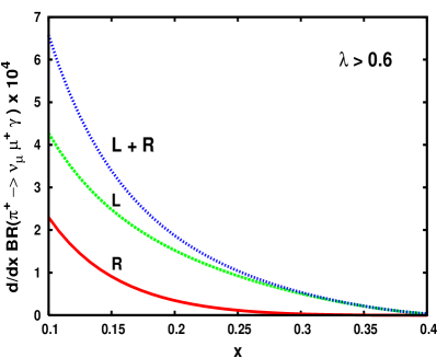
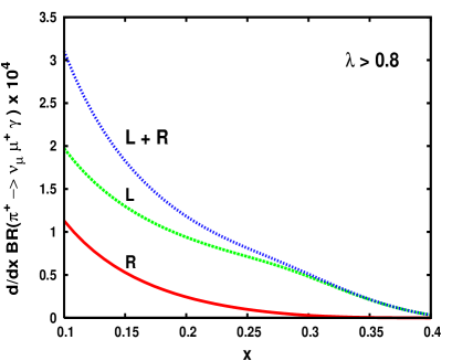
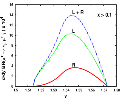
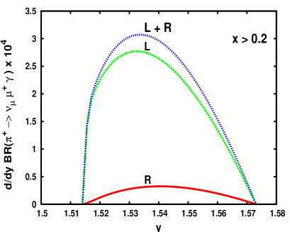
Figure 5: As in Fig. 4, but for pion decay $\pi^{+}\to\nu_{\mu}\mu^{+}\gamma$, and with kinematical cuts $\lambda>0.6$ (top-left), $\lambda>0.8$ (top-right) and $x>0.1$ (bottom-left), $x>0.2$ (bottom-right).

In Fig.5 we show the corresponding results for the pion decay in the muon channel. In this case we can see that the left-handed photon polarizations always dominate over the entire phase space, while right-handed ones are quite suppressed. Notice that, being the muon mass very close to the pion one, the IB contribution is not chiral suppressed as in the electron channel and it is larger than the SD one almost over all the allowed phase space. This implies that $\mu^{+}$ is mainly produced with left-handed polarization. Moreover, due to the fact that here the minimum allowed value of $\lambda$ (for $x>2$) is $\lambda_{\min}\simeq 0.7$, the $\mu^{+}$ and photons are mainly produced at large angles. Then, if left-handed $\mu^{+}$ tends to be produced backward with respect to photon momentum, this last one must be also left-handed in order to conserve total angular momentum, as shown in Fig.2c.

Finally, in Fig.4, we present our results for the $x$- and $y$-distributions of the photon polarization asymmetry, as defined in Eq.(64). In particular, in the top and bottom plots we report the results for the $dA_{\gamma}/dx$ and $dA_{\gamma}/dy$ respectively for several kinematical cuts, while the left and right plots correspond to the electron and muon channel decays respectively. A general property of these results is that the $x$- and $y$-distributions of asymmetry vanish at $x=0$ and $y=1+r_{l}$ respectively. This is a consequence of the fact that when the photon energy is approaching to zero, the polarized photon densities of Dalitz plot tend to the same limit, due to the spin-decoupling property of soft photons, as discussed in section 2. A remarkable aspect of these results is that, in the electron decay channel, the $dA_{\gamma}/dx$ distribution becomes negative for some particular choices of cuts. Analogously, the same effect can be achieved on the $y$-distribution by increasing cuts on the photon energy. On the contrary, in the muon channel, the corresponding asymmetry is always positive, as can be seen in the plots to the right in Fig.6. In conclusion, we would like to emphasize that the position of the zeros of photon polarization asymmetry is particularly sensitive to the effects of the SD terms. This property could suggest a new experimental way for obtaining more precise measurements of form factors.

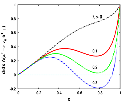
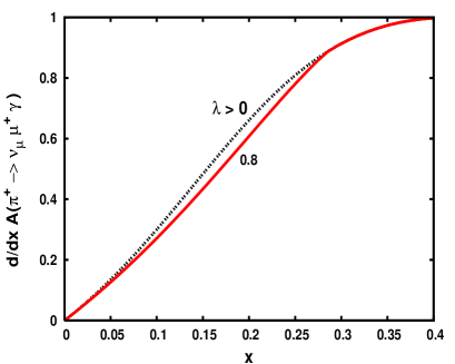
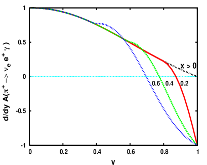
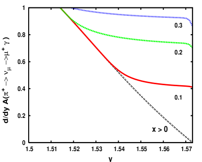
Figure 6: The differential asymmetry $\frac{\rm dA_{\gamma}}{\rm dx}$ versus $x$ (top) and $\frac{\rm dA_{\gamma}}{\rm dy}$ versus $y$ (bottom), with kinematical cuts $\lambda>0,\,0.1,\,0.2,\,0.3$ (top-left), $\lambda>0,\,0.8$ (top-right) and $y>0,\,0.2,\,0.4,\,0.6$ (bottom-left), $y>0,\,0.1,\,0.2,\,0.3$ (bottom-right) respectively.

4.2 Radiative $K^{+}$ decays

In analogy with the radiative pion decays, we analyze here the corresponding ones in the kaon sector, in particular $K^{+}\to e^{+}\nu_{e}\,\gamma$ and $K^{+}\to\mu^{+}\nu_{\mu}\,\gamma$. The expressions of amplitudes in terms of decay constants, masses and form factors remain formally the same as in the pion decay. However, the kaon electromagnetic form factors, as well as the decay constant $f_{K}$, and the ratios $r_{e}$, $r_{\mu}$ between leptons and kaon mass, are quite different from the pion case. As we will see in the following, these differences will sizeably affect the shape of distributions and asymmetries with respect to the corresponding pion decay.

The most recent measurements of $V$ and $A$ form factors have been performed by the E787 collaboration [26] through radiative $K^{+}$ decay $K^{+}\to\mu^{+}\nu_{\mu}\,\gamma$. In particular, the absolute value of $V+A$ has been determined finding $|V+A|=0.165\pm 0.007\pm 0.011$, while a limit on $-0.24<V-A<0.04$ has been set at 90% C.L. These results have been obtained by assuming constant form factors. The $|V+A|$ measurements are consistent with previous results on $K\to e^{+}\nu_{e}\gamma$, but they disagree by almost 2 standard deviations with respect to predictions from leading order in ChPT [12]. We recall here that the evaluation of form factors starts at one loop in ChPT expansion, that is at ${\cal O}(p^{4})$. At this order the chiral prediction, as for the pion case, gives constant form factors. The momentum dependence of the form factors starts then at the next-to-leading order, that is ${\cal O}(p^{6})$, and it is expected to be larger than in pion case, due to sizeable effects of resonances exchange [27]. In particular, by considering only a particular class of diagrams where vector and axial-vector resonances are exchanged, the form factors can be parametrized as

$$V(W^{2})=\frac{V}{1-W^{2}/m_{K^{\star}}^{2}},~{}~{}~{}~{}~{}~{}A(W^{2})=\frac{A}{1-W^{2}/m_{K_{1}}^{2}},~{}~{}~{}~{}~{}~{}$$ (68)

where $W^{2}=m_{K}^{2}(1-x)$, and the masses $m_{K^{\star}}^{2}$ and $m_{K_{1}}^{2}$ correspond to vector and axial-vector resonances. Then, in order to minimize the effects of resonance exchange, large $x$-regions should be considered since $W^{2}\to 0$ when $x\to 1$, while low $x$-regions may be used to explore the $W^{2}$ dependence of $V$ and $A$. The ${\cal O}(p^{6})$ contributions, based on $SU(3)\times SU(3)$ symmetry in ChPT, has been recently calculated in Ref.[28]. Significant deviations of order of 10-20 % have been found on $V$ and $A$ with respect to the leading order calculation. Moreover, while the vectorial form factor is quite sensitive to photon energies, the axial one shows only a modest effect [28].

As for the pion decay, in order to simplify our analysis, we will not take into account the momentum dependence in $V$ and $A$. Then, consistently, we will take the $V,A$ predictions at the leading order in ChPT, re-absorbing the missing NLO contributions in the theoretical uncertainty. In particular, our results are obtained by using the following values [12]

$$V+A=-0.137,~{}~{}~{}~{}~{}~{}~{}~{}~{}V-A=-0.052\,.$$ (69)

In Fig.7 we show the $x-$ (top) and $y-$ (bottom) distributions for the $K^{+}\to e^{+}\nu_{e}\,\gamma$ decay.

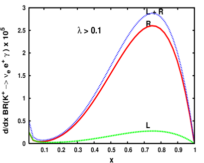
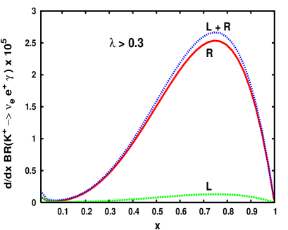
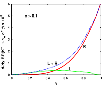
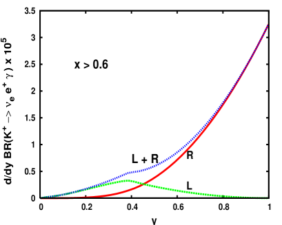
Figure 7: As in Fig. 4, but for kaon decay in $K^{+}\to\nu_{e}e^{+}\gamma$. Curves correspond to kinematical cuts as reported in the figures.

The general trend emerging from these results is that in kaon decay, contrary to the pion case, the right-handed photon production dominates over the lef-handed one, already for moderate cuts $\lambda>0.1$, as can be checked by comparing results between Figs.4 and 7 with the same cuts on $x$ and $\lambda$. This result can be roughly understood as follows. The IB contribution in the radiative $K^{+}$ decay is more “chiral” suppressed with respect to the corresponding $\pi^{+}$ due to the fact that $m_{K}\simeq 4m_{\pi}$. Then, for the same values of $x$ and $\lambda$, the IB effects in pion decay will be larger than in the corresponding kaon one. For instance, while the IB contributions in pion decay are still sizeable after cuts $\lambda>0.1$ and $x>2$ have been imposed, in $K^{+}$ decay these same cuts dramatically reduce the IB effects in favor of SD contributions. As already explained in section 4.1, when the photon is produced from the SD terms it is mainly right-handed polarized. In conclusion, the $d{\rm BR}/dx$ distributions in the top-plots of Fig.7, for $x>0.1$, shows the same behavior of the corresponding one in pion decay in the region $0.6<x<0.9$ and $\lambda>0.3$, where the right-handed photon contributions are enhanced. Moreover, as we can see from the top-plots in Fig.7, these curves have a maximum (for $0.1<x<1$ and $0.1<\lambda<0.3$) around $x\simeq 0.75$. In the bottom-plots of Fig.7 we report the analogous results for the positron energy distributions. As we can see, when the $y>0.5$ and $x>0.1$ cuts are imposed, the right-handed photon gives the dominant effect.

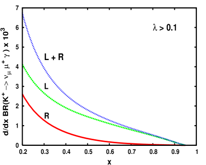
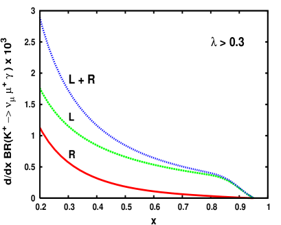
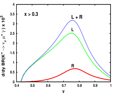
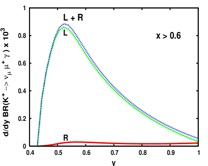
Figure 8: As in Fig. 7, but for kaon decay in $K^{+}\to\nu_{\mu}\mu^{+}\gamma$. Curves correspond to kinematical cuts as indicated in the figures.

In Fig.8 results for BR distributions in $x$ and $y$ are shown for the $K^{+}\to\mu^{+}\nu_{\mu}\gamma$ decay. The hierarchy between L and R curves, and their shapes, are similar to the corresponding ones of $\pi^{+}\to\mu^{+}\nu_{\mu}\gamma$ ( see Fig.7). Notice that the available ranges of $x$ and $y$ are larger for the kaon decay in the muon channel with respect to the corresponding pion decay, due to more available phase space of the former. The same considerations regarding the shapes of $x$- and $y$-distributions of pion decay should hold here as well. As can be seen from these results, also in $K^{+}\to\mu^{+}\nu_{\mu}\gamma$ decay the left-handed photon polarization gives the dominant effect for $x>0.2$ and $\lambda>0.3$ or analogously for $x>0.3$ and $y>0.4$, as shown in the bottom plots for the $y$ distribution. Numerical results for the total contribution L+R, are consistent with the corresponding ones in Ref.[11].

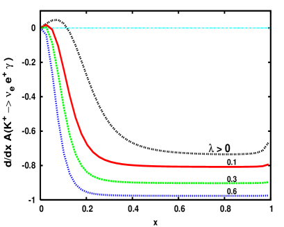
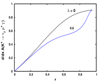
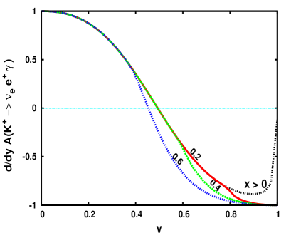
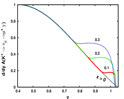
Figure 9: Asymmetries as in Fig. 6, but for kaon decay in $K^{+}\to\nu_{\mu}\mu^{+}\gamma$. Numbers on the curves correspond to kinematical cuts.

In Fig.9 we show our results for the distribution of asymmetries in the kaon decays. As we can see from left-top plots in Fig.9, the $d{\rm A}_{\gamma}/dx$ distribution for $K^{+}\to e^{+}\nu_{e}\gamma$ is always negative in all range $x>0.1$, and tends to a constant value for $x>0.3-0.4$, depending on the applied cuts on $\lambda$. In particular, when $\lambda>0.6$, the $d{\rm A}_{\gamma}/dx$ already approaches its minimum value for $x>0.2$. By relaxing the constraints on $\lambda$, we can see that the $d{\rm A}_{\gamma}/dx$ distribution could have a zero at $x\simeq 0.2$, and analogously $d{\rm A}_{\gamma}/dy$ at $y\simeq 0.5$. On the right-plots we present the corresponding results for the $K^{+}\to\mu^{+}\nu_{\mu}\gamma$ decay, and for some representative choices of cuts. As we can see, the $d{\rm A}_{\gamma}/dx$ is more sensitive to cuts on $\lambda$ than the corresponding one in $\pi^{+}\to\mu^{+}\nu_{\mu}\gamma$. Analogous considerations hold for the $d{\rm A}_{\gamma}/dy$ distribution as well. In conclusion, the photon polarization asymmetry for radiative meson decays in muon channel, is always positive, vanishing only at the end point $x=0$ or analogously $y=1$, due to the spin decoupling property of the soft photon.

4.3 Radiative $\mu^{-}$ decay

In this section we will discuss the numerical results for the radiative muon decay $\mu^{-}\to\nu_{\mu}e^{-}\bar{\nu}_{e}\gamma$. As shown in section 3, this process is described by the leptonic Fermi interaction, where the photon is attached to external legs of muon and electron, see Fig.3. Being a pure leptonic process, its decay rate can be calculated with high accuracy in perturbation theory. In particular, the 1-loop QED corrections have been evaluated in Ref.[15] for the inclusive radiative muon decay, which corresponds to an accuracy of order ${\cal O}(\alpha^{2})$ in the branching ratio. However, studies of polarized radiative muon decays have been recently published [5, 4]. Also 1-loop radiative corrections have been included in the evaluation of the decay rate [4]. However, in these studies only the polarization of fermions has been considered.

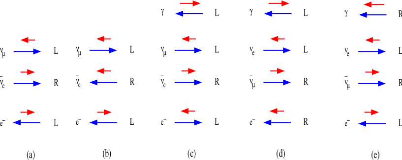
Figure 10: Some helicity (in red) configurations of $\gamma$, $\nu_{\mu}$ $\bar{\nu}_{e}$ and $e^{-}$ for $\mu^{-}\to\nu_{\nu}\bar{\nu}_{e}e^{-}\gamma$ decay in $\mu^{-}$ rest frame, figures (c)-(e), when all momenta (in blue) are aligned on the same axis. Figures (a) and (b) correspond to the non-radiative decay $\mu^{-}\to\nu_{\nu}\bar{\nu}_{e}$. Direction of electron momentum in (a)-(b), as well as photon momentum in (c)-(e) diagrams, is fixed by convention.

Our results for the polarized photon distributions of branching ratios are shown in Fig.11. These results, as well as the corresponding ones in Figs.12 and 15, have been obtained by integrating over the full the phase space and by taking into account the full $r$ dependence.

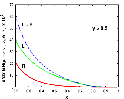
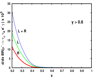
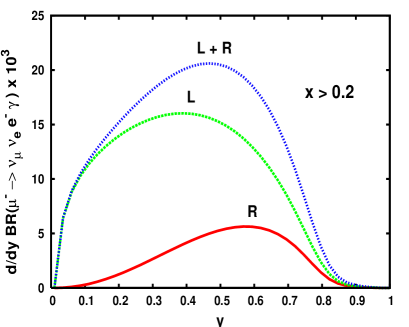
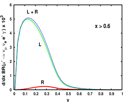
Figure 11: The photon energy ($E_{\gamma}$) spectrum $\frac{\rm dBR_{\gamma}}{\rm dx}$ versus $x=2\,E_{\gamma}/m_{\mu}$ (top) and electron energy ($E_{\gamma}$) spectrum $\frac{\rm dBR_{\gamma}}{\rm dy}$ versus $y=2\,E_{e}/m_{\mu}$ (bottom) for muon decay $\mu^{+}\to\bar{\nu}_{\mu}\nu_{e}e^{+}$ with left-handed (L) and right-handed (R) photon polarizations. and for kinematical cuts $y>0.2$ (top-left), $y>0.6$ (top-right) and $x>0.2$ (bottom-left), $x>0.6$ (bottom-right) respectively.

From Fig.11 we can see that the main contribution to the radiative decay is provided by the left-handed photon polarization, while the right-handed one is quite suppressed and decreases by increasing the photon energy. This behavior, again, can be explained by using angular momentum conservation and parity violation. Notice that, due to the V-A nature of weak interactions, the electron is mainly produced left-handed polarized in the muon decay, and chirality flip effects, needed to produce a right-handed electron, are always sub-leading, being proportional to the electron mass. Moreover, due to the fact that we are integrating over the final phase space of neutrinos, the analysis is strongly simplified. Indeed, after integration, the effect of neutrinos is re-absorbed in the tensor $N^{\alpha\beta}$ appearing in Eqs.(46), (47). Notice that $N^{\alpha\beta}$ is just a projector for the four-momentum $Q^{\alpha}\equiv-(p_{e}+k+p)^{\alpha}$ carried by the neutrinos pair, and it can be seen as the sum over polarization states of a massive particle of spin 1. In other words, regarding the spin content, the neutrinos pair behave as a spin-1 particle of mass $Q^{2}$, having three polarization states. In the case of non-radiative muon decay, the allowed spin configurations in the muon rest frame are shown in Fig.10a,b, where all momenta are aligned on the same axis $X$ and by convention the electron momentum is chosen along the negative direction. As we can see, if the electron is left-handed ($J_{X}=1/2$), the spin projection of neutrino anti-neutrino pair along the direction of their total momentum can be $J_{X}=-1$ or $J_{X}=0$, but not $J_{X}=+1$, being the muon a spin 1/2 particle.

Let us now consider the radiative decay, with photon emission from the electron line. It is known that, when hard photons are emitted parallel and forward to the electron momentum, they can flip the electron helicity, without paying any chiral mass suppression [3, 4, 5, 7, 6, 8]. The helicity-flip mechanism is illustrated below

for incoming left-handed $e_{L}$ (a) and right-handed $e_{R}$ (b) electron by collinear photon bremsstrahlung. All momenta, indicated by blue arrows, are aligned on the same axis. Red arrows stand for the corresponding helicities and an electron mass insertion is understood. We remind here that the chiral suppression of the term $m_{e}^{2}$ appearing in the square modulus of the numerator due to the chirality flip, is compensated by the singular behavior in $\simeq 1/m_{e}^{2}$ appearing in the square modulus of the propagator for collinear photon emission. The corresponding spin configurations in this case are shown in Fig.10d-e for the case of aligned momenta. However, as for the meson case, the contributions coming from the helicity-flip transitions are always smaller with respect to the helicity conserving ones. The largest contributions should come from the photons emitted by the muon line. In this case the neutrinos and electron momenta are favored to be busted backward with respect to the photon momentum, in order to compensate for the missing momentum. The corresponding spin configuration, in the particular limit in which all momenta are aligned on the same axis, is shown in Fig.10c. Since the favored spin of the $\nu+\bar{\nu}$ system is in this case $J_{X}=0$, the photon must be necessarily left-handed polarized. This peculiar configuration should explain why the left-handed photon contribution is always dominant with respect to the right-handed one, leading to an increasing relative gap as the photon energy increases. This seems to be the case since, as the photon energy approaches the soft region $x\to 0$, the gap should decrease due to the spin decoupling property of soft photons. Results concerning the branching ratio distributions for the production of right-handed electron are shown in the next section.

In Fig.12 we show in the right (left) plots the $d{\rm A}_{\gamma}/dy$ ($d{\rm A}_{\gamma}/dx$) distributions asymmetry for the radiative muon decay.

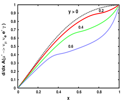
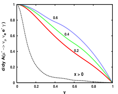
Figure 12: As in Fig.11, but for the asymmetry $\frac{\rm dA_{\gamma}}{\rm dx}$ versus $x$ (left) and $\frac{\rm dA_{\gamma}}{\rm dy}$ versus $y$ (right) and for kinematical cuts $y$ and $x~{}>\{0,\,0.2\,,0.4\,,0.6\}$ for left and right plots respectively.

We present our results for some representative choices of cuts, in particular $y>\{0,~{}0.2,~{}0.4,~{}0.6\}$ and $x>\{0,~{}0.2,~{}0.4,~{}0.6\}$ for the $d{\rm A}_{\gamma}/dx$ and $d{\rm A}_{\gamma}/dy$ respectively. As we can see from these results, the asymmetry in the muon case is always positive, as a consequence of the dominant left-handed photon contribution as discussed above. The shapes of asymmetries are quite similar to the corresponding ones in $\pi^{+}\to\mu^{+}\nu_{\mu}\gamma$ and $K^{+}\to\mu^{+}\nu_{\mu}\gamma$, where the IB effects are larger than the SD terms. In particular, here the $d{\rm A}_{\gamma}/dx$ is monotonically increasing with $x$, while analogously the $d{\rm A}_{\gamma}/dy$ is monotonically decreasing.

5 Energy spectra of the polarized positron/electron

In this section we discuss the results for the distributions of BRs in the positron energy for the decays $\pi^{+}\to e^{+}\nu_{e}\gamma$ and $K^{+}\to e^{+}\nu_{e}\gamma$, and analogously in the electron energy for the radiative muon decay, for both lepton and photons polarizations. As seen before, due to angular momentum conservation, the IB contributions favors a left-handed positron in the soft photon energy region. However, in the case of an hard photon produced collinear with $e^{+}$, the IB favors a right-handed positron. This last effect is due to the helicity-flip mechanism discussed above. However, if one imposes larger cuts on $x$ in order to reduce the IB effect, then the relative contribution of the SD term grows up. In particular, when the positron is totally generated from the SD terms, it is mainly right-handed polarized (see discussions in section 4.1), as can be seen from Eq.(92) in Appendix A, since the photon is emitted from the hadronic vertex. From these results one can easily check that in the region of $y\to 1$, the $LR$ term in Eq.(92) tends to zero and survives only the $RR$ one, corresponding to the production of both positron and photon right-handed polarized, as required by angular momentum conservation. In particular, for a generic meson $M=K,\pi$, we have

$$\lim_{y\to 1}\,\frac{d{\rm BR}^{(R,R)}}{dy}\,\simeq\,{\rm BR}(M^{+}\to l^{+}\nu)\,\frac{\alpha}{2\pi}\frac{(V+A)^{2}}{48\,r_{l}}\frac{m^{2}_{\pi}}{f^{2}_{\pi}}\left(1-4x_{\rm cut}^{3}+3x_{\rm cut}^{4}\right)\,,$$ (70)

where $x_{\rm cut}$ is the cut on $x$, ${\rm BR}(\pi^{+}\to e^{+}\nu)=1.23\times 10^{-4}$ and ${\rm BR}(K^{+}\to e^{+}\nu)=1.55\times 10^{-5}$ [29]. Notice that for a right-handed electron, the contribution from the other polarizations vanishes in the massless lepton limit $r_{l}\to 0$ and for $y\to 1$.

In Fig.13 we show the plots corresponding to the $d{\rm BR}/dy$ of pion decay, where on the left and right plots we report the case of left-handed ($e^{+}_{L}$) and right-handed ($e^{+}_{R}$) positron polarizations respectively.

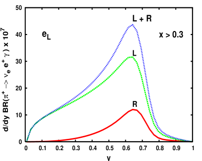
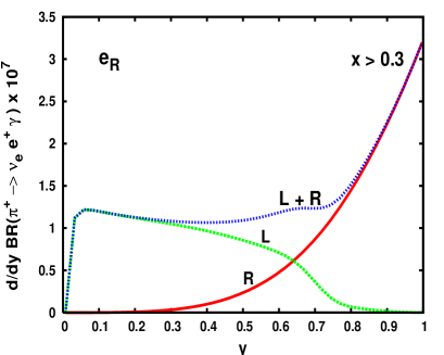
Figure 13: The electron energy spectrum $\frac{\rm dBR}{\rm dy}$ versus $y$ for $\pi^{+}\to\nu_{e}e^{+}\gamma$, for left-handed (left plot) and right-handed electron polarizations (right plot), with photon energy cut $x>0.3$. As in previous figures, the labels $L$ and $R$ labels attached to the curves indicate pure left-handed and right-handed photon polarizations contributions respectively, while $L+R$ correspond to the sum.

These results are obtained for $x>0.3$. As we can see, the contribution of $e^{+}_{L}$ is always dominant with respect to $e^{+}_{R}$ one. This is because the IB effect is still large for $x>0.3$, and so a left-handed positron is favored. Moreover, a peculiar aspect of these results is that for the $e^{+}_{L}$ production, the left-handed photon polarization dominates in all the positron energy range. On the other hand, in $e^{+}_{R}$ distribution, the right-handed photon gives the leading effect for $y>0.7$, being totally induced by the SD terms. The maximum of $d{\rm BR}/dy$ for $e^{+}_{R}$ production, achieved at $y\simeq 1$, can be easily checked by using the approximated expression in Eq.(70).

Analogous results for the kaon decay are shown in Fig.14.

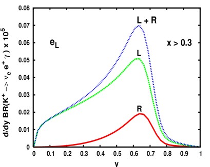
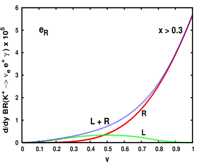
Figure 14: As in Fig.13, but for $K^{+}\to\nu_{e}e^{+}\gamma$.

Here, the situation is reversed with respect to the pion case. The $e^{+}_{R}$ contribution gives the leading effect in the total BR already for $x>0.3$ and the right-handed photon polarization dominates for $y>0.5$. On the other hand, in the $e^{+}_{L}$ distributions (see left plot in Fig.14), the left-handed photon contribution provides the dominant effect. As already mentioned in section 4.2, these differences with pion case are mainly a consequence of the fact that the IB amplitude is more chiral suppressed in $K\to e\nu_{e}\gamma$ than in $\pi\to e\nu_{e}\gamma$.

Finally, in Fig.15 we present the electron energy distributions for the muon case. In this case we imposed a cut $x>0.2$ on the photon energy. We see that in both $e_{R}$ and $e_{L}$ distributions, the left-handed photon contribution always provides the dominant effect, being this configuration favored by angular momentum conservation. Moreover, in the $e_{R}$ case, the right-handed photon contribution is very tiny. As we explained in the previous section, these results are a consequence of the fact that in the radiative muon decay the electron is naturally produced left-handed due to the V-A theory. On the other hand, the contribution of $e_{R}$ is mainly generated from the helicity flip mechanism of hard photons emitted from the electron line and it is a sub-leading effect.

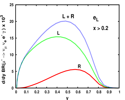
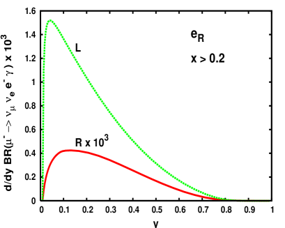
Figure 15: The electron energy spectrum $\frac{\rm dBR}{\rm dy}$ versus $y$ for $\mu^{+}\to\bar{\nu}_{\mu}\nu_{e}e^{+}$, for left-handed (left plot) and right-handed electron polarizations (right plot), with photon energy cut $x>0.2$. The curve in the right plot corresponding to right-handed photon (R), has been multiplied by a rescaling factor of $10^{3}$.

6 Tensorial couplings

Here we analyze the dependence of the photon polarization asymmetry, in the radiative pion and kaon decays, induced by tensorial couplings. The aim of this study is motivated by the recent measurements of the radiative pion decay $\pi^{+}\to\nu_{e}e^{+}\gamma$ [10], where a significant discrepancy in the branching ratio, with respect to the SM predictions [10], has been observed. This anomaly might be interpreted as the effect of a centi-weak tensorial interaction beyond the V-A theory [14].

An analogous discrepancy was noticed long time ago at the ISTRA experiment [22], where radiative pions decays were studied in flight. In that experiment, the $\pi^{+}\to\nu_{e}e^{+}\gamma$ was investigated over a large phase space region, in particular $0.3<x<1$ and $0.2<\lambda<1$. The measured branching ratio $B_{R}^{\rm exp}=(1.6\pm 0.23)\times 10^{-7}$ [22] was found significantly smaller than the expected one $B_{R}^{\rm th}=(2.41\pm 0.07)\times 10^{-7}$, based on the CVC hypothesis and V-A theory of SM. The fact that the measured number of events is less than expected, cannot be explained by a missing unknown background. This result was interpreted [14] as a possible indication of a tensorial quark-lepton interaction with coupling of order $10^{-2}$ in unity of $G_{F}$. In particular, the suggested new contribution to the effective Hamiltonian for $\Delta S=0$ transitions is [14]

$$H_{eff}^{\rm\Delta S=0}=\frac{f_{T}G_{F}}{2\sqrt{2}}\,V_{ud}\left[\bar{u}\sigma_{\mu\nu}(1-\gamma_{5})d\right]\left[\bar{e}\sigma_{\mu\nu}(1-\gamma_{5})\nu_{e}\right]+{\rm h.c.}$$ (71)

where $\sigma_{\mu\nu}=1/2[\gamma_{\mu},\gamma_{\nu}]$ and $f_{T}$ a dimensionless coupling. Notice that tensorial interactions are not subject to the strong constraints coming from the non radiative decay $\pi\to\nu e$ (as, for instance, for the scalar interactions) simply because, the Lorentz covariance forces the hadronic matrix element $\langle 0|\left[\bar{u}\sigma_{\mu\nu}(1-\gamma_{5})d\right]|\pi\rangle$ to vanish. On the other hand, $H_{eff}^{\rm\Delta S=0}$ can contribute to the amplitude ($M_{T}$) of the radiative decay $\pi^{+}\to\nu_{e}e^{+}\gamma$ as

$$M_{T}=i\frac{eG_{F}}{\sqrt{2}}\,V_{ud}\,F_{T}\epsilon^{\mu\star}\,q^{\nu}\left[\bar{e}\sigma_{\mu\nu}(1-\gamma_{5})\nu_{e}\right]\,.$$ (72)

The constant $F_{T}$ can be related to $f_{T}$ in Eq.(71) by using low energy theorems and PCAC hypothesis [14], [30]

$$F_{T}^{0}=\frac{2}{3}\frac{\chi\langle\mu\rangle}{f_{\pi}}\,f_{T}^{0}$$ (73)

where $\langle\mu\rangle=\langle 0|\bar{q}q|0\rangle$ is the vacuum expectation for the quark condensate and $\chi$ is defined by [31]

$$\langle 0|\bar{q}\sigma_{\mu\nu}q|\epsilon(k)\rangle\,=\,e_{q}\chi\,\langle 0|\bar{q}q|0\rangle\,F_{\mu\nu}\,,$$ (74)

with $e_{q}$ the quark $(q)$ electric charge, $F_{\mu\nu}=i(k_{\mu}\epsilon_{\nu}-k_{\nu}\epsilon_{\mu})$, and $\epsilon_{\mu}(k)$ the photon polarization vector of momentum $k$. Then, the destructive interference between the SM and tensorial amplitudes accounts for the correct number of “missing” events observed at ISTRA if $F_{T}=(5.6\pm 1.7)\times 10^{-3}$ [14], corresponding to a tensorial coupling $f_{T}\,\simeq\,(1.4\pm 0.4)\times 10^{-2}$ [30], where $\langle\mu\rangle\,=\,-(0.24\,{\rm GeV})^{3}$ and $\chi\,=\,-(5.7\pm 0.6)\,{\rm GeV}^{-2}$ values have been used [31]. This result is consistent with the limit $f_{T}^{0}<0.095$ (at 68% confidence level) coming from beta decay [14].

Clearly, if confirmed, this effect would be a clear signal of new physics. Indeed, in the SM, the tensorial coupling $f^{SM}_{T}$ is very small, being generated at two-loop level and chiral suppressed. In Ref.[30] the supersymmetric (SUSY) origin of $f_{T}$ has been analyzed. The leading SUSY contribution to $f_{T}$, given by charginos and squarks exchanges in penguin and box diagrams, can be larger than SM one since it is induced at one-loop. However, present bounds on SUSY particle spectra do not allow $f_{T}$ to be larger than $f_{T}\simeq 10^{-4}$, too small for the required value suggested in [14]. Moreover, there have been also criticisms about the consistency of such large tensorial couplings. In Ref.[32] it was pointed out that, due to QED corrections, an $f_{T}$ of order of ${\cal O}(10^{-2})$ might run in troubles. Indeed, the operator in Eq.(71) can mix under QED radiative corrections with a scalar operator, whose contribution is strongly constrained by $\pi^{+}\to e^{+}\nu_{e}$ [32]. In particular, an upper bound on $f_{T}<10^{-4}$ can be set by imposing the strong constraints on scalar interactions coming from $\pi^{+}\to e^{+}\nu_{e}$, which is two order of magnitude smaller than the required one [14]. However, more accurate analyses showed that it is possible to relax or even avoid the upper bound claimed in [32]. For instance, the simultaneous (fine-tuned) contributions of both tensorial and scalar interactions, as suggested by lepto-quark models [33], might relax the upper bound in [32] and thus the interpretation given in [14] cannot be regarded yet as ruled out. There is also an alternative solution, proposed in Ref.[34], where a modified tensorial interaction can formally avoid the mixing with scalar operator, while solving the ISTRA discrepancy.

In Ref.[11], it was pointed out that an analogous effect might show up in the kaon sector. In particular, if the origin of $f_{T}$ is flavour independent, then a tensorial interaction of the same order is also expected in the $\Delta S=1$ transitions, leaving to a large anomaly in radiative kaon decays, easily detected at present and future kaon factories [11].

Recently, the PIBETA collaboration at Paul Scherrer Institute facility, has performed an accurate analysis of the $\pi^{+}\to\nu_{e}e^{+}\gamma$ decay [10] using a stopped pion beam. More than 40,000 $\pi^{+}\to\nu_{e}e^{+}\gamma$ events have been collected, allowing for a very precise measurement of the branching ratio. In this experiment, a more significant discrepancy (about $8\sigma$ [35]) between data and SM predictions has been reported in the kinematical region of high-energy photon/low-energy positron. A significant number of expected events are missing. As for the ISTRA anomaly, agreement with data can be improved by adding a negative tensor term $F_{T}\simeq-0.002$, a bit smaller (in magnitude) than the corresponding one in [14]. More detailed analysis about the PIBETA experiment can be found in [36] and references therein.

Now we analyze the impact of a tensorial coupling on the photon polarization asymmetry $d{\rm A}_{\gamma}/dx$ in radiative pion and kaon decays. In order to simplify the analysis, we will assume an universal tensorial interaction in both $\Delta S=0,1$ processes, parametrizing all the effects in a phenomenological coupling $F_{T}$ as follows

$$M_{T}=i\frac{eG_{F}}{\sqrt{2}}F_{T}\,V_{uq}\epsilon^{\mu\star}_{L}\,q^{\nu}\left[\bar{e}\sigma_{\mu\nu}(1-\gamma_{5})\nu_{e}\right]\,,$$ (75)

where $q=d$ and $q=s$ for pion and kaon decays respectively. As discussed in section 1, the photon emitted by the tensorial amplitude $M_{T}$ in Eq.(75) is purely left-handed. This property can also be checked by noticing that the interference between $M_{T}$ and $M_{\scriptscriptstyle SD}$ terms is proportional to the $V-A$ combination [14]. Below we provide the additional tensorial contributions to the (photon) polarized Dalitz plot density. In particular, the following term $\rho^{(-1)}_{T}(x,\lambda)$ should be added to $\rho^{(-1)}(x,\lambda)$ in Eq.(17)

$$\rho^{(-1)}_{T}(x,\lambda)=2\,A_{\scriptscriptstyle SD}F_{T}\left(F_{T}f_{\scriptscriptstyle TT}(x,\lambda)+2\sqrt{r_{l}}\frac{f_{M}}{m_{M}}\,f_{\scriptscriptstyle IBT}(x,\lambda)+\sqrt{r_{l}}\,(V-A)f_{\scriptscriptstyle SDT}(x,\lambda)\right)$$ (76)

where [11]

$$f_{\scriptscriptstyle TT}(x,\lambda) = \lambda\,x^{3}(1-\lambda),~{}~{}~{}f_{\scriptscriptstyle IBT}(x,\lambda)=x\left(1+r_{l}-\lambda-\frac{r_{l}}{\lambda}\right),~{}~{}~{}$$

$$f_{\scriptscriptstyle SDT}(x,\lambda) = x^{3}\left(1-\lambda\right)\,.$$ (77)

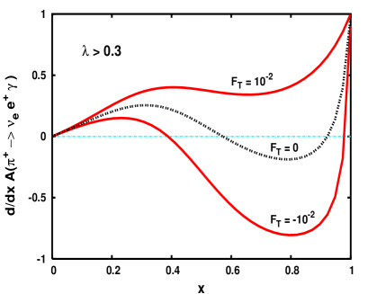
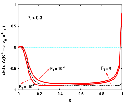
Figure 16: Photon polarization asymmetry $d{\rm A}_{\gamma}/dx$ versus $x$ and with $\lambda>0.3$, for two values of tensorial coupling $F_{T}=\pm 10^{-2}$. Left and right plots correspond to $\pi^{+}\to\nu_{e}e^{+}\gamma$ and $K^{+}\to\nu_{e}e^{+}\gamma$ decays respectively. The dark dashed curves stand for the standard model case ($F_{T}=0$).

In Fig.16 we show the $d{\rm A}_{\gamma}/dx$ asymmetry versus $x$, for two representative values of $F_{T}=\pm 10^{-2}$ and cut $\lambda>0.3$, for the $\pi^{+}\to\nu_{e}e^{+}\gamma$ (left plot) and $K^{+}\to\nu_{e}e^{+}\gamma$ (right plot). As we can seen from these results the shape of photon asymmetry is quite sensitive to a tensorial coupling in the range of $|F_{T}|\simeq 10^{-2}$. In particular, in the pion case, this sensitivity is more pronounced, and the position of zeros of the asymmetry strongly depend on $F_{T}$. On the other hand, in the kaon decay, large deviations should appear only in the region of large $x$, where the tensorial effect is enhanced. This difference in the two decays can be explained due to the fact that the tensorial interference, which is the dominant effect when $F_{T}<10^{-2}$, is always chiral suppressed, being proportional to $m_{e}/m_{M}$. Thus, in the radiative kaon decay, this effect is more suppressed than in the pion case, due to the larger meson mass. We have explicitly checked that, in the corresponding pion and kaon decays in muon channel, the sensitivity of the asymmetry to $F_{T}$ is very modest and we do not show the corresponding results. In conclusion, we suggest that the possibility to measure the photon polarization in pion, or even in kaon decays, could be very useful to clarify the controversial question of tensorial

7 Cancellation of mass singularities

In this section we discuss the mechanism of mass singularities cancellation and the way it takes place in meson and muon polarized radiative decays. As will be seen a new peculiar cancellation pattern shows up in the particular case of the polarized amplitudes differently from the well known cancellation taking place in the inclusive unpolarized amplitudes.

In a theory with massless particles a crucial test of the consistency of the computation is represented by the absence of mass singularities in any obtained physical quantity. Mass singularities are of two types: infrared and collinear. Infrared divergences originate from massless particles with a vanishing momentum in the small energy soft limit. Physical states as, for example, a single charged particle, are degenerate with states made by the same particle accompanied by soft photons. This corresponds to the impossibility of distinguishing a charged particle from the one accompanied by given number of soft photons due to the finite resolution of any experimental apparatus. An infrared divergence appears in QED when the energy $E_{\gamma}$ of the photon goes to zero as a factor of the form:

$$I=\int_{0}^{1}\frac{d\epsilon}{\epsilon}$$ (78)

where $\epsilon=\frac{E_{\gamma}}{E}$ is the fraction of the energy of the photon with respect to the total available energy ${E}$ for the process. The Bloch Nordsiek theorem [37] assures the cancellation of infrared divergences in any inclusive cross section. Collinear divergences, instead, come from massless particles having a vanishing value of the relative emission angle. In QED, specifically, when one or more photons, in the limit of zero fermion mass, are in a collinear configuration i.e. with emission angle $\theta\simeq 0$. Physical states containing a massless charged particle are degenerate with states containing the same particle and a number of collinear photons. Any experimental apparatus, having a finite angular resolution, cannot distinguish between them. The angular separation of two massless particles with momenta $p$ and $k$ is such that they move parallel to each other with a combined invariant mass for $\theta\rightarrow 0$:

$$q^{2}=(p+k)^{2}=2\,{p_{0}}\,{E_{\gamma}}(1-\cos\theta)\rightarrow\;0$$ (79)

even though neither $p$ nor $E_{\gamma}$ are soft. Here $\theta$ is the emission angle of a photon with respect to the fermion. The inclusive procedure of integrating over the photon emission angles by keeping the fermion mass finite does not give rise to any collinear singularity. The divergence appears in the limit $\theta\rightarrow 0$ as the presence of a logarithm of the form $\log(\frac{E}{m})\simeq\log(\theta)$.

For collinear singularities, as well as for infrared ones, the case for inclusive unpolarized processes is well known and it is governed by the Kinoshita-Lee-Nauenberg (KLN) theorem [38]. For the collinear singularities the KLN theorem guarantees that collinear divergences cancel out if one performs a sum of the amplitude over all the sets of degenerate states order by order in the perturbative expansion. For the amplitude of a single photon emission a combination of collinear and infrared singularities gives, for instance, contributions of the type:

$$R=\frac{\alpha}{\pi}\;\int_{0}^{1}\;\frac{d\epsilon}{\epsilon}\;\int_{0}^{1}\;\frac{d\theta}{1-\cos\theta}\,.$$ (80)

In order to discuss the above aspects on the cancellation of lepton mass singularity in the polarized pion decay, we first recall the mechanism taking place in the unpolarized case [39, 40]. In general, the decay rate is made free from mass singularities in the ordinary way: the cancellation of divergences occurs in the total inclusive decay rate at order ${\cal O}(\alpha)$, namely in the pion case

$$\Gamma^{\rm(incl)}=\Gamma(\pi\to\nu e)+\Gamma(\pi\to\nu e\gamma)\,,$$ (81)

when the full ${\cal O}(\alpha)$ order contributions are included, i.e. those relative to real and virtual photon emission [39, 40]. However, for a pointlike (structureless) pion, due to the chirality flip of final charged lepton, the pion decay amplitude is always proportional to $m_{l}$ and vanishes in the $m_{l}\to 0$ limit. In other words, in the limit $m_{l}\to 0$ the decay rate is made finite from mass singularities in a trivial way. For example, as we will see later on, a term proportional to ${\rm Log}(m_{l})$ will remain in the inclusive width due to the mass renormalization of the charged lepton in the virtual contributions to $\Gamma(\pi\to\nu e)$. However, since it will be multiplied by $m_{l}^{2}$, it will give no troubles since $\Gamma_{0}\to 0$ tends to zero at the same time. However, as pointed out by Kinoshita in [39], the leading ${\log}(m_{l})$ terms in the IB contribution to $\Gamma(\pi\to\nu e\gamma)$ cancel out exactly when one adds the virtual contributions. In other words, the mass singularities in the ${\log}(m_{l})$ terms should cancel independently from the fact that the effective coupling in the pion decay is proportional to the charged lepton mass or not. The cancellation mechanism of these Log terms shows a non trivial aspect of the KLN theorem in the pion decay. For this reason, in the following discussion we will consider the following ratios $\Gamma(\pi\to\nu e\gamma)/\Gamma_{0}$ and $\Gamma(\pi\to\nu e)/\Gamma_{0}$ which survives the limit $m_{l}\to 0$.

Let us now consider the case of radiative polarized decays within the soft and collinear region for the radiated photon. We will investigate in this section the mechanism which will assure the finiteness of the lepton distribution against the appearance of infrared and collinear singularities on the above ratios of widths. Let us start by the inclusive distributions in terms of the final lepton energy $y$ as listed in Eq.(88). The Inner Bremsstrahlung contribution contained in Eq.(91) in the $r_{l}\rightarrow 0$ limit is composed by the four expressions corresponding to the various polarization states of the final photon and lepton respectively. The last, $RR$ polarized term is identically zero. The remaining three are related to the left-handed ( first and third ) and right-handed ( second ) lepton respectively.

The logarithms $L_{1},L_{2}$ do correspond to collinear contributions. By integrating the double-inclusive distribution of Eq.(85) one gets in the expression of Eq.(89) for the $IB$ case that the expressions for $F^{(\lambda_{\gamma},\lambda_{l})}_{i}(y)$ depend on the logarithms $L_{1}$ and $L_{2}$ respectively

$$L_{1}=\log{\left(\frac{y+{\rm A}_{l}-2\,r_{l}}{y-{\rm A}_{l}-2\,r_{l}}\right)},~{}~{}~{}~{}~{}~{}~{}~{}L_{2}=\log{\left(\frac{y+{\rm A}_{l}-2}{y-{\rm A}_{l}-2}\right)}$$

These terms do give rise to two kinds of “collinear” logarithms:

$$L_{1} = \log\frac{E_{l}}{m_{l}},~{}~{}~{}~{}~{}~{}~{}~{}L_{2}=\log\frac{E_{l}+\sqrt{E_{l}^{2}+m_{l}^{2}}-m_{M}}{E-\sqrt{E_{l}^{2}+m_{l}^{2}}-m_{M}}\,.$$

The first logarithm represents the case of the photon being parallel to the lepton, the second collinear logarithm for $m_{l}\rightarrow 0$ and $m_{M}\rightarrow 0$ corresponds to the case where the photon is parallel to the decaying meson [3]. Clearly, it is only $L_{1}$ which is affected by the true collinear divergence in the limit $m_{l}\to 0$.

With respect to the unpolarized inclusive case some differences are worth to be noticed here:

• Different polarization amplitudes do represent independent observables in the decay. Therefore if we consider the two cases of a right-handed and left-handed lepton they have to be also separately finite.

• At zero order in the pion decay the angular momentum conservation imposes to the lepton to be left-handed. By radiating a photon a total zero angular momentum is assigned to the final state even if a right-handed lepton emits a left-handed polarized photon. This contribution is represented by the second term in Eq.(91).

• For $y\rightarrow 1$ only the second term in Eq.(91), corresponding to the $LR$ polarization, contribution is finite, i.e. it is zero:

  $$\lim_{{r_{l}\to 0}\;\;{y\to 1}}\frac{1}{\Gamma_{0}}\frac{d\Gamma_{\scriptscriptstyle IB}^{(\rm L,R)}}{dy}=\frac{\alpha}{2\pi}\Big{(}1-y\Big{)}=0\,.$$

This fact shows that the $LR$ term, corresponding to the anomalous term [41], it is finite by itself without the need of any cancellation mechanism in the infrared $y\rightarrow 1$ and collinear limit $r_{l}\rightarrow 0$. A detailed discussion of the undergoing dynamics can be found in Ref.[3]

Analogous conclusions, regarding the finiteness of the right-handed lepton contribution in the $r_{l}\rightarrow 0\,,y\rightarrow 1$ limits to the structure dependent terms $|SD|^{2}$ and the $IB\times SD$, see Eqs.(92) and (93) respectively, hold there as well.

Let us now consider the contributions of the type $LL$ and $RL$ giving rise to a left handed lepton. Manifestly the first and third term of Eq.(91) are divergent in the $r_{l}\rightarrow 0\;,~{}y\rightarrow 1$ limits. The expression obtained by adding first and third contributions in Eq.(91) is:

$$\frac{1}{\Gamma_{0}}\Big{[}\frac{d\Gamma_{\scriptscriptstyle IB}^{(\rm L,L)}}{dy}+\frac{d\Gamma_{\scriptscriptstyle IB}^{(\rm R,L)}}{dy}\Big{]}=\frac{\alpha}{2\pi}\,\frac{1}{y-1}\Big{[}\Big{(}1+y-{\hat{L}}_{1}-{\hat{L}}_{2}\Big{)}+\Big{(}y\left(y+1\right)-{\hat{L}}_{1}\,y^{2}+{\hat{L}}_{2}\left(1-2\,y\right)\Big{)}\Big{]}$$

which is divergent both in the collinear and in the infrared limit. The coefficients of the collinear logarithms remain different from zero as $r_{l}\rightarrow 0$ and $y\rightarrow 1$, leaving to a divergent expression. As for the unpolarized case for the left-handed lepton contributions one needs to consider the additional virtual contributions in order to cancel infrared singularities [39].

The case of the left-handed lepton includes also the diagram of the virtual photon i.e. the one with a photon line connecting meson and charged lepton. This diagram does not add any angular momentum to the zeroth order term since a virtual particle does not add angular momentum to the final state. The amplitude containing the virtual photon gives rise, therefore, to a lepton neutrino final state having the same helicities as the ones of the tree level amplitude. The combination of real and virtual contributions should, in the left-handed lepton channel, add among each other to give a finite result. This mechanism is the same taking place for the cancellation of singularities for the inclusive, unpolarized amplitudes as we will discuss in more details below.

According to [39] the total width for the unpolarized IB contribution to $\Gamma(\pi\to\nu e\gamma)$ is given by

$$\frac{\Gamma_{IB}(x_{0})}{\Gamma_{0}} = \frac{\alpha}{\pi}\Big{\{}b(r_{l})\left(\log{\frac{x_{0}}{2}}-\log(1-r_{l})-\frac{1}{4}\log(r_{l})+\frac{3}{4}\right)$$ (82)

$$- \frac{r_{l}\left(10-7r_{l}\right)}{4\left(1-r_{l}\right)^{2}}\log(r_{l})+\frac{2\left(1+r_{l}\right)}{1-r_{l}}L(1-r_{l})+\frac{15-21r_{l}}{7(1-r_{l})}\Big{\}}\,,$$

where $x_{0}$ is the minimum photon energy which regularizes the infrared divergence in the photon mass, the function $b(x)=\frac{1+x}{(1-x)}\log(x)+2$, and $L(x)=\int_{0}^{x}\log(1-t)dt/t$. For a generalization of the result in Eq.(82) to the inclusion of the leading logarithmic terms to all orders in perturbation theory see Ref.[42, 43, 44].

For the virtual 1-loop contribution one has to consider the radiative corrections to the operator $gm_{l}^{0}Q$, where $Q=\bar{\psi}_{l}(1-\gamma_{5})\psi_{\nu}\varphi_{\pi}$, with $\varphi_{\pi}$ is the pion field and $m_{l}^{0}$ is the ‘bare’ mass of the charged lepton. These corrections split in two separate contributions: $\Gamma^{(1)}$ given by the correction to the operator $Q$ and $\Gamma^{(2)}$ arising when one try to express the bare mass $m_{l}^{0}$ in terms of the renormalized lepton mass $m_{l}$, namely $m_{l}^{0}=m_{l}-\delta m_{l}$ with $\delta m_{l}=\frac{3\alpha}{2\pi}m_{l}\left(\log(\Lambda/m_{l})+\frac{1}{4}\right)$ [40]. For $\Gamma^{(1)}$, one has [39]

$$\frac{\Gamma^{(1)}}{\Gamma_{0}}=\frac{\alpha}{\pi}\,\left\{-b(r_{l})\left(\log(\frac{x_{0}}{2})-\frac{1}{4}\log(r_{l})+\frac{3}{4}\right)+\frac{r_{l}}{2(1-r_{l})}\log(r)+\frac{1}{2}\right\}+\frac{3\alpha}{2\pi}\log(\frac{\Lambda}{m_{\pi}})$$ (83)

Notice that the last term, containing the ultraviolet cut-off $\Lambda$ needed to regularize the UV divergency, can in principle be absorbed in a re-definition of $f_{\pi}$ at order $\alpha$, see Ref.[40] for more details.

As can be seen by comparing the results in Eqs.(82) and (83), the $\log{r_{l}}$ terms surviving the limit $r_{l}\to 0$ cancel out in the sum of virtual and real emission contributions as a consequence of the KNL theorem. Finally, for the total contribution to the unpolarized inclusive decay rate at order $\alpha$, including the contribution of $\Gamma^{(2)}$, one gets [39, 40]:

$$\frac{\Gamma^{(\rm incl)}}{\Gamma_{0}}=1+\frac{\alpha}{\pi}\,\Big{\{}\frac{3}{2}\log(r_{l})+\frac{13}{8}-\frac{\pi^{2}}{3}\,\Big{\}}\,,$$ (84)

where we retained only the leading terms in $m_{e}\to 0$ limit. As previously mentioned, the appearance of the $\log{r_{l}}$ term in (84) is due to the renormalization of the charged lepton mass which does not follow the same pattern of collinear mass singularities discussed above [39]. For simplicity, we omitted in (84) the term containing a $\log(\Lambda/m_{\pi})$, since it can be absorbed into a re-definition of $f_{\pi}$ at order $\alpha$ inside $\Gamma_{0}$.

As stated above, in the right-handed case, on the contrary, the mass singularities cancellation occurs with a different mechanism. Infrared and collinear limits in the ratio $\Gamma_{IB}^{(LR)}/\Gamma_{0}$ give separately a finite result. In particular, the coefficient of the collinear logarithms for the right handed lepton case is the lepton mass, instead of the usual correction factor coming from the soft and the virtual photon contributions.

The particular cancellation mechanism occurring in the right-handed radiative decay is originated by the combined constraints of the angular momentum conservation in the pion vertex and the one of the helicity flip in the photon-lepton vertex [3].

Let us now consider the case of the muon decay. As shown in Eq.(57) as for the meson case also in the muon decay lepton distribution we see that the $LR$-photon-lepton polarized distribution is free from collinear and infrared singularities and goes to zero in the infrared limit $y\rightarrow 1$. The remaining $RL$ and $LL$ distributions, apart from the identically zero $RR$ term, do give a finite contributions in the $y\rightarrow 1$ limit, provided that the same $x_{0}$ cut-off is also set free to go to the soft kinematical limit i.e. $x_{0}\rightarrow 0$. In the muon case the pattern of singularities cancellation repeats itself as for the meson case.

8 Conclusions

We have computed polarized distributions in radiative meson and muon decays, by taking into account final lepton and photon helicity degrees of freedom. The definition of photon polarization asymmetry has been introduced, allowing a new approach to investigate interaction dynamics via a finite and universal quantity directly associated to parity violation. Analytical and numerical results for the polarized distributions and branching ratios, as well as for the photon polarization asymmetry, have been explicitly derived.

The main results of the photon polarization analysis in meson decays, inclusive in the spin degrees of freedom of the final lepton, can be summarized as follows. In the pion case, the production of hard photons in association with soft positrons, are mainly favored to be left-handed polarized. However, when the positron energy increases, the relative gap between left-and right-handed photons decreases, due to the increasing contributions of hadronic structure dependent terms. Remarkably, in the kaon decay, when energy cuts $E_{\gamma}\raise 1.29167pt\hbox{$\;>$\kern-7.5pt\raise-4.73611pt\hbox{$\sim\;$}}25$ MeV and $E_{e^{+}}\raise 1.29167pt\hbox{$\;>$\kern-7.5pt\raise-4.73611pt\hbox{$\sim\;$}}120$ MeV are imposed, both photon and positron are mainly right-handed polarized and a large and negative photon polarization asymmetry is expected. Regarding the corresponding meson decays in muon channel, the left-handed photon production always gives the leading effect. The same behavior is observed in the radiative muon decay $\mu^{-}\to\nu_{\mu}e^{-}\bar{\nu}_{e}\,\gamma$. All these results can be easily explained in terms of angular momentum conservation and parity violation.

We have also systematically analyzed the mechanisms of cancellation of infrared and collinear divergences in polarized meson and muon decays. It has been shown that the finiteness of the polarized amplitudes takes place in a different way for left- with respect to right-handed final leptons when inclusive results in the photon polarization degrees of freedom are taken into account.

Finally, we propose a possible test using photon polarization in order to solve the controversial issue of large tensorial couplings in lepton-quark interactions, as suggested by the recent observed anomaly at the PIBETA experiment. In particular, it is argued that the measurement of the photon polarization asymmetry may constitute a sensible test to resolve such controversial issue in radiative pion decay, providing a sensitive probe to hadronic form factors as well as to new physics effects in meson radiative decays.

We believe that all these new results could open a more extended perspective into the physics of the semileptonic weak decays. In particular, the less inclusive approach to the polarized processes, by explicitly taking into account lepton and photon polarization degrees of freedom, could allow, when the experimental conditions make it compatible, a new quantitative approach and a more detailed inspection of meson and muon decays. Moreover, we are confident that Standard Model physics as well as signals of physics beyond the Standard Model could be put under scrutiny and more closely investigated by using tests involving polarized quantities.

Appendix A

Here we provide the most general results for the polarized meson radiative decay in the meson rest frame, as a function of $x,y$ variables defined in Eq.(19), and for both charged lepton $l=e,\mu$ and photon helicities $\lambda_{l}$ and $\lambda_{\gamma}$ respectively. For later convenience, we will use the same notation adopted in section 2, where the symbols $L$ and $R$ are associated to particle helicities $\lambda=-1$ and $\lambda=1$ respectively. In particular, for the differential radiative decay rate normalized to its non radiative one, we obtain

$$\frac{1}{\Gamma_{0}}\frac{d^{2}\Gamma^{(\lambda_{\gamma},\lambda_{l})}}{dx\,dy}=\frac{\alpha}{2\pi}\frac{1}{(1-r_{l})^{2}}\,\rho^{(\lambda_{\gamma},\lambda_{l})}(x,y)$$ (85)

where

$$\rho^{(\rm L,\lambda_{l})}(x,y) = f_{\scriptscriptstyle IB}^{(\rm L,\lambda_{l})}(x,y)+\frac{m_{M}^{2}}{f_{M}^{2}}\frac{(V-A)^{2}}{4\,r_{l}}f_{\scriptscriptstyle SD}^{(\rm L,\lambda_{l})}(x,y)+\frac{m_{M}}{f_{M}}(V-A)\,f_{\scriptscriptstyle INT}^{(\rm L,\lambda_{l})}(x,y)~{}~{}~{}$$

$$\rho^{(\rm R,\lambda_{l})}(x,y) = f_{\scriptscriptstyle IB}^{(\rm R,\lambda_{l})}(x,y)+\frac{m_{M}^{2}}{f_{M}^{2}}\frac{(V+A)^{2}}{4\,r_{l}}f_{\scriptscriptstyle SD}^{(\rm R,\lambda_{l})}(x,y)+\frac{m_{M}}{f_{M}}(V+A)\,f_{\scriptscriptstyle INT}^{(\rm R,\lambda_{l})}(x,y)~{}~{}~{}$$

where the functions $f_{IB}^{(\lambda_{\gamma},\lambda_{l})}(x,y)$, $f_{SD}^{(\lambda_{\gamma},\lambda_{l})}(x,y)$, and $f_{INT}^{(\lambda_{\gamma},\lambda_{l})}(x,y)$ are given by

$$f_{\scriptscriptstyle IB}^{(L,\lambda_{l})}(x,y) = \frac{1-y+r_{l}}{2\,{\rm A}_{l}\,{x^{2}}\,{z^{2}}}\,\Big{\{}{\rm A}_{l}\,\left(\,x+y-1+r_{l}\,\left(\,-3x-y+x\,y\right)+{r_{l}^{2}}\right)$$

$$- \lambda_{l}\left[y\,\left(x+y-1\right)+r_{l}\,\left(4-6\,x-6\,y+3\,x\,y+{y^{2}}-x\,{y^{2}}\right)\right.$$

$$+ \left.{r_{l}^{2}}\,\left(4+2\,x-y\right)\right]\Big{\}}$$

$$f_{\scriptscriptstyle IB}^{(R,\lambda_{l})}(x,y) = \frac{1-y+r_{l}}{{2\,{\rm A}_{l}\,{x^{2}}\,z^{2}}}\,\Big{\{}{\rm A}_{l}\,\left(x-1+r_{l}\right)-\lambda_{l}\Big{[}\left(x-1\right)\,y-r_{l}\,\left(2\,x+y-4\right)\Big{]}\Big{\}}$$

$$\times \Big{\{}\left(x-1\right)\,\left(x+y-1\right)+r_{l}\Big{\}}$$

$$f_{\scriptscriptstyle SD}^{(L,\lambda_{l})}(x,y) = \frac{1-y+r_{l}}{2{\rm A}_{l}}\,\Big{\{}{\rm A}_{l}\,\left(\left(x-1\right)\,\left(y-1\right)+r_{l}\right)$$

$$- \lambda_{l}\Big{[}y\,\left(x+y-1-x\,y\right)+r_{l}\,\left(2\,x-y\right)\Big{]}\Big{\}}$$

$$f_{\scriptscriptstyle SD}^{(R,\lambda_{l})}(x,y) = \frac{(x-1)(x+y-1)+r_{l}}{2{\rm A}_{l}}\,\Big{\{}{\rm A}_{l}\left(1-x-y+r_{l}\right)$$

$$- \lambda_{l}\Big{[}y\left(x+y-1\right)-r_{l}\left(2x+y\right)\Big{]}\Big{\}}$$

$$f_{\scriptscriptstyle INT}^{(L,\lambda_{l})}(x,y) = \frac{1-y+r_{l}}{2\,{\rm A}_{l}\,xz}\,\Big{\{}{\rm A}_{l}\,\left(1-2\,x-y+x\,y+r_{l}\right)$$

$$- \lambda_{l}\Big{[}2-2\,x-3\,y+2\,x\,y+{y^{2}}-x\,{y^{2}}+r_{l}\,\left(2+2\,x-y\right)\Big{]}\Big{\}}$$

$$f_{\scriptscriptstyle INT}^{(R,\lambda_{l})}(x,y) = \frac{1-y+r_{l}}{2\,{\rm A}_{l}\,xz}\,\Big{\{}{\rm A}_{l}+\lambda_{l}\Big{[}2\,x+y-2\Big{]}\Big{\}}\,\Big{\{}\left(1-x\right)\,\left(x+y-1\right)-r_{l}\Big{\}}$$ (86)

where $\lambda_{l}=1$ and $\lambda_{l}=-1$ correspond to right- (R) and left-handed (L) fermion polarization respectively, and symbols $\Gamma_{0}=\Gamma(M^{+}\to\nu_{l}l^{+})$, $z=x+y-1-r_{l}$, and ${\rm A}_{l}=\sqrt{y^{2}-4r_{l}}$.

By integrating equations above in the photon energy $x$ range

$$1-\frac{1}{2}\left(y+{\rm A}_{l}\right)\,\leq\, x \,\leq\,1-\frac{1}{2}\left(y-{\rm A}_{l}\right)$$

$$2\sqrt{r_{l}}\,\leq y \,\leq\,1+r_{l}\,,$$ (87)

we obtain

$$\frac{1}{\Gamma_{0}}\frac{{d\Gamma}^{(\lambda_{\gamma},\lambda_{l})}}{dy} = \frac{\alpha}{2\pi}\frac{1}{(1-r_{l})^{2}}F^{(\lambda_{\gamma},\lambda_{l})}(y)$$ (88)

where

$$F^{(L,\lambda_{l})}(y) = \frac{F^{(L,\lambda_{l})}_{\scriptscriptstyle IB}(y)}{2{\rm A}_{l}\left(1-y+r_{l}\right)}+\frac{m_{M}^{2}}{f_{M}^{2}}\frac{(V-A)^{2}}{4\,r_{l}}\,F^{(L,\lambda_{l})}_{\scriptscriptstyle SD}(y)+\frac{m_{M}}{f_{M}}\,(V-A)\,\frac{F^{(L,\lambda_{l})}_{\scriptscriptstyle INT}(y)}{2\,{\rm A}_{l}}$$

$$F^{(R,\lambda_{l})}(y) = \frac{F^{(R,\lambda_{l})}_{\scriptscriptstyle IB}(y)}{2{\rm A}_{l}\left(1-y+r_{l}\right)}+\frac{m_{M}^{2}}{f_{M}^{2}}\frac{(V+A)^{2}}{4\,r_{l}}\,F^{(R,\lambda_{l})}_{\scriptscriptstyle SD}(y)+\frac{m_{M}}{f_{M}}\,(V+A)\,\frac{F^{(R,\lambda_{l})}_{\scriptscriptstyle INT}(y)}{2\,{\rm A}_{l}}$$

where the functions $F^{(\lambda_{\gamma},\lambda_{l})}_{i}(y)$ are given by

$$F^{\rm(L,\lambda_{l})}_{\scriptscriptstyle IB}(y) = {\rm A}_{l}\,\Big{\{}\left(L_{2}+L_{2}\right)\,\left(1+r\,(1-y)\right)+{\rm A}_{l}\,\left(y-3+r\right)\Big{\}}$$

$$+ \lambda_{l}\,\Big{\{}\left(L_{1}+L_{2}\right)\,\left(2\,{r^{2}}-y+r\,\left(2+y-{y^{2}}\right)\right)+{\rm A}_{l}\,\Big{(}2+r\,\left(y-6\right)-y+{y^{2}}\Big{)}\Big{\}}$$

$$F^{\rm(R,\lambda_{l})}_{\scriptscriptstyle IB}(y) = {\rm A}_{l}\,\Big{\{}L_{1}\,\left(r+{r^{2}}-3\,r\,y+{y^{2}}\right)-\left(L_{2}\,\left(1+r-2\,y+r\,y\right)\right)$$

$$- {\rm A}_{l}\,\left(1-3\,r+y\right)\Big{\}}+\lambda_{l}\,\Big{\{}L_{1}\,\left(2\,{r^{2}}+2\,{r^{3}}+r\,y-5\,{r^{2}}\,y+3\,r\,{y^{2}}-{y^{3}}\right)$$

$$+ L_{2}\,\left(y-2\,{y^{2}}-r\,\left(2-7\,y+{y^{2}}\right)-2\,{r^{2}}\right)+{\rm A}_{l}\,\left(y+{y^{2}}-6\,r+2\,{r^{2}}-r\,y\right)\Big{\}}$$

$$F^{\rm(L,\lambda_{l})}_{\scriptscriptstyle SD}(y) = \frac{{\rm A}_{l}}{4}\,\Big{\{}{\left(y-1\right)}^{2}\,y-r\,\left(y+{y^{2}}-2\right)+2\,{r^{2}}\Big{\}}+\frac{\lambda_{l}}{4}\,\Big{\{}\left(y-1\right)\,\Big{(}\left(y-1\right)\,{y^{2}}$$

$$- r\,\left(4\,y+{y^{2}}-4\right)+4\,{r^{2}}\Big{)}\Big{\}}$$

$$F^{\rm(R,\lambda_{l})}_{\scriptscriptstyle SD}(y) = \frac{{\rm A}_{l}}{24}\Big{(}{y^{3}}-2\,r\,y\,\left(2+y\right)+8\,{r^{2}}\Big{)}+\frac{\lambda_{l}}{24}\,\Big{(}y^{2}-4\,r\Big{)}^{2}$$

$$F^{\rm(L,\lambda_{l})}_{\scriptscriptstyle INT}(y) = (1-y+r)\Big{\{}{\rm A}_{l}\,\Big{(}L_{2}+L_{1}\,(y-1)\Big{)}+\lambda_{l}\,(L_{2}(y-2)+L_{1}\,((y-1)y-2\,r))\Big{\}}$$

$$F^{\rm(R,\lambda_{l})}_{\scriptscriptstyle INT}(y) = -\left(1-y+r\right)\Big{\{}{\rm A}_{l}\,\left({\rm A}_{l}+L_{2}+L_{1}\,r\right)\,+\lambda_{l}\,\Big{(}2\,{\rm A}_{l}\,\left(r-1\right)+L_{1}\,r\,\left(2\,r-y\right)$$ (89)

$$+ L_{2}\,\left(y-2\right)\Big{)}\,\Big{\}}$$

where

$$L_{1} = \log{\left(\frac{y+{\rm A}_{l}-2\,r_{l}}{y-{\rm A}_{l}-2\,r_{l}}\right)},~{}~{}~{}~{}~{}~{}~{}~{}L_{2}=\log{\left(\frac{y+{\rm A}_{l}-2}{y-{\rm A}_{l}-2}\right)}$$ (90)

Now we expand the formulas above in the large electron energy region $y\gg\sqrt{r}$. By retaining only the leading terms in $r_{l}$ expansion we obtain

• $\bf|\bf IB|^{2}$ contribution

  $$\lim_{r_{l}\to 0}\,\frac{1}{\Gamma_{0}}\frac{d\Gamma_{\scriptscriptstyle IB}^{(\rm L,L)}}{dy} = \frac{\alpha}{2\pi}\,\frac{1}{y-1}\Big{(}1+y-{\hat{L}}_{1}-{\hat{L}}_{2}\Big{)}$$

  $$\lim_{r_{l}\to 0}\,\frac{1}{\Gamma_{0}}\frac{d\Gamma_{\scriptscriptstyle IB}^{(\rm L,R)}}{dy} = \frac{\alpha}{2\pi}\Big{(}1-y\Big{)}$$

  $$\lim_{r_{l}\to 0}\,\frac{1}{\Gamma_{0}}\frac{d\Gamma_{\scriptscriptstyle IB}^{(\rm R,L)}}{dy} = \frac{\alpha}{2\pi}\,\frac{1}{y-1}\Big{(}y\left(y+1\right)-{\hat{L}}_{1}\,y^{2}+{\hat{L}}_{2}\left(1-2\,y\right)\Big{)}$$

  $$\lim_{r_{l}\to 0}\,\frac{1}{\Gamma_{0}}\frac{d\Gamma_{IB}^{(\rm R,R)}}{dy} = 0$$ (91)

• $\bf|\bf SD|^{2}$ contribution

  $$\lim_{r_{l}\to 0}\,\frac{1}{\Gamma_{0}}\frac{d\Gamma_{\scriptscriptstyle SD}^{(\rm L,L)}}{dy} = 0$$

  $$\lim_{r_{l}\to 0}\,\frac{1}{\Gamma_{0}}\frac{d\Gamma_{\scriptscriptstyle SD}^{(\rm L,R)}}{dy} = \frac{\alpha}{2\pi}\,\frac{m_{M}^{2}}{f_{M}^{2}}\,\frac{(V-A)^{2}}{8\,r_{l}}\,y^{2}\,(1-y)^{2}$$

  $$\lim_{r_{l}\to 0}\,\frac{1}{\Gamma_{0}}\frac{d\Gamma_{\scriptscriptstyle SD}^{(\rm R,L)}}{dy} = 0$$

  $$\lim_{r_{l}\to 0}\,\frac{1}{\Gamma_{0}}\frac{d\Gamma_{\scriptscriptstyle SD}^{(\rm R,R)}}{dy} = \frac{\alpha}{2\pi}\,\frac{m_{M}^{2}}{f_{M}^{2}}\,\frac{(V+A)^{2}}{48\,r_{l}}\,y^{4}$$ (92)

• $\bf IB\times SD+c.c.$ contribution

  $$\lim_{r_{l}\to 0}\,\frac{1}{\Gamma_{0}}\frac{d\Gamma_{\scriptscriptstyle INT}^{(\rm L,L)}}{dy} = \frac{\alpha}{2\pi}\,\frac{m_{M}}{f_{M}}\,(V-A)\,\hat{L}_{2}\,\frac{1-y}{y}$$

  $$\lim_{r_{l}\to 0}\,\frac{1}{\Gamma_{0}}\frac{d\Gamma_{\scriptscriptstyle INT}^{(\rm L,R)}}{dy} = -\frac{\alpha}{2\pi}\,\frac{m_{M}}{f_{M}}\,(V-A)\,\Big{(}\hat{L}_{2}+\hat{L}_{1}\,y\Big{)}\,\frac{\left(1-y\right)^{2}}{y}$$

  $$\lim_{r_{l}\to 0}\,\frac{1}{\Gamma_{0}}\frac{d\Gamma_{\scriptscriptstyle INT}^{(\rm R,L)}}{dy} = \frac{\alpha}{2\pi}\,\frac{m_{M}}{f_{M}}\,(V+A)\,\Big{(}2\,\hat{L}_{2}+y\,(2+y)\Big{)}\,\frac{y-1}{2\,y}$$

  $$\lim_{r_{l}\to 0}\,\frac{1}{\Gamma_{0}}\frac{d\Gamma_{\scriptscriptstyle INT}^{(\rm R,R)}}{dy} = \frac{\alpha}{2\pi}\,\frac{m_{M}}{f_{M}}\,(V+A)\,\Big{(}2\,\hat{L}_{2}\,(y-1)+y\,(y-2)\Big{)}\,\frac{y-1}{2\,y}$$ (93)

where ${\hat{L}}_{1,2}=\lim_{r_{l}\to 0}\,\left(L_{1,2}\right)$ and so

$${\hat{L}}_{1} = 2\log{y}-\log{(1-y)}-\log{r_{l}}\,+\,{\cal O}(r)$$

$${\hat{L}}_{2} = \log{(1-y)}\,+\,{\cal O}(r)\,.$$ (94)

Notice that the lepton mass inside $L_{1}$ is needed in order to regularize the collinear divergences. The above results in Eqs.(91)-(93) are obtained in the approximation $r/y^{2}\ll 1$ and are not valid near the region of minimum $y\simeq\sqrt{r}$. Nevertheless, there is always a real infrared singularity in the photon energy spectrum, which is present in the terms $\log(1-y)$ when $y\to 1$ even if the electron mass is taken into account, corresponding to the known soft photon singularity. This divergent term for $y\to 1$ is necessary in order to cancel the infrared singularity appearing in the one-loop corrections of non-radiative decay, as required by the KLN theorem. Details of the cancellation mechanism for polarized decays are reported in section 7.

Appendix B

In this appendix we provide the expressions for the basic functions $g_{0,1}$, $\bar{g}_{0,1}$, $G_{10,1}$, and $\bar{G}_{0,1}$ appearing in section 2 for the differential decay rates of radiative muon decay. In the muon rest frame, the differential decay width is given in Eq.(54)

$$\frac{1}{\Gamma_{0}}\frac{d\Gamma^{(\lambda_{\gamma}\,,\,\lambda_{e})}}{dx\,dy\,dcos{\theta}}=\frac{\alpha}{8\pi}\,\frac{1}{x\,z^{2}}\,\Big{[}A_{e}\,(g_{0}+\lambda_{\gamma}\,\bar{g}_{0})+\lambda_{e}\,(g_{1}+\lambda_{\gamma}\,\bar{g}_{1})\Big{]}$$ (95)

where $z=\frac{x}{2}(y-{\rm A}_{e}\,\cos{\theta})$, ${\rm A}_{e}=\sqrt{y^{2}-4r}$, and the functions $g_{0,1}$ and $\bar{g}_{0,1}$ are

$$g_{0} = z\,\Big{\{}-2\,{x^{4}}+{x^{3}}\,\left(3-6\,y+2\,z\right)-2\,{x^{2}}\,\left(-3\,y+4\,{y^{2}}-z-4\,y\,z+{z^{2}}\right)$$

$$+ 2\,z\,\left(-3\,y+2\,{y^{2}}+3\,z-4\,y\,z+2\,{z^{2}}\right)+x\,\Big{(}6\,{y^{2}}-4\,{y^{3}}-6\,z+2\,y\,z+8\,{y^{2}}\,z$$

$$- 5\,{z^{2}}-6\,y\,{z^{2}}+2\,{z^{3}}\Big{)}\Big{\}}\,+r\,\Big{\{}4\,{x^{4}}+{x^{3}}\,\left(-6+8\,y-5\,z\right)+2\,{z^{2}}\,\left(4-3\,y+3\,z\right)$$

$$+ 2\,{x^{2}}\,\left(-3\,y+2\,{y^{2}}+3\,z-y\,z+{z^{2}}\right)+x\,z\,\left(-8\,y+6\,{y^{2}}-6\,z-6\,y\,z+3\,{z^{2}}\right)\Big{\}}\,$$

$$+ 2\,{r^{2}}\,{x^{2}}\,\Big{(}4-3\,x-3\,y+3\,z\Big{)}$$

$$\bar{g}_{0} = z\,\Big{\{}2\,{x^{4}}+{x^{3}}\,\left(-3+6\,y-2\,z\right)+2\,{z^{2}}\,\left(1-2\,y+2\,z\right)$$

$$+ {x^{2}}\,\left(-6\,y+4\,{y^{2}}-2\,z-2\,{z^{2}}\right)+x\,z\,\left(6-6\,y+4\,{y^{2}}+z-6\,y\,z+2\,{z^{2}}\right)\Big{\}}$$

$$- r\,\Big{\{}4\,{x^{4}}+x\,\left(-2+6\,y-3\,z\right)\,{z^{2}}-6\,{z^{3}}-2\,{x^{2}}\,z\,\left(1-3\,y+z\right)$$

$$+ {x^{3}}\,\left(-6+4\,y+z\right)\Big{\}}+2\,{r^{2}}\,{x^{2}}\,\left(x+3\,z\right)$$

$$g_{1} = y\,z\,\Big{\{}2\,{x^{4}}+{x^{3}}\,\left(-3+6\,y-2\,z\right)+2\,{x^{2}}\,\left(-3\,y+4\,{y^{2}}-z-4\,y\,z+{z^{2}}\right)$$

$$- 2\,z\,\Big{(}-3\,y+2\,{y^{2}}+3\,z-4\,y\,z+2\,{z^{2}}\Big{)}$$

$$+ x\,\left(-6\,{y^{2}}+4\,{y^{3}}+6\,z-2\,y\,z-8\,{y^{2}}\,z+5\,{z^{2}}+6\,y\,{z^{2}}-2\,{z^{3}}\right)\Big{\}}$$

$$+ r\,\Big{\{}-4\,{x^{5}}+{x^{4}}\,\left(6-8\,y+4\,z\right)+2\,{z^{2}}\,\left(-12+8\,y+{y^{2}}-8\,z-y\,z\right)$$

$$+ {x^{3}}\,\left(6\,y-8\,{y^{2}}-4\,z+7\,y\,z-4\,{z^{2}}\right)+x\,z\,\Big{(}24\,y-16\,{y^{2}}-2\,{y^{3}}+16\,z+18\,y\,z$$

$$+ 2\,{y^{2}}\,z-y\,{z^{2}}\Big{)}+{x^{2}}\,\left(6\,{y^{2}}-4\,{y^{3}}-22\,y\,z+6\,{y^{2}}\,z+6\,{z^{2}}-10\,y\,{z^{2}}+4\,{z^{3}}\right)\Big{\}}$$

$$+ 2\,{r^{2}}\,\Big{\{}{x^{4}}+4\,x\,y\,z-4\,{z^{2}}+{x^{3}}\,\left(8+y+2\,z\right)$$

$$+ {x^{2}}\,\Big{(}-12+8\,y+{y^{2}}-8\,z-y\,z+{z^{2}}\Big{)}\Big{\}}-8\,{r^{3}}\,{x^{2}}$$

$$\bar{g}_{1} = -y\,z\,\Big{\{}2\,{x^{4}}+{x^{3}}\,\left(-3+6\,y-2\,z\right)+2\,{z^{2}}\,\left(1-2\,y+2\,z\right)$$ (96)

$$+ {x^{2}}\,\left(-6\,y+4\,{y^{2}}-2\,z-2\,{z^{2}}\right)+x\,z\,\left(6-6\,y+4\,{y^{2}}+z-6\,y\,z+2\,{z^{2}}\right)\Big{\}}$$

$$- r\,\Big{\{}-4\,{x^{5}}+2\,\left(4+y\right)\,{z^{3}}+{x^{4}}\,\left(6-8\,y+4\,z\right)$$

$$+ x\,{z^{2}}\,\left(-8-2\,y-2\,{y^{2}}+y\,z\right)-2\,{x^{2}}\,z\,\left(-5\,y+5\,{y^{2}}+z-5\,y\,z+2\,{z^{2}}\right)$$

$$+ {x^{3}}\,\left(6\,y-4\,{y^{2}}-4\,z-3\,y\,z+4\,{z^{2}}\right)\Big{\}}-2\,{r^{2}}\,{x^{2}}\,\Big{\{}3\,{x^{2}}+x\,\left(-4+3\,y-2\,z\right)$$

$$+ \left(4+y-z\right)\,z\Big{\}}\,.$$

After integrating the above distributions in $\cos{\theta}$, on the range $-1<\cos{\theta}<1$, we get

$$\frac{1}{\Gamma_{0}}\frac{d\Gamma^{(\lambda_{\gamma}\,,\,\lambda_{e})}_{\rm res}}{dx\,dy}=\frac{\alpha}{24\pi}\,\frac{1}{{\rm A}_{e}\,x}\,\Big{[}G_{0}+\lambda_{\gamma}\,\bar{G}_{0}+\lambda_{e}\,(G_{1}+\lambda_{\gamma}\,\bar{G}_{1})\Big{]}$$ (97)

where the functions $G_{0,1}$ and $\bar{G}_{0,1}$ are given by

$$G_{0} = -6\,{\rm A}_{e}\,L\,\Big{(}2\,x+2\,y-3\Big{)}\,\left({x^{2}}+2\,x\,y+2\,{y^{2}}\right)+{y^{2}}\,\Big{\{}24\,y\,\left(2\,y-3\right)$$

$$+ 6\,x\,\left(4+y\right)\,\left(4\,y-3\right)+{x^{2}}\,\left(36+\left(33-10\,y\right)\,y\right)+2\,{x^{3}}\,\left(6+y\,\left(2\,y-3\right)\right)\Big{\}}$$

$$+ r\,\Big{\{}-6\,x\,\left({\rm A}_{e}\,L\,\left(5\,x-6\right)+8\,\left(x\,\left(3+x\right)-6\right)\right)-12\,\Big{(}-24+{\rm A}_{e}\,L\,\left(4+x\right)$$

$$+ x\,\left(26+\left(11-2\,x\right)\,x\right)\Big{)}\,y+4\,\left(9\,{\rm A}_{e}\,L-24+x\,\left(\left(11-5\,x\right)\,x-42\right)\right)\,{y^{2}}$$

$$+ 9\,\left(x-4\right)\,\left(2+x\right)\,{y^{3}}\Big{\}}+4\,{r^{2}}\,\Big{\{}24\,\left(3\,y-4\right)+x\,\Big{(}9\,{\rm A}_{e}\,L+x\,\left(4\,x-9\,y-4\right)$$

$$+ 18\,\left(4+y\right)\Big{)}\Big{\}}$$

$$\bar{G}_{0} = x\,\Big{\{}6\,{\rm A}_{e}\,L\,\left(x+2\,y\right)\,\left(2\,x+2\,y-3\right)+{y^{2}}\,\Big{(}12\,\left(6-x\,\left(3+x\right)\right)$$

$$- 3\,\left(18+x\,\left(2\,x-1\right)\right)\,y+2\,\left(6+x\,\left(2\,x-5\right)\right)\,{y^{2}}\Big{)}+r\,\Big{(}48\,\left(x\,\left(3+x\right)-6\right)$$

$$+ 12\,\left(18+x\,\left(2\,x-1\right)\right)\,y-4\,\left(x-1\right)\,\left(5\,x-6\right)\,{y^{2}}+9\,\left(x-2\right)\,{y^{3}}$$

$$- 6\,{\rm A}_{e}\,L\,\left(x+6\,y-2\right)\Big{)}+4\,{r^{2}}\,\Big{(}9\,{\rm A}_{e}\,L+4\,\left(x-3\right)\,\left(2+x\right)-9\,\left(x-2\right)\,y\Big{)}\Big{\}}$$

$$G_{1} = {\rm A}_{e}\,\Big{\{}12\,\left(3+r-2\,x\right)\,\left({x^{2}}+r\,\left({x^{2}}-8\right)\right)+4\,\Big{[}-3\,x\,\left(x-1\right)\,\left(6+x\right)$$

$$+ r\,\Big{(}48+x\,\left(18+x\,\left(4\,x-13\right)\right)\Big{)}\Big{]}\,y-3\,\Big{(}-24+r\,\left(x-4\right)\,\left(2+x\right)$$

$$+ x\,\left(26+\left(11-2\,x\right)\,x\right)\Big{)}\,{y^{2}}-2\,\left(24+x\,\left(12+x\,\left(2\,x-5\right)\right)\right)\,{y^{3}}\Big{\}}$$

$$+ 6\,L\,\Big{\{}2\,{r^{2}}\,\left(-4+x\right)\,\left(2\,x-y\right)+y\,\left(2\,x+2\,y-3\right)\,\left({x^{2}}+2\,x\,y+2\,{y^{2}}\right)$$

$$+ r\,\Big{(}4\,\left(x-1\right)\,{x^{2}}+\left(24+x\,\left(7\,x-22\right)\right)\,y+2\,\left(3\,x-8\right)\,{y^{2}}-2\,{y^{3}}\Big{)}\Big{\}}$$

$$\bar{G}_{1} = x\,\Big{\{}{\rm A}_{e}\,\Big{[}12\,\Big{(}8\,r+\left(r-3\right)\,\left(1+r\right)\,x-2\,\left(r-1\right)\,{x^{2}}\Big{)}+4\,\Big{(}3\,\left(x-1\right)\,\left(6+x\right)$$ (98)

$$+ r\,\left(x-4\right)\,\left(3+4\,x\right)\Big{)}\,y-3\,\left(-18+r\,\left(x-2\right)+x-2\,{x^{2}}\right)\,{y^{2}}$$

$$- 2\,\left(6+x\,\left(2\,x-5\right)\right)\,{y^{3}}\Big{]}+6\,L\,\Big{[}2\,{r^{2}}\,\left(2\,x-y-4\right)-y\,\left(x+2\,y\right)\,\left(2\,x+2\,y-3\right)$$

$$+ r\,\left(-4\,{x^{2}}+10\,\left(y-1\right)\,y+x\,\left(4+3\,y\right)\right)\Big{]}\Big{\}}\,,$$

where $L=\log\left(\frac{y+{\rm A}_{e}}{y-{\rm A}_{e}}\right)$,  and $r=m_{e}^{2}/m_{\mu}^{2}$  . The above results in Eq.(97) completely agree with the corresponding ones in Ref.[5] after summing over the photon helicities.

References

- [1] D.A. Bryman, P. Depommier and C. Leroy, Phys. Rep. 88, n.3 (1982) 151.
- [2] J. Choi, U. Won Lee, H. S. Song and J. H. Kim, Phys. i. D 39 (1989) 2652.
- [3] L. Trentadue and M. Verbeni, Phys. Lett. B 478 (2000) 137; Nucl. Phys. B 583 (2000) 307, and references therein;
- [4] M. Fischer, S. Groote, J.G. Koerner and M.C. Mauser, Phys. Rev. D 67 (2003) 113008, and references therein.
- [5] V.S. Schulz and L.M. Sehgal, Phys. Lett. B 594 (2004) 153.
- [6] T.D. Lee and M. Nauenberg, Phys. Rev. 133 (1964) 1549.
- [7] A.D. Dolgov and V.I. Zakharov, Nucl. Phys. B 27 (1971) 525.
-
[8]
B. Falk and L. M. Sehgal, Phys. Lett. B 325 (1994) 509;
L. M. Sehgal, Phys. Lett. B 569 (2003) 25. - [9] A. V. Smilga, Comments Nucl. Part. Phys. 20 (1991) 69.
- [10] E. Frlez et al., Phys. Rev. Lett. 93 (2004) 181804.
- [11] E. Gabrielli, Phys. Lett. B 301 (1993) 409.
- [12] J. Bijnens, G. Colangelo, G. Ecker, and J. Gasser, Semileptonic Kaon Decays, Published in 2nd DAPHNE Physics Handbook, (1995) 315, hep-ph/9411311.
- [13] L.D. Landau, E.M. Lifshitz, L.P. Pitaevskii, Relativistic Quantum Theory, Pergamon Press, Oxford 1971.
- [14] A. A. Poblaguev, Phys. Lett. B 238 (1990) 108; Phys. Rev. D 68 (2003) 054020.
- [15] A. Fischer, T. Kurosu, and F. Savatier, Phys. Rev. D 49 (1994) 3426.
- [16] E. Gabrielli and L. Trentadue, to appear.
- [17] S.G. Eckstein and R.R. Pratt, Ann. Phys. 8 (1959) 297 and references cited therein.
- [18] T. Kinoshita and A. Sirlin, Phys. Rev. Lett. 2 (1959) 177.
- [19] R.E. Behrends, R.J. Finkelstein, and A. Sirlin, Phys. Rev.101 (1956) 866.
- [20] P. Depommier et. al., Phys. Lett. 7 (1963) 285; A. Stetz et. al., Nucl. Phys. B 138 (1978) 285.
- [21] L. E. Piilonen et. al., Phys. Rev. Lett. 57 (1986) 1402; A. Bay et. al., Phys. Lett. B 174 (1986) 445.
- [22] V.N. Bolotov et al., Phys. Lett. B 243 (1990) 308; V.N. Bolotov et al., Sov. J. Nucl. Phys. 51 (1990) 455.
- [23] J. Bijnens and P. Talavera, Nucl. Phys B 489 (1997) 387.
- [24] V. G. Vaks and B. L. Ioffe, Nuovo Cimento 10 (1958) 342.
- [25] S. Egli et al., Phys. Lett. B 222 (1989) 533.
- [26] S. Adler, et al., Phys. Rev. Lett. 85 (2000) 2256.
- [27] L. Amettler, J. Bijnens, A. Bramon, and F. Cornet, Phys. Lett. B 303 (1993) 140.
- [28] C. Q. Geng, I. L. Ho, and T. H. Wu, Nucl. Phys. B 684 (2004) 281.
- [29] S. Eidelman et al., Particle Data Group, Phys. Lett. B 592 (2004) 1.
- [30] V. M. Belyaev and I. I. Kogan, Phys. Lett. B 280 (1992) 238.
- [31] B.L. Ioffe and A. V. Smilga, Nucl. Phys. B 232 (1984) 109.
- [32] M. B. Voloshin, Phys. Lett. B 283 (1992) 120.
- [33] P. Herczeg Phys. Rev. D 49 (1994) 247.
- [34] M. V. Chizhov, Mod. Phys. Lett. A 8 (1993) 2753.
- [35] M. V. Chizhov, hep-ph/0310203; hep-ph/0402105.
- [36] D. Pocanić, PIBETA collaboration, Int. J. Mod. Phys. A 20 (2005) 472.
- [37] F. Bloch and A. Nordsieck, Phys. Rev. 52 (1937) 54.
- [38] T. Kinoshita, J. Math. Phys. 3 (1962) 650; T.D. Lee and M. Nauenberg, Phys. Rev. 133 (1964) 1549.
- [39] S.M. Berman, Phys. Rev. Lett. 1, 468 (1958); T. Kinoshita, Phys. Rev. Lett. 2, 477 (1959).
- [40] W.J. Marciano and A. Sirlin, Phys. Rev. Lett. 71, 3629 (1993).
- [41] A.D. Dolgov and V.I. Zakharov, Nucl. Phys. B 27 (1971) 525; B. Falk and L.M. Sehgal, Phys. Lett. B 325 (1994) 509; L. Trentadue and M. Verbeni, Phys. Lett. B 478 (2000) 137 and Nucl. Phys. B 583 (2000) 307.
- [42] E. Kuraev, JETP Lett. 65 (1997) 127.
- [43] E.A. Kuraev, V. Fadin, Sov. J. Nucl. Phys. 41, 466 (1985).
- [44] O. Nicrosini, L. Trentadue, Phys. Lett. B196, 551 (1987).