Spin–1 Correlators at Large $N_{C}$:
Matching OPE and Resonance Theory up to ${\cal O}(\alpha_{s})$
J.J. Sanz-Cillero

Groupe Physique Théorique, IPN Orsay
Université Paris-Sud XI, 91406 Orsay, France
e-mail: cillero@ipno.in2p3.fr

The relation between the quark–gluon description of QCD and the hadronic picture is studied up to order $\alpha_{s}$. The analysis of the spin–1 correlators is developed within the large $N_{C}$ framework. Both representations are shown to be equivalent in the euclidean domain, where the Operator Product Expansion is valid. By considering different models for the hadronic spectrum at high energies, one is able to recover the $\alpha_{s}$ running in the correlators, to fix the $\rho(770)$ and $a_{1}(1260)$ couplings, and to produce a prediction for the values of the condensates. The Operator Product Expansion is improved by the large $N_{C}$ resonance theory, extending its range of validity. Dispersion relations are employed in order to study the minkowskian region and some convenient sum rules, specially sensitive to the resonance structure of QCD, are worked out. A first experimental estimate of these sum rules allows a cross–check of former determinations of the QCD parameters and helps to discern and to discard some of the considered hadronical models. Finally, the truncated resonance theory and the Minimal Hadronical Approximation arise as a natural approach to the full resonance theory, not as a model.

1 Introduction

From many evidences, Quantum Chromodynamics (QCD) has been shown to be the proper theory for the strong interactions [1, 2]. The Operator Product Expansion (OPE) has resulted a very powerful and successful instrument to describe the amplitudes in the domain of deep euclidean momenta [3, 4, 5, 6, 7, 8, 9, 10, 11]. However, in the low energy region, the theory in terms of quarks and gluons becomes highly non perturbative and these degrees of freedom get confined within complex hadronic states. Likewise, the extrapolation of the euclidean OPE information to the range of minkowskian momenta is highly non-trivial.

In the large $N_{C}$ limit –being $N_{C}$ the number of colours–, QCD suffers large simplifications  [12, 13, 14]. This limit of QCD will be denoted as $QCD_{\infty}$ and it turns out to be a very useful tool to understand many features in real QCD, providing an alternative power counting to describe the hadronic interactions. Taking $N_{C}\to\infty$, keeping $\alpha_{s}N_{C}$ fixed, there exists a systematic expansion of the $SU(N_{C})$ gauge theory in powers of $1/N_{C}$, which for $N_{C}=3$ provides a good quantitative approximation scheme to the hadronic world. Assuming confinement at $N_{C}\to\infty$, $QCD_{\infty}$ is equivalent to a theory with an infinite number of hadronic states where the processes are then given by the tree-level exchange of an infinite number of resonances.

In this paper, we study the spin–1 correlators,

$$(q_{\mu}q_{\nu}\,-\,q^{2}g_{\mu\nu})\,\Pi_{{}_{XY}}(q^{2})\,=\,i\,\displaystyle{\int}dx^{4}\,e^{iqx}\,\langle\,T\{J_{{}_{X}}(x)_{\mu}\,J_{{}_{Y}}(0)_{\nu}^{\dagger}\}\,\rangle\,,$$ (1)

with $X/Y=V,A$ and the currents $J_{{}_{V}}^{\mu}=\frac{\displaystyle 1}{\displaystyle 2}\bar{u}\gamma^{\mu}u-\frac{\displaystyle 1}{\displaystyle 2}\bar{d}\gamma^{\mu}d$ and $J_{{}_{A}}^{\mu}=\frac{\displaystyle 1}{\displaystyle 2}\bar{u}\gamma^{\mu}\gamma_{5}u-\frac{\displaystyle 1}{\displaystyle 2}\bar{d}\gamma^{\mu}\gamma_{5}d$. Only the sector of light quarks $u/d/s$ will be considered and we will work under the chiral and large $N_{C}$ limits. We will analyse the $V+A$ and $V-A$ combinations, $\Pi_{{}_{LL}}=\Pi_{{}_{VV}}+\Pi_{{}_{AA}}$ and $\Pi_{{}_{LR}}=\Pi_{{}_{VV}}-\Pi_{{}_{AA}}$ respectively.

Dispersion relations are nowadays a widely employed method to relate the theoretical OPE results in the euclidean domain with the available experimental data $\frac{1}{\pi}$Im$\Pi(t)^{{}^{exp}}$ in the positive energy region [15, 16, 17, 18, 19]. In Section 2, a pair of alternative sum-rules are presented, providing a comparison and cross-check of former dispersive determinations like Laplace or pinched sum-rules.
     We introduce first the usual moment integrals $\mathcal{A}^{{}^{(n)}}(Q^{2})$, which give a largest weight to the low energy region ($t\ll Q^{2}$), suppressing the high energy range. However, through the introduction of the Legendre polynomials into our sum rules, we may build some particular combinations of the moment integrals, namely $\mathcal{B}^{{}^{(k)}}(Q^{2})$, which enhance both low and high energies ($t\ll Q^{2}$ and $t\gg Q^{2}$) and produce a stronger suppression on the intermediate region. Hence, we are able to use at the same time information from the experimental data (low momenta) and perturbative QCD (expected to work at $t\to\infty$).
     On the other hand, we will also consider the average $\frac{1}{\pi}$Im$\overline{\Pi}(z)$ of the spectral function $\frac{1}{\pi}$Im$\Pi(t)$ through some rational distributions $\xi_{a}$, peaked around $t\sim z$ with a given dispersion $(\Delta t)_{{}_{\xi_{a}}}$ which suppresses the outer regions. This is an analogous procedure to the Gaussian sum-rules [19] and, in the limit $(\Delta t)_{{}_{\xi_{a}}}\to 0$, the average would recover the value of the amplitude at $t=z$. The advantage of our distributions $\xi_{a}$ is that they only depend on the first moment integrals, still under theoretical control; the influence of higher moments is killed. Unfortunately, although one may prove that $\frac{1}{\pi}$Im$\overline{\Pi}(z)$ follows an OPE-like power behaviour, narrower and narrower distributions require a more precise knowledge of the higher dimension condensates and their anomalous dimensions. In addition, the appearance of duality violating terms that cannot be analytically expanded around ${Q^{2}\equiv-q^{2}\to+\infty}$ may yield observable contributions that are dropped off by the OPE [20, 21].

In Section 3, former OPE calculations are revisited under the perspective of these sum rules. An analysis of the amplitudes in purely perturbative QCD (pQCD) is also performed, with all the condensates and duality violating terms set to zero. The range of validity of the OPE and pQCD is reduced to the first moments, diverging once we go to higher orders. Matching the averaged correlator $\frac{1}{\pi}$Im$\overline{\Pi}_{{}_{LR}}(z)^{{}^{OPE}}$ to the experimental one requires accurate information about the condensates of high dimension. Nonetheless, in the $V+A$ case, one finds that pQCD seems to work fine for energies up to $z\sim 1$ GeV², pointing out the more reduced impact from the OPE condensates in this channel. The phenomenological analysis of the experimental data [22, 23, 24, 25, 26, 27] in order to determine the OPE parameters ($\alpha_{s}$ and the condensates) is relegated to a next work. An alternative derivation seems relevant since there is still some controversy on the values of the higher dimension condensates [6, 7, 8, 9, 10].

In Section 4, we study large $N_{C}$ QCD and its manifestation into a meson theory with an infinite number of narrow-width resonances ($R\chi T^{{}^{(\infty)}}$). The $\chi$ denotes that our hadron theory must be built up chiral invariant in order to ensure the right low energy dynamics [28, 29, 41, 49], although this detail is not relevant for the present work. First of all, a resonance theory dual to QCD must recover the free-quark logarithm in $\Pi_{{}_{LL}}(q^{2})$ and the $1/Q^{2m}$ OPE structure in $\Pi_{{}_{LR}}(q^{2})$ [13, 21, 30, 33, 34, 35, 36, 37, 38, 39]. The novelty of this work is to introduce the conditions required to recover the ${\cal O}(\alpha_{s})$ running in $\Pi_{{}_{LL}}(q^{2})$. Reproducing the $\alpha_{s}^{2}$ logarithmic dependence of the condensate anomalous dimensions is, however, a rather complicate problem that goes beyond this work. We will make the identification $QCD_{\infty}=R\chi T^{{}^{(\infty)}}$ since the resonance theory recovers the OPE in the euclidean domain providing, in addition, further information of QCD. For instance, Duality violating terms $\exp{\left[-\rho\,\,Q\right]}$ lacking in the OPE ($Q\equiv\sqrt{-q^{2}}$) can be handled and the positive $q^{2}$ range becomes accessible.
     Once the analysis is taken up to ${\cal O}(\alpha_{s})$, one is aware that two different energy regimes must be considered; the spectral function $\frac{1}{\pi}$Im$\Pi(t)$ will be split into a perturbative part with $t$ greater than some separation scale $t_{p}\sim 2$ GeV², responsible of the pQCD behaviour, and a non-perturbative part with $t<t_{p}$, essential to recover the right OPE $1/Q^{2m}$ structure. In the resonance picture, a similar splitting is required. The infinite resonance summation in the spectral function is also separated into a perturbative and a non-perturbative sub-series. The perturbative sub-series is fixed by pQCD, once a model for the asymptotic spectrum of meson masses $M_{n}^{2}$ is assumed. Due to ${\cal O}(\alpha_{s})$ corrections, the parameters of the light resonances in the non-perturbative range may suffer important variations with respect to the asymptotic behaviour of the spectrum. They will be fixed through a short-distance matching to the OPE.
     In Section 4.3, some available model for the resonance mass spectrum are studied [21, 30, 31, 32, 33, 34, 35, 36, 37], getting a set of predictions for the $\rho(770)$ and $a_{1}(1260)$ parameters, together with the OPE condensates of dimensions four and six in $\Pi_{{}_{LL}}(q^{2})$ and $\Pi_{{}_{LR}}(q^{2})$ respectively. Through a five-dimensional model [32], we exemplify how the resonance models implicitly include the OPE information together with the duality violating terms. A more exhaustive analysis have been recently done for other models in Ref. [21].
     In Section 4.4, the Minimal Hadronical Approximation (MHA) at large $N_{C}$ [40, 41] arises naturally as a low energy theory of $R\chi T^{{}^{(\infty)}}$ where the infinite series of mesons is truncated. The lightest resonance parameters encode the $1/Q^{2m}$ information coming from the larger mass states. A very successful phenomenology already exists at large $N_{C}$ [41, 42, 43, 44, 45, 46, 47, 48]. This framework has allowed the developing of robust calculations at next-to-leading order in $1/N_{C}$ [49, 50, 51, 52, 53, 54, 55], achieving a good control of the final state interactions [43, 57, 58, 59, 60, 61, 62, 63, 64].

In Section 5, the dispersion relations developed before are applied to $R\chi T^{{}^{(\infty)}}$. Through the usual moment integrals $\mathcal{A}^{{}^{(n)}}(Q^{2})$ we show the equivalence with pQCD and the OPE. The real improvement of $R\chi T^{{}^{(\infty)}}$ with respect to to the OPE appears manifestly through the $\mathcal{B}^{{}^{(k)}}(Q^{2})$ sum rules. The physical components $\mathcal{B}^{{}^{(k)}}(Q^{2})^{{}^{exp}}$ oscillate as $k$ grows, damping off beyond some $k$, whereas the OPE yields a divergent non-oscillating behaviour. The large $N_{C}$ resonance theory naturally reproduces the oscillation although it never vanish since the states own zero-widths. However, one finds a pretty good agreement with the phenomenology for the first components, where the damping is still not present. This allows considering in Section 6 the averaged amplitudes $\frac{1}{\pi}$Im$\overline{\Pi}(z)$ and the exploration of the different models for the spectrum. We are actually sensitive to the asymptotic behaviour of the mass spectrum $M_{n}^{2}$, being some hadronical models more favoured by the phenomenology.

The paper is, therefore, separated in three differentiated parts: In Section 2, we introduce the theoretical tools. In Section 3, we revisit the general features of QCD within the OPE and pQCD frameworks. Finally, Sections 4, 5 and 6 are devoted to the study of the large $N_{C}$ resonance description and its connection with the experimental data and the OPE. In Section 7, the results are summarised and some final conclusions are extracted.

2 Dispersion relations in QCD correlators

The perturbative calculation of the vector correlator at lowest order in the $\alpha_{s}$ expansion, ${\cal O}(\alpha_{s}^{0})$, is provided by the free–quark loop. In dimensional regularization one has:

$$\Pi_{{}_{VV}}(q^{2})\,=\,-\,\frac{\displaystyle N_{C}}{\displaystyle 24\pi^{2}}\,\left[\lambda_{\infty}\,+\,\ln{\frac{\displaystyle-q^{2}}{\displaystyle\mu^{2}}}\right]\,+\,\,{\cal O}(\alpha_{s})\,$$ (2)

with the logarithmic ultraviolet divergence $\lambda_{\infty}(\mu)=\frac{\displaystyle 2\mu^{d-4}}{\displaystyle d-4}+\gamma_{E}-\ln{4\pi}$, being $\gamma_{E}\simeq 0.5772$ the Euler constant and $\mu$ the energy scale introduced in the renormalization procedure.

One useful way to get rid of the renormalization ambiguity and the ultraviolet divergences is through the Adler-function [17].

$$\mathcal{A}_{{}_{VV}}(Q^{2})\,=\,-\,\frac{\displaystyle d}{\displaystyle d\ln{q^{2}}}\Pi_{{}_{VV}}(q^{2})\,,$$ (3)

with $Q^{2}\equiv-q^{2}$. This function carries the whole information of the vector correlator, which can be reconstructed through

$$\Pi_{{}_{VV}}(q^{2})\,=\,\Pi_{{}_{VV}}(q_{0}^{2})\,-\,\displaystyle{\displaystyle{\int}_{z=-q_{0}^{2}}^{z=-q^{2}}}\frac{\displaystyle dz}{\displaystyle z}\,\mathcal{A}_{{}_{VV}}(z)\,\,,$$ (4)

once a given renormalization prescription $\Pi_{{}_{VV}}(q_{0}^{2})$ is provided.

2.1 Moments $\mathcal{A}^{{}^{(n)}}(Q^{2})$ of a correlator

In general, for any given correlator $\Pi(q^{2})$, it is possible to consider a set of more general moment integrals with a larger number of derivatives [18]:

$$\mathcal{A}^{{}^{(n)}}(Q^{2})\,\,\,\equiv\,\,\,\frac{\displaystyle 1}{\displaystyle n!}\,\left(-q^{2}\right)^{n}\,\,\left[\frac{\displaystyle d}{\displaystyle dq^{2}}\right]^{n}\Pi(q^{2})\,,$$ (5)

where by construction one includes the correlator $\mathcal{A}^{{}^{(0)}}(Q^{2})=\Pi(q^{2})$ and $\mathcal{A}^{{}^{(1)}}(Q^{2})=\mathcal{A}(Q^{2})$ the usual Adler function.

These functions are related with the imaginary part of the correlator through the dispersion relations

$$\mathcal{A}^{{}^{(n)}}(Q^{2})\,\,\,=\,\,\,\displaystyle{\int}_{0}^{\infty}\,\frac{\displaystyle dt\,\,Q^{2n}}{\displaystyle(t+Q^{2})^{n+1}}\,\,\frac{\displaystyle 1}{\displaystyle\pi}\mbox{Im}\Pi(t)\,\,,$$ (6)

with a large enough number of subtractions so the integral is convergent ($n\geq 1$ for the vector and axial correlators).

Eq. (6) can be written in a slightly different way through the change of variable $x=\frac{\displaystyle t-Q^{2}}{\displaystyle t+Q^{2}}$:

$$\mathcal{A}^{{}^{(n)}}(Q^{2})\,\,\,=\,\,\displaystyle{\int}_{-1}^{+1}\,dx\,\,\frac{\displaystyle(1-x)^{n-1}}{\displaystyle 2^{n}}\,\,\,\cdot\,\,\,\,\frac{\displaystyle 1}{\displaystyle\pi}\mbox{Im}\Pi\left[Q^{2}\left(\frac{\displaystyle 1+x}{\displaystyle 1-x}\right)\right]\,\,,$$ (7)

with $n=1,2,...$

The moment integrals of the spin–1 correlators with $n\geq 1$ are therefore physical quantities, free of ultraviolet divergences; on the contrary to the correlator, the $\mathcal{A}^{{}^{(n)}}(Q^{2})$ are finite and renormalization scale independent.

Eq. (7) shows that the moment integrals are simply the projections of the function

$$\sigma_{z}(x)\,\,\,\equiv\,\,\,\frac{\displaystyle 1}{\displaystyle\pi}\mbox{Im}\Pi\left[z\left(\frac{1+x}{1-x}\right)\right]\,,$$ (8)

in the different directions of the non-orthogonal basis of polynomials $\left\{p_{n}(x)\equiv\frac{1}{2^{n}}(1-x)^{n-1}\right\}_{n=1}^{\infty}$ of the Hilbert space of real functions $L^{2}(-1,+1)$, with the scalar product $\langle\,f\,|\,g\,\rangle=\displaystyle{\int}_{-1}^{1}dx\,\,f(x)\,\,g(x)$:

$$\mathcal{A}^{{}^{(n)}}(z)\,\,\,\,=\,\,\,\,\langle\,\,\,p_{n}\,\,|\,\,\sigma_{z}\,\,\,\rangle\,\,.$$ (9)

2.2 Orthonormal decomposition $\mathcal{B}^{{}^{(k)}}(Q^{2})$ of the correlator

The non-orthogonal basis $\{p_{l}(x)\}$ is not very convenient in order to recover the absorptive part of the correlator. We can rewrite the observable $\sigma_{z}(x)$ in terms of the orthonormal basis provided by the Legendre polynomial $P_{k}(x)$ ($P_{1}(x)=1,\,P_{2}(x)=x...)$:

$$g_{k}(x)\,\,\,\,\equiv\,\,(-1)^{k-1}\,\,\sqrt{\frac{\displaystyle 2k-1}{\displaystyle 2}}\,\,P_{k-1}(x)\,\,\,\,=\,\,\,\,\sum_{l=1}^{k}\,M^{{}^{\mathcal{B}\mathcal{A}}}_{kl}\,\,\,p_{l}(x)\,,$$ (10)

with $k=1,2,...$ and related to the former basis $\left\{p_{l}(x)\right\}_{l=1}^{\infty}$ through some given constants $M^{{}^{\mathcal{B}\mathcal{A}}}_{kl}$. The vectors of the new basis obey $\displaystyle{\int}_{-1}^{+1}dx\,\,g_{m}(x)\,\,g_{n}(x)\,=\,\delta_{m,n}$. This provides for the imaginary part of the correlator the spectral decomposition

$$\sigma_{z}(x)\,\,=\sum_{k=1}^{\infty}\,\mathcal{B}^{{}^{(k)}}(z)\,\,\cdot\,\,g_{k}(x)\,,$$ (11)

with the different components given by the projections

$$\mathcal{B}^{{}^{(k)}}(z)\,\,\,\,=\,\,\,\,\langle\,\,\,g_{k}\,\,|\,\,\sigma_{z}\,\,\,\rangle\,\,\,\,=\,\,\,\,\sum_{l=1}^{k}\,M^{{}^{\mathcal{B}\mathcal{A}}}_{kl}\,\,\,\mathcal{A}^{{}^{(l)}}(z)\,\,,$$ (12)

where the $\mathcal{B}^{{}^{(k)}}(z)$ depend just on the lowest moments. They can be calculated as well through the dispersion relation

$$\mathcal{B}^{{}^{(k)}}(z)\,\,\,\,=\,\,\,\,\displaystyle{\int}_{-1}^{1}\,dx\,\,g_{k}(x)\,\,\cdot\,\,\sigma_{z}(x)\,\,\,\,=\,\,\,\,(-1)^{k-1}\,\sqrt{\frac{\displaystyle 2k-1}{\displaystyle 2}}\,\displaystyle{\int}_{0}^{\infty}\,\frac{\displaystyle 2\,z\,\,dt}{\displaystyle(z+t)^{2}}\,\,\,\,P_{k-1}\left[\frac{t-z}{t+z}\right]\,\,\cdot\,\,\frac{\displaystyle 1}{\displaystyle\pi}\mbox{Im}\Pi(t)\,\,.$$ (13)

The components in the Legendre basis are bounded if the spectral function is finite:

$$\left|\mathcal{B}^{{}^{(n)}}(z)\right|\quad\leq\quad\sqrt{\langle\,\,\,\sigma_{z}\,\,|\,\,\sigma_{z}\,\,\,\rangle}\,\,=\,\,\sqrt{\sum_{k=1}^{\infty}\left|\mathcal{B}^{{}^{(k)}}(z)\right|^{2}}\quad\leq\quad\sqrt{2}\,\,\,\mbox{max}\left\{|\sigma_{z}(x)|\right\}\,.$$ (14)

The difference with other dispersion relations is the use of the Legendre polynomials to pinch the dispersive integral. For the moments $\mathcal{A}^{{}^{(n)}}(Q^{2})$ one employs a weighted distribution which enhances the low energy region, decreases at the range of intermediate momenta, and vanishes at $t\to+\infty$. The distribution for the components $\mathcal{B}^{{}^{(k)}}(Q^{2})$ is completely different: The dispersion integral is enhanced both around $t=0$ and $t\to+\infty$, introducing a strong suppression of the integrand at intermediate energies around $t=Q^{2}$. Since the experimental data only reaches up to some finite energy and local duality is expected to work at very high energies, this procedure allows minimising the uncertainties due to the absence of data at intermediate energies. The Legendre polynomials allows replacing the lacking data by the pQCD minkowskian amplitude, reducing the impact of duality violations in the transition from the experimental data to perturbative QCD.

2.3 Spectral function reconstruction

One extracts several conclusions from Eq. (11). First to notice is that the expression is an identity for any $x$ and $z$, although a partial knowledge on the moments introduces wrong dependences. The errors in Eq. (11) due to uncertainties on the $\mathcal{B}^{{}^{(k)}}(z)$ are smaller around $x=0$ ($t=z$) whereas large fluctuations occur at the extremes of the interval, $x=-1$ and $x=1$ ($t=0$ and $t=+\infty$ respectively), where the Legendre polynomial reach their absolute maxima and minima, $P_{k}(\pm 1)=(\pm 1)^{k}$. Thus, the optimal point for Eq. (11) corresponds to $x=0$:

$$\sigma_{z}(0)\,\,\,\,=\,\,\,\,\frac{\displaystyle 1}{\displaystyle\pi}\mbox{Im}\Pi(z)\,\,\,\,=\,\,\,\,\sum_{k=1}^{\infty}\,\,\,\,\mathcal{B}^{{}^{(k)}}(z)\,\,\,\cdot\,\,\,g_{k}(0)\,,$$ (15)

where one has $g_{k}(0)=0$ for $k$ even, and $|g_{k}(0)|=\sqrt{\frac{2\,k-1}{2}}\,|P_{k-1}(0)|=\sqrt{\frac{2\,k-1}{2^{2k-1}}}\frac{\Gamma(k)}{\Gamma\left(\frac{k}{2}+\frac{1}{2}\right)^{2}}\in\left[\frac{1}{\sqrt{2}},\sqrt{\frac{2}{\pi}}\right)$ for $k$ odd, with the signs provided by $(-1)^{\frac{k-1}{2}}$. $\Gamma(k)$ is the Euler Gamma function.

The components $\mathcal{B}^{{}^{(n)}}(z)$ related to a physical spectral function (which remains finite) become smaller and smaller at a certain $k$ since the norm $\langle\,\sigma_{z}\,|\,\sigma_{z}\,\rangle$ is bounded, and the series in Eq. (15) converges. For instance, the spectral function corresponding to the vector correlator in the free-quark limit ($\Pi_{{}_{VV}}(q^{2})=-\frac{N_{C}}{24\pi^{2}}\ln{\frac{-q^{2}}{\mu^{2}}}$) is easily reconstructed from its components $\mathcal{B}_{{}_{VV}}^{{}^{(k)}}(z)=\frac{N_{C}\,\sqrt{2}}{24\pi^{2}}\,\delta_{k,1}$.

The eventual knowledge of the components $\mathcal{B}^{{}^{(k)}}(z)$ at all orders in $k$ allows the exact recovering of the spectral function at any energy, in particular at $q^{2}=z$. Actually, if one knows a large enough amount of components $\mathcal{B}^{{}^{(k)}}(z)$, such that the remaining terms in the series of Eq. (15) already converge, then it is possible to give an estimate of $\frac{1}{\pi}$Im$\Pi(z)$. The truncation error would be provided by the size of the last components $\mathcal{B}^{{}^{(k)}}(z)$.

The relation in Eq. (15) is stable, i.e., small variations on the $\mathcal{B}^{{}^{(k)}}(z)$ produce tiny fluctuations on $\frac{1}{\pi}$Im$\Pi(z)$. This must not be confused with the fact that tiny modifications on the value of the correlator at $q^{2}=-z<0$ may produce (and produces) large instabilities on the tower of components and, hence, on the time-like correlator.

2.4 Averaged amplitudes

In many situations the description of the amplitude in some energy range may be complicated from the theoretical point of view. In these cases, it is sometimes more convenient to consider the amplitude averaged through some distribution peaked around a given energy, in the fashion of the Gaussian sum rules [19].

We will perform the average of the spectral functions $\frac{1}{\pi}$Im$\Pi(t)$ in the $x$–space given by the change of variable ${t=z\left(\frac{1+x}{1-x}\right)}$, being $z$ the energy of interest. The spectral function is then provided by ${\sigma_{z}(x)=\frac{1}{\pi}}$Im${\Pi\left[z\left(\frac{1+x}{1-x}\right)\right]}$. The central point $x=0$ of the averaging distribution $\xi_{a}(x)$ corresponds to $t=z$. This mapping of $t$ allows a simpler analysis in terms of the moments. We consider the family of distributions

$$\xi_{a}(x)\,\,\equiv\,\,\mathcal{N}_{a}\,\,(1\,-\,x^{2})^{\frac{a}{2}}\,,$$ (16)

being $a>0$ an even number and $\mathcal{N}_{a}=\left[\frac{\Gamma\left(\frac{a}{2}+\frac{3}{2}\right)}{\sqrt{\pi}\,\,\Gamma\left(\frac{a}{2}+1\right)}\right]$ a constant that normalises the distribution to 1. This functions are centered at zero ($\langle\,x\,\rangle_{\xi_{a}}=0$) and have dispersion $(\Delta x)^{2}_{\xi_{a}}=\frac{1}{a+3}$. Hence this distribution covers the spectral function around $t=z$ within an interval $\Delta t\simeq 2\,z\,\Delta x$.

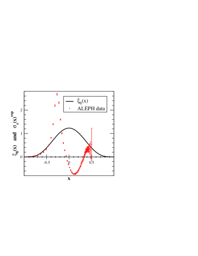
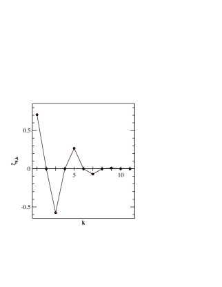
Figure 1: Distribution $\xi_{a}(x)$ for $a=8$. Its corresponding components $\xi_{a,k}$ are shown on the right-hand-side. The distribution is shown together with the reference data $\sigma_{z}^{{}^{LR}}(x)^{exp}$ [22] for $z=1$ GeV².

Since $\xi_{a}(x)$ is a polynomial of degree $a$, it accepts a decomposition in terms of the orthonormal basis of Legendre polynomial $\left\{g_{k}(x)\right\}_{k=1}^{\infty}$:

$$\xi_{a}(x)\,\,=\,\,\sum_{k=1}^{a+1}\,\xi_{a,k}\,\,\,g_{k}(x)\,,$$ (17)

where $\xi_{a,1}=1/\sqrt{2}$ due to the normalization $\displaystyle{\int}_{-1}^{1}dx\,\,\,\xi_{a}(x)=1$, and the constant terms $\xi_{a,k}$ with even $k$ are zero due to the parity of $\xi_{a}(x)$. This distribution only depends on the first $a+1$ Legendre polynomials. In Fig. (1) we show the distribution and components of $\xi_{8}(x)$, compared to the experimental data $\sigma_{z}^{{}^{LR}}(x)^{exp}$ for $z=1$ GeV² [22]. For the case with $a=8$ we have $\xi_{8,3}=-\frac{2\sqrt{10}}{11},\,\xi_{8,5}=\frac{27\sqrt{2}}{143},\,\xi_{8,7}=-\frac{2\sqrt{26}}{143}$ and ${\xi_{8,9}=\frac{7\sqrt{34}}{4862}}$.

The mean value of the spectral function is defined through the average

$$\frac{\displaystyle 1}{\displaystyle\pi}\mbox{Im}\overline{\Pi}(z)^{{}^{\xi_{a}}}\,\,\equiv\,\,\langle\,\sigma_{z}\,\rangle_{\xi_{a}}\,\,=\,\,\displaystyle{\int}_{-1}^{1}\,dx\,\,\sigma_{z}(x)\,\,\xi_{a}(x)\,\,,$$ (18)

where the orthonormal decomposition of the correlator in Eq. (11) yields

$$\frac{\displaystyle 1}{\displaystyle\pi}\mbox{Im}\overline{\Pi}(z)^{{}^{\xi_{a}}}\,\,=\,\,\sum_{k=1}^{a+1}\,\xi_{a,k}\,\,\,\mathcal{B}^{{}^{(k)}}(z)\,\,\,.$$ (19)

Only the first $(a+1)$ moments are relevant for the amplitude averaged through $\xi_{a}$. This will be useful when our control on the high order components is reduced.

This procedure is analogous to the Gauss-Weirstrass transform of the correlator, where the amplitude is averaged through a Gaussian distribution [19]. One would recover Im$\overline{\Pi}(z)^{{}^{\xi_{a}}}\to$Im$\Pi(z)$ in the limit when $a\to\infty$. Nonetheless, our theoretical control on the QCD components $\mathcal{B}^{{}^{(k)}}(z)$ gets worse as $k$ increases and one needs to go to high enough energies in order to make them reliable.

3 Perturbative QCD and the operator product expansion

The Operator Product Expansion in perturbative QCD provides a systematic procedure to compute the two-point Green functions at any order in $\alpha_{s}$ or operator dimension in the deep euclidean regime $Q^{2}\equiv-q^{2}\gg\Lambda_{{}_{QCD}}^{2}$ [3, 5]. For the spin–1 correlators one has

$$\Pi(-Q^{2})^{{}^{OPE}}\,\,=\,\,\,\,\,\,\langle\,{{\cal O}}_{{}_{(0)}}\,\rangle\,\,\,\,+\,\,\,\,\sum_{m=2}^{\infty}\,\,\frac{\displaystyle\langle\,{{\cal O}}_{{}_{(2m)}}\,\rangle}{\displaystyle Q^{2m}}\,\,,$$ (20)

where the coefficients $\langle\,{\cal O}_{(2m)}\,\rangle$ are provided by the dimension–$(2m)$ operator in the OPE and they depend weakly on the momenta (only through logarithms) [5]. In this work, the term $\langle\,{\cal O}_{{}_{(0)}}\,\rangle$ corresponds to the identity operator in the OPE and yields the purely perturbative QCD contribution (pQCD). The $V+A$ correlator becomes ${\langle\,{\cal O}^{{}^{LL}}_{{}_{(0)}}\,\rangle\stackrel{{\scriptstyle\alpha_{s}\to 0}}{{\longrightarrow}}\Pi_{{}_{LL}}(-Q^{2})^{{}^{free}}=-\frac{N_{C}}{12\pi^{2}}\ln{\frac{Q^{2}}{\mu^{2}}}}$ in the free quark limit whereas for the $V-A$ Green function vanishes for any value of $\alpha_{s}$ (${\langle\,{\cal O}^{{}^{LR}}_{{}_{(0)}}\,\rangle=\Pi_{{}_{LR}}(-Q^{2})^{free}=0}$).

V-A correlator
     In the case of the $V-A$ correlator ($\Pi_{{}_{LR}}=\Pi_{{}_{VV}}-\Pi_{{}_{AA}}$) the OPE starts at the dimension six operator [5]:

$$\Pi_{{}_{LR}}(-Q^{2})^{{}^{OPE}}\,\,\,=\,\,\,\,\,\,\sum_{m=3}^{\infty}\frac{\displaystyle\langle\,{\cal O}_{{}_{(2m)}}^{{}^{LR}}\,\rangle}{\displaystyle Q^{2m}}\,.$$ (21)

At  high   euclidean  momenta   the  correlator   is  driven   by   the  dimension   six   condensate,  with ${\langle\,{\cal O}_{{}_{(6)}}^{{}^{LR}}\,\rangle=\,-4\pi\alpha_{s}\langle\,\bar{q}q\,\rangle^{2}}$ at large $N_{C}$. We will not consider the anomalous dimensions of the condensates $\langle\,{\cal O}_{{}_{(2m)}}\,\rangle$, which will be taken as constants. In this case, one gets for the moments a $1/Q^{2m}$ power structure,

$$\mathcal{A}_{{}_{LR}}^{{}^{(n)}}(Q^{2})^{{}^{OPE}}\,\,\,=\,\,\,\,\,\,\,\,\,\,\sum_{m=3}^{\infty}\,\frac{\displaystyle a^{{}^{LR}}_{{}_{(n,2m)}}}{\displaystyle Q^{2m}}\,,\qquad\mbox{ with }\quad a^{{}^{LR}}_{{}_{(n,2m)}}\,=\,\frac{\displaystyle(m-1+n)!}{\displaystyle(m-1)!\,\,n!}\,\,\langle\,{\cal O}_{(2m)}^{{}^{LR}}\,\rangle\,,$$ (22)

and a similar thing happens for the components $\mathcal{B}^{{}^{(k)}}(Q^{2})$,

$$\mathcal{B}_{{}_{LR}}^{{}^{(k)}}(Q^{2})^{{}^{OPE}}\,\,\,\,=\,\,\,\,\,\,\,\,\sum_{m=3}^{\infty}\,\frac{\displaystyle b_{{}_{(k,2m)}}^{{}^{LR}}}{\displaystyle Q^{2m}}\,,\qquad\mbox{ with }\quad b_{{}_{(k,2m)}}\,=\,\sum_{n=1}^{k}\,M^{{}^{\mathcal{B}\mathcal{A}}}_{k,n}\,\,\,a_{{}_{(n,2m)}}^{{}^{LR}}\,,$$ (23)

being the constants $M^{{}^{\mathcal{B}\mathcal{A}}}_{k,n}$ given by the basis transformation in Eq. (12) that relates $\mathcal{A}^{{}^{(n)}}(Q^{2})$ and $\mathcal{B}^{{}^{(k)}}(Q^{2})$. When considering truncated OPE series, both $\mathcal{A}^{{}^{(n)}}_{{}_{LR}}(Q^{2})$ and $\mathcal{B}^{{}^{(n)}}_{{}_{LR}}(Q^{2})$ diverge beyond some order $n$.

The spectral function, related to the components $\mathcal{B}^{{}^{(k)}}(Q^{2})$ through Eq. (15), formally shows the same power behaviour,

$$\frac{\displaystyle 1}{\displaystyle\pi}\mbox{Im}\Pi_{{}_{LR}}(z)\,\,\,=\,\,\,\displaystyle{\sum_{m=3}^{\infty}}\,\frac{\displaystyle\frac{1}{\pi}\mbox{Im}\Pi^{{}^{LR}}_{{}_{(2m)}}}{\displaystyle z^{m}}\,,\qquad\mbox{ with }\quad\frac{1}{\pi}\mbox{Im}\Pi^{{}^{LR}}_{{}_{(2m)}}\,=\,\displaystyle{\sum_{k=1}^{\infty}}\,b_{{}_{(k,2m)}}^{{}^{LR}}\,\cdot\,g_{k}(0)\,.$$ (24)

Unfortunately, within the OPE the terms $b_{{}_{(k,2m)}}$ in the coefficients $\frac{1}{\pi}\mbox{Im}\Pi^{{}^{LR}}_{{}_{(2m)}}$ go on growing as $k\to\infty$ and the summation diverges, preventing the theoretical determination of the spectral function.

V+A correlator
     Considering  the   Renormalization  Group   Equations  up   to  ${\cal O}(\alpha_{s})$,  the  $V+A$  correlator  (${\Pi_{{}_{LL}}=\Pi_{{}_{VV}}+\Pi_{{}_{AA}}}$) shows the structure [5]

$$\Pi_{{}_{LL}}(-Q^{2})^{{}^{OPE}}\,\,\,\,=-\,\frac{\displaystyle N_{C}}{\displaystyle 12\pi^{2}}\,\left[\,\ln{\frac{\displaystyle Q^{2}}{\displaystyle\mu^{2}}}\,\,\,-\,\,\,\frac{\displaystyle 3C_{F}}{\displaystyle 2\beta_{1}}\,\ln{\left(\frac{\displaystyle\alpha_{s}(\mu^{2})}{\displaystyle\alpha_{s}(Q^{2})}\right)}\,\right]\,\,\,\,+\,\,\,\sum_{m=2}^{\infty}\frac{\displaystyle\langle\,{\cal O}_{(2m)}^{{}^{LL}}\,\rangle}{\displaystyle Q^{2m}}\,,$$ (25)

with $C_{F}=\frac{N_{C}^{2}-1}{2\,N_{C}}$, and     $\beta_{1}=-\frac{1}{6}(11\,N_{C}-2\,n_{f})$    provided    by     the      $\beta$–function       at     lowest     order,      $\frac{d\ln{\alpha_{s}}}{d\ln{\mu}}=\beta(\alpha_{s})=\frac{1}{\pi}\beta_{1}\alpha_{s}+{\cal O}(\alpha_{s}^{2})$, being $\alpha_{s}(\mu^{2})$ the strong running coupling constant.

For pQCD, with all the condensates set to zero, one finds the moments

$$\mathcal{A}_{{}_{LL}}^{{}^{(n)}}(Q^{2})^{{}^{pQCD}}\,\,\,\,=\,\,\,\,\frac{\displaystyle 1}{\displaystyle n}\,\frac{\displaystyle N_{C}}{\displaystyle 12\pi^{2}}\,\left(1\,+\,\frac{\displaystyle 3C_{F}}{\displaystyle 4}\,\frac{\displaystyle\alpha_{s}(Q^{2})}{\displaystyle\pi}\right)\,\,\,\,+\,\,\,{\cal O}(\alpha_{s}^{2}(Q^{2}))\,,$$ (26)

which provides the components

$$\mathcal{B}_{{}_{LL}}^{{}^{(k)}}(Q^{2})^{{}^{pQCD}}\,\,\,\,=\,\,\,\,\sqrt{2}\,\frac{\displaystyle N_{C}}{\displaystyle 12\pi^{2}}\,\left(1\,+\,\frac{\displaystyle 3C_{F}}{\displaystyle 4}\,\frac{\displaystyle\alpha_{s}(Q^{2})}{\displaystyle\pi}\right)\,\,\delta^{k,1}\,\,\,\,+\,\,\,{\cal O}(\alpha_{s}^{2}(Q^{2}))\,.$$ (27)

The perturbative expansion of pQCD in powers of $\alpha_{s}$ produces the spectral function

$$\frac{\displaystyle 1}{\displaystyle\pi}\mbox{Im}\Pi_{{}_{LL}}(z)^{{}^{pQCD}}\,\,\,\,=\,\,\,\,\sum_{k=1}^{\infty}\,\mathcal{B}^{{}^{(k)}}(z)^{{}^{pQCD}}\,\cdot\,g_{k}(0)\,\,\,\,=\,\,\,\,\frac{\displaystyle N_{C}}{\displaystyle 12\pi^{2}}\,\left(1\,+\,\frac{\displaystyle 3C_{F}}{\displaystyle 4}\,\frac{\displaystyle\alpha_{s}(z)}{\displaystyle\pi}\right)\,\,\,\,+\,\,\,{\cal O}(\alpha_{s}^{2}(z))\,.$$ (28)

Nevertheless, once the higher dimension operators are taken into account ($\langle\,{\cal O}_{(4)}^{{}^{LL}}\,\rangle=\frac{1}{12\pi}\alpha_{s}\langle\,G_{\mu\nu}^{a}G^{\mu\nu}_{a}\,\rangle$, $\langle\,{\cal O}_{(6)}^{{}^{LL}}\,\rangle=\frac{8}{9}\pi\alpha_{s}\langle\,\bar{q}q\,\rangle^{2},...$) the series of $\mathcal{B}^{{}^{(k)}}_{{}_{LL}}(z)$ becomes divergent when $k\to\infty$, as it happened before in the $V-A$ case.

3.1 Divergence of the components $\mathcal{B}^{{}^{(k)}}(Q^{2})$ within the OPE framework

Since the moments of the truncated OPE amplitudes diverge at some point, it is important to study how and when this divergence occurs. Since we are now interested on dealing with finite spectral functions, the pion pole is removed from the correlators for the analysis in this section:

$$\Pi_{{}_{LR}}(-Q^{2})^{{}^{no-\pi}}\,\,\,\equiv\,\,\,\left[\Pi_{{}_{LR}}(-Q^{2})\,+\,\frac{\displaystyle F^{2}}{\displaystyle Q^{2}}\right]\quad,\qquad\qquad\Pi_{{}_{LL}}(-Q^{2})^{{}^{no-\pi}}\,\,\,\equiv\,\,\,\left[\Pi_{{}_{LL}}(-Q^{2})\,-\,\frac{\displaystyle F^{2}}{\displaystyle Q^{2}}\right]\,,$$ (29)

which yields the moments

$$\mathcal{A}^{{}^{(n)}}_{{}_{LR}}(Q^{2})_{{}_{no-\pi}}=\left[\mathcal{A}_{{}_{LR}}^{{}^{(n)}}(Q^{2})+\frac{\displaystyle F^{2}}{\displaystyle Q^{2}}\right]\quad,\qquad\qquad\mathcal{A}^{{}^{(n)}}_{{}_{LL}}(Q^{2})_{{}_{no-\pi}}=\left[\mathcal{A}_{{}_{LL}}^{{}^{(n)}}(Q^{2})-\frac{\displaystyle F^{2}}{\displaystyle Q^{2}}\right]\,,$$ (30)

with $F\simeq F_{\pi}=0.0924$ MeV. This allows working with squared integrable spectral functions $\sigma_{z}(x)^{{}^{no-\pi}}$, owning a convergent series of components $\mathcal{B}^{{}^{(k)}}(z)_{{}_{no-\pi}}$.

In order to estimate the physical components $\mathcal{B}^{{}^{(k)}}(Q^{2})_{{}_{no-\pi}}$, we show in Figs. (2) and (3) the components obtained from the experimental ansatz,

$$\mbox{Im}\Pi(t)^{{}^{ansatz}}_{{}_{no-\pi}}\,\,\,\,=\,\,\,\,\mbox{Im}\Pi(t)^{{}^{exp}}_{{}_{no-\pi}}\,\cdot\,\theta(t_{0}-t)\,\,\,+\,\,\,\mbox{Im}\Pi(q^{2})^{{}^{pQCD}}\,\cdot\,\theta(t-t_{0})\,\,,$$ (31)

being Im$\Pi(t)^{{}^{exp}}_{{}_{no-\pi}}$ the experimental data with the pion pole removed [22] and $t_{0}=3$ GeV². In order to recover global duality one cannot take an arbitrary matching point [19, 38], though the duality becomes better and better as $t_{0}$ is increased and the oscillations in the spectral function vanish. Although the experimental data only reach up to $t=M_{\tau}^{2}$ in the $\tau$–decay experiments [22, 23, 24], one knows from the $e^{+}e^{-}$ experiments that pQCD provides an appropriate description of the vector spectral function [2]. Even the $\tau$ data for the $V+A$ correlator already show this regularity for $t\mathrel{\hbox to0.0pt{\lower 4.0pt\hbox{\hskip 1.0pt$\sim$}\hss}\raise 1.0pt\hbox{$>$}}2$ GeV². Our experimental ansatz is however less accurate in the $V-A$ channel where the fluctuations are wider than in $\frac{1}{\pi}$Im$\Pi_{{}_{LL}}(t)$ and they still remain sizable at the $\tau$–threshold. Nonetheless, for $Q^{2}\sim t_{0}$, the $\mathcal{B}^{{}^{(k)}}(Q^{2})$ sum rules suppress the transition region $t\sim t_{0}$ as $k$ grows, providing this ansatz a first estimate of the physical components.

We can see in Fig. (2) that, although the leading order OPE contribution governs the very first components, these eventually diverge. We have taken the value ${\langle\,{\cal O}_{{}_{(6)}}^{{}^{LR}}\,\rangle\simeq-3.8\cdot 10^{-3}}$ GeV⁶ in order to illustrate the behaviour of the $\mathcal{B}_{{}_{LR}}^{{}^{(k)}}(Q^{2})_{{}_{no-\pi}}$ [8]. Adding the contribution from some higher dimension operators does not solve the problem of the convergence at low energies ($Q^{2}=2$ GeV²), as one can see in the first plot of Fig. (2). We have used the values $\langle\,{\cal O}_{(8)}^{{}^{LR}}\,\rangle\simeq 6.0\cdot 10^{-3}$ GeV⁸, $\langle\,{\cal O}_{(10)}^{{}^{LR}}\,\rangle\simeq-9.1\cdot 10^{-3}$ GeV¹⁰, $\langle\,{\cal O}_{(12)}^{{}^{LR}}\,\rangle\simeq 11.9\cdot 10^{-3}$ GeV¹² from the review in Ref. [8], although there is still some controversy about the value of the higher dimension condensates [6, 8, 9, 10].
     However, the situation improves drastically once we go to the deep euclidean regime. At $Q^{2}=10$ GeV² (second plot in Fig. (2)), the addition of higher dimension contributions produces appreciable improvements in the convergence of the $\mathcal{B}_{{}_{LR}}^{{}^{(k)}}(Q^{2})_{{}_{no-\pi}}$. In Fig. (2) and next figures, all the plots are normalized such that $\frac{1}{\pi}$Im$\Pi_{{}_{LL}}(t)^{{}^{pQCD}}\stackrel{{\scriptstyle t\to\infty}}{{\longrightarrow}}1$.

A  similar   result  is  obtained  for   the  $V+A$   correlator,  where   the  inclusion  of higher dimension operators  improves  slightly the description  in the deep euclidean region   ($Q^{2}=10$ GeV², second plot  in   Fig. (3)).  We   have   considered   the  chiral  limit  and   used   the  values   $\alpha_{s}(Q^{2})=-2\pi/\left[\beta_{1}\ln{(Q^{2}/\Lambda_{{}_{QCD}}^{2})}\right]$,    with $\Lambda_{{}_{QCD}}\simeq 0.235$ GeV  and  $n_{f}=3$ [2],    ${\langle\,{\cal O}_{{}_{(4)}}^{{}^{LL}}\,\rangle=\frac{1}{12\pi}\alpha_{s}\langle\,G_{\mu\nu}^{a}G^{\mu\nu}_{a}\,\rangle\simeq 1.2\cdot 10^{-3}}$ [11], ${\langle\,{\cal O}_{{}_{(6)}}^{{}^{LL}}\,\rangle=\frac{8\pi}{9}\alpha_{s}\langle\,\bar{q}q\,\rangle^{2}\simeq 0.85\cdot 10^{-3}}$ [8].

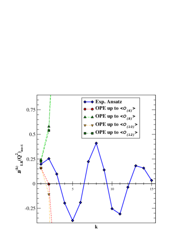
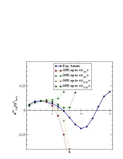
Figure 2: Components $\mathcal{B}_{{}_{LR}}^{{}^{(k)}}(Q^{2})_{{}_{no-\pi}}$ for the $V-A$ correlators provided by the OPE at $Q^{2}=2$ GeV² and $Q^{2}=10$ GeV² (left and right-hand-side, respectively). It is compared to the components derived from the experimental ansatz. From now on, the amplitudes in the plots are normalized such that $\frac{1}{\pi}$Im$\Pi_{{}_{LL}}(t)^{{}^{pQCD}}\stackrel{{\scriptstyle t\to\infty}}{{\longrightarrow}}1$.

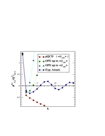
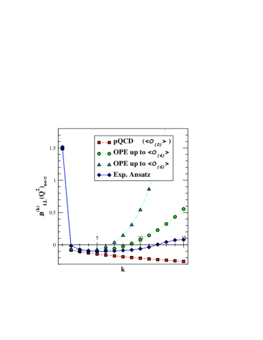
Figure 3: Components $\mathcal{B}_{{}_{LL}}^{{}^{(k)}}(Q^{2})_{{}_{no-\pi}}$ for the $V+A$ correlators provided by the OPE at $Q^{2}=2$ GeV² and $Q^{2}=10$ GeV².

3.2 Averaged correlators within the OPE

We have seen that the OPE remains reliable only up to a given finite order $k$ in the moments. Through the consideration of a convenient distribution function $\xi_{a}(x)$, we can nevertheless remove the influence of the components $\mathcal{B}^{{}^{(k)}}(Q^{2})$ of order $k>a+1$. The averaged OPE amplitude is obtained from the calculation of the moments in the euclidean domain and it is compared to the averaged amplitude coming from the experimental ansatz in the minkowskian region.

The transform of the $1/Q^{2m}$ terms, e.g. in the $V-A$ correlator, produces again an OPE-like power series:

$$\Pi_{{}_{LR}}(-Q^{2})\,=\,\sum_{m=3}^{\infty}\frac{\displaystyle\langle\,{\cal O}^{{}^{LR}}_{{}_{(2m)}}\,\rangle}{\displaystyle Q^{2m}}\qquad\longrightarrow\qquad\frac{\displaystyle 1}{\displaystyle\pi}\mbox{Im}\overline{\Pi}_{{}_{LR}}(z)^{{}^{\xi_{a}}}\,=\,\sum_{m=\frac{a}{2}+1}^{\infty}\frac{\displaystyle\frac{1}{\pi}\mbox{Im}\overline{\Pi}^{{}^{LR,\,\xi_{a}}}_{{}_{(2m)}}}{\displaystyle z^{m}}\,\,,$$ (32)

with the coefficients $\frac{1}{\pi}$Im$\overline{\Pi}^{{}^{LR,\,\xi_{a}}}_{{}_{(2m)}}\,=\,(-1)^{\frac{a}{2}}\,\,\langle\,{\cal O}^{{}^{LR}}_{{}_{(2m)}}\,\rangle\,\,\,\,\left[\frac{2^{a+1}\,\,\Gamma\left(\frac{a}{2}+\frac{3}{2}\right)}{\sqrt{\pi}\,\Gamma(a+2)\,\Gamma\left(\frac{a}{2}+1\right)}\,\,\frac{\Gamma\left(m+\frac{a}{2}+1\right)}{\Gamma\left(m-\frac{a}{2}\right)}\right]$, and where the condensates $\langle\,{\cal O}_{{}_{(2m)}}^{{}^{LR}}\,\rangle$ have been taken as a constant.

For a given $\xi_{a}(x)$, the average of a rational term $\Pi(-Q^{2})\sim\frac{\displaystyle\langle\,{\cal O}_{{}_{(2m)}}\,\rangle}{\displaystyle Q^{2m}}$ is then zero whenever $2m\leq a$, so the averaged amplitude is never sensitive to the presence of the pion pole. This means that, in the short distance region where the ${V-A}$ correlator is expected to be governed by the $\frac{\displaystyle\langle\,{\cal O}^{{}^{LR}}_{{}_{(6)}}\,\rangle}{\displaystyle Q^{6}}$ term, the averaged spectral function is zero for $a\geq 6$. Likewise, $\frac{1}{\pi}$Im$\overline{\Pi}_{{}_{LR}}(z)^{{}^{\xi_{a}}}$ accepts the same number of Weinberg sum-rules as the original amplitude $\frac{1}{\pi}$Im$\Pi_{{}_{LR}}(t)$. Its non-zero experimental value for $\xi_{8}(x)$ (first plot in Fig. (4)) hints that for $z\mathrel{\hbox to0.0pt{\lower 4.0pt\hbox{\hskip 1.0pt$\sim$}\hss}\raise 1.0pt\hbox{$<$}}5$ GeV² the corrections from $\langle\,{\cal O}_{{}_{(2m)}}\,\rangle$ with $m\geq 5$ produce rather relevant effects.

In $\Pi_{{}_{LL}}(-Q^{2})^{{}^{pQCD}}$ up to ${\cal O}(\alpha_{s})$, one finds from Eqs. (27) and (28) that for any $\xi_{a}(x)$,

$$\frac{\displaystyle 1}{\displaystyle\pi}\mbox{Im}\overline{\Pi}_{{}_{LL}}(q^{2})^{{}^{pQCD}}\,\,\,\,=\,\,\,\,\left.\frac{\displaystyle 1}{\displaystyle\pi}\mbox{Im}\Pi_{{}_{LL}}(q^{2})^{{}^{pQCD}}\right|_{{}_{{\cal O}(\alpha_{s})}}\,\,\,\,+\,\,\,\,{\cal O}(\alpha_{s}^{2})\,\,.$$ (33)

It would be interesting to study how this identity is modified at higher orders in $\alpha_{s}$. The comparison of the theoretical $V+A$ averaged correlator to our experimental ansatz is provided on the second plot from Fig. (4), showing a very good agreement within ${\cal O}(\alpha_{s}^{2})$ uncertainties –solid band–. For $\xi_{8}(x)$, the average is independent of $\langle\,{\cal O}_{{}_{(4)}}^{{}^{LL}}\,\rangle$, $\langle\,{\cal O}_{{}_{(6)}}^{{}^{LL}}\,\rangle$ and $\langle\,{\cal O}_{{}_{(8)}}^{{}^{LL}}\,\rangle$, being governed by the pQCD distribution. On the contrary to $\Pi_{{}_{LR}}(-Q^{2})$, the contributions from the condensates $\langle\,{\cal O}_{{}_{(2m)}}^{{}^{LL}}\,\rangle$ with $m\geq 5$ seem to be much more suppressed.

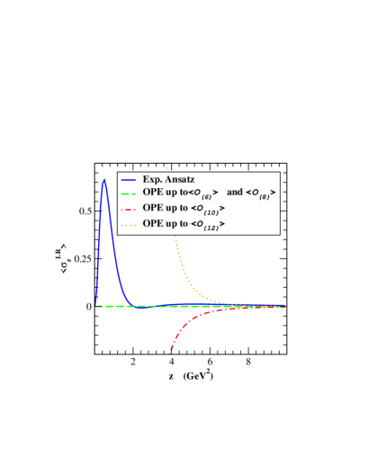
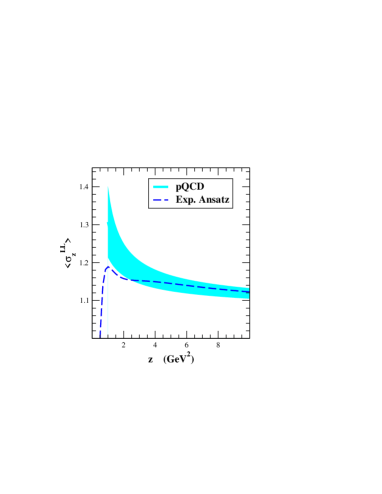
Figure 4: $V-A$ and $V+A$ correlators $\sigma_{z}(x)$ averaged by the distribution $\xi_{8}(x)$ (${\langle\,\sigma_{z}\,\rangle_{{}_{\xi_{8}}}=\frac{1}{\pi}\mbox{Im}\overline{\Pi}(z)^{{}^{\xi_{8}}}}$). The solid band on the second plot represents the ${\cal O}(\alpha_{s}^{2})$ uncertainties.

By considering appropriate distributions $\xi_{a}(x)$ one has, in addition, the possibility of recovering $\alpha_{s}$ and the vector condensates $\langle\,{\cal O}_{{}_{(2m)}}^{{}^{VV}}\,\rangle$ through a direct analysis of the $e^{+}e^{-}$ experimental measurements [26, 27]. Nonetheless, this analysis escapes the aim of this article and it is left for a next work. The situation in the $V-A$ case seems not so favourable since the energy range of data is much more reduced ($t\leq M_{\tau}^{2}\simeq 3$ GeV²), mainly laying within the long distance region where the OPE stops being valid.

4 QCD correlators in resonance theory at large $N_{C}$

In order to inspect the range of energies where the OPE breaks down it is necessary to add some extra ingredients to our theory. One has to add a mechanism that fully reproduces the OPE expressions at high euclidean momenta, being able, in addition, to provide the right low energy theory ($\chi PT$) and the minkowskian description (experimental data, resonance structure…). We will see how a theory with explicit resonances suits this picture.

The exact recovering of perturbative QCD requires the full pile of hadronic states. However, the infinite summation of resonance from large $N_{C}$ QCD is by itself a limit. One of the available methods to regularise the series is through an ultraviolet cut-off. Hence, one constructs a set of quantum field theories, $R\chi T^{(n)}$, with a finite number $n$ of resonances to describe the observables at some given momentum $p^{\mu}$ [35, 36, 37]. $QCD_{\infty}$ would be recovered by taking the limit $n\to\infty$ keeping the external momenta fixed ($R\chi T^{(n)}[p^{\mu}]\stackrel{{\scriptstyle n\to\infty}}{{\longrightarrow}}R\chi T^{(\infty)}[p^{\mu}]=QCD_{\infty}[p^{\mu}]$).

Accommodating $R\chi T^{(\infty)}$ and QCD at large $N_{C}$ is not trivial. The first approach must be focused on recovering pQCD in the deep euclidean domain. The appearance at $N_{C}\to\infty$ of non-perturbative condensates in the OPE produces small corrections into the pQCD correlator at $Q^{2}\gg\Lambda_{{}_{QCD}}^{2}$. However, due to the non-perturbative effects at large $N_{C}$, the smooth pQCD spectral function turns into a meromorphic function with an infinite number of real poles.

It is important to recall the possible existence of duality violating terms. The Green-functions $\langle\,T\{J_{\mu}(x)J^{\dagger}_{\nu}(0)\}\,\rangle$ are not fully determined by the singularities at $x^{2}=0$ [20]. For instance, one may have terms of the form $\frac{1}{x^{2}+\rho^{2}}$, whose Fourier transform falls off in the deep euclidean as $\exp{\left(-Q\,\rho\right)}$ but becomes oscillating, $\sin{\left(q\,\rho\right)}$, in the minkowskian region ($Q\equiv\sqrt{-q^{2}}$ and $q\equiv\sqrt{q^{2}}$). It is actually interesting that some resonance models generate explicitly this kind of duality violating terms [31, 32], pointing out the fact that a resonance theory is fully able to produce both the OPE and non-OPE QCD singularities. We will derive the OPE condensates in this section by neglecting the duality violating terms in the deep euclidean domain although further works should focus on the estimate of these terms [21].

In real world, the resonance poles become complex and get shifted to unphysical Riemann sheets due to Dyson-Schwinger resummations at all orders in $1/N_{C}$; once the higher $1/N_{C}$ corrections are taken into account and the resonance gain their physical non-zero widths the amplitude becomes again smooth, as it is found experimentally. The width can be accurately computed in some situations [57, 58, 61], although its derivation is, in general, non-trivial.

4.1 $V+A$ correlator in resonance theory

At large $N_{C}$, the spin–1 correlators are meromorphic functions characterised by the position and residues of their poles. The $V+A$ spectral function is given by

$$\frac{\displaystyle 1}{\displaystyle\pi}\mbox{Im}\Pi_{{}_{LL}}(t)^{{}^{N_{C}\to\infty}}\,\,=\,\,\,\,F^{2}\,\delta(t)\,\,+\,\,\displaystyle{\lim_{M_{\infty}^{2}\to\infty}}\,\,\,\displaystyle{\sum_{M_{j}^{2}\leq M_{\infty}^{2}}}\,F_{j}^{2}\,\,\,\delta(t-M_{j}^{2})\,,$$ (34)

which generates the moment integrals given by the positive meromorphic functions

$$\begin{array}[]{rl}\mathcal{A}^{{}^{(n)}}_{{}_{LL}}(Q^{2})^{{}^{N_{C}\to\infty}}\,\,=&\,\,\,\,\frac{\displaystyle F^{2}}{\displaystyle Q^{2}}\,\,+\,\,\displaystyle{\lim_{M_{\infty}^{2}\to\infty}}\,\,\,\displaystyle{\sum_{M_{j}^{2}\leq M_{\infty}^{2}}}\,\frac{\displaystyle F_{j}^{2}\,Q^{2n}}{\displaystyle(M_{j}^{2}+Q^{2})^{n+1}}\,,\end{array}$$ (35)

with $M_{\infty}$ denoting the mass of the highest resonance in the resonance theory. the constants $M_{j}$ and $F_{j}$ are the mass and coupling constant of the vector and axial-vector states at LO in $1/N_{C}$ and $F$ is the pion decay constant. In the limit when $M_{\infty}^{2}\to\infty$, this upper mass acts like an ultraviolet cut-off of the large $N_{C}$ infinite resonance summation [30, 35, 36, 37]. Taking the $Q^{2}\to\infty$ limit is not trivial at all since there is always an infinite set of resonance above any considered $Q^{2}$, whose effects are in general not so clearly negligible. From now on, the limit $M_{\infty}^{2}\to\infty$ will be always implicitly assumed.

4.1.1 Perturbative and non-perturbative contributions in pQCD

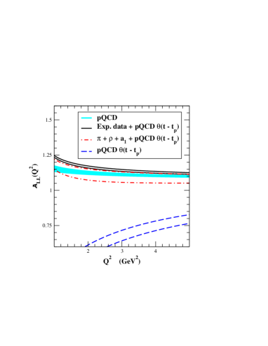
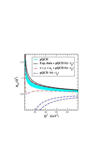
Figure 5: $V+A$ Adler function from the pQCD space-like calculation up to ${\cal O}(\alpha_{s})$, where the band represents the ${\cal O}\left(\alpha_{s}^{2}\right)$ uncertainties. It is compared with $\mathcal{A}_{{}_{LL}}(Q^{2})_{{}_{pert.}}^{{}^{pQCD}}$, derived through dispersion relations from considering the spectral function $\frac{1}{\pi}$Im$\Pi_{{}_{LL}}(t)^{{}^{pQCD}}\,\cdot\,\theta(t-t_{p})$ (dashed curve, ${t_{p}=(1.25}$ GeV$)^{2}$ and $t_{p}=(1.45$ GeV$)^{2}$ for the upper an lower curves respectively). The dashed–dotted curve includes also the contributions from the pion, $\rho(770)$ and $a_{1}(1260)$ whereas the solid lines consider instead the experimental data [22] for the spectral function at $t<t_{p}$.

In this section we make an analysis of pQCD which will be relevant for the resonance calculation. We study how the pQCD amplitude is recovered in the deep euclidean thanks to a spectral function that behaves like $\frac{1}{\pi}$Im$\Pi_{{}_{LL}}(t)^{{}^{pQCD}}$ at high energies.

We will consider an auxiliary spectral function with the form

$$\frac{\displaystyle 1}{\displaystyle\pi}\mbox{Im}\Pi_{{}_{LL}}(t)^{{}^{pQCD}}_{{}_{pert.}}\,\,\,\,\equiv\,\,\,\,\frac{\displaystyle 1}{\displaystyle\pi}\mbox{Im}\Pi_{{}_{LL}}(t)^{{}^{pQCD}}\,\,\cdot\,\,\theta(t-t_{p})\,\,,$$ (36)

where the low energy region has been removed. It yields the moments

$$\mathcal{A}_{{}_{LL}}^{{}^{(n)}}(Q^{2})^{{}^{pQCD}}_{{}_{pert.}}\,\,\,\,=\,\,\,\,\displaystyle{\int}_{t_{p}}^{\infty}\,\,\frac{\displaystyle dt\,\,Q^{2n}}{\displaystyle(t+Q^{2})^{n+1}}\,\,\frac{\displaystyle 1}{\displaystyle\pi}\mbox{Im}\Pi_{{}_{LL}}(t)^{{}^{pQCD}}\,\,.$$ (37)

In the deep euclidean, these moment integrals recover the pQCD moments $\mathcal{A}_{{}_{LL}}^{{}^{(n)}}(Q^{2})^{{}^{pQCD}}$ with the proper $\alpha_{s}$ running up to subdominant $1/Q^{2m}$ power corrections.

The corresponding Adler function up to ${\cal O}(\alpha_{s})$ is plotted in Fig. (5). The solid band covers an uncertainty of $\pm(\frac{\alpha_{s}}{\pi})^{2}$. The value of $t_{p}$ was varied between the values $t_{p}=(1.26$ GeV$)^{2}$ and $t_{p}=(1.45$ GeV$)^{2}$. However, the asymptotic behaviour $\mathcal{A}_{{}_{LL}}(Q^{2})^{{}^{pQCD}}_{{}_{pert}}=\left.\mathcal{A}_{{}_{LL}}(Q^{2})^{{}^{pQCD}}\right|_{{}_{{\cal O}(\alpha_{s})}}+{\cal O}(\alpha_{s}^{2})$ is only achieved at energies $Q^{2}\gg 100$ GeV², by far much larger than the expected $Q^{2}\sim 2$ GeV². These discrepancies are much easier to understand through the observance of the Adler function at ${\cal O}(\alpha_{s}^{0})$:

$$\mathcal{A}_{{}_{LL}}(Q^{2})^{{}^{pQCD}}_{{}_{pert.}}=\frac{\displaystyle N_{C}}{\displaystyle 12\pi^{2}}\left[\frac{\displaystyle Q^{2}}{\displaystyle Q^{2}+t_{p}}\right]+{\cal O}(\alpha_{s})=\frac{\displaystyle N_{C}}{\displaystyle 12\pi^{2}}\left[\,1\,\,-\,\,\frac{\displaystyle t_{p}}{\displaystyle Q^{2}}\,\,\,+\,\,\,{\cal O}\left(\frac{\displaystyle t_{p}^{2}}{\displaystyle Q^{4}}\right)+{\cal O}(\alpha_{s})\right]\,,$$ (38)

where the $\frac{\displaystyle t_{p}}{\displaystyle Q^{2}}$ term generates deviations of the order of 1% at $Q^{2}=100$ GeV², larger than those coming from the ${\cal O}(\alpha_{s}^{2})$ corrections.

This points out that although the high energy logarithmic dependence of Im$\Pi_{{}_{LL}}(t)^{{}^{pQCD}}_{{}_{pert.}}$ provides the proper asymptotic behaviour of the pQCD moment integrals, the non-perturbative region owns crucial information about how fast this limit is reached. If one includes the contribution of the resonances laying on $t<t_{p}$ (Goldstones from the chiral symmetry breaking, $\rho(770)$ and $a_{1}(1260)$) the asymptotic behaviour is again reached within the expected range of energies. Alternatively, one may consider the experimental data for Im$\Pi_{{}_{LL}}(t)$ at $t<t_{p}$ [22], getting similar results due to the moderate size of the width of these states ($M_{j}\Gamma_{j}\mathrel{\hbox to0.0pt{\lower 4.0pt\hbox{\hskip 1.0pt$\sim$}\hss}\raise 1.0pt\hbox{$<$}}\frac{\displaystyle 1}{\displaystyle N_{C}}\,\cdot\,M_{j}^{2}$). For Fig. (5) we have use the inputs $M_{\rho}=0.77$ GeV, $M_{a_{1}}=1.26$ GeV, $F=92.4$ MeV, $F_{\rho}=154$ MeV and $F_{a_{1}}=123$ MeV [41, 65].

4.1.2 Perturbative and non-perturbative contributions in $QCD_{\infty}$

We analyse in this section the conditions to recover pQCD in the deep euclidean region of momenta through a resonance theory. pQCD will naturally arise when summing up the infinite series of resonances, being the higher dimension contributions in the OPE a mere remnant from the discrete summation of poles.

First   of  all,  it   becomes  necessary   to   split   the  resonance   series   into   two  sub-series,  ${\Pi(-Q^{2})^{{}^{N_{C}\to\infty}}=\Delta\Pi(-Q^{2})^{{}^{N_{C}\to\infty}}_{{}_{pert.}}+\Delta\Pi(-Q^{2})^{{}^{N_{C}\to\infty}}_{{}_{non-p.}}}$: a perturbative part (denoted as $\Delta\Pi_{{}_{pert.}}^{{}^{N_{C}\to\infty}}$) where the resonances already lay on the perturbative QCD regime, with $M_{j}^{2}>M_{p}^{2}\sim 2$ GeV², which will provide the asymptotic behaviour of the moments; and a non-perturbative part (namely $\Delta\Pi_{{}_{non-p.}}^{{}^{N_{C}\to\infty}}$) with the resonance masses laying within the non-perturbative regime of QCD, $M_{j}^{2}\leq M_{p}^{2}$, which will drive how fast the moments converge to the pQCD description. $M_{p}$ is the mass of the last multiplet included in $\Delta\Pi_{{}_{non-p.}}^{{}^{N_{C}\to\infty}}$. We will assume that the masses $M_{j}$ are on increasing order, $M_{1}\leq M_{2}\leq...$

The non-perturbative sub-series $\Delta\mathcal{A}_{{}_{LL}}^{{}^{(n)}}(Q^{2})_{{}_{non-p.}}^{{}^{N_{C}\to\infty}}=\displaystyle{\sum_{j=1}^{p}}\,\,\frac{F_{j}^{2}\,Q^{2n}}{(M_{j}^{2}+Q^{2})^{n+1}}$ is finite and it can be analytically expanded in powers of $\frac{\displaystyle M_{j}^{2}}{\displaystyle Q^{2}}$, with $M_{j}^{2}\leq M_{p}^{2}\sim 2$ GeV². Hence, the pQCD behaviour and the logarithmic $\alpha_{s}$ corrections are only recovered through the perturbative part of the series, which, in addition, generates extra contributions to the ${\cal O}\left(\frac{\displaystyle 1}{\displaystyle Q^{2m}}\right)$ OPE terms.

We need to transfer the information from $\frac{1}{\pi}$Im$\Pi_{{}_{LL}}(t)^{{}^{pQCD}}$ to the discrete summation of infinite terms in $QCD_{\infty}$. At this point one needs to make an assumption on the asymptotic structure of the mass spectrum at high energies. We will consider some smooth $M_{j}^{2}=f(j)$ dependence for $j\geq p+1$. The pQCD spectral function is discretized in the perturbative region $[M_{p}^{2},\infty)$ through the step-like function $H(t)$:

$$H(t)\,\,\,\,=\,\,\,\,\sum_{j=p+1}^{\infty}\,\,[\theta(M_{j}^{2}-t)\,-\,\theta(M_{j-1}^{2}-t)]\,\,\,\,\frac{\displaystyle 1}{\displaystyle\pi}\,\mbox{Im}\Pi_{{}_{LL}}(M_{j}^{2})^{{}^{pQCD}}\,,$$ (39)

providing the step-like interpolation $H(M_{j}^{2})=\frac{1}{\pi}$Im$\Pi_{{}_{LL}}(M_{j}^{2})^{{}^{pQCD}}$ for any $j\geq p+1$ and $H(t)=0$ for $t\leq M_{p}^{2}$. The step function is defined as $\theta(y)=\left\{\begin{array}[]{ll}0&\,\,\mbox{for }y<0\\ 1&\,\,\mbox{for }y\geq 0\end{array}\right.$ .

The  difference   between  the  moments  $\mathcal{A}^{{}^{(n)}}_{{}_{LL}}(Q^{2})^{{}^{H}}$   of   this  function  and  the  original   ones  $\mathcal{A}^{{}^{(n)}}_{{}_{LL}}(Q^{2})^{{}^{pQCD}}_{{}_{pert.}}$ is given by the expression

$$\mathcal{A}^{{}^{(n)}}_{{}_{LL}}(Q^{2})^{{}^{H}}\,\,\,\,=\,\,\,\,\displaystyle{\int}_{M_{p}^{2}}^{\infty}\,\,\frac{\displaystyle dt\,\,Q^{2n}}{\displaystyle(t+Q^{2})^{n+1}}\,\,H(t)\,\,\,\,=\,\,\,\,\mathcal{A}^{{}^{(n)}}_{{}_{LL}}(Q^{2})^{{}^{pQCD}}_{{}_{pert.}}\,\cdot\,\left[1\,-\,\Delta^{{}^{H}}_{n}\right]$$ (40)

with $\mathcal{A}^{{}^{(n)}}_{{}_{LL}}(Q^{2})^{{}^{H}}\geq 0$ and $\Delta^{{}^{H}}_{n}$ a number in the interval

$$0\quad\leq\quad\Delta^{{}^{H}}_{n}\quad\leq\quad\frac{\displaystyle|\beta_{1}|\,\alpha_{s}^{2}(M_{p}^{2})}{\displaystyle 2\pi^{2}}\,\frac{\displaystyle\delta\hat{M}^{2}}{\displaystyle Q^{2}}\,\,\cdot\,\,\left[(n+1)\,\frac{\displaystyle M_{p}^{2}}{\displaystyle Q^{2}}\,+\,\ln{\frac{\displaystyle Q^{2}}{\displaystyle M_{p}^{2}}}\,+\,{\cal O}\left(\frac{\displaystyle M_{p}^{4}}{\displaystyle Q^{4}}\right)\right]\,\,\cdot\,\,\left[1+{\cal O}(\alpha_{s}(M_{p}^{2}))\right]\,\,,$$ (41)

for $n\geq 1$, being $\delta\hat{M}^{2}=$max$\{\delta M_{j}^{2}\}_{j=p+1}^{\infty}$. This $\Delta^{{}^{H}}_{n}$ vanishes for any $n$ faster than any logarithmic pQCD correction at $Q^{2}\to\infty$.

The last step consists on converting the step-like function $H(t)$ into a narrow-width spectrum through the prescription

$$F_{j}^{2}\,\,\,\,=\,\,\,\,H(M_{j}^{2})\,\,\cdot\,\,\delta M_{j}^{2}\,\,\,\,=\,\,\,\,\frac{\displaystyle 1}{\displaystyle\pi}\mbox{Im}\Pi_{{}_{LL}}(M_{j}^{2})^{{}^{pQCD}}\,\,\cdot\,\,\delta M_{j}^{2}\,,$$ (42)

for any $j\geq p+1$, which produces the moments

$$\begin{array}[]{rl}\Delta\mathcal{A}_{{}_{LL}}^{{}^{(n)}}(Q^{2})_{{}_{pert.}}^{{}^{N_{C}\to\infty}}\,\,\,\,=&\,\,\,\,\mathcal{A}_{{}_{LL}}^{{}^{(n)}}(Q^{2})^{{}^{H}}\,\,\,\cdot\,\,\,\left[1-\Delta_{n}^{{}^{N_{C}}}\right]^{n+1}\,\,,\end{array}$$ (43)

with $\Delta_{n}^{{}^{N_{C}}}$ a number in the range $\left[0,\frac{\delta\hat{M}^{2}}{Q^{2}+M_{p}^{2}+\delta\hat{M}^{2}}\right]$, vanishing faster than any log.

Hence, for high energies $M_{p}^{2}\ll Q^{2}\ll M_{\infty}^{2}$, the contribution coming from the perturbative part of the series takes the form

$$\begin{array}[]{rl}\Delta\Pi_{{}_{LL}}(-Q^{2})_{{}_{pert.}}^{{}^{N_{C}\to\infty}}\,\,\,\,=&\,\,\,\,\Pi_{{}_{LL}}(-Q^{2})^{{}^{pQCD}}\,\,\,\,+\,\,\,\,\displaystyle{\sum_{m=1}^{\infty}}\,\frac{\displaystyle\Delta\langle\,{\cal O}_{{}_{(2m)}}^{{}^{LL}}\,\rangle^{{}^{pert.}}}{\displaystyle Q^{2m}}\,\,,\end{array}$$ (44)

where, in addition, to the pQCD result one gets $\frac{\displaystyle 1}{\displaystyle Q^{2m}}$ power terms which vanish faster than $\alpha_{s}(Q^{2})$. The extraction of $\Delta\langle\,{\cal O}_{{}_{(2m)}}^{{}^{LL}}\,\rangle^{{}^{pert.}}$ cannot be done by trivially expanding the resonance propagators in powers of $\frac{M_{R}^{2}}{Q^{2}}$, since there are always infinite states with masses $M_{R}^{2}\geq Q^{2}$. They can be analytically computed just in some cases. In this work, they are recovered through numerical simulations.

On the other hand, the non-perturbative part of the series produces just $1/Q^{2m}$ power terms at $M_{p}^{2}\ll Q^{2}$:

$$\begin{array}[]{rl}\Delta\Pi_{{}_{LL}}(-Q^{2})_{{}_{non-p.}}^{{}^{N_{C}\to\infty}}\,\,\,\,=&\,\,\,\,\displaystyle{\sum_{m=1}^{\infty}}\,\frac{\displaystyle\Delta\langle\,{\cal O}_{{}_{(2m)}}^{{}^{LL}}\,\rangle^{{}^{non-p.}}}{\displaystyle Q^{2m}}\,\,,\end{array}$$ (45)

with $\Delta\langle\,{\cal O}_{{}_{(2m)}}^{{}^{LL}}\,\rangle^{{}^{non-p.}}=(-1)^{m}\,\sum_{j=1}^{p}F_{j}^{2}\,(M_{j}^{2})^{m-1}$.

Matching the sum of the perturbative and non-perturbative sub-series with the OPE yields the constraints

$$\begin{array}[]{rcl}\langle\,{\cal O}_{{}_{(2)}}^{{}^{LL}}\,\rangle\quad=&\quad\Delta\langle\,{\cal O}_{{}_{(2)}}^{{}^{LL}}\,\rangle^{{}^{pert.}}\,\,\,+\,\,\,F^{2}\,\,\,+\,\,\,\displaystyle{\sum_{j=1}^{p}\,F_{j}^{2}}&=\,\,\,0\,,\\ \langle\,{\cal O}_{{}_{(4)}}^{{}^{LL}}\,\rangle\quad=&\quad\Delta\langle\,{\cal O}_{{}_{(4)}}^{{}^{LL}}\,\rangle^{{}^{pert.}}\,\,\,\,\,\,-\,\,\,\,\,\,\displaystyle{\sum_{j=1}^{p}\,F_{j}^{2}\,M_{j}^{2}}&=\,\,\,\frac{\displaystyle 1}{\displaystyle 12\pi}\,\alpha_{s}\langle\,G_{\mu\nu}^{a}G^{\mu\nu}_{a}\,\rangle\,\,\,>\,\,\,0\,.\end{array}$$ (46)

A priori one may think of two kind of structures for the spectrum: one may have a chaotic spectrum where the values of the masses $\{M_{n}^{2}\}_{n=1}^{\infty}$ do not follow any particular law; or we may have an ordered spectrum where the masses $M_{n}^{2}$ are ruled by some asymptotic expression when $n\to\infty$. Quark model and Regge theory studies seems to point out most likely the second option. In this case, once an asymptotic structure of the spectrum $M_{n}^{2}=f(n)$ is assumed , the prescription for the coupling $F_{n}^{2}$ from Eq. (42) is shown to be enough to recover the pQCD result. If one assumes besides that the couplings $F_{n}^{2}$ also behave smoothly for high values of $n$, then this condition becomes also necessary up to power corrections in Eq. (42):

$$F_{n}^{2}\,\,\,=\,\,\,\delta M_{n}^{2}\,\,\cdot\,\,\left[\,\frac{\displaystyle 1}{\displaystyle\pi}\mbox{Im}\Pi_{{}_{LL}}(M_{n}^{2})^{{}^{pQCD}}\,\,\,\,+\,\,\,\,{\cal O}\left(\frac{\displaystyle 1}{\displaystyle M_{n}^{2}}\right)\,\right]\,.$$ (47)

Actually, a variation of the choice from $\frac{\displaystyle 1}{\displaystyle\pi}\mbox{Im}\Pi_{{}_{LL}}(M_{n}^{2})^{{}^{pQCD}}$ to $\frac{\displaystyle 1}{\displaystyle\pi}\mbox{Im}\Pi_{{}_{LL}}(M_{n-1}^{2})^{{}^{pQCD}}$ in Eq. (47) shows that both forms are equivalent since they differ by a term ${\cal O}\left(\alpha_{s}^{2}\frac{\displaystyle\delta M_{n}^{2}}{\displaystyle M_{n}^{2}}\right)$. If the logarithm running of $\frac{1}{\pi}$Im$\Pi_{{}_{LL}}(t)^{{}^{pQCD}}$ in Eq. (47) is replaced by a different log, then the corresponding deep euclidean amplitude follows a completely different logarithmic behaviour to that from pQCD.

It is also possible   to study the vector and axial correlators as separated  entities.  One could consider uncorrelated spectrums, such that they follow different  asymptotic behaviours. There would be  two different expressions $\delta M_{V_{j}}^{2}$ and $\delta M_{A_{j}}^{2}$ for the  squared mass inter-spacing between vectors and axial-vectors,  respectively, for high values of the masses.  This would imply that, instead Eq. (47), the couplings would be  given by  ${F_{V_{n}}^{2}\simeq\delta M_{V_{n}}^{2}\cdot\frac{1}{\pi}\mbox{Im}\Pi_{{}_{VV}}(M_{V_{n}}^{2})^{{}^{pQCD}}}$ and  ${F_{A_{n}}^{2}\simeq\delta M_{A_{n}}^{2}\cdot\frac{1}{\pi}\mbox{Im}\Pi_{{}_{AA}}(M_{A_{n}}^{2})^{{}^{pQCD}}}$, in order to recover $\Pi_{{}_{VV}}(-Q^{2})^{{}^{pQCD}}$ and $\Pi_{{}_{AA}}(-Q^{2})^{{}^{pQCD}}$ at high $Q^{2}$. The current analysis corresponds to the case where the vectors and axial-vectors follow a similar law, although it can be extended to more general frameworks in a straight-forward way.

4.2 $V-A$ correlator

The left-right correlator and their moments are given in $QCD_{\infty}$ by the limit:

$$\frac{\displaystyle 1}{\displaystyle\pi}\mbox{Im}\Pi_{{}_{LR}}(t)^{{}^{N_{C}\to\infty}}\,\,\,\,=\,\,\,\,-\,F^{2}\,\delta(t)\,\,\,\,+\,\,\,\,\displaystyle{\lim_{M_{\infty}^{2}\to\infty}\,\sum_{M_{j}^{2}\leq M_{\infty}^{2}}}\,\,F_{j}^{2}\,\,[-\pi_{j}]\,\,\delta(t-M_{j}^{2})\,\,,$$ (48)

which provides the moments

$$\begin{array}[]{rl}\mathcal{A}^{{}^{(n)}}_{{}_{LR}}(Q^{2})^{{}^{N_{C}\to\infty}}\,\,\,=&\,\,\,-\,\frac{\displaystyle F^{2}}{\displaystyle Q^{2}}\,\,\,+\,\,\,\displaystyle{\lim_{M_{\infty}^{2}\to\infty}\,\sum_{M_{j}^{2}\leq M_{\infty}^{2}}}\,\,\frac{\displaystyle F_{j}^{2}\,\,[-\pi_{j}]\,\,\,\,\,Q^{2n}}{\displaystyle(M_{j}^{2}\,\,+\,\,Q^{2})^{n+1}}\,,\end{array}$$ (49)

with $\pi_{j}$ the parity of the $j$–th multiplet, $(-1)$ for vectors and $(+1)$ for axial-vectors. This expressions are provided by the sum-rule integration in the circuit $C=C_{in}+C_{out}$ shown in Fig. (6),

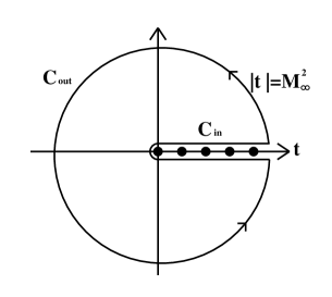
Figure 6: Integration circuit for the moment integrals.

$$\mathcal{A}^{{}^{(n)}}_{{}_{LR}}(Q^{2})\,\,\,\,=\,\,\,\,\lim_{M_{\infty}^{2}\to\infty}\frac{\displaystyle 1}{\displaystyle 2\pi i}\displaystyle{\oint}_{C}\,\,\,\frac{\displaystyle Q^{2n}\,\,dt}{\displaystyle(t+Q^{2})^{n+1}}\,\,\Pi_{{}_{LR}}(t)\,\,\,\,=\,\,\,\,\lim_{M_{\infty}^{2}\to\infty}\displaystyle{\int}_{0}^{M_{\infty}^{2}}\frac{\displaystyle Q^{2n}\,\,dt}{\displaystyle(t+Q^{2})^{n+1}}\,\,\,\frac{\displaystyle 1}{\displaystyle\pi}\mbox{Im}\Pi_{{}_{LR}}(t)\,,$$ (50)

where the integration in $C_{out}$ is assumed to vanish as $M_{\infty}^{2}\to\infty$.

The $V-A$ Green function will be also split into a perturbative and non-perturbative sub-series, where the couplings and masses where formerly fixed in the $V+A$ analysis. In this case, the summation is not positively defined and one needs to specify the parity $\pi_{j}$ of every state. We will consider a spectrum of multiplets with alternating parity where the lowest state is a vector, this is, $\pi_{j}=(-1)^{j}$. At high euclidean momenta $M_{p}^{2}\ll Q^{2}\ll M_{\infty}^{2}$, the perturbative sub-series shows the structure

$$\begin{array}[]{rl}\Delta\Pi_{{}_{LR}}(-Q^{2})_{{}_{pert.}}^{{}^{N_{C}\to\infty}}\,\,\,\,=&\,\,\,\,\displaystyle{\sum_{m=1}^{\infty}}\,\frac{\displaystyle\Delta\langle\,{\cal O}_{{}_{(2m)}}^{{}^{LR}}\,\rangle^{{}^{pert.}}}{\displaystyle Q^{2m}}\,\,,\end{array}$$ (51)

where no dimension-zero term arises since both the vector and axial correlators reproduce the pQCD expression. The non-perturbative part of the series can be analytically expanded without further problems and the summation of both contributions must match the OPE through the constraints

$$\begin{array}[]{rcl}\langle\,{\cal O}_{{}_{(2)}}^{{}^{LR}}\,\rangle\quad=&\quad\Delta\langle\,{\cal O}_{{}_{(2)}}^{{}^{LR}}\,\rangle^{{}^{pert.}}\,\,\,-\,\,\,F^{2}\,\,\,+\,\,\,\displaystyle{\sum_{j=1}^{p}}\,[-\pi_{j}]\,F_{j}^{2}&=\,\,\,0\,,\\ \langle\,{\cal O}_{{}_{(4)}}^{{}^{LR}}\,\rangle\quad=&\qquad\Delta\langle\,{\cal O}_{{}_{(4)}}^{{}^{LR}}\,\rangle^{{}^{pert.}}\,\,\,\,\,\,-\,\,\,\,\,\,\displaystyle{\sum_{j=1}^{p}}\,[-\pi_{j}]\,F_{j}^{2}\,M_{j}^{2}&=\,\,\,0\,.\\ \langle\,{\cal O}_{{}_{(6)}}^{{}^{LR}}\,\rangle\quad=&\qquad\Delta\langle\,{\cal O}_{{}_{(6)}}^{{}^{LR}}\,\rangle^{{}^{pert.}}\,\,\,\,\,\,+\,\,\,\,\,\,\displaystyle{\sum_{j=1}^{p}}\,[-\pi_{j}]\,F_{j}^{2}\,M_{j}^{4}&=\,\,\,-\,4\,\pi\,\alpha_{s}\,\langle\,\bar{q}q\,\rangle^{2}\,\,\,<\,\,\,0\,.\end{array}$$ (52)

4.3 Study of some hadronical models for the spectrum

In this section, we will study some of the current models for the meson spectrum. The resonances with masses in the low energy region ($M_{n}^{2}\mathrel{\hbox to0.0pt{\lower 4.0pt\hbox{\hskip 1.0pt$\sim$}\hss}\raise 1.0pt\hbox{$<$}}2$ GeV²) are susceptible to stronger deviation with respect to the expected asymptotic behaviour $M_{n}^{2}=f(n)$ for high values of $n$. Below $2$ GeV², only two resonance multiplets are found, corresponding to the vector $\rho(770)$ and the axial–vector $a_{1}(1260)$ [65]. The mass spectrum $M_{n}^{2}$ with $n\geq 3$ is interpolated through the first two multiplets above 2 GeV², namely $\rho(1450)$ with $M_{3}^{2}=M_{\rho^{\prime}}^{2}\simeq 1.45^{2}$ and $a_{1}(1640)$ with $M_{4}^{2}=M_{a_{1}^{\prime}}^{2}\simeq 1.64$ GeV² [65]. We will include in the perturbative sub-series the multiplets with $n>p=2$, leaving $M_{1}^{2}=M_{\rho}^{2}$ and $M_{2}^{2}=M_{a_{1}}^{2}$ for the non-perturbative part of the resonance series.

In order to obtain the contribution to the condensates from the perturbative sub-series we will analyse the $V+A$ and $V-A$ Adler functions from $\Delta\Pi^{{}^{N_{C}\to\infty}}_{{}_{pert.}}$ minus the pQCD amplitude, $(\Delta\mathcal{A}(Q^{2})^{{}^{N_{C}\to\infty}}_{{}_{pert.}}-\mathcal{A}(Q^{2})^{{}^{pQCD}})$. We will work only up to ${\cal O}(\alpha_{s})$ in the pQCD distribution so ${\cal O}(\alpha_{s}^{2})$ uncertainties are expected in the derivation of the condensates. Considering the Adler function avoids complications like renormalization scale dependences or absolute convergence of the resonance series. Nevertheless, the $V-A$ measurement is utterly improved by a cross-check analysis of $\Pi_{{}_{LR}}(-Q^{2})$.

We perform the interpolation $(\Delta\mathcal{A}(Q^{2}_{\ell})_{{}_{pert.}}^{{}^{N_{C}\to\infty}}-\mathcal{A}(Q^{2}_{\ell})^{{}^{pQCD}})=\displaystyle{\sum_{m=1}^{8}}\frac{\displaystyle m\,\,\Delta\langle\,{\cal O}_{{}_{(2m)}}\,\rangle^{{}^{pert.}}}{\displaystyle Q^{2m}_{\ell}}$ through eight points $Q^{2}_{\ell}=Q^{2}_{1}+\Delta Q^{2}\,(\ell-1)$, with $Q^{2}_{1}=4$ GeV², $\Delta Q^{2}=0.025$ GeV² and $\ell=1,2...8$ From these eight constraints we extract the perturbative contribution to the first eight condensates $\Delta\langle\,{\cal O}_{{}_{(2m)}}\,\rangle^{{}^{pert.}}$. The interpolating point are varied to ${Q^{2}_{1}=2,\,3,\,5,\,6}$ GeV² in order to check the consistence of the procedure and the size of the uncertainties. It is not possible to go to higher or lower energies since, respectively, on one hand, the ${\cal O}(\alpha_{s}^{2})$ corrections become comparable to the ${\cal O}(1/Q^{6})$ terms and, on the other, the OPE series breaks down within the very low energy range. The central values of the results represent the output for $Q^{2}_{1}=4$ GeV² whereas the error bars express the spreading coming from the analysis at different energies, providing an estimate of the ${\cal O}(\alpha_{s})$ corrections. The errors in the condensates of dimension two, four and six coming from neglecting the $1/Q^{2m}$ terms with dimension beyond $2m=16$ and from the duality violating terms are expected to be rather suppressed. We will make some considerations about the duality violations in the analysis of the five dimensional model although a more exhaustive analysis can be found in Ref. [21].

4.3.1 $QCD_{\infty}$ in $1+1$ dimensions

In the pioneer work on large $N_{C}$ [12], QCD was study at $N_{C}\to\infty$ in a configuration space of dimension $1+1$. In this case the spectrum could be solved and followed an asymptotic behaviour with constant squared mass inter-spacing, $\delta M_{n}^{2}=\delta\Lambda^{2}$. A similar type of spectrum appears as well in different QCD models [30, 34, 37]. We will consider $M_{n}^{2}=\Lambda^{2}+n\,\delta\Lambda^{2}$ for $n\geq 3$, with $\delta\Lambda^{2}=(M_{a_{1}^{\prime}}^{2}-M_{\rho^{\prime}}^{2})$ and $\Lambda^{2}=M_{\rho^{\prime}}^{2}-3\,\delta\Lambda^{2}$.

If one remains at ${\cal O}(\alpha_{s}^{0})$ the imaginary part of the pQCD correlator is just a constant and therefore all the couplings are equal to $F_{n}^{2}=\frac{N_{C}}{12\pi^{2}}\,\cdot\,\delta\Lambda^{2}\simeq(122$ MeV$)^{2}$. Thence, the perturbative sub-series contributions to the condensates derived from the numerical analysis are

$$\Delta\langle\,{\cal O}_{{}_{(2)}}^{{}^{LL}}\,\rangle^{{}^{pert.}}\quad= \quad\left(-45.816^{+0.040}_{-0.011}\right)\cdot 10^{-3}\mbox{ GeV}^{2}\quad \sim\quad\,\,-\,5\,F^{2}\,,$$

$$\Delta\langle\,{\cal O}_{{}_{(4)}}^{{}^{LL}}\,\rangle^{{}^{pert.}}\quad= \quad\left(41.00^{+0.22}_{-0.40}\right)\cdot 10^{-3}\mbox{ GeV}^{4}\quad \sim\quad\,\,\,8\,F^{2}\,M_{\rho}^{2}\,,$$

$$\Delta\langle\,{\cal O}_{{}_{(2)}}^{{}^{LR}}\,\rangle^{{}^{pert.}}\,\,\quad= \quad\left(7.4349^{+0.0011}_{-0.0060}\right)\cdot 10^{-3}\mbox{ GeV}^{2}\quad \sim\quad\,\,F^{2}\,,$$

$$\Delta\langle\,{\cal O}_{{}_{(4)}}^{{}^{LR}}\,\rangle^{{}^{pert.}}\quad= \quad\left(-13.43^{+0.05}_{-0.12}\right)\cdot 10^{-3}\mbox{ GeV}^{4}\quad \sim\quad\,\,-\,3\,F^{2}\,M_{\rho}^{2}\,,$$

$$\Delta\langle\,{\cal O}_{{}_{(6)}}^{{}^{LR}}\,\rangle^{{}^{pert.}}\quad= \quad\left(23.4^{+0.9}_{-1.1}\right)\cdot 10^{-3}\mbox{ GeV}^{6}\quad \sim\quad\,\,8\,F^{2}\,M_{\rho}^{4}\,.$$ (53)

In this model, one may actually compute the exact value of the condensates coming from the perturbative sub-series [21, 33]:

$$\Delta\langle\,{\cal O}_{{}_{(2m)}}^{{}^{LL}}\,\rangle^{{}^{pert.}}\,\, = \,\,\frac{\displaystyle(-1)^{m}}{\displaystyle m}\,\,\frac{\displaystyle N_{C}}{\displaystyle 12\pi^{2}}\left(\delta\Lambda^{2}\right)^{m}\,\,B_{m}\left(\frac{M_{\rho^{\prime}}^{2}}{\delta\Lambda^{2}}\right)\,,$$

$$\Delta\langle\,{\cal O}_{{}_{(2m)}}^{{}^{LR}}\,\rangle^{{}^{pert.}}\,\, = \,\,\frac{\displaystyle(-1)^{m}}{\displaystyle m}\,\,\frac{\displaystyle N_{C}}{\displaystyle 24\pi^{2}}\left(2\,\delta\Lambda^{2}\right)^{m}\,\,\left[\,B_{m}\left(\frac{M_{\rho^{\prime}}^{2}}{2\,\delta\Lambda^{2}}\right)\,-\,B_{m}\left(\frac{M_{a_{1}^{\prime}}^{2}}{2\,\delta\Lambda^{2}}\right)\,\right]\,,$$ (54)

being     $B_{m}(x)$     the    Bernoulli   polynomials     ($B_{1}(x)=x-\frac{1}{2}$,    $B_{2}(x)=x^{2}-x+\frac{1}{6}$,     ${B_{3}(x)=x^{3}-\frac{3}{2}x^{2}+\frac{1}{2}x,\,...}$). For our choice of parameters one finds

$$\Delta\langle\,{\cal O}_{{}_{(2)}}^{{}^{LL}}\,\rangle^{{}^{pert.}}\,\,\,\,= \,\,-\,\frac{\displaystyle N_{C}}{\displaystyle 12\pi^{2}}\,M_{\rho^{\prime}}^{2}\,\left[1-\frac{\delta\Lambda^{2}}{2\,M_{\rho^{\prime}}^{2}}\right]\,\, =\,\,\,\,-45.821\cdot 10^{-3}~{}\mbox{GeV}^{2}\,,$$

$$\Delta\langle\,{\cal O}_{{}_{(4)}}^{{}^{LL}}\,\rangle^{{}^{pert.}}\,\,\,\,= \,\,\,\frac{\displaystyle 1}{\displaystyle 2}\,\frac{\displaystyle N_{C}}{\displaystyle 12\pi^{2}}\,M_{\rho^{\prime}}^{4}\,\left[1-\frac{\delta\Lambda^{2}}{M_{\rho^{\prime}}^{2}}+\frac{(\delta\Lambda^{2})^{2}}{2\,M_{\rho^{\prime}}^{4}}\right]\,\, =\,\,\,\,41.08\cdot 10^{-3}~{}\mbox{GeV}^{4}\,,$$

$$\Delta\langle\,{\cal O}_{{}_{(2)}}^{{}^{LR}}\,\rangle^{{}^{pert.}}\,\,\,\,= \,\,\frac{\displaystyle N_{C}}{\displaystyle 24\pi^{2}}\,\delta\Lambda^{2}\,\, =\,\,\,\,7.4357\cdot 10^{-3}~{}\mbox{GeV}^{2}\,,$$

$$\Delta\langle\,{\cal O}_{{}_{(4)}}^{{}^{LR}}\,\rangle^{{}^{pert.}}\,\,\,\,= \,\,-\,\frac{\displaystyle N_{C}}{\displaystyle 24\pi^{2}}\,\delta\Lambda^{2}\,M_{\rho^{\prime}}^{2}\,\left[1-\frac{\delta\Lambda^{2}}{2\,M_{\rho^{\prime}}^{2}}\right]\,\, =\,\,\,\,-13.45\cdot 10^{-3}~{}\mbox{GeV}^{4}\,,$$

$$\Delta\langle\,{\cal O}_{{}_{(6)}}^{{}^{LR}}\,\rangle^{{}^{pert.}}\,\,\,\,= \,\,\frac{\displaystyle N_{C}}{\displaystyle 24\pi^{2}}\,\delta\Lambda^{2}\,M_{\rho^{\prime}}^{4}\,\left[1-\frac{\delta\Lambda^{2}}{M_{\rho^{\prime}}^{2}}\right]\,\, =\,\,\,\,23.7\cdot 10^{-3}~{}\mbox{GeV}^{6}\,,$$

in total agreement with our former numerical calculation. This provides a check of the accuracy that will make our next numerical calculations reliable. The $V-A$ condensates depend linearly on $\delta M_{j}^{2}=\delta\Lambda^{2}$ and both $\Delta\langle\,{\cal O}_{{}_{(2m)}}^{{}^{LL}}\,\rangle^{{}^{pert.}}$ and $\Delta\langle\,{\cal O}_{{}_{(2m)}}^{{}^{LR}}\,\rangle^{{}^{pert.}}$ have a strong dependence on the mass of the lowest state included in the perturbative sub-series, $M_{\rho^{\prime}}$. In the limit $\frac{\delta M_{j}^{2}}{M_{\rho^{\prime}}^{2}}\to 0$, one recovers exactly the pQCD expression $\Pi(-Q^{2})^{{}^{pQCD}}_{{}_{pert.}}$ at ${\cal O}(\alpha_{s}^{0})$ from Eq. (38), with $\Delta\langle\,{\cal O}_{{}_{(2m)}}^{{}^{LL}}\,\rangle^{{}^{pert.}}=\frac{\displaystyle(-1)^{m}}{\displaystyle m}\,t_{p}^{m}$ and $\Delta\langle\,{\cal O}_{{}_{(2m)}}^{{}^{LR}}\,\rangle^{{}^{pert.}}=0$, being $t_{p}=M_{\rho^{\prime}}^{2}$. The condensates result naturally of the expected size without imposing further constraints, pointing out the close relation between the different QCD scales, hadronic masses, mass inter-spacings, couplings and condensates.

We will take $F=92.4$ MeV, $M_{\rho}=0.77$ GeV, the asymptotic spectrum $M_{n}^{2}=\Lambda^{2}+n\,\delta\Lambda^{2}$ for $n\geq 3$ and the pQCD correlator $\frac{1}{\pi}$Im$\Pi_{{}_{LL}}(q^{2})$ as inputs, and the parameters $F_{\rho},\,F_{a_{1}}$ and $M_{a_{1}}$ will be left as free parameters. They can be recovered by demanding that the condensates $\langle\,{\cal O}_{{}_{(2)}}^{{}^{LL}}\,\rangle$, $\langle\,{\cal O}_{{}_{(2)}}^{{}^{LR}}\,\rangle$ and $\langle\,{\cal O}_{{}_{(4)}}^{{}^{LR}}\,\rangle$ are zero. For a general resonance model, Eqs. (46) and (52) yield the relations

$$\begin{array}[]{rl}F_{\rho}^{2}\,\,=&\,\,-\,\,\frac{\displaystyle 1}{\displaystyle 2}\,\,\left(\Delta\langle\,{\cal O}_{{}_{(2)}}^{{}^{LL}}\,\rangle^{{}^{pert.}}+\Delta\langle\,{\cal O}_{{}_{(2)}}^{{}^{LR}}\,\rangle^{{}^{pert.}}\right)\,,\\ \\ F_{a_{1}}^{2}\,\,=&\,\,\,\,-\,\,\frac{\displaystyle 1}{\displaystyle 2}\,\,\left(\Delta\langle\,{\cal O}_{{}_{(2)}}^{{}^{LL}}\,\rangle^{{}^{pert.}}-\Delta\langle\,{\cal O}_{{}_{(2)}}^{{}^{LR}}\,\rangle^{{}^{pert.}}\right)\,\,\,\,-\,\,\,\,F^{2}\,,\\ \\ M_{a_{1}}^{2}\,\,=&\frac{\displaystyle F_{\rho}^{2}\,M_{\rho}^{2}\,-\,\Delta\langle\,{\cal O}_{{}_{(4)}}^{{}^{LR}}\,\rangle^{{}^{pert.}}}{\displaystyle F_{a_{1}}^{2}}=M_{\rho}^{2}\left\{\frac{\displaystyle\,-\,\frac{\displaystyle 1}{\displaystyle 2}\,\left(\Delta\langle\,{\cal O}_{{}_{(2)}}^{{}^{LL}}\,\rangle^{{}^{pert.}}+\Delta\langle\,{\cal O}_{{}_{(2)}}^{{}^{LR}}\,\rangle^{{}^{pert.}}\right)\,-\,\frac{\displaystyle\Delta\langle\,{\cal O}_{{}_{(4)}}^{{}^{LR}}\,\rangle^{{}^{pert.}}}{\displaystyle M_{\rho}^{2}}}{\displaystyle\,\,-\,\,\left(\Delta\langle\,{\cal O}_{{}_{(2)}}^{{}^{LL}}\,\rangle^{{}^{pert.}}-\Delta\langle\,{\cal O}_{{}_{(2)}}^{{}^{LR}}\,\rangle^{{}^{pert.}}\right)\,\,\,\,-\,\,\,\,F^{2}\,\,}\right\}.\end{array}$$ (56)

In our case at ${\cal O}(\alpha_{s}^{0})$ one finds

$$F_{\rho}=138.5\mbox{ MeV}\,,\qquad F_{a_{1}}=134.5\mbox{ MeV}\,,\qquad M_{a_{1}}\,\,=\,\,1172\mbox{ MeV}\,.$$ (57)

The couplings remain of the order of the asymptotic value $F_{\rho}\sim F_{a_{1}}\sim F_{j\geq 3}$, falling both resonance couplings and axial-vector mass within the expected range of values obtained in former phenomenological analysis [41, 57, 63, 65]. These light states, laying by the non-perturbative QCD regime, suffer slight deviations from the asymptotic behaviour in such a way that the OPE is exactly recovered.

The short distance matching fixes all the parameters in our analysis, providing a prediction for the condensates of higher dimension through Eqs. (46) and (52):

$$\langle\,{\cal O}_{{}_{(4)}}^{{}^{LL}}\,\rangle\,\,\,=\,\,\,4.87\cdot 10^{-3}\mbox{ GeV}^{4}\,,\qquad\langle\,{\cal O}_{{}_{(6)}}^{{}^{LR}}\,\rangle\,\,\,=\,\,\,-\,3.63\cdot 10^{-3}\mbox{ GeV}^{6}\,.$$ (58)

They  already   fall  pretty  near   the   usual  determinations  $\langle\,{\cal O}_{{}_{(4)}}^{{}^{LL}}\,\rangle\simeq 1.2\cdot 10^{-3}$ GeV⁴ [11]  and  ${\langle\,{\cal O}_{{}_{(6)}}^{{}^{LR}}\,\rangle\simeq-3.8\cdot 10^{-3}}$ GeV⁶ [8].

	1+1 $QCD_{\infty}$	5D–spectrum	Conv. WSR1	Conv. WSR2
$\Delta\langle\,{\cal O}_{{}_{(2)}}^{{}^{LL}}\,\rangle^{{}^{pert.}}$ ($10^{-3}$ GeV2)	$-46.9^{+1.7}_{-1.9}$	$-68^{+5}_{-4}$	$-37.4^{+2.1}_{-3.0}$	$-28\pm 6$
$\Delta\langle\,{\cal O}_{{}_{(4)}}^{{}^{LL}}\,\rangle^{{}^{pert.}}$ ($10^{-3}$ GeV4)	$8^{+23}_{-18}$	$140^{+70}_{-60}$	$-30\pm 40$	$-80^{+70}_{-110}$
$\Delta\langle\,{\cal O}_{{}_{(2)}}^{{}^{LR}}\,\rangle^{{}^{pert.}}$ ($10^{-3}$ GeV2)	$8.3771^{+0.0021}_{-0.0070}$	$6.832^{+0.003}_{-0.006}$	$10.902^{+0.005}_{-0.008}$	$14.058^{+0.008}_{-0.011}$
$\Delta\langle\,{\cal O}_{{}_{(4)}}^{{}^{LR}}\,\rangle^{{}^{pert.}}$ ($10^{-3}$ GeV4)	$-15.15^{+0.14}_{-0.08}$	$-12.34^{+0.12}_{-0.11}$	$-19.90^{+0.18}_{-0.21}$	$-29.97^{+0.30}_{-0.25}$
$\Delta\langle\,{\cal O}_{{}_{(6)}}^{{}^{LR}}\,\rangle^{{}^{pert.}}$ ($10^{-3}$ GeV6)	$26.5\pm 1.3$	$21.7^{+2.0}_{-1.1}$	$34.9^{+4.0}_{-1.6}$	$46.2^{+6.0}_{-2.2}$

Table 1: Contributions from the perturbative sub-series to the condensates within different hadronical models. The columns with Converging WSR1 and WSR2 corresponds to squared mass inter-spacings of the form ${\delta M_{n}^{2}\sim 1/\sqrt{n}}$ and ${\delta M_{n}^{2}\sim 1/n}$, respectively. All the amplitudes are considered up to ${\cal O}(\alpha_{s})$.

	1+1 $QCD_{\infty}$	5D–spectrum	Conv. WSR1	Conv. WSR2
$F_{\rho}$ (MeV)	$139\pm 3$	$174^{+5}_{-7}$	$115^{+7}_{-5}$	$83^{+16}_{-20}$
$F_{a_{1}}$ (MeV)	$138\pm 3$	$169^{+6}_{-8}$	$125^{+6}_{-4}$	$111^{+12}_{-14}$
$M_{a_{1}}$ (MeV)	$1180^{+17}_{-19}$	$1029^{+19}_{-13}$	$1330\pm 40$	$1560^{+180}_{-120}$
$\langle\,{\cal O}_{{}_{(4)}}^{{}^{LL}}\,\rangle$ ($10^{-3}$ GeV4)	$-30^{+22}_{-30}$	$100^{+70}_{-60}$	$-70\pm 40$	$-120^{+70}_{-110}$
$\langle\,{\cal O}_{{}_{(6)}}^{{}^{LR}}\,\rangle$ ($10^{-3}$ GeV6)	$-3.7^{+0.8}_{-0.3}$	$0.3^{+2.2}_{-1.5}$	$-9.7^{+1.5}_{-0.7}$	$-24^{+7}_{-8}$

Table 2: Predictions for the two first resonance multiplets –$\rho(770)$ and $a_{1}(1260)$– within each model for the inputs $F=92.4$ MeV and $M_{\rho}=0.77$ GeV. We consider the amplitudes up to ${\cal O}(\alpha_{s})$.

The calculation can be taken up to ${\cal O}(\alpha_{s})$ so the $\alpha_{s}(Q^{2})$ running in $\mathcal{A}^{{}^{(n)}}_{{}_{LL}}(Q^{2})$ is recovered. The next-to-leading order computation is relevant in order to improve the determinations of the condensates $\langle\,{\cal O}_{{}_{(4)}}^{{}^{LL}}\,\rangle$ and $\langle\,{\cal O}_{{}_{(6)}}^{{}^{LR}}\,\rangle$, checking the impact coming from the perturbative QCD corrections in $\alpha_{s}$. The contributions to the condensates at this order that come from the perturbative sub-series may be found in the first column of Table (1), where we have considered the same values for $\alpha_{s}(Q^{2})$ and the pQCD correlator as in Section 3. In Table (2), it is possible to find the corresponding $\rho(770)$ and $a_{1}(1260)$ couplings and masses, and the value of the condensates $\langle\,{\cal O}_{{}_{(4)}}^{{}^{LL}}\,\rangle$ and $\langle\,{\cal O}_{{}_{(6)}}^{{}^{LR}}\,\rangle$ derived from the short distance matching $\langle\,{\cal O}_{{}_{(2)}}^{{}^{LL}}\,\rangle=\langle\,{\cal O}_{{}_{(2)}}^{{}^{LR}}\,\rangle=\langle\,{\cal O}_{{}_{(4)}}^{{}^{LR}}\,\rangle=0$. Small variations arise with respect to the ${\cal O}(\alpha_{s}^{0})$ result, as expected if the asymptotic behaviour of resonance parameters depends smoothly on $\alpha_{s}$. However, the ${\cal O}(\alpha_{s}^{2})$ uncertainties increase the error in the $V+A$ condensates by two orders of magnitude, where $\langle\,{\cal O}_{{}_{(4)}}^{{}^{LL}}\,\rangle$ becomes now negative, pointing out the necessity of working at that order if more accurate determinations are required.

4.3.2 Five–dimensional spectrum

Another available scenario that has appeared recently is the one provided by models in five dimensions [31, 32]. Here the resonances appear as Kaluza-Klein modes from the quantization of the momentum in the fifth dimension, producing a four dimensional effective spectrum with the dependence $M_{n}^{2}\sim n^{2}$, this is, $\delta M_{n}^{2}\sim n\sim\sqrt{M_{n}^{2}}$. We will use the interpolation $M_{n}=\Lambda+n\,\delta\Lambda$, with $\delta\Lambda=(M_{a_{1}^{\prime}}-M_{\rho^{\prime}})$ and $\Lambda=M_{\rho^{\prime}}-3\delta\Lambda$. The corresponding contributions to condensates coming from the perturbative sub-series are shown in Table (1). Taking these values and the inputs $F$ and $M_{\rho}$ one derives the resonance parameters and the predictions for the condensates shown in Table (2). One finds an acceptable value for the $a_{1}(1260)$ mass although the values of the resonance couplings go high above the usual determinations. The predictions for the condensates $\langle\,{\cal O}^{{}^{LL}}_{{}_{(4)}}\,\rangle$ and $\langle\,{\cal O}^{{}^{LR}}_{{}_{(6)}}\,\rangle$ appear slightly shifted with respect to 1+1 $QCD_{\infty}$ though the positive sign for $\langle\,{\cal O}^{{}^{LL}}_{{}_{(4)}}\,\rangle$ is properly restored.

It is important to remark that this is not exactly a five dimensional calculation but an effective study of its spectrum. The series of infinite resonances in the 5D–theory are not regulated in the way of our cut-off, yielding some extra features as the existence of infinite Weinberg sum rules [32]. In the strict five dimensional calculation one must handle the full Kaluza-Klein pile (including also the first two resonances) with its precise dependence. For instance, one has $M_{n}^{2}=\frac{\pi^{2}}{4\,l_{1}^{2}}\left(n+\frac{1}{2}\right)^{2}$ and $F_{n}^{2}=\frac{N_{C}}{24\pi^{2}}\cdot\frac{\pi^{2}}{2\,l_{1}^{2}}\left(n+\frac{1}{2}\right)$ for the RS1 metric in Ref. [32], being $l_{1}=3\pi/(4\,M_{\rho})$ the position of the infrared brane. This exact structure of the spectrum generates a $V-A$ amplitudes without condensates,

$$\Pi_{{}_{LR}}(-Q^{2})\,\,\,\,\stackrel{{\scriptstyle Q^{2}\gg M_{\rho}^{2}}}{{\simeq}}\,\,\,\,-\,\frac{\displaystyle N_{C}}{\displaystyle 12\pi}\,\,\exp{\left[\,-\,\frac{\displaystyle 3\pi\,Q}{\displaystyle 2\,M_{\rho}}\,\right]}\,.$$ (59)

For the perturbative QCD range of euclidean momenta the exponential factor produce a huge suppression (${\cal O}(10^{-4})$ already for $Q^{2}=2$ GeV² and ${\cal O}(10^{-9})$ for $Q^{2}=10$ GeV²). Variations on the lightest Kaluza-Klein modes due to ${\cal O}(\alpha_{s})$ corrections (present analysis) or perturbations on the metric [32] result into the appearance of $1/Q^{2m}$ power terms. The duality violating term in Eq. (59) affects our numerical OPE interpolation beyond the dimension–sixteen condensate, so the determinations are still safe. Nevertheless, the exponential may become enhanced with respect to the $1/Q^{2m}$ terms when considering moment integrals $\mathcal{A}^{{}^{(k)}}(Q^{2})$ or components $\mathcal{B}^{{}^{(k)}}(Q^{2})$ for large values of $k$. Eventual contributions might produce observable modifications to the usual OPE calculations [21].

4.3.3 Converging Weinberg sum rules

For   a general  spectrum  and  within  our considered   cut-off regularization,  large $N_{C}$ QCD  do not obey   in general the two Weinberg sum rules (WSR),  $\displaystyle{\int}_{0}^{\infty}dt\,\frac{1}{\pi}$Im$\Pi_{{}_{LR}}(t)=0$   and  ${\displaystyle{\int}_{0}^{\infty}dt\,\,t\,\frac{1}{\pi}\mbox{Im}\Pi_{{}_{LR}}(t)=0}$, since the infinite summations of resonances are not convergent. The fulfilling of these two WSR immediately implies a dominant behaviour $\Pi_{{}_{LR}}(-Q^{2})\sim\frac{\displaystyle 1}{\displaystyle Q^{6}}$ in the deep euclidean.

One may consider the covergence of the two WSR as an available hypothesis for the model building. In this case, the summations

$${\int}_{0}^{\infty}\,dt\,\,\,t^{m}\,\,\,\frac{\displaystyle 1}{\displaystyle\pi}\mbox{Im}\Pi_{{}_{LR}}(t)\,\,\,\,=\,\,\,\,\,\,\,\,-\,\,F^{2}\,\delta^{m,0}\,\,+\,\,\displaystyle{\sum_{j=1}^{\infty}}\,[-\pi_{j}]\,\,F_{j}^{2}\,\,(M_{j}^{2})^{m}\,,$$ (60)

must be zero (and therefore converging) for $m=0$ and  $m=1$ [16]. This demands  that $F_{n}^{2}\stackrel{{\scriptstyle n\to\infty}}{{\longrightarrow}}0$ and  $F_{n}^{2}\,M_{n}^{2}\stackrel{{\scriptstyle n\to\infty}}{{\longrightarrow}}0$.  If we desire just two Weinberg sum rules,  then $F_{n}^{2}\,(M_{n}^{2})^{m}$ must not vanish when $n\to\infty$ for $m\geq 2$.  If the asymptotic value of the couplings is fixed through  ${F_{n}^{2}\simeq\delta M_{n}^{2}\,\cdot\,\frac{1}{\pi}\mbox{Im}\Pi_{{}_{LL}}(M_{n}^{2})^{{}^{pQCD}}\sim\delta M_{n}^{2}}$, one finds in Eq. (60) that $F_{n}^{2}\,(M_{n}^{2})^{m}\sim\delta M_{n}^{2}\cdot(M_{n}^{2})^{m}$ must vanish when $M_{n}^{2}\to\infty$ just for $m=0$ and $m=1$; the inter-spacing $\delta M_{n}^{2}$ must tend to zero as $n$ goes to infinity faster than $\delta M_{n}^{2}\sim\frac{1}{\sqrt{n}}\sim\frac{1}{M_{n}^{2}}$ and slower than $\delta M_{n}^{2}\sim\frac{1}{n}\sim e^{-M_{n}^{2}}$.

We will analyse both extreme cases through two different modelings of the spectrum.   On one hand,   we   will   consider   the model WSR1,  owning   the   spectrum  ${M_{n}^{2}=\Lambda^{2}+\sqrt{n}\,\delta\Lambda^{2}}$ with  ${\delta\Lambda^{2}=(M_{a_{1}^{\prime}}^{2}-M_{\rho^{\prime}}^{2})/(\sqrt{4}-\sqrt{3})}$ and  $\Lambda^{2}=M_{\rho^{\prime}}^{2}-\sqrt{3}\,\,\delta\Lambda^{2}$.  This  provides  the limit   case  ${\delta M_{n}^{2}\sim\frac{1}{\sqrt{n}}\sim\frac{1}{M_{n}^{2}}}$.  For the other limit   case we consider the model WSR2,   with  spectrum  ${M_{n}^{2}=\Lambda^{2}+\delta\Lambda^{2}\ln{(n)}}$, with $\delta\Lambda^{2}=(M_{a_{1}^{\prime}}^{2}-M_{\rho^{\prime}}^{2})/(\ln{(4)}-\ln{(3)})$ and $\Lambda^{2}=M_{\rho^{\prime}}^{2}-\ln{(3)}\,\,\delta\Lambda^{2}$. This model owns the high mass behaviour $\delta M_{n}^{2}\sim\frac{1}{n}\sim e^{-M_{n}^{2}}$.

The results for both kinds of spectrums up to ${\cal O}(\alpha_{s})$ can be found in the third and fourth columns of Tables (1) and (2). The axial-vector mass goes beyond the usual range $1$ GeV$\mathrel{\hbox to0.0pt{\lower 4.0pt\hbox{\hskip 1.0pt$\sim$}\hss}\raise 1.0pt\hbox{$<$}}M_{a_{1}}\mathrel{\hbox to0.0pt{\lower 4.0pt\hbox{\hskip 1.0pt$\sim$}\hss}\raise 1.0pt\hbox{$<$}}1.26$ GeV, whereas the resonance couplings decrease up to unphysical values, what seems to rule out this kind of converging–WSR models.

4.4 Truncated resonance theory and Minimal Hadronical Approximation

The contribution  to  the  OPE  condensates  coming  from  the   high  mass  multiplets  vary   depending  on  the  model   for  the hadronic spectrum.  However,   all  of them   reproduce pQCD   and  generate  contributions  to  the   condensates  of   the   right   size  –the  standard   hadronical   parameters  $F^{2}$ and $M_{\rho}^{2}$–  without  demanding  any  further  fine  tuning,  ${\left|\Delta\langle\,{\cal O}_{{}_{(2m)}}^{{}^{LL}}\,\rangle^{{}^{pert}}\right|\,,\,\,\,\left|\Delta\langle\,{\cal O}_{{}_{(2m)}}^{{}^{LR}}\,\rangle^{{}^{pert}}\right|\,\quad\sim\quad{\cal O}\left(F^{2}(M_{\rho}^{2})^{m-1}\right)}$.

The matching with the OPE can be improved through a more exhaustive scanning of the resonance parameters (e.g. $\Lambda^{2}$ and $\delta\Lambda^{2}$ in the 1+1 $QCD_{\infty}$ spectrum) and analysing possible corrections to the asymptotic dependence of $M_{n}^{2}$. Likewise, the second vector multiplet, with $M_{\rho^{\prime}}^{2}\sim 2$ GeV², lies by the border of the non-perturbative QCD region and it may suffer still sizable variations with respect to the asymptotic behaviour. A deeper study should consider the three resonances $\rho(770)$, $a_{1}(1260)$ and $\rho(1450)$ apart, within the non-perturbative sub-series.

Nonetheless, in many situations the inclusion of the full infinite pile of hadronic states is quite involved. The information about higher mass states is rather poor, so one cannot yield a precise determination of the perturbative sub-series $\Delta\Pi(-Q^{2})_{{}_{pert.}}^{{}^{N_{C}\to\infty}}=\Pi(-Q^{2})^{{}^{pQCD}}+\displaystyle{\sum_{m=1}^{\infty}}\frac{\displaystyle\Delta\langle\,{\cal O}_{{}_{(2m)}}\,\rangle^{{}^{pert.}}}{\displaystyle Q^{2m}}$. This forces to truncate the resonance tower and to consider just a finite number of states, those in $\Delta\Pi(-Q^{2})_{{}_{non-p.}}^{{}^{N_{C}\to\infty}}$, setting $\Delta\Pi(-Q^{2})_{{}_{pert.}}^{{}^{N_{C}\to\infty}}=0$. The separation between perturbative and non-perturbative series is not clear and, formally, one may consider as many states as desired within $\Delta\Pi(-Q^{2})_{{}_{non-p.}}^{{}^{N_{C}\to\infty}}$. Moreover, in order to reproduce the right long/short–distance behaviour of QCD ($\chi PT$/OPE) one needs to include at least a minimal number of multiplets in the resonance theory. This is denoted as Minimal Hadronical Approximation (MHA) [40]. Strictly speaking, MHA refers only to Green-functions which are order parameters although some ansate replace $\Delta\Pi(-Q^{2})_{{}_{pert.}}^{{}^{N_{C}\to\infty}}$ by a pQCD continuum [38, 39].

In the MHA analysis of the $V-A$ correlator, one needs to keep at least the Goldstones from the chiral symmetry breaking, together with the first vector and axial-vector multiplets:

$$\Pi_{{}_{LR}}(-Q^{2})^{{}^{N_{C}\to\infty}}\,\,=\,\,-\,\frac{\displaystyle F^{2}}{\displaystyle Q^{2}}\,\,+\,\,\frac{\displaystyle F_{\rho}^{2}}{\displaystyle M_{\rho}^{2}+Q^{2}}\,\,-\,\,\frac{\displaystyle F_{a_{1}}^{2}}{\displaystyle M_{a_{1}}^{2}+Q^{2}}\,\,\,\,+\,\,\,\,{\cal O}\left(\frac{\displaystyle\delta M^{2}}{\displaystyle Q^{2}}\right)\,\,.$$ (61)

The terms ${\cal O}\left(\frac{\delta M^{2}}{Q^{2}}\right)$ from $\Delta\Pi_{{}_{LR}}(-Q^{2})_{{}_{pert.}}^{{}^{N_{C}\to\infty}}$ are dropped out in MHA. Through a short–distance matching to the dominant power behaviour of the OPE ($\Pi_{{}_{LR}}(-Q^{2})\sim 1/Q^{6}$), the values of the lightest resonance parameters are constrained, getting the familiar relations [16, 42, 43],

$$\widetilde{F}_{\rho}^{2}\,-\,\widetilde{F}_{a_{1}}^{2}\,=\,F^{2}\,,\qquad\qquad\widetilde{F}_{\rho}^{2}\,\widetilde{M}_{\rho}^{2}\,-\,\widetilde{F}_{a_{1}}^{2}\,\widetilde{M}_{a_{1}}^{2}\,=0\,.$$ (62)

The couplings and masses are now substituted by some effective parameters ($F_{\rho/a_{1}}\to\widetilde{F}_{\rho/a_{1}}$ and $M_{\rho/a_{1}}\to\widetilde{M}_{\rho/a_{1}}$) where the information of the perturbative sub-series is also encoded. They suffer corrections proportional to $\Delta\langle\,{\cal O}_{{}_{(2m)}}^{{}^{LR}}\,\rangle^{{}^{pert.}}$ with respect to their original values in the full theory and some information is lost since the number of hadronic parameters decreases considerably. For the experimental values $\widetilde{M}_{\rho}=0.77$ GeV and $\widetilde{F}_{\rho}\simeq 154$ MeV, coming from the decay $\rho^{0}\to e^{+}e^{-}$ [41], one finds the predictions $\widetilde{F}_{a_{1}}=\sqrt{\widetilde{F}_{\rho}^{2}-F^{2}}\simeq 123$ MeV, $\widetilde{M}_{a_{1}}=\widetilde{F}_{\rho}\widetilde{M}_{\rho}/\widetilde{F}_{a_{1}}\simeq 964$ MeV and ${\langle\,\widetilde{{\cal O}}_{{}_{(6)}}^{{}^{LR}}\,\rangle=-\frac{\displaystyle\widetilde{F}_{\rho}^{2}}{\displaystyle\widetilde{F}_{a_{1}}^{2}}\,F^{2}\,\widetilde{M}_{\rho}^{4}\simeq-4.7\cdot 10^{-3}}$ GeV⁶.
     A further analysis of the vector and axial form factors [42] leads to ${\widetilde{F}_{\rho}=\sqrt{2}\,F\simeq 131}$ MeV, ${\widetilde{F}_{a_{1}}=F\simeq 92.4}$ MeV, $\widetilde{M}_{a_{1}}=\sqrt{2}\,\widetilde{M}_{\rho}\simeq 1089\mbox{ MeV}$ and $\langle\,\widetilde{{\cal O}}_{{}_{(6)}}^{{}^{LR}}\,\rangle=-2F^{2}\widetilde{M}_{\rho}^{4}\simeq-6\cdot 10^{-3}$ GeV⁶. One must be aware of the intrinsic uncertainty laying in the truncated resonance theory (which must not be misleadingly taken as model dependence). Performing a short–distance matching for a wider set of matrix elements modifies the value of the parameters and one risks to reach inconsistencies between the different constraints, eventually requiring the introduction the next resonance multiplet in the MHA description.

The   difference between  the QCD parameters  in MHA  and those derived   through other techniques  is   just  due  to  the absence of the perturbative part of the resonance series.  The   uncertainty   in   the  MHA  short-distance   matching  to  OPE  is  given   by   the   size  of   ${\Delta\langle\,{\cal O}_{{}_{(2m)}}^{{}^{LR}}\,\rangle^{{}^{pert.}}\sim{\cal O}\left(\delta M^{2}(M_{\rho^{\prime}}^{2})^{m-1}\right)}$. The smooth variation of the resonance parameters from MHA to MHA+$\rho^{\prime}$ [9] hints its close relation with the full large $N_{C}$ resonance theory.

The employment of this approximation has led to a very successful large $N_{C}$ phenomenology [43]: study of vector, axial-vector and scalar form-factors [42, 60], determination of $\chi PT$ couplings [41, 42, 43, 45, 46, 47], description of two–point Green functions [9, 16, 39, 42, 46] and three-point QCD Green functions [44, 45, 48]. In addition, once the theory is well founded at leading order in $1/N_{C}$, unitarity imposes serious constraints on the next-to-leading order effects. Thus, the final state interaction admits a well defined description within the MHA framework [55, 57, 58, 59, 60, 61, 62, 63, 64]. Likewise, some calculations have affronted the problem of the renormalization and the radiative corrections to the couplings at next-to-leading order in $1/N_{C}$ [49, 50, 51, 52, 53, 54, 55].

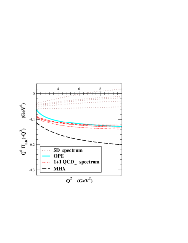
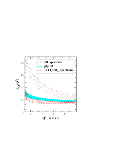
Figure 7: $V-A$ and $V+A$ Adler functions in R$\chi T^{(\infty)}$ up to ${\cal O}(\alpha_{s})$ and within MHA. They are compared to the results from the OPE and pQCD at that order.

5 Space-like region and local duality: resonance theory vs. OPE

In this section we show how the resonance description matches the OPE in the euclidean domain. The 1+1 $QCD_{\infty}$ model and the 5D-spectrum are considered although the first one yields the closest results to phenomenology. One can see on right-hand-side of Fig. (7) the comparison between the ${V+A}$ Adler functions coming from the OPE and the large $N_{C}$ resonance theory. We have plotted $Q^{6}\,\Pi_{{}_{LR}}(-Q^{2})$ on the left-hand-side of Fig. (7) in order to show the short distance $1/Q^{6}$ behaviour in a more transparent way. For the OPE and pQCD, we have taken the values from Section 3, with $V-A$ operators up to dimension twelve. The MHA expression for $\Pi_{{}_{LR}}(-Q^{2})$ is plotted for the values $\widetilde{F}_{\rho}/\sqrt{2}=\widetilde{F}_{a_{1}}=F$ and $\widetilde{M}_{a_{1}}=\sqrt{2}\,\widetilde{M}_{\rho}$.

Although the ${\cal O}(\alpha_{s}^{2})$ uncertainties are still sizable and subleading $1/N_{C}$ effects need to be analysed, the euclidean amplitudes are already sensitive to the different structures of the spectrum. The 1+1 $QCD_{\infty}$ spectrum recovers quite accurately the OPE and pQCD. The amplitude coming from the five dimensional model does not agree for the choice of parameters in this work, pointing out the necessity of a further tuning of $M_{\rho^{\prime}}$ and $M_{a_{1}^{\prime}}$ in order to match the OPE at short distances. Finally, one can see that, although MHA produces a $V-A$ correlator of the right order of magnitude and $1/Q^{6}$ dependence, it does not completely agree the OPE determination. A better agreement is found if the short distance constraints of the form-factors are relaxed and only the two WSR are kept [9]. The inclusion in the MHA of the next resonance multiplet, corresponding to the $\rho(1450)$, improves the $\rho+a_{1}$ calculation and increases the accuracy of the determination [9].

Another way to study the properties of the amplitude in the euclidean region is through its moments at a fixed energy. In Section 3, we showed how the components $\mathcal{B}^{{}^{(k)}}(Q^{2})$ suppress the dependence of the dispersive integral on the spectral function $\frac{1}{\pi}$Im$\Pi(t)$ around $t\sim Q^{2}$. The $\mathcal{B}^{{}^{(k)}}(Q^{2})$ of the physical amplitudes oscillate as $k$ grows and eventually damp off. The OPE is able to follow the physical $\mathcal{B}^{{}^{(k)}}(Q^{2})$ for the first values of $k$ but, for a fixed $Q^{2}$, it breaks down above some $k_{{}_{OPE-lim.}}$. Increasing the energy or considering higher dimension operators allows increasing the range of validity of the OPE, $k_{{}_{OPE-lim}}$.

The large $N_{C}$ resonance framework reaches a much further range, reproducing at the same time the good OPE results for $k\mathrel{\hbox to0.0pt{\lower 4.0pt\hbox{\hskip 1.0pt$\sim$}\hss}\raise 1.0pt\hbox{$<$}}k_{{}_{OPE-lim.}}$. In Figs. (8) and (9), we can see the corresponding components from the experimental ansatz in the $V+A$ and $V-A$ channels compared with the resonance description from the 1+1 $QCD_{\infty}$ spectrum and the 5D spectrum, being again the first one clearly favoured. The situation is manifest in the $V+A$ correlator, where the oscillation in the 5D-model is much wider and one even finds opposite signs for the components of the two resonances models. In the $V-A$ case, it is also compared with the MHA expression, with ${\widetilde{F}_{\rho}/\sqrt{2}=\widetilde{F}_{a_{1}}=F}$ and $\widetilde{M}_{a_{1}}=\sqrt{2}\,\widetilde{M}_{\rho}$. In general, the $\mathcal{B}^{{}^{(k)}}(Q^{2})$ in the large $N_{C}$ resonance theory follow a natural oscillating behaviour. It does not vanish for high values of $k$ since the states own zero width, whereas the physical components eventually damp off due to the non-zero widths of the hadronic states. Nonetheless, through a careful estimate of the first components and their uncertainties, one is already able to distinguish between the different models for the spectrum and their couplings.

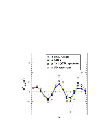
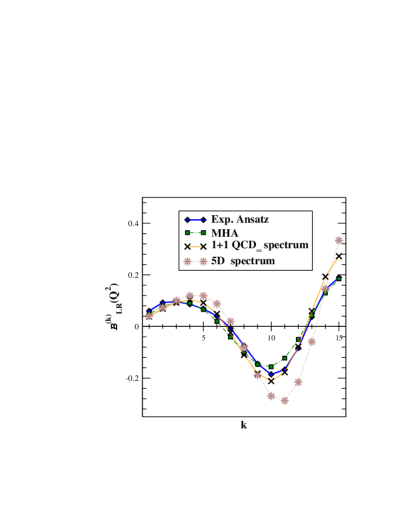
Figure 8: Components $\mathcal{B}^{{}^{(k)}}_{{}_{LR}}(Q^{2})$ of the $V-A$ correlator for $Q^{2}=2$ GeV² and $Q^{2}=10$ GeV². The experimental ansatz is compared to the large $N_{C}$ resonance theory determinations and MHA.

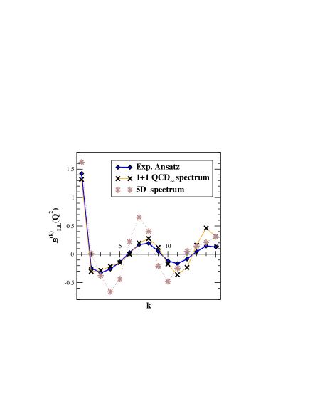
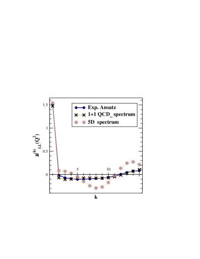
Figure 9: Components $\mathcal{B}^{{}^{(k)}}_{{}_{LL}}(Q^{2})$ of the $V+A$ correlator for $Q^{2}=2$ GeV² and $Q^{2}=10$ GeV². The experimental ansatz is compared to the resonance expression at large $N_{C}$.

6 Time-like region and averaged spectral functions

The QCD interaction at $N_{C}\to\infty$ is so strong that distorts the smooth pQCD spectral functions into a series of narrow-width resonances. However, the higher order corrections in $1/N_{C}$ provide the hadronic states with non-zero widths, so the physical amplitudes become again smooth. However, it is interesting to extract information from the experiment already at leading order in $1/N_{C}$, so we will consider the averaged spectral functions introduced before in Section 2.3. Instead of working with the spectral function $\frac{1}{\pi}$Im$\Pi(t)$ at a given positive energy $t$, it is rather convenient to employ the function $\sigma_{z}(x)$, with the mapping $x=\left(\frac{t-z}{t+z}\right)$. $\sigma_{z}(x)$ is then averaged by the distribution $\xi_{a}(x)$, with dispersion $(\Delta x)^{2}_{\xi_{a}}=\frac{1}{a+3}$. The average $\frac{1}{\pi}$Im$\overline{\Pi}(z)^{{}^{\xi_{a}}}=\langle\,\sigma_{z}\,\rangle_{{}_{\xi_{a}}}$ is essentially provided by the spectral function $\sigma_{z}(x)$ in the interval $|x|\mathrel{\hbox to0.0pt{\lower 4.0pt\hbox{\hskip 1.0pt$\sim$}\hss}\raise 1.0pt\hbox{$<$}}(\Delta x)_{\xi_{a}}$, i.e., by $\frac{1}{\pi}$Im$\Pi(t)$ in the interval $|t-z|\mathrel{\hbox to0.0pt{\lower 4.0pt\hbox{\hskip 1.0pt$\sim$}\hss}\raise 1.0pt\hbox{$<$}}2\,z\,(\Delta x)_{\xi_{a}}$. The interesting peculiarity here is that the averaged correlator only depends on the first $a+1$ moments. As we saw in the former section, the first components $\mathcal{B}^{{}^{k}}(z)$ are mainly governed by the large $N_{C}$ resonance contributions, being the higher orders in $k$ ruled by the subleading effects in $1/N_{C}$.

One may compare the experimental and theoretical $\langle\,\sigma_{z}\,\rangle_{{}_{\xi_{a}}}$ pondered by distributions $\xi_{a}(x)$ with $a$ small enough. This procedure, suppresses the influence of the data away of the center of the distribution, $t=z$. However, if $z$ lays near a resonance peak and $a$ is taken too large, then the distribution $\xi_{a}(x)$ may result too narrow and one has to consider the physical non-zero width of the hadronic state.

This procedure could be useful for the analysis of the spectral functions from $\tau$–decays, where the data reaches just $t\mathrel{\hbox to0.0pt{\lower 4.0pt\hbox{\hskip 1.0pt$\sim$}\hss}\raise 1.0pt\hbox{$<$}}3$ GeV². At low enough energies (for $z\mathrel{\hbox to0.0pt{\lower 4.0pt\hbox{\hskip 1.0pt$\sim$}\hss}\raise 1.0pt\hbox{$<$}}1.5$ GeV² and taking $\xi_{a}(x)$ with $a\sim 8$), the region where there are no experimental data remains on the tail of the distribution $\xi_{a}(x)$, yielding suppressed corrections. The range of energies around the $\rho$ resonance is specially interesting, where very accurate data [22, 23, 24, 25, 26] and an exhaustive theoretical work on the resonance parameters already exists [41, 42, 49, 56, 57, 58, 59, 62].

On Fig. (10), we can see how R$\chi T^{{}^{(\infty)}}$ with the 1+1 $QCD_{\infty}$ spectrum matches pQCD for $z\mathrel{\hbox to0.0pt{\lower 4.0pt\hbox{\hskip 1.0pt$\sim$}\hss}\raise 1.0pt\hbox{$>$}}5$ GeV², where the slight discrepancy below demands a deeper analysis of the contributions from the non-zero dimension operators in the OPE. Actually, the fine agreement with the experimental ansatz around the $\rho(770)$ peak ($z\mathrel{\hbox to0.0pt{\lower 4.0pt\hbox{\hskip 1.0pt$\sim$}\hss}\raise 1.0pt\hbox{$<$}}1$ GeV²) points out again that the values in Table. (2) for the $\rho$ and $a_{1}$ parameters lie on the proper range. For the set of parameters considered in this work, The 5D spectrum shows again a slower convergence and large discrepancies with the experimental ansatz at $z\mathrel{\hbox to0.0pt{\lower 4.0pt\hbox{\hskip 1.0pt$\sim$}\hss}\raise 1.0pt\hbox{$<$}}1$ GeV². MHA is also shown in the $V-A$ case with the couplings $\widetilde{F}_{\rho}/\sqrt{2}=\widetilde{F}_{a_{1}}=F$ and masses $\widetilde{M}_{a_{1}}=\sqrt{2}\,\widetilde{M}_{\rho}$. At $z\mathrel{\hbox to0.0pt{\lower 4.0pt\hbox{\hskip 1.0pt$\sim$}\hss}\raise 1.0pt\hbox{$<$}}1$ GeV², it provides an acceptable approximation of the experimental ansatz averaged amplitude.

For energies beyond $1.5$ GeV² the tail of the distribution $\xi_{a}(x)$ reaches also the resonances with squared masses around $2-3$ GeV² and both MHA and the experimental ansatz with just $\tau$ data loose reliability. This calls out for the inclusion of higher energy $e^{+}e^{-}$ data. A more exhaustive error analysis is also needed in order to yield a precise and accurate determinations of the $\rho(770)$ and $a_{1}(1260)$ parameters at leading order in $1/N_{C}$.

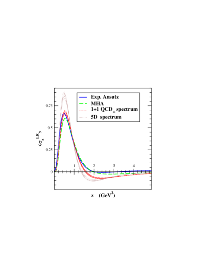
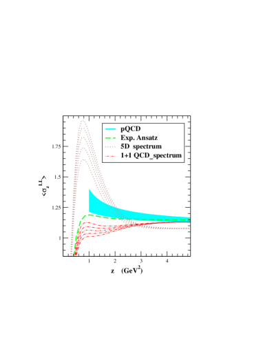
Figure 10: Averaged spectral functions $\frac{1}{\pi}$Im$\overline{\Pi}(z)^{{}^{\xi_{a}}}=\langle\,\sigma_{z}\,\rangle_{{}_{\xi_{a}}}$ for $a=8$.

7 Conclusions

This paper explores the large $N_{C}$ description of QCD through a theory with an infinite number of hadronic states. We show how it is possible to recover the OPE up to order $\alpha_{s}$ in a systematic way, obtaining the corresponding $\alpha_{s}(Q^{2})$ running in $\Pi_{{}_{LL}}(-Q^{2})$. Producing the precise anomalous dimensions in the condensates is still a hard task and the study at ${\cal O}(\alpha_{s}^{2})$ is relegated to next works.

The present analysis is based on three foundations. First, it is assumed that, in the deep euclidean domain, the QCD amplitudes and the different moments can be fairly described through the OPE. Second, the amplitudes in the large $N_{C}$ limit accept a description in terms of an infinite exchange of narrow resonances that embodies the OPE; the correlators are meromorphic functions determined by the positions and residues of an infinite set of real poles. Third, in order to handle the infinite tower of hadronic states one has to assume a given asymptotic structure $M_{n}^{2}=f(n)$ for the spectrum at high energies and a smooth behaviour on $n$ for the resonance couplings. Although we still lack a definitive theoretical explanation of the meson masses, we can nevertheless test (and eventually discard) some of the models currently considered. 1+1 $QCD_{\infty}$ ($M_{n}^{2}\sim n$) and the 5D theories ($M_{n}^{2}\sim n^{2}$) seem to own the most favoured spectrums by the phenomenology, being the first one in closer agreement.

The structure of the mass spectrum imposes constraints on the resonance couplings if we want to recover the pQCD expression for the $V+A$ correlator:

$$F_{n}^{2}\,\,\,\,=\,\,\,\,\delta M_{n}^{2}\,\,\cdot\,\,\left\{\frac{\displaystyle 1}{\displaystyle\pi}\mbox{Im}\Pi_{{}_{LL}}(M_{n}^{2})^{{}^{pQCD}}\,\,\,+\,\,\,{\cal O}\left(\frac{\displaystyle 1}{\displaystyle M_{n}^{2}}\right)\right\}\,.$$

The lightest mass states cannot be fixed through this procedure since pQCD breaks down and the asymptotic dependence of $M_{n}^{2}$ may suffer large $\alpha_{s}$ corrections. The perturbative sub-series containing the high mass resonances is fixed by pQCD and our knowledge on $M_{n}^{2}$. As the pQCD $V+A$ correlator is recovered, the $V-A$ amplitude shows an OPE structure of the form $\Pi_{{}_{LR}}(-Q^{2})\sim\frac{\displaystyle 1}{\displaystyle Q^{2m}}$. A final matching is performed by fixing the values of the lightest resonance parameters in order to ensure that $\Pi_{{}_{LR}}(-Q^{2})$ goes like $1/Q^{6}$ and that the first condensate in $\Pi_{{}_{LL}}(-Q^{2})$ has dimension four. Although the deviations of $F_{\rho}$ and $F_{a_{1}}$ with respect to the asymptotic values of $F_{n}$ are not large, they are essential to match $R\chi T^{(\infty)}$ and the OPE at order $\alpha_{s}$. The 1+1 $QCD_{\infty}$ mass spectrum $M_{n\geq 3}^{2}=\Lambda^{2}+n\,\delta\Lambda^{2}$ yields the couplings

$$F_{\rho}\,=\,139\pm 3\mbox{ MeV }\,,\qquad F_{a_{1}}\,=\,138\pm 3\mbox{ MeV }\,,\qquad M_{a_{1}}\,=\,1180^{+17}_{-19}\mbox{ MeV }\,.$$

The prediction for $\langle\,{\cal O}_{{}_{(6)}}^{{}^{LR}}\,\rangle$ agrees standard OPE determinations but there are still large uncertainties in the $V+A$ sector where a deeper ${\cal O}(\alpha_{s}^{2})$ study needs to be done. Considering pQCD just at ${\cal O}(\alpha_{s}^{0})$ produces small modifications on the resonance parameters, what ensures the stability of the whole procedure under $\alpha_{s}$ corrections.

In order to isolate the peculiarities of the quark-gluon and resonance pictures we develop and adapt a set of sum rules that are specially sensitive to the resonance features. In $R\chi T^{{}^{(\infty)}}$, the combinations of moments $\mathcal{B}^{{}^{(k)}}(Q^{2})=\sum_{l=1}^{k}M_{k,l}^{{}^{\mathcal{B}\mathcal{A}}}\,\mathcal{A}^{{}^{(l)}}(Q^{2})$ provided by the Legendre polynomials expose a characteristic oscillation which is also experimentally observed. The different models for the spectrum produce clearly different patterns of oscillation whose study can be used to discern the proper hadronical spectrum of QCD. The 1+1 $QCD_{\infty}$ model reproduces the experimental estimate of the $\mathcal{B}^{{}^{(k)}}(Q^{2})$ up to $k\sim 10$ even for very low energies. For the $V-A$ amplitude, the simple MHA expression provides a description as good as the one from the full $R\chi T^{{}^{(\infty)}}$, pointing out the fact that it encodes an important portion of the QCD information.

Another relevant technique for the determination of the resonance parameters is the employment of averaging distributions peaked around some energy $t\sim z$. Former works on Gaussian sum rules illustrate the averaging procedure [19]. It allows to isolate the data around a given energy region in order to study the parameters of a resonance laying in that interval or to perform checks of duality violations. In the present paper we have considered the family of distribution $\xi_{a}(x)$ with a power–like dependence, which tend to the Dirac delta when $a\to\infty$. It is specially useful for the $\rho(770)$ region where plenty of accurate experiments exist [22, 23, 24, 26, 25, 27] and the lack of data at high energies has little influence. A very good agreement between the experiment and the 1+1 $QCD_{\infty}$ model is found for the averaged amplitudes $\frac{1}{\pi}$Im$\overline{\Pi}(z)^{{}^{\xi_{a}}}$ at $z\mathrel{\hbox to0.0pt{\lower 4.0pt\hbox{\hskip 1.0pt$\sim$}\hss}\raise 1.0pt\hbox{$<$}}1$ GeV². The MHA provides as well a reasonable approximation.

Through the splitting of the resonance series into perturbative and non-perturbative sub-series, we have understood how the truncated resonance theories –and more exactly MHA– connect the full large $N_{C}$ theory. When the contribution to the condensates coming from the perturbative sub-series is neglected, one introduces an error in the light resonance parameters. The terminology Minimal Hadronical “ Ansatz”  is then misleading since what we perform is simply an approximation with a clearly defined uncertainty. For the different models considered in this work, the contributions $\Delta\langle\,{\cal O}_{{}_{(2m)}}^{{}^{LR}}\,\rangle^{{}^{pert.}}$ to the condensates are of the order of usual hadronical parameters, $F^{2}\,(M_{\rho}^{2})^{m-1}$. The MHA parameters turn out to be of the same order of magnitude as in the full large $N_{C}$ resonance theory, although even factor two discrepancies may arise, e.g., the value of the coupling $F_{a_{1}}$ or the condensate $\langle\,{\cal O}_{{}_{(6)}}^{{}^{LR}}\,\rangle$. This kind of considerations should be taken seriously when estimating the uncertainties in the MHA determinations. The inclusion of the next multiplet, $\rho(1450)$, can improve the approximation in a stable way so the values of the condensates do no change drastically from MHA to MHA+$\rho^{\prime}$ [9], finding a smooth convergence from MHA to $R\chi T^{{}^{(\infty)}}$.

To end with, I would like to comment some of the parallel work-lines arisen at the study of $R\chi T^{{}^{(\infty)}}$. As it was commented before, the $\mathcal{B}^{{}^{(k)}}(Q^{2})$ sum rules may be also used to fix the values of the condensates. They enhance both the low and the high energy regions where we have, respectively, experimental data and accurate theoretical descriptions. Likewise, by averaging the correlators through the distributions $\xi_{a}(x)$, one is able to remove the influence of the condensates up to the desired dimension, leaving the pQCD contribution unchanged up to ${\cal O}(\alpha_{s})$. An analysis of the average $\frac{1}{\pi}$Im$\overline{\Pi}_{{}_{VV}}(z)^{{}^{\xi_{a}}}$ from the $e^{+}e^{-}$ data would lead to an alternative determination of $\alpha_{s}$ and high dimension condensates.

The study under the OPE perspective has shown that, as far as the correlator shows a $1/Q^{2m}$ power–like structure in the deep euclidean, all the different functions present a similar OPE–like structure:

$$\Pi(-Q^{2})\,=\,\sum_{m}\,\frac{\displaystyle\langle\,{\cal O}_{{}_{(2m)}}\,\rangle}{\displaystyle Q^{2m}}\qquad\Longrightarrow\qquad\left\{\begin{array}[]{rl}\mathcal{A}^{{}^{(n)}}(Q^{2})\,=&\,\displaystyle{\sum_{m}}\,\frac{\displaystyle a_{{}_{(n,2m)}}}{\displaystyle Q^{2m}}\,,\\ \mathcal{B}^{{}^{(k)}}(Q^{2})\,=&\,\displaystyle{\sum_{m}}\,\frac{\displaystyle b_{{}_{(k,2m)}}}{\displaystyle Q^{2m}}\,,\\ \frac{\displaystyle 1}{\displaystyle\pi}\mbox{Im}\Pi(z)\,=&\,\displaystyle{\sum_{m}}\,\frac{\displaystyle\frac{1}{\pi}\mbox{Im}\Pi_{{}_{(2m)}}}{\displaystyle z^{m}}\,,\\ \\ \frac{\displaystyle 1}{\displaystyle\pi}\mbox{Im}\overline{\Pi}(z)^{{}^{\xi_{a}}}\,=&\,\displaystyle{\sum_{m}}\,\frac{\displaystyle\frac{1}{\pi}\mbox{Im}\overline{\Pi}^{{}^{\xi_{a}}}_{{}_{(2m)}}}{\displaystyle z^{m}}\,.\end{array}\right.$$

Up to ${\cal O}(\alpha_{s})$, the averaged spectral function $\frac{1}{\pi}$Im$\overline{\Pi}(z)^{{}^{pQCD,\,\xi_{a}}}$ is just equal to the pQCD spectral function for any distribution $\xi_{a}(x)$. Possible duality violating terms in the QCD amplitudes could be eventually analysed in a similar way.

All these techniques and considerations can be applied to other Green functions (scalar correlators, …) and observables (form-factors,…). The analysis of exclusive channels would allow the extraction of the parameters of the resonance lagrangian at leading-order in $1/N_{C}$ relevant for the different QCD matrix elements. These considerations are of particular interest in the case of more complicated Green-functions, e.g. three-point Green-functions, where the logarithmic behaviours are also originated by the infinite exchange of resonances through the different external legs.

Acknowledgments

I would like to thank J. Stern, J. Hirns and V. Sanz for their careful reading of the manuscript. I also want to acknowledge the interesting discussions and useful criticisms from P.D. Ruíz -Femenía, O. Catà and S. Friot, and J. Portolés’ aid with the experimental data. This work was supported by EU RTN Contract CT2002-0311.

References

[1]
A. Salam, R. Delbourgo and J. Strathdee;
Proc. Roy. Soc. Lond. A 284 (1965) 146-158;
S. Weinberg; Phys. Rev. Lett.31 (1973) 494-497;
S. Weinberg; Rev. Mod. Phys.46 (1974) 255-277;
H. Fritzsch and P. Minkowski; Phys. Lett. B 61 (1976) 275.
[2]
“Aspects of Quantum Chromodynamics”,
A. Pich, Proc. 1999 ICTP Summer School in Particle Physics
(Trieste, Italy, 21 June - 9 July 1999),
eds. G. Senjanović and A. Yu. Smirnov, ICTP Series in
Theoretical Physics – Vol. 16 (World Scientific, Singapore, 2000) 53;
hep-ph/0001118.
[3]
K. G. Wilson; Phys. Rev. 179 (1969) 1499-1512.
[4]
S.J. Brodsky, Y. Frishman, G.Peter Lepage and C.T. Sachrajda;
Phys. Lett. B 91 (1980) 239.
[5]
M.A. Shifman et al., Nucl. Phys. B 147 (1979) 385-447.
[6]
V. Cirigliano, E. Golowich and K. Maltman;
Phys. Rev. D 68 (2003) 054013.
[7]
M. Davier, L. Girlanda, A. Hocker and J. Stern;
Phys. Rev. D 58 (1998) 096014.
[8]
S. Narison; hep-ph/0412152.
[9]
S. Friot, D. Greynat and E. de Rafael, JHEP0410 (2004) 043.
[10]
J. Bijnens, E. Gamiz and J. Prades, JHEP0110 (2001) 009.
[15]
M. Gell-Mann, M.L. Goldberger and W.E. Thirring,
Phys. Rev.95,6 (1954) 1612;
G.F. Chew, M.L. Goldberger, F.E. Low and Y. Nambu,
Phys. Rev. 106,6 (1957) 1345.
[16]
S. Weinberg, Phys. Rev. Lett.18 (1967) 507.
[17]
S.L. Adler;
Phys. Rev. D 10 (1974) 3714-3728.
[18]
E. de Rafael; hep-ph/9802448.
[19]
R.A. Bertlmann, G. Launer and E. de Rafael,
Nucl. Phys. B 250 (1985) 61.
[20]
M.A. Shifman,
to be published in the Boris Ioffe Festschrift
“ At the Frontier of Particle Physics / Handbook of QCD” ,
ed. M. Shifman (World Scientific, Singapore, 2001); hep-ph/0009131.
[21]
O. Catà, M. Golterman and S. Peris; hep-ph/0506004.
[22]
ALEPH Collaboration (R. Barate et al.), Z. Phys. C 76 (1997) 15;
hep-ex/0506072;
M. Davier, A. Hocker and Z. Zhang, hep-ph/0507078.
[23]
CLEO Collaboration (S. Anderson et al.),
Phys. Rev. D 61 (2000) 112002.
[24]
OPAL Collaboration (K. Ackerstaff et al.), Eur. Phys. J. C 7
(1999) 571.
[25]
NA7 Collaboration (S.R. Amendolia et al.),
Nucl. Phys. B 277 (1986) 168.
[26]
CMD-2 Collaboration (R.R. Akhmetshin et al.),
Phys. Lett. B 527 (2002) 161;
Phys. Lett. B 578 (2004) 285;
Phys. Lett. B 595 (2004) 101.
[27]
M. Davier, S. Eidelman, A. Hocker and Z. Zhang, Eur. Phys. J. C
27 (2003) 497;
BABAR Collaboration (B. Aubert et al.);
Submitted to Phys. Rev. D; hep-ex/0502025;
[28]
S. Weinberg, Physica96A (1979) 327.
[29]
J. Gasser and H. Leutwyler, Ann. Phys.158 (1984) 142;
Nucl. Phys. B 250 (1985) 465.
[30]
S.S. Afonin, A.A. Andrianov, V.A. Andrianov and D. Espriu;
JHEP0404 (2004) 039.
[31]
D.T. Son and M.A. Stephanov;
Phys. Rev. D 69 (2004) 065020;
L. Da Rold and A. Pomarol; hep-ph/0501218;
[32]
J. Hirn and V. Sanz; hep-ph/0507049.
[33]
M. Golterman, S. Peris, B. Phily and E. De Rafael;
JHEP0201 (2002) 024.
[34]
G. Veneziano; Nuovo Cimento A 57 (1968) 190;
C. Lovelace; Phys. Lett. B 28 (1068) 264;
J.A. Shapiro; Phys. Rev.179 (1969) 1345.
[35]
S.R. Beane, Phys. Rev. D 64 (2001) 116010.
[36]
M. Golterman and S. Peris, Phys. Rev. D 67 (2003) 096001.
[37]
M. Golterman and S. Peris, JHEP01 (2001) 028.
[38]
S. Peris, M. Perrottet and E. de Rafael;
JHEP05 (1998) 011.
[39]
M.F.L. Golterman and S. Peris;
Phys. Rev. D 61 (2000) 034018.
[40]
M. Knecht and E. de Rafael, Phys. Lett. B 424 (1998) 335;
[41]
G. Ecker, J. Gasser, A. Pich and E. de Rafael,
Nucl. Phys. B 321 (1989) 311.
[42]
G. Ecker, J. Gasser, H. Leutwyler, A. Pich and E. de Rafael,
Phys. Lett. B 223 (1989) 425.
[43]
A. Pich, Proc. Workshop on The Phenomenology of Large– QCD
(Tempe, Arizona, 9–11 January 2002),
ed. R. Lebed (World Scientific, 2002, p. 239), hep-ph/0205030.
[44]
P.D. Ruiz-Femenía, A. Pich and J. Portolés,
JHEP0307 (2003) 003;
V. Cirigliano et al.,
Phys. Lett. B 596 (2004) 96-106;
V. Cirigliano et al., JHEP0504 (2005) 006.
[45]
M. Knecht and A. Nyffeler, Eur. Phys. J. C 21 (2001) 659-678;
B. Moussallam, Phys. Rev. D 51 (1995) 4939-4949;
[46]
B. Moussallam,
Nucl. Phys. B 504 (1997) 381-414;
[47]
B. Ananthanarayan and B. Moussallam, JHEP0205 (2002) 052.
[48]
B. Ananthanarayan and B. Moussallam, JHEP0406 (2004) 047;
J. Bijnens, E. Gamiz, E. Lipartia and J. Prades,
JHEP0304 (2003) 055.
[49]
I. Rosell, A. Pich and J.J. Sanz-Cillero,
JHEP0408 (2004) 042.
[50]
O. Catà and S. Peris, Phys. Rev. D 65 (2002) 056014.
[51]
I. Rosell, P. Ruíz-Femenía, J. Portolés, hep-ph/0510041.
[52]
J. Bijnens, P. Gosdzinsky and P. Talavera,
Phys. Lett. B 429 (1998) 111;
JHEP9801 (1998) 014; Nucl. Phys.B501 (1997) 495;
J. Bijnens and P. Gosdzinsky, Phys. Lett. B 388 (1996) 203.
[53]
C.-K. Chow and S.-J. Rey, Nucl. Phys. B 528 (1998) 303;
M. Booth, G. Chiladze and A.F. Falk, Phys. Rev. D 55 (1997) 3092.
[54]
P.C. Bruns and Ulf-G. Meissner;
Eur. Phys. J. C 40 (2005) 97-119.
[55]
M. Bando, T. Kugo, S. Uehara, K. Yamawaki and T. Yanagida,
Phys. Rev. Lett.54 (1985) 1215;
M. Bando, T. Kugo and K. Yamawaki, Phys. Rep.164 (1988) 217;
T. Fujiwara, T. Kugo, H. Terao, S. Uehara and K. Yamawaki,
Prog. Theor. Phys.73 (1985) 926.
M. Harada and K. Yamawaki, Phys. Rep.381 (2003) 1;
Phys. Lett. B 297 (1992) 151.
[57]
D. Gómez-Dumm, A. Pich and J. Portolés,
Phys. Rev. D 62 (2000) 054014-1;
J.J. Sanz-Cillero and A. Pich; Eur. Phys. J. C 27 (2003) 587-599.
[58]
F. Guerrero and A. Pich, Phys. Lett. B 412 (1997) 382.
[59]
A. Pich and J. Portolés, Phys. Rev. D 63 (2001) 093005.
[60]
M. Jamin, J.A. Oller and A. Pich, Nucl. Phys. B 587 (2000) 331;
M. Jamin, J.A. Oller and A. Pich, Nucl. Phys. B 622 (2002) 279.
[61]
J.A. Oller, E. Oset and J.E. Palomar,
Phys. Rev. D 63 (2001) 114009;
[62]
J.A. Oller and E. Oset, Phys. Rev. D 60 (1999) 074023.
[63]
D. Gómez Dumm, A. Pich, and J. Portolés,
Phys. Rev. D 69 (2004) 073002.
[64] E. Pallante and A. Pich,
Phys. Rev. Lett.84 (2000) 2568;
Nucl. Phys. B 592 (2000) 294;
E. Pallante, A. Pich and I. Scimemi, Nucl. Phys. B 617 (2001) 441.
[65]
Particle Data Group (S. Eidelman et al.);
Phys. Lett. B 592 (2004) 1.