Ambiguities in the calculation of leptonic decays of excited heavy quarkonium

Abstract

We point out that the determination of the leptonic decay width of radially-excited quarkonia is strongly dependent on the position of the node typical of these excitations. We suggest that this feature could be related with the longstanding $\rho-\pi$ puzzle.

1 Introduction

To study processes involving heavy quarkonia, such as decay and production mechanisms, in field theory, all the information needed can be parameterised by vertex functions, which describe the coupling of the bound state to its constituents and contain the information about the size of the bound state, the amplitude of probability for given quark configurations and the normalisation of the bound-state wave functions.

In a parallel work these ; Lansberg:2005pc ; article2 , we have have considered production processes of $J/\psi$, $\psi^{\prime}$ and $\Upsilon$ at hadron colliders. We relied on a phenomenological approach with vertex functions, and after restoration of gauge invariance, we have reached an interesting agreement with production cross sections and polarisation measurements by CDF CDF7997a ; CDF7997b ; Affolder:2000nn ; Acosta:2001gv and PHENIX Adler:2003qs .

In the case of $J/\psi$ and $\Upsilon(1S)$, we have used the leptonic decay width to fix the normalisation of these vertex functions. This procedure has appeared as robust and reliable for 1S states these and is explained in the following. However in the case of radially excited states, an important feature has emerged from calculations: the decay width, and thus the normalisation, are strongly dependent on the position of the node appearing in the vertex function. This ambiguity in the determination of the decay width might also exist for hadronic decays, such as $\psi^{\prime}\to\rho\pi$, and is perhaps closely related to the $\rho-\pi$ puzzle.

2 Our phenomenological approach

Our approach to build the quarkonium vertex functions does not rely on the Bethe-Salpeter equation Salpeter:1951sz (BSE), usually used to constrain the properties of vertex functions; for example, to relate the mass of the bound state to the mass of its constituent quarks. Indeed, besides problems with gauge invariance, all predictions coming from BSE are realised within Euclidean space (see e.g. Maris:2003vk ; Burden:1996nh ; Ivanov:1998ms ) and we have shown that the continuation to Minkowski space can be problematic these .

We have therefore chosen to describe the quarkonia by a phenomenological vertex function and decided to remain in Minkowski space, at variance with other phenomenological models (see e.g. Ivanov:2000aj ; Ivanov:2003ge ). The price to pay for not using BSE is an additional uncertainty due to the functional dependence of the vertex. Fortunately, it can be cancelled if one fixes the normalisation from the study of the leptonic decay width, which is our main concern here.

2.1 Choice for the vertex function

It has been shown elsewhere (see e.g. Burden:1996nh ) that other Dirac structures than $\gamma^{\mu}$ for vector bound state are suppressed by one order of magnitude in the case of light mesons, and that this suppression is increased for the $\phi$ meson. Therefore their effect is expected to be even more negligible in heavy quarkonia.

As a consequence, the following phenomenological Ansatz for the vector meson vertex, inspired by spin-projection operators, is likely to be sufficient for our purposes. It reads:

$$V_{\mu}(p,P) = \Gamma(p,P)\gamma_{\mu},$$ (1)

with $P$ the total momentum of the bound state, $P=p_{1}-p_{2}$, and $p$ the relative one, $p=(p_{1}+p_{2})/2$ as drawn on Fig. 1. This Ansatz amounts to multiplying the point vertex (corresponding to a structureless particle) by a function, $\Gamma(p,P)$.

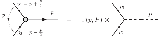
Figure 1: Phenomenological vertex obtained by multiplying a point vertex, representing a structureless particle, by a vertex function (or form factors).

The function $\Gamma$, which is called the 3-point vertex function, can be chosen in different ways. Two simple Ansätze are commonly used in the context of BSE. We consider both. They correspond to two extreme choices at large distances: a dipolar form which decreases gently with its argument, and a gaussian form:

$$\begin{split}\Gamma_{0}(p,P)=\frac{N}{(1-\frac{p^{2}}{\Lambda^{2}})^{2}}\text{ and }\Gamma_{0}(p,P)=Ne^{\frac{p^{2}}{\Lambda^{2}}},\end{split}$$ (2)

both with a free size parameter $\Lambda$. As $\Gamma(p,P)$ in principle depends on $p$ and $P$, we may shift the variable and use $p^{2}-\frac{(p.P)^{2}}{M^{2}}$ instead of $p^{2}$ which has the advantage of reducing to $-|\vec{p}|^{2}$ in the rest frame of the bound state. We refer to it as the vertex function with shifted argument. In the latter cases, we have –in that frame–,

$$\begin{split}\Gamma(p,P)=\frac{N}{(1+\frac{|\vec{p}|^{2}}{\Lambda^{2}})^{2}}\text{ and }\Gamma(p,P)=Ne^{\frac{-|\vec{p}|^{2}}{\Lambda^{2}}}.\end{split}$$ (3)

2.2 Excited states

As is well-known, the number of nodes in the wave function, in whatever space, increases with the principal quantum number $n$. This simple feature can be used to differentiate between $1S$ and $2S$ states.

We thus have simply to determine the position of the node of the wave function in momentum space. To what concerns the vertex function, working in the meson rest frame, the node comes through a prefactor, $1-\frac{|\vec{p}|}{a_{node}}$, which multiplies the vertex function for the $1S$ state. Explicitly, $\Gamma_{2S}(p,P)$, for a node $a_{node}$, reads

$$\begin{split}N^{\prime}\left(1-\frac{|\vec{p}|}{a_{node}}\right)\frac{1}{(1+\frac{|\vec{p}|^{2}}{\Lambda^{2}})^{2}}\text{ and }N^{\prime}\left(1-\frac{|\vec{p}|}{a_{node}}\right)e^{\frac{-|\vec{p}|^{2}}{\Lambda^{2}}}.\end{split}$$ (4)

In order to determine the node position in momentum space, we can use two methods. The first is to fix $a_{node}$ from its known value in position space, e.g. from potential studies, and to Fourier-transform the vertex function. In the case of a gaussian form, this can be carried out analytically.

The second method is to impose the following relation between the $1S$ and $2S$ vertex functions:

$$\begin{split}\int|\vec{p}|^{2}d|\vec{p}|e^{\frac{-|\vec{p}|^{2}}{\Lambda^{2}}}\left(1-\frac{|\vec{p}|}{a_{node}}\right)e^{\frac{-|\vec{p}|^{2}}{\Lambda^{2}}}=0.\end{split}$$ (5)

The two methods give compatible results.

3 Normalising: the leptonic decay width

The width in terms of the decay amplitude $\cal M$, is given by

$$\begin{split}\Gamma_{\ell\ell}=\frac{1}{2M}\frac{1}{(4\pi^{2})}\int\left|\bar{\cal M}\right|^{2}d_{2}(PS),\end{split}$$ (6)

where $d_{2}(PS)$ is the two-particle phase space barger .

The amplitude is obtained as usual through Feynman rules, for which we use our vertex function at the meson-quark-antiquark vertex. At leading order, the square of the amplitude is obtained from the cut-diagram drawn in Fig. 2.

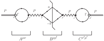
Figure 2: Feynman diagram for ${}^{3}S_{1}\to\ell\bar{\ell}$.

In terms of the sub-amplitudes $A^{\mu\nu}$, $B^{\mu\nu}$ and $C^{\mu\nu}$ defined in Fig. 2, we have:

$$\begin{split}\int\left|\bar{\cal M}\right|^{2}d_{2}(PS)=\frac{1}{3}\Delta_{\mu\mu^{\prime}}A^{\mu\nu}\left(\frac{-ig_{\nu\rho}}{M^{2}}\right)B^{\rho\rho^{\prime}}(\frac{-ig_{\rho^{\prime}\nu^{\prime}}}{M^{2}})C^{\nu^{\prime}\mu^{\prime}},\end{split}$$ (7)

where the factor $\Delta_{\mu\nu}=(g_{\mu\nu}-\frac{P_{\mu}P_{\nu^{\prime}}}{M^{2}})=\sum_{i}\varepsilon_{i,\mu}\varepsilon^{\star}_{i,\mu^{\prime}}$ results from the sum over polarisations of the meson and the factor $\frac{1}{3}$ accounts for the averaging on these initial polarisations.

3.1 Sub-amplitude calculation

To what concerns the sub-amplitude $B^{\rho\rho^{\prime}}$, from the Feynman rules, and after integration on the two-particle phase space, we have

$$\begin{split}B^{\rho\rho^{\prime}}=&(ie)^{2}\left[\pi M^{2}g^{\rho\rho^{\prime}}-8\frac{\pi M^{2}}{24}\left(g^{\rho\rho^{\prime}}+2\frac{P^{\rho}P^{\rho^{\prime}}}{M^{2}}\right)\right]=(ie)^{2}\frac{2\pi}{3}M^{2}\underbrace{\left[g^{\rho\rho^{\prime}}-\frac{P^{\rho}P^{\rho^{\prime}}}{M^{2}}\right]}_{\Delta^{\rho\rho^{\prime}}}.\end{split}$$ (8)

For $A^{\mu\nu}$, from the Feynman rules and using the vertex functions discussed above, we have (see Fig. 3)

$$\begin{split}iA^{\mu\nu}&=-3e_{Q}\int\!\frac{d^{4}k}{(2\pi)^{4}}{\rm Tr}\left((i\Gamma(k,P)\gamma^{\mu})\frac{i(k\!\!\!\!\!/-\frac{1}{2}P\!\!\!\!\!/+m)}{(k-\frac{P}{2})^{2}-m^{2}+i\varepsilon}(ie\gamma^{\nu})\frac{i(k\!\!\!\!\!/+\frac{1}{2}P\!\!\!\!\!/+m)}{(k+\frac{P}{2})^{2}-m^{2}+i\varepsilon}\right)\\ &=-3e_{Q}\int\!\frac{d^{4}k}{(2\pi)^{4}}\Gamma(k,P)\frac{g^{\mu\nu}(M^{2}+4m^{2}-4k^{2})+8k^{\mu}k^{\nu}-2P^{\mu}P^{\nu}}{((k-\frac{P}{2})^{2}-m^{2}+i\varepsilon)((k+\frac{P}{2})^{2}-m^{2}+i\varepsilon)},\end{split}$$ (9)

$e_{Q}$ is the heavy quark charge, $-1$ comes for the fermionic loop, $3$ is the colour factor.

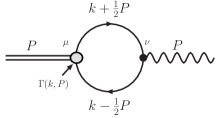
Figure 3: Feynman diagram for ${}^{3}S_{1}\to\gamma^{\star}$.

We can easily motivate our choice of the argument of the vertex function, beside its simple relation with that of wave functions. Its main virtue is to regularise the integration in all spatial directions. In the meson rest frame, the $k^{0}$ integral can be done by standard residue techniques, and the remaining $\vec{k}$ integral is guaranteed to converge. If one uses $k^{2}$ instead of $|\vec{k}|^{2}$ as an argument, it is possible to show that along the light cone, one obtains logarithmic divergences, which would presumably need to be renormalised. Besides, the $k^{0}$ integral then also becomes dependent on the singularity structure of the vertex function. These two reasons make us prefer the shifted vertex in our calculation.

A notable simplification can be obtained by guessing the tensorial form of $A^{\mu\nu}$. Indeed, current conservation (gauge invariance) for the photon can be expressed as:

$$\begin{split}A^{\mu\nu}P_{\nu}=0.\end{split}$$ (10)

It is equivalent to

$$\begin{split}iA^{\mu\nu}=iF(g^{\mu\nu}-\frac{P^{\mu}P^{\nu}}{M^{2}})=iF\Delta^{\mu\nu},\end{split}$$ (11)

the coefficient $F$ being $\frac{A^{\mu}_{\ \mu}}{3}$ since $A^{\mu}_{\ \mu}=A^{\mu\nu}g_{\nu\mu}=3F$. This assumption can be easily verified in the bound-state rest frame $P=(M,0,0,0)$ for which Eq. (10) reduces to $A^{\mu 0}M=0\Rightarrow A^{\mu 0}=0$. We shall check this at the end of this calculation.

It is therefore sufficient to compute the following quantity, where we set $|\vec{k}|^{2}\equiv K^{2}$ and define $\Gamma(-K^{2})=\Gamma(k,P)$,

$$\begin{split}iA^{\mu}_{\ \mu}=-3e_{Q}&\int_{0}^{\infty}4\pi K^{2}dK\Gamma(-K^{2})\times\\ &\int_{-\infty}^{\infty}\frac{dk_{0}}{(2\pi)^{4}}\frac{4(-2(k^{2}-\frac{M^{2}}{4})+4m^{2})}{((k-\frac{P}{2})^{2}-m^{2}+i\varepsilon)((k+\frac{P}{2})^{2}-m^{2}+i\varepsilon))}.\end{split}$$ (12)

Let us first integrate on $k_{0}$ by residues. Defining $E=\sqrt{K^{2}+m^{2}}$, we determine the position of the pole on $k_{0}$ (still in the bound-state rest frame) as

$$\begin{split}&(k\pm\frac{P}{2})^{2}-m^{2}+i\varepsilon=(k_{0}\pm\frac{M}{2})^{2}-E^{2}+i\varepsilon.\end{split}$$ (13)

To calculate the integral on $k_{0}$, we choose the contour as drawn in Fig. 4. Two poles $-E-\frac{M}{2}$ and $-E+\frac{M}{2}$ are located in the upper half-plane and the two others in the lower half-plane. We shall therefore have two residues to consider. The contribution of the contour ${\cal C}_{R}$ vanishes as $R$ tends to $\infty$.

$$\begin{split}&iA^{\mu}_{\ \mu}=\frac{-3e_{Q}}{\pi^{3}}\int_{0}^{\infty}K^{2}dK\Gamma(-K^{2})\times\\ &2i\pi\left[\frac{-2(-E-\frac{M}{2})^{2}+\frac{M^{2}}{2}+2E^{2}+2m^{2}}{(-2E)(-M)(-2(E+\frac{M}{2}))}\right.+\left.\frac{-2(-E+\frac{M}{2})^{2}+\frac{M^{2}}{2}+2E^{2}+2m^{2}}{M(-2(E-\frac{M}{2}))(-2E)}\right]\\ &=\frac{-3e_{Q}}{\pi^{3}}\int_{0}^{\infty}K^{2}dK\Gamma(-K^{2})\frac{2i\pi}{4ME}\underbrace{\left[-\frac{2EM+2m^{2}}{E+\frac{M}{2}}+\frac{2EM+2m^{2}}{E-\frac{M}{2}}\right]}_{\frac{M(4E^{2}+2m^{2})}{E^{2}-\frac{M^{2}}{4}}}.\end{split}$$ (14)

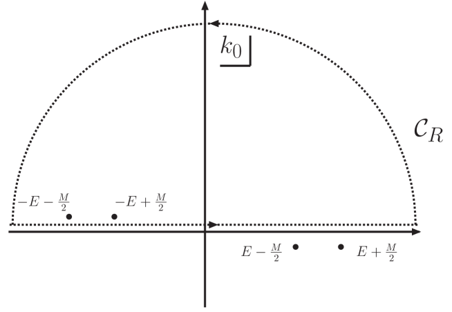
Figure 4: Illustration of the contour chosen to integrate on $k_{0}$.

The procedure is correct only if the poles of the upper-plane are on the left side and those of the lower-plane are on the right.

This crossing would first occur between the points $-E+\frac{M}{2}$ and $E-\frac{M}{2}$. Solving for $E$, we have:

$$\begin{split}-E+\frac{M}{2}=E-\frac{M}{2}&\Rightarrow\frac{M^{2}}{4}-m^{2}=K^{2}>0.\end{split}$$ (15)

The crossing is therefore impossible when $M<2m$. Therefore, to get a coherent description of all charmonia (resp. bottomonia) below the open charm (resp. beauty) threshold, we shall set the quark mass high enough to avoid crossing for all of these. This sets $m_{c}$ to 1.87 GeV ($m_{D}$) and $m_{b}$ to 5.28 GeV ($m_{B}$). Considering the variety of results obtained from potential models, this seems to be a sensible choice.

Putting it all together, we get

$$\begin{split}A^{\mu}_{\ \mu}=\frac{-3e_{Q}}{\pi^{2}}\int_{0}^{\infty}dK\frac{K^{2}\Gamma(-K^{2})}{\sqrt{K^{2}+m^{2}}}\frac{(2K^{2}+3m^{2})}{(K^{2}+m^{2}-\frac{M^{2}}{4})}.\end{split}$$ (16)

One is left with the integration on $K$ for which we define the integral $I$ depending on the vertex function whose normalisation is pulled off,

$$\begin{split}I(\Lambda,M,m)\equiv\int_{0}^{\infty}\frac{dKK^{2}}{\sqrt{K^{2}+m^{2}}}\frac{\Gamma(-K^{2})}{N}\frac{(2K^{2}+3m^{2})}{(K^{2}+m^{2}-\frac{M^{2}}{4})},\end{split}$$ (17)

$I$ is a function of $\Lambda$ through the vertex function $\Gamma(-K^{2})$ and is not in general computable analytically. In the following we shall leave it as is and express $A^{\mu\nu}$ as:

$$\begin{split}A^{\mu}_{\ \mu}=\frac{-3e_{Q}}{\pi^{2}}NI(\Lambda,M,m)\Rightarrow A^{\mu\nu}=\frac{-e_{Q}}{\pi^{2}}NI(\Lambda,M,m)\Delta^{\mu\nu}.\end{split}$$ (18)

Finally, to what concerns the sub-amplitude $C$, we simply have

$$\begin{split}C^{\nu^{\prime}\mu^{\prime}}=(A^{\nu^{\prime}\mu^{\prime}})^{\dagger}=A^{\nu^{\prime}\mu^{\prime}}.\end{split}$$ (19)

3.2 Results

Now that all quantities in Eq. (7) are determined, we can combine them. Hence, we obtain:

$$\begin{split}&\int\left|\bar{\cal M}\right|^{2}d_{2}(PS)=\frac{\Delta_{\mu\mu^{\prime}}}{3}\frac{-1}{M^{4}}\left(\frac{e_{Q}}{\pi^{2}}NI(\Lambda,M,m)\right)^{2}\left((ie)^{2}\frac{2\pi}{3}M^{2}\right)\Delta^{\mu\nu}g_{\nu\rho}\Delta^{\rho\rho^{\prime}}g_{\rho^{\prime}\nu^{\prime}}\Delta^{\nu^{\prime}\mu^{\prime}}\end{split}$$ (20)

The leptonic decay width eventually reads from Eq. (6):

$$\begin{split}\Gamma_{\ell\ell}=N^{2}\frac{e^{2}}{12\pi M^{3}}\left(\frac{e_{Q}}{\pi^{2}}I(\Lambda,M,m)\right)^{2}.\end{split}$$ (21)

3.2.1 Numerical results

The value of $N$ is in practice obtained by replacing $\Gamma_{\ell\ell}$ by its measured value, $e_{Q}$ by $\frac{2e}{3}$ for $c$ quark and $\frac{-e}{3}$ for $b$ quark and, finally, by introducing the value obtained for $I$ for the chosen value of $\Lambda$. We sketch in Fig. 5 and Fig. 6 some plots of $N$ for the $J/\psi$ and for the $\Upsilon(1S)$ to show its dependence on $\Lambda$ and $m_{Q}$ and the value it actually takes.

Figure 5: Normalisation for a dipolar (resp. gaussian) form for $J/\psi$ as a function of $\Lambda$: right (resp. left ).

Figure 6: Normalisation for a dipolar (resp. gaussian) form for $\Upsilon(1S)$ as a function of $\Lambda$: right (resp. left ).

$m_{c}$ (GeV)	Vertex functions
1.6 1.7 1.87	Gaussian Dipole $N$ $\Lambda$ (GeV) 1.59 2.34 2.28 2.08 3.31 1.97 $N$ $\Lambda$ (GeV) 1.33 2.87 1.87 2.54 2.76 2.31

Table 1: Set of values for $m_{c}$, $\Lambda$ and $N$ obtained for the $J/\psi$ within BSE approach costa .

We have chosen the range of size of the mesons, or $\Lambda$, following BSE studies costa and other phenomenological models Ivanov:2000aj ; Ivanov:2003ge , where the commonly accepted values for the $J/\psi$ are from around $1$ to $2.4$ GeV, and for the $\Upsilon(1S)$ from around $3.0$ to $6.5$ GeV. For illustration, we put in Tab. 1 several values of $\Lambda$ obtained with BSE costa , accompanied with the vertex-function normalisation.

3.2.2 Result for $\psi^{\prime}$ and implication for the $\rho$-$\pi$ puzzle

To what concerns the $\psi^{\prime}$, we give the results for $\Lambda$=1.8 GeV, $m_{c}=1.87$ GeV and a gaussian vertex function (see Fig. 7). The normalisation $N^{\prime}$ diverges for $a_{node}\simeq 1.35$ GeV. This comes from the cancellation of the leptonic decay width for this value of $a_{node}$.

Figure 7: $N^{\prime}$ for the $\psi^{\prime}$ as a function of $a_{node}$.

This cancellation can be traced back to the integrand of $I$ (see Eq. (17)), which we note $\frac{dI}{dK}$ (see Fig. 8). The cancellation of the positive contribution by the negative one therefore occurs in this case for $a_{node}=1.35$ GeV.

Figure 8: Evolution of the integrand in $I$ as a function of $K$ and for three values of $a_{node}$ in the $\psi^{\prime}$ case.

The constraint for the node position Eq. (5) gives $a_{node}=1.46$ GeV for these values of $\Lambda$ and $m_{c}$. For this value of $a_{node}$, the normalisation $N^{\prime}$ is 16.36. This was the value that we have retained for the numerical applications of these .

In the case of the hadronic decay $\psi^{\prime}\to\rho\pi$, we expect it to proceed via an off-shell $\omega$ (see Fig. 9). The integral $I$ involving the $\psi^{\prime}$ vertex function will be slightly different and might be, for the same value of $a_{node}$, drastically suppressed.

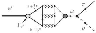
Figure 9: Possible decay of a $\psi^{\prime}$ into a $\rho$ - $\pi$ pair via an off-shell $\omega$.

We can therefore expect a severe suppression of the decay amplitude compared to the nodeless, i.e. $J/\psi$, case. This suppression could in turn explains the $\rho-\pi$ puzzle, namely that the measured ratio $\frac{\Gamma(\psi^{\prime}\to\rho\pi)}{\Gamma(J/\psi\to\rho\pi)}$ is not of the order of 15 % (expected from the leptonic decays) but rather smaller than 1%.

4 Conclusion

We have explained our approach to describe on a phenomenological basis the internal dynamics of heavy quarkonia in the context of a Feynman-diagram calculation. We have also provided a way to represent the distinct features of $2S$ states, like the $\psi^{\prime}$. We have seen that a simple but robust constraint on the vertex functions for $1S$-states could be achieved by imposing that their normalisation reproduces the leptonic decay width, through a simple leading order calculation.

An interesting simplification can be also obtained by shifting the argument of the vertex function, namely the relative momentum of the quark inside the quarkonium, into a quantity that reduce to the tri-dimensional relative momentum in the meson rest frame. This enable us to work out analytically, for whatever vertex function, the integration on $k_{0}$.

Furthermore, we have shown that the leptonic decay width was very dependent on the node position, which, incidentally, is not a completely constrained parameter. This induces the same effects on the normalisation (see Fig. 7). This has consequences on production processes where our approach to describe internal dynamics of heavy quarkonia can be applied (see these ; Lansberg:2005pc ; article2 ). It should be interesting to see whether this happens for other excited states. Finally, we suggest that this feature typical of radially excited states could be the awaited explanation for the longtstanding $\rho-\pi$ puzzle.

References

- (1) J. P. Lansberg, Quarkonium Production at High-Energy Hadron Colliders, Ph.D. Thesis, Liège University, Belgium. ISBN: 2-87456-004-9 [arXiv:hep-ph/0507175].
- (2) J. P. Lansberg, J. R. Cudell and Yu. L. Kalinovsky, arXiv:hep-ph/0507060.
- (3) J. R. Cudell, Yu. L. Kalinovsky and J. P. Lansberg, (in preparation).
- (4) F. Abe et al. [CDF Collaboration], Phys. Rev. Lett. 79 (1997) 572.
- (5) F. Abe et al. [CDF Collaboration], Phys. Rev. Lett. 79 (1997) 578.
- (6) T. Affolder et al. [CDF Collaboration], Phys. Rev. Lett. 85 (2000) 2886 [arXiv:hep-ex/0004027].
- (7) D. Acosta et al. [CDF Collaboration], Phys. Rev. Lett. 88 (2002) 161802.
- (8) S. S. Adler et al. [PHENIX Collaboration], Phys. Rev. Lett. 92 (2004) 051802 [arXiv:hep-ex/0307019].
- (9) E. E. Salpeter and H. A. Bethe, Phys. Rev. 84 (1951) 1232.
- (10) P. Maris and C. D. Roberts, Int. J. Mod. Phys. E 12 (2003) 297 [arXiv:nucl-th/0301049].
- (11) C. J. Burden, L. Qian, C. D. Roberts, P. C. Tandy and M. J. Thomson, Phys. Rev. C 55 (1997) 2649 [arXiv:nucl-th/9605027].
- (12) M. A. Ivanov, Y. L. Kalinovsky and C. D. Roberts, Phys. Rev. D 60 (1999) 034018 [arXiv:nucl-th/9812063].
- (13) M. A. Ivanov, J. G. Korner and P. Santorelli, Phys. Rev. D 63 (2001) 074010 [arXiv:hep-ph/0007169].
- (14) M. A. Ivanov, J. G. Korner and P. Santorelli, Phys. Rev. D 70 (2004) 014005 [arXiv:hep-ph/0311300].
- (15) V.D. Barger and R.J.N. Philips, Collider Physics, Addison-Wesley, Menlo Park, 1987.
- (16) P. Costa (private communication).