Flipped SU(5), see–saw scale physics and degenerate vacua

Abstract

We investigate the requirement of the existence of two degenerate vacua of the effective potential as a function of the Weinberg–Salam Higgs scalar field norm, as suggested by the multiple point principle, in an extension of the Standard Model including see–saw scale physics. Results are presented from an investigation of an extension of the Standard Model to the gauge symmetry group $SU(3)_{C}\times SU(2)_{L}\times U(1)^{\prime}\times\tilde{U}(1)$, where two groups $U(1)^{\prime}$ and $\tilde{U}(1)$ originate at the see–saw scale $M_{SS}$, when heavy (right–handed) neutrinos appear. The consequent unification of the group $SU(3)_{C}\times SU(2)_{L}\times U(1)^{\prime}$ into the flipped $SU(5)$ at the GUT scale leads to the group $SU(5)\times\tilde{U}(1)$. We assume the position of the second minimum of the effective potential coincides with the fundamental scale, here taken to be the GUT scale. We solve the renormalization group equations in the one–loop approximation and obtain a top–quark mass of $171\pm 3$ GeV and a Higgs mass of $129\pm 4$ GeV, in the case when the Yukawa couplings of the neutrinos are less than half that of the top quark at the GUT scale.

For some time [1, 2] we have sought to derive the values of Standard Model (SM) parameters from what we call the Multiple Point Principle (MPP), according to which there are several vacua all having exceedingly small cosmological constants like the vacuum in which we live now. But we have no guarantee for how far the SM will work up the energy scale. To investigate the influence of new physics – especially the see–saw neutrino mass producing physics [3] – at higher scales on our predictions from MPP, such as the top–quark mass or the Higgs mass, we shall here investigate a non–supersymmetric flipped $SU(5)$ extension of the SM broken though not in the normally suggested way by a decuplet (or in SUSY versions even a couple of conjugate decuplets). Rather we let the flipped $SU(5)$, which is $SU(5)\times\tilde{U}(1)$, break stepwise, firstly highest in energy scale at the unifying scale $M_{GUT}$ by an adjoint Higgs field down to $SU(3)_{C}\times SU(2)_{L}\times U(1)^{\prime}\times\tilde{U}(1)$ and next at a lower see–saw scale $M_{SS}$ down to the SM group $SU(3)_{C}\times SU(2)_{L}\times U_{Y}(1)$, say by a Higgs field $S$ which belongs to a $\underline{50}$ representation of $SU(5)$. It is our philosophy not to take the details too seriously but rather think of the flipped $SU(5)$ as a typical representative model with new physics, which we can use to estimate the magnitude of the deviations caused to the MPP–predictions.

The specific stepwise breaking used in the present article is taken in order to have a see–saw scale as a separate scale which can be varied. In this respect we do not use the advertised benefits of the usual flipped $SU(5)$ [3, 4, 5], which does not use an adjoint Higgs field but rather a decuplet Higgs as favoured by superstring theory.

In flipped $SU(5)$, the quarks and leptons are in the $\underline{1},\underline{\bar{5}},\underline{10}$ representations, but with assignments and electric charges ‘flipped’ relative to conventional $SU(5)$. In either standard or ‘flipped’ $SU(5)$ [6, 7, 8] a single generation of 16 matter fields, including a singlet right–handed neutrino, can be accommodated by a set of $\underline{1},\underline{\bar{5}},\underline{10}$ representations. However, the difference between the flipped and conventional versions of $SU(5)$ is in the way in which the 16 matter fields of each generation are embedded in these representations. Flipped $SU(5)$ received its name from the exchanges in the assignments of the fields: up–like and down–like fields are exchanged, as are electron–like with neutrino–like, as well as their anti–particle partners. The particle content of the flipped $SU(5)\times{\tilde{U}}(1)$ model used here is as follows

• three generations of matter fields:

  $$F=\left(\underline{10},\,\frac{1}{2\sqrt{10}}\right),\qquad{\bar{f}}_{i}=\left(\underline{\bar{5}},\,-\frac{3}{2\sqrt{10}}\right),\qquad l_{i}^{c}=\left(\underline{1},\,\frac{5}{2\sqrt{10}}\right),\qquad(i=1,2,3),$$ (1)

• a five–dimensional (Weinberg–Salam) Higgs to break $SU(2)_{L}\times U(1)_{Y}$:

  $$\phi=\left(\underline{5},\,-\frac{1}{\sqrt{10}}\right),$$ (2)

• an adjoint 24–dimensional Higgs to break $SU(5)\times\tilde{U}(1)\to SU(3)_{C}\times SU(2)_{L}\times U(1)^{\prime}\times\tilde{U}(1):$

  $$A=(\underline{24},\,0),$$ (3)

• a Higgs field $S$ to break $SU(3)_{C}\times SU(2)_{L}\times U(1)^{\prime}\times\tilde{U}(1)\to SU(3)_{C}\times SU(2)_{L}\times U(1)_{Y}$ at the see–saw scale, with the following $U(1)^{\prime}\times\tilde{U}(1)$ quantum numbers:

  $$Q^{\prime}_{S}=2\sqrt{\frac{3}{5}},\qquad\tilde{Q}_{S}=\sqrt{\frac{1}{10}}.$$ (4)

We note that we have chosen to normalise all the flipped $SU(5)$ generators $T_{a}$ such that the trace of $T_{a}^{2}$ over the 16 fermions in a single quark–lepton generation is given by $Tr_{16}(T_{a}^{2})=2$.

We do not attempt here to solve the fermion mass problem, which would need extra new physics [9] at, say, the GUT scale. However phenomenologically we know that, apart from the top quark, the Yukawa couplings of charged fermions can be neglected. Unfortunately, we do not have direct information about the Yukawa couplings of the neutrinos. In a naive minimal flipped $SU(5)$ model one might expect that the Dirac neutrino mass matrix would be equal to the up quark mass matrix. But the see–saw mechanism would then almost inevitably give an unrealistically strong hierarchy of light neutrino masses. Since we cannot extract reliable values for the neutrino Yukawa couplings, we allow the possibility that one of them $y_{\nu}$ might be as large as the top quark Yukawa coupling $h$ and introduce the parameter $p$ giving their ratio at the GUT scale $M_{GUT}$:

$$y_{\nu}(M_{GUT})=p\cdot h(M_{GUT}),$$ (5)

where $0\leq p\leq 1$.

The renormalization group equations (RGEs) are:

$$\frac{dg_{i}}{dt}=\beta_{g_{i}},\qquad\frac{dh}{dt}=\beta_{h},\qquad\frac{d\lambda}{dt}=\beta_{\lambda},\qquad\frac{dy_{\nu}}{dt}=\beta_{y_{\nu}},$$ (6)

where $t=\ln(\mu/M)=\ln(\phi/M)$ is the evolution variable, $\mu$ is the energy scale, $M$ is the renormalization mass scale and $\phi$ is the Weinberg–Salam Higgs scalar field. Its vacuum expectation value (VEV) is:

$$<\phi>=\frac{1}{\sqrt{2}}\left(\begin{array}[]{c}0\\ {\it v}\end{array}\right),\qquad{\mbox{with}}\qquad v\approx 246\ \mbox{GeV}.$$ (7)

The gauge couplings $g_{i}=(g_{1},g_{2},g_{3})$ correspond to the $U(1)$, $SU(2)_{L}$ and $SU(3)_{C}$ groups of the SM, and $\lambda$ is the Weinberg–Salam Higgs field self–interaction coupling constant. We neglect the Yukawa couplings of all the other fermions. Also we neglect interactions of the form $\phi^{2}S^{2}$ between the Higgs fields.

In the Weinberg–Salam theory the tree level masses of the gauge bosons $W$ and $Z$, the top quark and the physical Higgs boson $H$ are expressed in terms of the VEV parameter $v$:

$$M_{W}^{2}=\frac{1}{4}g^{2}v^{2},\qquad M_{Z}^{2}=\frac{1}{4}\left(g^{2}+g^{\prime 2}\right)v^{2},\qquad m_{t}=\frac{1}{\sqrt{2}}hv,\qquad m_{H}^{2}=\lambda v^{2},$$ (8)

where $g^{\prime}\equiv g_{Y}=\sqrt{(3/5)}\,g_{1}$, $g\equiv g_{2}$. The one–loop $\beta$–functions in the SM are:

$$16\pi^{2}\beta_{g_{1}}^{(1)}=\frac{41}{10}g_{1}^{3},\qquad 16\pi^{2}\beta_{g_{2}}^{(1)}=-\frac{19}{6}g_{2}^{3},\qquad 16\pi^{2}\beta_{g_{3}}^{(1)}=-7g_{3}^{3},$$ (9)

$$16\pi^{2}\beta_{h}^{(1)}=h\left(\frac{9}{2}h^{2}-8g_{3}^{2}-\frac{9}{4}g_{2}^{2}-\frac{17}{20}g_{1}^{2}\right),$$ (10)

$$16\pi^{2}\beta_{\lambda}^{(1)}=12\lambda^{2}+\lambda\left(12h^{2}-9g_{2}^{2}-\frac{9}{5}g_{1}^{2}\right)+\frac{27}{100}g_{1}^{4}+\frac{9}{10}g_{1}^{2}g_{2}^{2}+\frac{9}{4}g_{2}^{4}-12h^{4}.$$ (11)

These equations are valid up to the see–saw scale $M_{SS}$.

In the region from $M_{SS}$ to $M_{GUT}$ we have a new type of symmetry $SU(3)_{C}\times SU(2)_{L}\times U(1)^{\prime}\times\tilde{U}(1)$ with the following one–loop $\beta$–functions for the corresponding RGEs similar to (6):

$$16\pi^{2}\beta_{{g^{\prime}}_{1}}^{(1)}=\frac{45}{10}{g^{\prime}}_{1}^{3},\qquad 16\pi^{2}\beta_{\tilde{g}_{1}}^{(1)}=\frac{41}{10}{\tilde{g}_{1}}^{3},\qquad 16\pi^{2}\beta_{g_{2}}^{(1)}=-\frac{19}{6}g_{2}^{3},\qquad 16\pi^{2}\beta_{g_{3}}^{(1)}=-7g_{3}^{3},$$ (12)

$$16\pi^{2}\beta_{h}^{(1)}=h\left(\frac{9}{2}h^{2}-8g_{3}^{2}-\frac{9}{4}g_{2}^{2}-\frac{1}{4}{g^{\prime}}_{1}^{2}-\frac{3}{4}{\tilde{g}}_{1}^{2}\right),$$ (13)

$$16\pi^{2}\beta_{y_{\nu}}^{(1)}=y_{\nu}\left(\frac{5}{2}y_{\nu}^{2}-\frac{9}{4}g_{2}^{2}-\frac{3}{4}{g^{\prime}}_{1}^{2}-\frac{1}{4}{\tilde{g}}_{1}^{2}\right),$$ (14)

$$16\pi^{2}\beta_{\lambda}^{(1)} = 12\lambda^{2}+\lambda\left[12h^{2}+4y_{\nu}^{2}-9g_{2}^{2}-\frac{9}{5}\left({g^{\prime}}_{1}^{2}+\frac{2}{3}{\tilde{g}}_{1}^{2}\right)\right]+\frac{27}{100}\left({g^{\prime}}_{1}^{2}+\frac{2}{3}{\tilde{g}}_{1}^{2}\right)^{2}$$ (15)

$$+\frac{9}{10}\left({g^{\prime}}_{1}^{2}+\frac{2}{3}{\tilde{g}}_{1}^{2}\right)g_{2}^{2}+\frac{9}{4}g_{2}^{4}-12h^{4}-4y_{\nu}^{4}.$$

Here we neglected small couplings.

Following the idea of Refs. [1, 2], we assume that in the present model the fundamental scale $M_{fund}$ coincides with the GUT scale $M_{GUT}$ for $SU(5)\times{\tilde{U}}(1)$. This idea is based on the Multiple Point Principle (MPP) [10] (see also the reviews [11, 12]), according to which several vacuum states with the same energy density exist in Nature. In the pure SM the effective potential for the Weinberg–Salam Higgs field can have two degenerate minima as a function of $|\phi|$:

$$V_{eff}(\phi_{min1}^{2})=V_{eff}(\phi_{min2}^{2})=0,$$ (16)

$$V^{\prime}_{eff}(\phi_{min1}^{2})=V^{\prime}_{eff}(\phi_{min2}^{2})=0,$$ (17)

where

$$V^{\prime}(\phi^{2})=\frac{\partial V}{\partial\phi^{2}}.$$ (18)

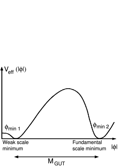
Fig. 1: Fundamental scale vacuum degenerate with usual SM weak scale vacuum.

The first minimum is the standard “Weak scale minimum”, and the second one is the non–standard “Fundamental scale minimum” as shown in Fig. 1. In the present model the assumption is that the second minimum of the effective potential coincides with the GUT–scale $\phi_{min2}=M_{GUT}$.

As discussed in Ref. [1], for large values of the Higgs field $\phi^{2}\gg v^{2}$ the degeneracy conditions (16) and (17) lead to the following requirements:

$$\lambda(\phi_{min2})=0,\qquad\beta_{\lambda}(\phi_{min2},\lambda=0)=0.$$ (19)

Taking $\phi_{min2}\sim M_{Planck}$ and using the two–loop RGEs, the following MPP predictions were obtained in the pure SM for the top quark and Weinberg–Salam Higgs particle masses [1, 13]:

$$M_{t}=173\pm 5\ \mbox{GeV},\qquad M_{H}=135\pm 9\ \mbox{GeV}.$$ (20)

We note that the present experimental value [14] of the top quark mass is:

$$M_{t}=172.7\pm 2.7.$$ (21)

When solving the RGEs (12–15) we use the MPP conditions (19) at the GUT scale, which in our case determine the top quark Yukawa coupling at the GUT scale in terms of the $SU(2)_{L}\times U(1)^{\prime}\times\tilde{U}(1)$ gauge couplings at the GUT scale and the parameter $p$:

$$4(3+p^{4})h^{4}=\frac{27}{100}\left({g^{\prime}}_{1}^{2}+\frac{2}{3}{\tilde{g}}_{1}^{2}\right)^{2}+\frac{9}{10}\left({g^{\prime}}_{1}^{2}+\frac{2}{3}{\tilde{g}}_{1}^{2}\right)g_{2}^{2}+\frac{9}{4}g_{2}^{4}.$$ (22)

By considering the joint solution of the RGEs (9–15), we estimate corrections to the MPP predictions for $M_{t}$ and $M_{H}$, due to the new see–saw scale physics.

Starting from the Particle Data Group [15], the phenomenological input to our calculations are the $Z^{0}$ mass:

$$M_{Z}=91.1876\pm 0.0021\ {\mbox{GeV}},$$ (23)

the inverse electromagnetic fine structure constant and the square of the sine of the weak angle in the $\overline{\rm{MS}}$–scheme:

$${\hat{\alpha}}^{-1}(M_{Z})=127.906\pm 0.019,\qquad{\hat{s}}^{2}(M_{Z})=0.23120\pm 0.00015,$$ (24)

and the QCD fine structure constant:

$$\alpha_{3}(M_{Z})=0.119\pm 0.002.$$ (25)

The only other input to our calculation is the value of the parameter $p$.

It is well–known that the running of all the gauge coupling constants in the SM is well described by the one–loop approximation. For $M_{t}\leq\mu\leq M_{SS}$ we have the following evolutions for the inverses of the fine structure constants $\alpha_{i}=g_{i}^{2}/{4\pi}$, $(i=1,2,3)$, which are revised using the updated experimental results [15]:

$$\alpha_{1}^{-1}(t)=58.65\pm 0.02-\frac{41}{20\pi}t,$$ (26)

$$\alpha_{2}^{-1}(t)=29.95\pm 0.02+\frac{19}{12\pi}t,$$ (27)

$$\alpha_{3}^{-1}(t)=9.17\pm 0.20+\frac{7}{2\pi}t,$$ (28)

where $t=\ln(\mu/{M_{t}}).$ The gauge coupling constant evolutions (26–28) are shown in Fig. 2, where $x=\log_{10}\mu$ (GeV) and $t=x\ln 10-\ln{M_{t}}$. The evolutions (27) and (28) are valid up to the GUT scale for $M_{t}\leq\mu\leq M_{GUT}$. But Eq. (26) works only up to the see–saw scale. At the scale $M_{SS}$ the two $U(1)$ groups – $U(1)^{\prime}$ and $\tilde{U}(1)$ – become active and give, instead of Eq. (26), the following new fine structure constant evolutions:

$${\alpha^{\prime}}_{1}^{-1}(t)={\alpha^{\prime}}_{1}^{-1}(M_{SS})-\frac{45}{20\pi}{\tilde{t}},$$ (29)

$${\tilde{\alpha}}_{1}^{-1}(t)={\tilde{\alpha}}_{1}^{-1}(M_{SS})-\frac{41}{20\pi}{\tilde{t}},$$ (30)

which are valid for the interval $M_{SS}\leq\mu\leq M_{GUT}$. In Eq. (30)

$$\tilde{t}=\ln\left(\frac{\mu}{M_{SS}}\right)=t+\ln\left(\frac{M_{t}}{M_{SS}}\right)=x\ln 10-\ln M_{SS}.$$

For convenience we have also considered the evolution of:

$$y_{top}(t)=\alpha_{h}^{-1}(t)=\left(\frac{h^{2}(t)}{4\pi}\right)^{-1}.$$ (31)

The mixture of the two $U(1)$ groups at the see–saw scale leads to the following relation (compare with Refs. [4, 5]):

$$\alpha_{1}^{-1}(M_{SS})=\frac{24}{25}{\tilde{\alpha}}_{1}^{-1}(M_{SS})+\frac{1}{25}{\alpha^{\prime}}_{1}^{-1}(M_{SS}).$$ (32)

At the GUT scale we have the unification $SU(3)_{C}\times SU(2)_{L}\times U(1)^{\prime}\to SU(5)$ giving:

$${\alpha^{\prime}}_{1}(M_{GUT})=\alpha_{2}(M_{GUT})=\alpha_{3}(M_{GUT})=\alpha_{GUT}.$$ (33)

The GUT scale is given by the intersection of the evolutions (27) and (28) for $\alpha_{2}^{-1}(x)$ and $\alpha_{3}^{-1}(x)$.

From Eq. (32), using Eqs. (29), (30) and relations (33), we obtain the following relation:

$$\tilde{\alpha}_{1}^{-1}(M_{GUT})=\frac{25}{24}\alpha_{1}^{-1}(M_{GUT})-\frac{1}{24}\alpha_{GUT}^{-1}-\frac{1}{120\pi}\ln\left(\frac{M_{GUT}}{M_{SS}}\right).$$ (34)

where the RGE for $\alpha_{1}(t)$ has been formally extended to the GUT scale.

We now investigate the dependence of the MPP predictions on the see–saw scale physics, by varying the see–saw scale $M_{SS}$ and the parameter $p$ which determines the neutrino Yukawa coupling $y_{\nu}$. Once $M_{SS}$ and $p$ are fixed, the values of all the gauge couplings can be determined at the GUT scale, where we also have the boundary values (22), (5) and (19) for $h(M_{GUT})$, $y_{\nu}(M_{GUT})$ and $\lambda(M_{GUT})$ respectively. The RGEs (9–15) can then be integrated down from the GUT scale, requiring continuity at the see–saw scale, to the electroweak scale. In this way we determine the running top quark mass $m_{t}(\mu=m_{t})=h(\mu=m_{t})v/\sqrt{2}$ and the Higgs self–coupling $\lambda(m_{t})$. We can then calculate [13, 16] the top quark pole mass $M_{t}$ and the Higgs pole mass $M_{H}$.

We find that our results are highly insensitive to the value of the see–saw scale $M_{SS}$, which is allowed to range from 10 TeV to the GUT scale ($M_{GUT}\sim 10^{17}$ GeV). However, as a consequence of Eq. (22), there is a significant dependence on $p$ for $p\sim 1$. So we present below our results for three values of $p$:

$$p=0\qquad M_{t}=171\pm 3\ \mbox{GeV}\qquad M_{H}=129\pm 4\ \mbox{GeV},$$ (35)

$$p=1/2\qquad M_{t}=169\pm 3\ \mbox{GeV}\qquad M_{H}=128\pm 4\ \mbox{GeV},$$ (36)

$$p=1\qquad M_{t}=164\pm 3\ \mbox{GeV}\qquad M_{H}=118\pm 4\ \mbox{GeV}.$$ (37)

We see that for $p\leq 1/2$, the results are essentially independent of the new see–saw scale physics. Comparing to the pure SM degenerate vacuum based prediction (20), it means that taking the second minimum (assumed degenerate with the present vacuum) down from the Planck to the GUT scale and including the $\beta$–function effects of our flipped $SU(5)$ only shifts the Higgs mass down by 6 GeV, predicting the top quark mass of $171\pm 3$ GeV in agreement with experiment [14]. However for $p=1$ the MPP prediction for the top quark mass is reduced to $164\pm 3$ GeV, which is disfavoured by experiment, although the corresponding Higgs mass of $118\pm 4$ GeV is close to the signal observed by the Aleph group at LEP [17].

Fig. 3 shows an example of the evolutions of $\lambda(x)$ and $y_{top}(x)$ for $M_{t}=171$ GeV, $M_{H}=129$ GeV and $\alpha_{s}(M_{Z})=0.119$, with $p=0$ and $M_{SS}\sim 10^{11}$ GeV. Fig. 2 presents the running of all the fine structure constants for the same experimental parameters.

We intend to estimate the effects of including two–loop contributions in the RGEs and to investigate the effect of varying the position of the second minimum relative to the GUT scale (e.g. up to the Planck scale). However it is already clear that the MPP predictions for the top quark and Higgs masses are rather insensitive to the introduction of new see–saw scale physics associated with neutrino masses, unless one of the neutrino Yukawa couplings is at least similar in magnitude to that of the top quark.

Acknowledgements:  One of the author (LVL) thanks the Institute of Mathematical Sciences, Chennai (India) for hospitality and financial support. CRD thanks Prof. G. Rajasekaran and Prof. U. Sarkar for useful discussions. This work is supported by the Russian Foundation for Basic Research (RFBR), project No. 05–02–17642. CDF would like to acknowledge the hospitality of the Niels Bohr Institute and support from the Niels Bohr Institute Fund and PPARC.

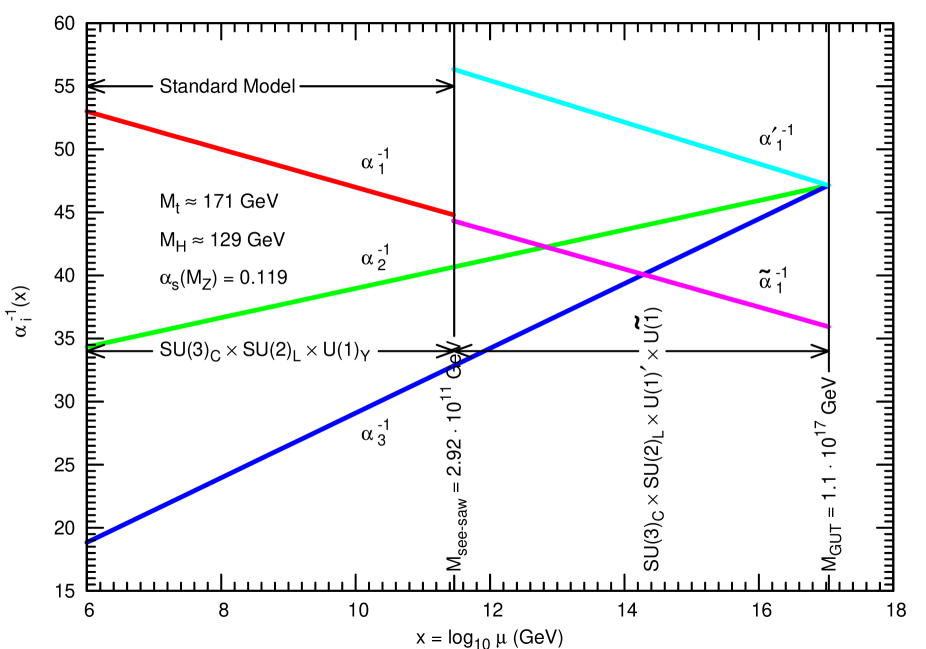
Fig. 2: Evolution of the running inverse fine structure constants, showing the appearance of the $U(1)^{\prime}\times\tilde{U}(1)$ gauge symmetry at the see–saw scale.

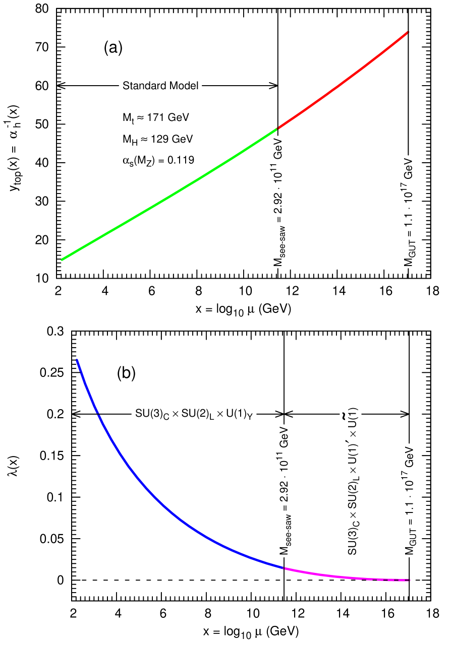
Fig. 3: Evolution of (a) $y_{top}(x)=\alpha^{-1}_{h}(x)=4\pi/h^{2}(x)$ for the top quark and (b) the Weinberg–Salam Higgs self–coupling constant $\lambda(x)$ for the case $p=0$.

References

• [1] C.D. Froggatt, H.B. Nielsen, Phys.Lett. B368, 96 (1996).
• [2] C.D. Froggatt, L.V. Laperashvili and H.B. Nielsen, to appear in Yad.Fiz. 69, 1 (2006); arXiv: hep-ph/0407102.
• [3] T. Yanagida, in Proceedings of the Workshop on Unified Theories and Baryon Number in the Universe, Tsukuba, Japan, 1979, Ed. by A. Sawada and A. Sugamoto, KEK Report No. 79–18, Tsukuba.
M. Gell–Mann, P. Ramond and R. Slansky, in Proceedings of the Supergravity Stony Brook Workshop, New York, 1979, Ed. by P. Van Niewenhuizen and D. Freeman, (North–Holland, Amsterdam, 1979), p.315.
R.N. Mohapatra and G. Senjanovic, Phys.Rev.Lett. 44, 912 (1980).
• [4] I. Antoniadis, J. Ellis, J.S. Hagelin and D.V. Nanopoulos, Phys.Lett. B194, 231 (1987).
• [5] J. Ellis, J.S. Hagelin, S. Kelley and D.V. Nanopoulos, Nucl.Phys. B311, 1 (1988).
• [6] S.M. Barr, Phys.Lett. B112, 219 (1982); Phys.Rev. D40, 2457 (1989).
• [7] J.P. Derendinger, J.E. Kim and D.V. Nanopoulos, Phys.Lett. B139, 170 (1984).
• [8] I. Antoniadis, C. Bachas and C. Kounnas, Nucl.Phys. B289, 87 (1987).
• [9] C.D. Froggatt and H.B. Nielsen, Nucl.Phys. B147, 277 (1979).
• [10] D.L. Bennett, C.D. Froggatt, H.B. Nielsen, in Proceedings of the 27th International Conference on High Energy Physics, Glasgow, Scotland, 1994, Ed. by P. Bussey and I. Knowles (IOP Publishing Ltd, 1995), p.557; Perspectives in Particle Physics ’94, Ed. by D. Klabuc̆ar, I. Picek and D. Tadić (World Scientific, Singapore, 1995), p.255.
D.L. Bennett, H.B. Nielsen, Int.J.Mod.Phys. A9, 5155 (1994).
• [11] L.V. Laperashvili, Yad.Fiz. 57, 501 (1994) [Phys.At.Nucl. 57, 471 (1994)]; Yad.Fiz. 59, 172 (1996) [Phys.Atom.Nucl. 59, 162 (1996)].
• [12] C.R. Das, L.V. Laperashvili, Int.J.Mod.Phys. A20, 5911 (2005); arXiv: hep-ph/0503138.
• [13] M. Sher, Phys.Lett. B317, 159 (1993); Addendum: Phys.Lett. B331, 448 (1994).
G. Altarelli, G. Isidori, Phys.Lett. B337, 141 (1994).
J.A. Casas, J.R. Espinosa, M. Quiros, Phys.Lett. B342, 171 (1995).
J.R. Espinosa, M. Quiros, Phys.Lett. B353, 257 (1995).
B. Schrempp, M. Wimmer, Progr.Part.Nucl.Phys. 37, 1 (1996).
• [14] The CDF Collaboration and D0 Collaboration and Tevatron Electroweak Working Group, arXiv: hep-ex/0507091.
• [15] Particle Data Group, S. Eidelman et al., Phys.Lett. B592, 1 (2004).
• [16] N. Gray, D.J. Broadhurst, W. Grafe and K. Schilcher, Z.Phys. C48, 673 (1990).
• [17] R. Barate et al, Phys.Lett. B565, 61 (2003).
Refer to caption