Neutrinos in Warped Extra Dimensions

Amongst the diverse propositions for extra dimensional scenarios, the model of Randall and Sundrum (RS), which offers a solution for the long standing puzzle of the gauge hierarchy problem, has attracted considerable attention from both the theoretical and experimental points of view. In the context of the RS model with gauge bosons and fermions living in the bulk, a novel type of mechanism has arisen for interpreting the strong mass hierarchy of the Standard Model fermions. This purely geometrical mechanism is based on a type and flavor dependent localization of fermions along a warped extra dimension. Here, we find concrete realizations of this mechanism, reproducing all the present experimental data on masses and mixings of the entire leptonic sector. We consider the case of Dirac neutrino masses (due to an additional right handed neutrino) where the various constraints on RS parameter space are taken into account. The scenarios, elaborated in this paper, generate the entire lepton mass hierarchy and mixing, essentially, via the higher-dimensional mechanism, as the Yukawa coupling dependence is chosen to be minimal. In addition, from the above mechanism, we predict the lepton mixing angle $10^{-5}\lesssim\sin\theta_{13}\lesssim 10^{-1}$, a neutrino mass spectrum with normal hierarchy and the smallest neutrino mass to lie in the range: $10^{-11}\mbox{eV}\lesssim m_{\nu_{1}}\lesssim 10^{-2}\mbox{eV}$. A large part of the $\sin\theta_{13}$ interval should be testable in future neutrino experiments.

PACS numbers: 11.10.Kk, 12.15.Ff, 14.60.Pq, 14.60.St

1 Introduction

At the moment, string theory [1] is the main candidate which allows to incorporate gravity into a quantum framework unifying the elementary particle interactions. String theory is based on the existence of additional spatial dimensions [2, 3]. Recently, a renewed interest for those extra dimensions has arisen due to several original proposals for universal extra dimension models [4] (in which all Standard Model fields may propagate in extra dimensions) as well as brane universe models [5]-[9] (in which Standard Model fields live in our 3-dimensional spatial subspace) or intermediate models [10, 11, 12] (in which only gauge bosons and Higgs fields propagate in extra dimensions while fermions are ‘stuck’ at fixed points along these dimensions). In particular, among the brane universe models, the two different scenarios suggested by Arkani-Hamed, Dimopoulos and Dvali (ADD) [13, 14, 15] (with large flat extra dimensions) and by Randall and Sundrum (RS) [16, 17] (with a single small warped extra dimension) have received considerable attention.

Extra dimensional models constitute alternatives to the extensively studied supersymmetric theories [35], in the sense that these models have the following advantages. First, the ADD and RS brane models address a long standing puzzle: the gauge hierarchy problem (huge discrepancy between the gravitational scale and electroweak scale). Secondly, a unification of gauge couplings possibly occurs either at high scales ($\sim 10^{16}$ GeV) [36]-[40] within small warped extra dimension models or at lowered scales ($\sim$ TeV) [41, 42] within large flat extra dimension models. Finally, from a cosmological point of view, there is a viable Kaluza-Klein WIMP candidate [43] for the dark matter of the universe in both the universal extra dimension [44, 45, 46] and warped geometry [47, 48] models.

The additional interest for extra dimensional models concerns the mysterious origin of the strong mass hierarchy existing among the different generations and types of Standard Model (SM) fermions. These models have lead to completely novel types of approach in the interpretation of the SM fermion mass hierarchy, which is attractive, as it does not rely on the presence of any new symmetry in the short-distance theory, in contrast with the conventional Froggatt-Nielsen mechanism [49] which introduces a ‘flavor symmetry’. Indeed, the interpretation is purely geometrical, and is based on the possibility that SM fermions have different localizations along extra dimension(s) which depend upon the flavor and type of fermions, a scenario realizable in both the ADD [50]-[58] (see [59]-[65] for concrete realizations) and RS [66] (see [67] for a realization in RS extensions) models.
At this level, one may mention the other higher-dimensional views suggested in literature [68]-[73] for generating an important SM fermion mass hierarchy. More specifically, some higher-dimensional ideas have been proposed, within the ADD [74, 75, 76], RS [77, 78, 79] or RS extension [80] frameworks, in order to explain the lightness of neutrinos relatively to other SM fermions.

In this paper, we investigate the possibility that the SM fermion mass hierarchy is created through the type and family dependence of fermion locations within the warped geometry of the RS model (the RS model does not need any new energy scale in the fundamental theory, in contrast with the ADD model). In such a scenario, the quark mass hierarchy as well as the CKM mixing angles can be nicely accommodated as shown in [81]. Here, we will construct the specific concrete realizations of this scenario in the leptonic sector. More precisely, we will determine the domains of parameter space with minimum fine-tunning (describing fermion locations), which reproduce all the present experimental data on leptonic masses and mixing angles, and relying only on a minimal dependence of the Yukawa coupling structure. The domains of parameter space obtained in this way will give rise to predictions on the neutrino sector.

Within the context of different SM fermion locations along a warped extra dimension, the case of Majorana neutrino masses has already been studied: the results are that neutrino masses and mixing angles can be accommodated in both scenarios where neutrinos acquire masses through dimension five operators [82] and via the see-saw mechanism [83]. In our present article, we consider the case of Dirac neutrino masses within the minimal scenario where a right handed neutrino is added to the SM fields. In a preliminary work [84] on Dirac neutrinos, the charged lepton Yukawa coupling constants were assumed to be diagonal in flavor space (for reasons of simplification). However, this is equivalent as to introduce unexplained strong hierarchies among the Yukawa coupling constants. In contrast, in our present article, we assume the natural quasi universality of all lepton Yukawa coupling constants so that the lepton mass hierarchy is solely governed by the above higher-dimensional mechanism. Therefore, in our framework, the whole lepton mass hierarchical pattern, can be interpreted in terms of the higher-dimensional mechanism, thus solving the lepton mass hierarchical problem.

The organization of this paper is as follows. In Section 2, we describe the effective lepton mass matrices arising when the leptons possess different localizations along the warped extra dimension of the RS model. In Section 3, we make a short review of the experimental constraints applying on the considered RS scenario. In Section 4, we concentrate on the phenomenological implications of the model and present the domains of parameter space that reproduce the last experimental set of data concerning the whole leptonic sector. Then, in Section 5, some predictions on the neutrino masses and mixing angles are given and compared with the sensitivities of future neutrino experiments. Finally, we conclude in Section 6.

2 Theoretical framework

2.1 The RS geometrical configuration

The RS scenario consists of a 5-dimensional theory in which the extra spatial dimension (parameterized by $y$) is compactified on a $S^{1}/\mathbb{Z}_{2}$ orbifold of radius $R_{c}$ (so that $-\pi R_{c}\leq y\leq\pi R_{c}$). Gravity propagates in the bulk and the extra spatial dimension is bordered by two 3-branes with tensions $\Lambda_{(y=0,\pi R_{c})}$ (vacuum energy densities) tuned such that,

$$\Lambda_{(y=0)}=-\Lambda_{(y=\pi R_{c})}=-\Lambda/k=24kM_{5}^{3},$$ (1)

where $\Lambda$ is the bulk cosmological constant, $M_{5}$ the fundamental 5-dimensional gravity scale and $k$ a characteristic energy scale (see below). Within this background, there exists a solution to the 5-dimensional Einstein’s equations which respects 4-dimensional Poincaré invariance. It corresponds to a zero mode of the graviton localized on the positive tension brane (namely the 3-brane at $y=0$) and to the following non-factorizable metric,

$$ds^{2}=e^{-2\sigma(y)}\eta_{\mu\nu}dx^{\mu}dx^{\nu}+dy^{2},\ \mbox{with}\ \sigma(y)=k|y|,$$ (2)

$x^{\mu}\ [\mu=1,\dots,4]$ being the coordinates for the familiar 4 dimensions and $\eta_{\mu\nu}=diag(-1,1,1,1)$ the 4-dimensional flat metric. The bulk geometry associated to the metric (2) is a slice of Anti-de-Sitter ($AdS_{5}$) space with curvature radius $1/k$.

Let us now describe the physical energy scales within this RS set-up. While on the 3-brane at $y=0$ (referred to as the Planck-brane) the gravity scale is equal to the (reduced) Planck mass: $M_{Pl}=1/\sqrt{8\pi G_{N}}=2.44\ 10^{18}\mbox{GeV}$ ($G_{N}\equiv$ Newton constant), on the other 3-brane at $y=\pi R_{c}$ (called the TeV-brane) the gravity scale,

$$M_{\star}=w\ M_{Pl},$$ (3)

is affected by the exponential “warp” factor $w=e^{-\pi kR_{c}}$. From Eq.(3), we see that for a small extra dimension such that $R_{c}\simeq 11/k$ ($k$ is typically of order $M_{Pl}$), one has $w\sim 10^{-15}$ so that $M_{\star}=\mathcal{O}(1)\mbox{TeV}$. Hence, the gravity scale $M_{\star}$ on the TeV-brane can be of the same order of magnitude as the electroweak symmetry breaking scale. Moreover, if the SM Higgs boson is confined on the TeV-brane, it feels a cut-off at $M_{\star}=\mathcal{O}(1)\mbox{TeV}$ which guarantees the stability of Higgs mass with respect to divergent quantum corrections. Therefore, the RS model completely addresses the gauge hierarchy question.
Besides, by considering the fluctuations of the metric (2), one obtains (after integration over $y$) the expression for the effective 4-dimensional gravity scale as a function of the three fundamental RS parameters ($k$, $R_{c}$ and $M_{5}$):

$$M_{Pl}^{2}=\frac{M_{5}^{3}}{k}(1-e^{-2\pi kR_{c}}).$$ (4)

The feature that the effective 4-dimensional gravity scale is equal to the high Planck mass $M_{Pl}$ insures that gravitational interactions appear to be weak from the 4-dimensional point of view, according to experience.

2.2 The effective lepton mass matrices

In order to generate the SM fermion mass hierarchy through the considered higher-dimensional mechanism, the fermions must reside in the bulk (this is also required for the existence of a Kaluza-Klein WIMP candidate in the RS model). Then, the SM gauge bosons must live in the bulk as well, if the 5-dimensional gauge invariance is to be maintained (gauge bosons have to be in the bulk also, to permit the gauge coupling unification in the RS model).
Another condition necessary to produce the SM fermion mass hierarchy, already mentioned in Section 1, is that the SM (zero mode) fermions have different localizations along the warped extra dimension of the RS model. For that purpose, each type of SM fermion field $\Psi_{i}$ ($i=\{1,2,3\}$ being the flavor index) is coupled to its own 5-dimensional mass $m_{i}$ in the fundamental theory as,

$$\int d^{4}x\int dy\ \sqrt{G}\ m_{i}\bar{\Psi}_{i}\Psi_{i},$$ (5)

where $G=e^{-8\sigma(y)}$ ($\sigma(y)$ is defined by Eq.(2)) is the determinant of the RS metric. In order to modify the localization of zero mode fermions, the masses $m_{i}$ must have a non-trivial dependence on the fifth dimension, more precisely, a ‘(multi-)kink’ profile [6, 89]. The masses $m_{i}$ could be the Vacuum Expectation Values (VEV) of some scalar fields. An attractive possibility is to parameterize the masses as [90],

$$m_{i}=c_{i}\ \frac{d\sigma(y)}{dy}=\pm\ c_{i}\ k,$$ (6)

where the $c_{i}$ are dimensionless parameters. The masses (6) are compatible with the $\mathbb{Z}_{2}$ symmetry ($y\rightarrow-y$) of the $S^{1}/\mathbb{Z}_{2}$ orbifold. Indeed, they are odd under the $\mathbb{Z}_{2}$ transformation, like the product $\bar{\Psi}_{\pm i}\Psi_{\pm i}$ (as fermion parity is defined by: $\Psi_{\pm}(-y)=\pm\gamma_{5}\Psi_{\pm}(y)$), so that the whole term (5) is even.
Taking into account the term in (5), the equation of motion in curved space-time for a 5-dimensional fermion field, which decomposes as ($n$ labeling the tower of Kaluza-Klein excitations),

$$\Psi_{i}(x^{\mu},y)=\frac{1}{\sqrt{2\pi R_{c}}}\sum_{n=0}^{\infty}\psi_{i}^{(n)}(x^{\mu})f_{n}^{i}(y),$$ (7)

admits the following solution for the zero mode wave function along extra dimension [66, 77],

$$f_{0}^{i}(y)=\frac{e^{(2-c_{i})\sigma(y)}}{N_{0}^{i}},$$ (8)

where the normalization factor reads as,

$$N_{0}^{i\ 2}=\frac{e^{2\pi kR_{c}(1/2-c_{i})}-1}{2\pi kR_{c}(1/2-c_{i})}.$$ (9)

Eq.(8) shows that, if $c_{i}$ increases (decreases), the zero mode of fermion is more localized near the boundary at $y=0$ ($y=\pi R_{c}$), namely the Planck(TeV)-brane.

The SM fermions can acquire Dirac masses via their Yukawa coupling to the Higgs VEV. This coupling reads as (starting from the 5-dimensional action),

$$\int d^{4}x\int dy\ \sqrt{G}\ \bigg{(}\alpha_{ij}^{(5)}\ H\bar{\Psi}_{+i}\Psi_{-j}+h.c.\bigg{)}=\int d^{4}x\ M_{ij}\ \bar{\psi}_{Li}^{(0)}\psi_{Rj}^{(0)}+h.c.+\dots,$$ (10)

where $\alpha_{ij}^{(5)}$ are the 5-dimensional Yukawa coupling constants, the dots stand for Kaluza-Klein (KK) excited mode mass terms and the effective 4-dimensional mass matrix is given by the integral:

$$M_{ij}=\int dy\ \sqrt{G}\ \frac{\alpha_{ij}^{(5)}}{2\pi R_{c}}\ H(y)f_{0}^{i}(y)f_{0}^{j}(y).$$ (11)

As discussed in Section 2.1, the Higgs profile must have a shape peaking at the TeV-brane: we assume the following exponential form,

$$H(y)=H_{0}\ e^{4k(|y|-\pi R_{c})},$$ (12)

which can be motivated by the equation of motion for a bulk scalar field [91]. Using the $W^{\pm}$ boson mass, one can express the amplitude $H_{0}$ in terms of $kR_{c}$ and the 5-dimensional weak gauge coupling constant $g^{(5)}$.

From Eq.(11), we observe that even for universal Yukawa coupling constants (here we assume the natural quasi universality: $\alpha_{ij}^{(5)}=\kappa_{ij}g^{(5)}$ with $0.9<|\kappa_{ij}|<1.1$, following the philosophy adopted in [81, 82]), the SM fermion mass hierarchy can effectively be created. Indeed, the fermion masses $M_{ij}$ can differ greatly (spanning several orders of magnitude) for each flavor $i,j$ as the overlap between Higgs profile $H(y)$ and zero mode fermion wave function $f_{0}^{i,j}(y)$ varies with the flavor. The reason is that the zero mode fermion wave functions are flavor dependent through their dependence on $c_{i}$ parameters (see Eq.(8)).

The analytical expression for the fermion mass matrix (11), obtained by integrating over $y$, has been derived in Eq.(A.1) of Appendix A. This expression involves only the quantities $\kappa_{ij}$, $kR_{c}$ and $c_{i}$ because the $g^{(5)}$ dependences introduced by the amplitude $H_{0}$ and Yukawa coupling $\alpha_{ij}^{(5)}$ exactly compensate each other. Therefore, the dependences of charged lepton and neutrino Dirac mass matrices of type (11) read respectively as,

$$M_{ij}^{l}=M_{ij}^{l}(\kappa_{ij}^{l},kR_{c},c_{i}^{L},c_{j}^{l})\ \ \mbox{and}\ \ M_{ij}^{\nu}=M_{ij}^{\nu}(\kappa_{ij}^{\nu},kR_{c},c_{i}^{L},c_{j}^{\nu}),$$ (13)

where $\kappa_{ij}^{l}$ ($\kappa_{ij}^{\nu}$) are associated to the charged lepton (neutrino) Yukawa couplings, $c_{j}^{l}$ ($c_{j}^{\nu}$) parameterize (c.f. Eq.(6)) the 5-dimensional masses (c.f. Eq.(5)) for right handed charged leptons (additional right handed neutrinos) and $c_{i}^{L}$ parameterize the 5-dimensional masses for fields belonging to lepton $SU(2)_{L}$ doublets (namely both left handed neutrinos and left handed charged leptons).

3 Experimental constraints

3.1 Large KK masses

Next, we discuss the different kinds of constraints on the parameters of the RS model ($k$, $R_{c}$ and $M_{5}$) as well as on the 5-dimensional mass parameters ($c_{i}^{L,l,\nu}$) within our framework where gauge bosons and SM fermions reside in the bulk.

$\bullet$ $k$ and $M_{5}$: The bulk curvature must be small compared to the higher-dimensional gravity scale ($k<M_{5}$). Thus, the RS solution for the metric (c.f. Eq.(2)) can be trusted [17]. In order to consider the most natural case, where there is only one energy scale value in the RS model, we first assume the limiting situation (as in [81, 84, 92]):

$$k=M_{5}\simeq M_{Pl}.$$ (14)

This equality between $M_{5}$ and $M_{Pl}$ comes from Eq.(4) together with our choice of the $k$ value and the fact that one must have $kR_{c}\simeq 11$, as explained in Section 2.1.

$\bullet$ $R_{c}$: Furthermore, precision electroweak (EW) data place constraints on the RS model [93]-[98]. The reason is, that deviations from precision EW observables arise in the framework of RS model with SM fields (except the Higgs) inside the bulk. We briefly review these EW constraints.
First, the mixing between the top quark and its KK excited states results in a new contribution to the $\rho$ parameter which exceeds the bound set by precision EW measurements [93, 94]. Nevertheless, there is a way to circumvent this problem by choosing a certain localization configuration for quark fields (or in other words, certain values of the 5-dimensional mass parameters $c_{i}$ for quarks).
Secondly, mixings between the EW gauge bosons and their KK modes (which go typically like $m_{W}^{2}/m_{KK}^{2}$) also induce deviations from some precision EW observables, leading to experimental constraints on the RS model. E.g. considerations regarding modifications of the weak gauge boson masses lead to the experimental bound: $m_{KK}\gtrsim 10\mbox{TeV}$ [95] where $m_{KK}=m_{KK}^{(1)}(W^{\pm})$ is the mass of first KK excitation of $W$ gauge boson (the difference between $m_{KK}^{(1)}(W^{\pm})$ and $m_{KK}^{(1)}(Z^{0})$ is insignificant in the RS model). The deviations from W boson coupling to fermions on the Planck-brane (TeV-brane) constrain the RS model via: $m_{KK}\gtrsim 4\mbox{TeV}$ ($m_{KK}\gtrsim 30\mbox{TeV}$) [95]. This experimental bound depends on the localization of SM fermion fields in the bulk (and thus on the values of mass parameters $c_{i}$ for SM fermions) which fixes the effective amplitude of weak gauge boson coupling to fermions. If the weak gauge boson masses and couplings are treated simultaneously, one obtains the conservative bound $m_{KK}\gtrsim 10\mbox{TeV}$ for a universal value of SM fermion mass parameters $c_{i}$ lying in the range $[-1,1]$ (and for $10^{-2}<k/M_{5}<1$) [96]. Finally, a global analysis based on a large set of precision EW observables was performed in [97] and has yielded a lower bound on $m_{KK}$ varying typically between $0$ and $20\mbox{TeV}$ for a universal value of SM fermion mass parameters which verifies: $|c|<1$.

Experimental bounds on Flavor Changing (FC) processes may also constrain the RS model since significant FC effects can be generated in the RS scenario with bulk SM fields [84, 92, 99], as will be discussed in the following.
First, the additional exchange of heavy lepton KK excitations prevents the cancellation (originating from the unitarity of leptonic mixing matrix) which suppresses the SM contributions to FC processes like lepton decays: $\mu\rightarrow e\gamma$, $\tau\rightarrow\mu\gamma$ and $\tau\rightarrow e\gamma$. For $m_{KK}=10\mbox{TeV}$, one can have some values of mass parameters $c_{i}^{L,l,\nu}$ reproducing the correct lepton data (under the hypothesis of Dirac neutrino masses and the assumption of flavor diagonal charged lepton Yukawa couplings) such that the branching ratios for these three rare decays (calculated in the RS framework) are well below their experimental upper limit [84].
Secondly, the non-universality of neutral current interactions induces flavor violating couplings, due to the flavor dependence of fermion localization, when transforming the fields into the mass basis, and thus, tree-level FC effects are generated through the (KK) gauge boson exchanges. For $m_{KK}=10\mbox{TeV}$ and certain values of mass parameters $c_{i}^{L,l}$ fitting the known leptonic masses and mixings (if neutrinos acquire Majorana masses via dimension five operators), all the rates of leptonic processes $Z^{0}\rightarrow l_{i},\bar{l}_{j}$, $l_{i}\rightarrow 3l_{j}$, $\mu N\rightarrow eN$ and $l_{i}\rightarrow l_{j}\gamma$ [$l_{i}=\{e,\mu,\tau\}$] (induced by the FC effects mentioned just above) are compatible with the corresponding experimental bounds [92]. Similarly, for $m_{KK}=10\mbox{TeV}$ and some values of the quark parameters $c_{i}$ in agreement with quark masses and mixings, mass splittings in neutral pseudo-scalar meson systems can satisfy the associated experimental constraints [92].

In order to take into account the above constraints on the RS model from precision EW data and results from experimental bounds on FC reactions (which both depend on the $c_{i}$ parameter values), we fix the first KK gauge boson mass at the typical value $m_{KK}=10\mbox{TeV}$, because, in the following, various values of the $c_{i}$ parameters (fitting lepton data) are considered. This KK mass choice is equivalent (for the $k$ value of Eq.(14)) to the value of RS parameter product $kR_{c}$:

$$kR_{c}=10.83$$ (15)

We stress that the above constraints from precision EW measurements, derived for universal values of SM fermion parameters $c_{i}$, do not strictly apply to our analysis, since we will consider flavor and type dependent values of parameters $c_{i}^{L,l,\nu}$ (so that the whole lepton flavor structure can be accommodated). Similarly, the above results from FC effect considerations do not strictly apply to our scenario, because these are obtained for values of parameters $c_{i}^{L,l,\nu}$ different from the ones we will take here (and which must fit the Dirac neutrino masses without relying on a strict Yukawa coupling dependence).

We can check that the $kR_{c}$ value of Eq.(15) is well consistent with a resolution of the gauge hierarchy problem (see Section 2.1): indeed this value leads to a 5-dimensional gravity scale on the TeV-brane of $M_{\star}=4\mbox{TeV}$ (c.f. Eq.(3)).

Besides, for this choice $m_{KK}=10\mbox{TeV}$, the mixings between the zero modes of the quarks or leptons and their KK excitations, induced by the Yukawa couplings (10), are not significant, as shown in the studies [81, 82, 84, 92]. Indeed, the KK fermion excitations are then decoupled since their masses are larger than (or equal to) $m_{KK}$ (for any $c_{i}$ value) in the RS model [97].
The first consequence of this small mixing is that the quark/lepton masses and mixing angles can be reliably computed from the mass matrix $M_{ij}$ for the zero modes (see action (10)) as the mass corrections due to KK modes can be safely neglected [81, 82, 84, 92] (as well as at the one loop-level [81, 100]).
Another consequence is that the variation of effective number of neutrinos contributing to the $Z^{0}$ boson width, induced by mixings between the zero and the KK modes of neutrinos, is well below its experimental sensitivity, as shown in [84], for characteristic values of the parameters $c_{i}^{L,\nu}$ (of order unity) reproducing the correct Dirac neutrino masses and mixing angles.

$\bullet$ $c_{i}^{L,l,\nu}$: From a theoretical point of view, the natural values of 5-dimensional masses $m_{i}$ (c.f. Eq.(6)) appearing in the original action (5) are of the same order of magnitude as the fundamental scale of the RS model, namely the bulk gravity scale $M_{5}$, avoiding the introduction of new energy scales in the theory. Hence, for $k=M_{5}$ (like in Eq.(14)), the absolute values of lepton parameters $c_{i}^{L,l,\nu}$ (defined by Eq.(6)) should be of the order of unity:

$$|c_{i}^{L,l,\nu}|\approx 1.$$ (16)

Next, we present all the existing bounds concerning the 5-dimensional mass parameters $c_{i}$. The motivation is to get an idea of what is the typical range allowed for $c_{i}$ values. Nevertheless, the reader must keep in mind that these bounds have been obtained under the simplification assumption that each of the parameters $c_{i}$ are equal to a universal value $c$. This does not strictly apply to our scenario, where the parameters $c_{i}^{L,l,\nu}$ are flavor and type dependent.
For a universal value $c\lesssim 0.3$, considerations on contributions of virtual KK tower exchanges to fermion pair production (similarly to contact-like interactions) at colliders (LEP II and Tevatron Run II) force the $M_{\star}$ value to be significantly in excess of $10\mbox{TeV}$ [97], disfavoring then the RS model as a solution to the gauge hierarchy problem.
Bounds can also be placed on $c$ by calculating the contributions to the anomalous magnetic moment of the muon due to KK excitation exchanges: the experimental world average measurement for $(g-2)_{\mu}$ translates into the bound $c\lesssim 0.70$ (for the first KK masses between a few and $10\mbox{TeV}$) [100].
Finally, an examination of the perturbativity condition on effective Yukawa coupling constants yields the constraint $c\lesssim 0.77$ [100].

We end this section with a discussion on the effective couplings of non-renormalizable four-fermion operators involving lepton fields, as these depend on the location parameters $c_{i}^{L,l,\nu}$. First, the rare lepton flavor violating reactions induced by such operators, as for instance the decay $\mu\rightarrow eee$, are not expected to reach an observable rate, unless leptons are localized close to the TeV-brane [92], a configuration which will never occur for the $c_{i}^{L,l,\nu}$ values that we consider here. Such operators, for example $Q_{1}Q_{1}Q_{2}L_{3}$ or $U_{1}^{c}U_{2}^{c}D_{1}^{c}E_{3}^{c}$, are also dangerous as they permit proton decay channels [81]. It seems impossible to find quark and lepton locations which are in agreement simultaneously with the known fermion masses and the proton life time [81, 92], pointing to an additional symmetry for example such as baryon or lepton number (protecting the proton against its instability). A precise analysis of the quark locations is beyond the scope of our study.

3.2 Small KK masses

In this section, we present a different characteristic scenario: we give a possible set of RS parameters (giving rise to a smaller $m_{KK}$ than the one mentioned previously) and 5-dimensional mass parameters different from the ones proposed in the previous section, in agreement with the several types of constraints, in the case where precision EW constraints are softened by specific mechanisms (with bulk fermions and gauge bosons).

$\bullet$ $R_{c}$: As in the previous section, we maintain the parameter product $kR_{c}$ at,

$$kR_{c}=10.83,$$ (17)

so that the TeV-brane gravity scale $M_{\star}=4\mbox{TeV}$, while still addressing the gauge hierarchy solution.

$\bullet$ $k$ and $M_{5}$: Precision EW data place a typical bound on the first KK gauge boson mass $m_{KK}\gtrsim 10\mbox{TeV}$ (see Section 3.1), which renders the discovery of the gauge boson KK excitations at LHC (via direct production) quite challenging. Indeed, the LHC (with an optimistic integrated luminosity of $100fb^{-1}$) will be able to probe $m_{KK}$ values only up to about $6\mbox{TeV}$ for a universal absolute value of the $c_{i}$ parameters smaller than unity [97]. Nevertheless, some models have been suggested in order to make the precision EW lower bounds on $m_{KK}$ less stringent. This we will discuss now.
In [101], it was proposed to enhance the EW gauge symmetry to $SU(2)_{L}\times SU(2)_{R}\times U(1)_{B-L}$, recovering the usual gauge group via a breaking of $SU(2)_{R}$ on the Planck-brane. The right handed SM fermions are promoted to $SU(2)_{R}$ doublet fields, with the new (non physical) component having no zero mode. Hence, for example in the lepton sector (with an additional right handed neutrino), the right handed $c_{i}^{l,\nu}$ parameters would now describe the location of $SU(2)_{R}$ doublets but the total number of $c_{i}^{L,l,\nu}$ parameters would remain identical. Because of the bulk custodial isospin gauge symmetry arising in this context, all the precision EW data (including those on the “oblique” parameters $S$, $T$ and the shift in coupling of $b_{L}$ to $Z^{0}$) can be fit with a mass $m_{KK}$ of only a few TeV. We underline the fact that this result concerning $m_{KK}$ has been obtained for a universal value of $c_{i}^{L,l,\nu}$ parameters larger than $1/2$ (in contrast with the non universal $c_{i}^{L,l,\nu}$ values which will be considered in our analysis).
Similarly, the brane-localized kinetic terms for fermions [102] or gauge bosons [103], which are expected to be present in any realistic theory (induced radiatively and also possibly present at tree-level), allow to improve the fit of precision EW observables and to relax the resulting lower bound on $m_{KK}$ value down to a few TeV (see [104, 105] for gauge boson kinetic terms and [106] for the fermion case).

Assume that $m_{KK}=1\mbox{TeV}$, and, that one of the above models hold, so that the precision EW data do not conflict with such a light gauge boson KK excitation. This $m_{KK}$ value is simultaneously inside the LHC potential search reach (see above) and compatible with the present collider bound obtained at Tevatron Run II (with a luminosity of $200pb^{-1}$ and a center-of-mass energy of $1.96\mbox{TeV}$) on the first KK graviton mass, namely, $m_{KK}^{(1)}(G)>675\mbox{GeV}$ at $95\%\ C.L.$ (for $k=0.1M_{Pl}$) [107, 108]. Indeed, this bound is equivalent to $m_{KK}>431\mbox{GeV}$ since the ratio $m_{KK}^{(1)}(G)/m_{KK}$ is equal to $3.83/2.45$ (c.f. foot-note 6) in the RS model [97].
For the $kR_{c}$ value given by Eq.(17), the typical mass value $m_{KK}=1\mbox{TeV}$ that we have chosen is obtained for (c.f. foot-note 6),

$$k=0.1M_{Pl}.$$ (18)

Once the $k$ and $R_{c}$ parameter values are known, the $M_{5}$ value is fixed by Eq.(4). For the $k$ and $R_{c}$ values corresponding to Eq.(17) and Eq.(18), $M_{5}$ is equal to,

$$M_{5}=1.13\ 10^{18}\mbox{GeV},$$ (19)

Thus, the two values of fundamental energy scales $k$ and $M_{5}$ in the RS model are quite close.

We note that for the choice $m_{KK}=1\mbox{TeV}$, as in the scenario of previous section where $m_{KK}=10\mbox{TeV}$, mixings between the zero and the KK modes of leptons should still not be significant, because the KK lepton masses (systematically larger than $m_{KK}$) remain typically large relatively to the zero mode lepton masses.

$\bullet$ $c_{i}^{L,l,\nu}$: Since the masses (6) have to be of the same order as the fundamental scale $M_{5}$, Eq.(18) and Eq.(19) tell us that the natural absolute values of lepton parameters $c_{i}^{L,l,\nu}$ read as,

$$|c_{i}^{L,l,\nu}|\approx 4.6$$ (20)

The whole discussions of Section 3.1, on all the existing bounds concerning 5-dimensional mass parameters $c_{i}$ and on the non-renormalizable operators, still hold within the characteristic framework considered in this Section.

4 Realistic RS scenarios

In this section, we search for the parameter region values which reproduces all the experimental data on lepton masses and mixing angles.

4.1 Approximation of lepton mass matrices

The analysis of the parameter space requires the study of certain limits. From the formula for lepton mass matrices $M_{ij}^{l,\nu}$ (see Appendix A), it is clear that, in large regions of the parameter space spanned by $c_{i}^{L}$, $c_{j}^{l,\nu}$, we have to a good approximation:

$$M_{ij}^{l,\nu}=\kappa_{ij}^{l,\nu}\ g_{{}_{i}}(c_{i}^{L})\ g_{{}_{j}}^{\prime}(c_{j}^{l,\nu})$$ (21)

where the $g_{{}_{i}},\ g_{{}_{j}}^{\prime}$ are suitable functions for a certain region. E.g. for the (as we shall see, important) region $1/2<c_{i}^{L}$, $c_{i}^{l}<3/4$, we obtain $g_{{}_{i}}=\ g_{{}_{j}}^{\prime}$ $=g$, with

$$g(x)=\sqrt{\frac{m_{0}(kR_{c})(x-1/2)}{4-2x}}\ e^{\pi kR_{c}(2-x)}.$$ (22)

This structure of $M_{ij}$ for the lepton mass matrices, has important consequences and, as we will see in the following, will be helpful for a clear understanding of the model.

4.2 The relevant theoretical parameter space

As mentioned in Eq.(13), the lepton mass matrices depend on the parameters: $\kappa_{ij}^{l,\nu}$, $kR_{c}$ and $c_{i}^{L,l,\nu}$.

$\bullet$ $kR_{c}$: According to Eq.(15) and Eq.(17), corresponding to the two considered scenarios of Sections 3.1 and 3.2, we take the characteristic value $10.83$ for the parameter product $kR_{c}$. Nevertheless, our results (for $\kappa_{ij}^{l,\nu}$ and $c_{i}^{L,l,\nu}$ values) and predictions (on neutrinos) are not significantly modified for $kR_{c}$ not exactly equal but only close to $10.83$. Different orders of magnitude for $kR_{c}$ are not desirable because the condition $kR_{c}\approx 11$ is needed for solving the gauge hierarchy problem.

$\bullet$ $c_{i}^{L,l,\nu}$: We describe the range for the $c_{i}^{L,l,\nu}$ values and our motivations for choosing this range. With respect to the typical $c_{i}^{L,l,\nu}$ values, the two scenarios proposed respectively in Sections 3.1 and 3.2 are equivalent in the sense that their characteristic relation (16) and (20) both lead to $c_{i}^{L,l,\nu}$ with absolute values of order of unity, if one does not consider high $|c_{i}^{L,l,\nu}|$ values as excluded by the various existing bounds mentioned at the end of Section 3.1 (although those have been deduced under the simplification hypothesis of a unique and universal $c_{i}^{L,l,\nu}$ value). Motivated by the orders given in Eq.(16) and Eq.(20) as well as the existing bounds concerning $c_{i}^{L,l,\nu}$ parameters (obtained under the simplification assumption of a universal $c_{i}^{L,l,\nu}$ value), we restrict ourself to the range:

$$0.1<|c_{i}^{L,l,\nu}|<5,$$ (23)

a choice which is appropriate to the two scenarios of large and small $m_{KK}$ described in previous section. We notice that by limiting our analysis to this range, we restrict our search to $c_{i}^{L,l,\nu}$ values, which generate the wanted lepton mass hierarchy, and which are all of the same order. The existence of such natural values of the same order, for the fundamental parameters $c_{i}^{L,l,\nu}$, would confirm the fact that the strong lepton mass hierarchy can indeed be totally explained by our higher-dimensional model, in contrast with the SM where Yukawa couplings are unnaturally spread over several orders of magnitude.

Some preliminary restrictions on the $c_{i}^{L,l,\nu}$ values may also be deduced from an analytical study of lepton mass matrices $M_{ij}^{l,\nu}$. From the trace of squared mass matrix $M_{l}M_{l}^{\dagger}$, which can be expressed as a function of charged lepton masses:

$$\sum_{ij}(M_{ij}^{l})^{2}=m_{e}^{2}+m_{\mu}^{2}+m_{\tau}^{2},$$ (24)

we find that the largest $|M_{ij}^{l}|$, say $|M_{33}^{l}|$, must obey the following relation

$$\begin{array}[]{l}\frac{1}{3}\sqrt{m_{e}^{2}+m_{\mu}^{2}+m_{\tau}^{2}}\leq|M_{33}^{l}|\leq\sqrt{m_{e}^{2}+m_{\mu}^{2}+m_{\tau}^{2}}.\end{array}$$ (25)

Thus, each column (or row) of $M_{ij}^{l}$ must have elements which are large enough to satisfy the relation

$$\begin{array}[]{l}m_{e}m_{\mu}m_{\tau}\ =\ |\det M^{l}|\ \leq\ 6(M_{33}^{l})^{2}\sum_{k}|M_{kj}^{l}|\end{array}$$ (26)

for any column $(M_{1j}^{l},M_{2j}^{l},M_{3j}^{l})$ (or similarly for any row). Taking into account that $|M_{kj}^{l}|$ in (26) drops down very rapidly if $c_{i}^{L}$ or $c_{j}^{l}$ is larger than $1$, we derive from Eq.(26) the following upper limit:

$$c_{i}^{L},c_{j}^{l}<1.1$$ (27)

Assuming hierarchical neutrino masses , we obtain similar restrictions on, at least one, of the $c_{j}^{\nu}$, which must not be too large. One may choose this one to be the $c_{1}^{\nu}$. Using the relation, $\frac{1}{3}\sqrt{\Delta m_{31}^{2}}$ $\approx$ $\frac{1}{3}\sqrt{m_{\nu_{1}}^{2}+m_{\nu_{2}}^{2}+m_{\nu_{3}}^{2}}$ $\leq|M_{33}^{\nu}|$, we find (with the experimental range for $\Delta m_{31}^{2}$ given in Eq.(32)),

$$c_{1}^{\nu}<1.5$$ (28)

$\bullet\kappa$${}_{ij}^{l,\nu}$: Finally, we discuss the quantities $\kappa_{ij}^{l,\nu}$ which parameterize the Yukawa couplings (see end of Section 2.2). We assume that the lepton mass matrices, and the $\kappa_{ij}^{l,\nu}$, are purely real. In order to reproduce CP violating observables, one needs to introduce complex phases in the Yukawa couplings. A comment will be added, at the end of Section (4.4), on general complex values. Concerning the absolute value of parameters $\kappa_{ij}^{l,\nu}$, we consider the natural range (see discussion at the end of Section 2.2):

$$0.9<|\kappa_{ij}^{l,\nu}|<1.1$$ (29)

Indeed, we want to address the question of how much of the phenomenology can be accommodated, purely, by $kR_{c}$ and $c_{i}^{L,l,\nu}$, the extra dimensional parameters, thus, reducing the contribution from the SM parameters $\kappa_{ij}^{l,\nu}$ (proportional to the Yukawa coupling constants), as much as possible. Therefore, we study the possibility of obtaining correct masses and mixings in the RS model, for the case $|\kappa_{ij}^{l,\nu}|=1$, allowing only for small perturbations of this value. With regard to the signs of the parameters $\kappa_{ij}^{l,\nu}$, let us first assume that all $\kappa_{ij}^{l,\nu}$ are positive. Just as an illustrative exercise, suppose all $\kappa_{ij}^{l,\nu}=1$. Then, from the structure in (21), we obtain for the mass matrices $M_{ij}$ of the neutrinos and charged leptons

$$\begin{array}[]{lll}\begin{array}[]{c}M_{\nu}=D_{L}\cdot\Delta\cdot D_{\nu}\\ \\ M_{l}=D_{L}\cdot\Delta\cdot D_{l}\end{array}&\ ;&\Delta=\left[\begin{array}[]{ccc}1&1&1\\ 1&1&1\\ 1&1&1\end{array}\right]\end{array}$$ (30)

where $D_{L}=\mathrm{diag}(a_{1,}a_{2},a_{3})_{L}$, $D_{\nu,l}=\mathrm{diag}(b_{1,}b_{2},b_{3})_{\nu,l}$, where the $a$’s and $b$’s are obtained from the $g_{{}_{i}}$ and $g_{{}_{j}}^{\prime}$ functions in (21). In this simple approximation, only the tau and one neutrino eigenstate have mass. Furthermore, the resulting squared matrices $H_{\nu}=$ $M_{\nu}M_{\nu}^{\dagger}$and $H_{l}=$ $M_{l}M_{l}^{\dagger}$ are proportional

$$\begin{array}[]{lll}\begin{array}[]{c}H_{\nu}=\rho_{\nu}\ D_{L}\cdot\Delta\cdot D_{L}\\ \\ H_{l}=\rho_{l}\ D_{L}\cdot\Delta\cdot D_{L}\end{array}&\ ;&\begin{array}[]{c}\rho_{\nu}=\sqrt{b_{\nu_{1}}^{2}+b_{\nu_{2}}^{2}+b_{\nu_{3}}^{2}}\\ \\ \rho_{l}=\sqrt{b_{l_{1}}^{2}+b_{l_{2}}^{2}+b_{l_{3}}^{2}}\end{array}\end{array}$$ (31)

Thus, the matrices $O_{\nu}$ and $O_{l}$, which diagonalize respectively $H_{\nu}$ and $H_{l}$, are equal; there is no mixing: $U_{MNS}=O_{l}^{\dagger}O_{\nu}={1\>\!\!\!\mathrm{I}}$, and although small deviations from $\kappa_{ij}^{l,\nu}=1$ may be sufficient to generate masses for the other charged leptons and neutrinos, this scenario only leads to small deviations from $U_{MNS}={1\>\!\!\!\mathrm{I}}$, for the mixing. Therefore, at least some of the $\kappa_{ij}^{l,\nu}$ must be very different from $\kappa_{ij}^{l,\nu}=1$, or have different signs. As we maintain $|\kappa_{ij}^{l,\nu}|$ close to one, we must allow for some $\kappa_{ij}^{l,\nu}$ to be negative, in order to obtain large mixings (and also to obtain some of neutrino mass differences sufficiently large). However, the negative signs must be at different positions in the mass matrices of charged leptons and neutrinos, otherwise, for similar reasons as explained in (31), the solar mixing would be too small. In Appendix B, based on an analytical approach, we provide explicit examples of $\kappa_{ij}^{l,\nu}$ sign configurations which are shown to be satisfactory from the experimental data point of view.

4.3 The relevant experimental lepton data

Strictly speaking the lepton masses given by Eq.(11) and Eq.(10), that we consider here, are running masses at the cutoff energy scale of the effective 4-dimensional theory, which is in the TeV range (if the gauge hierarchy problem is to be treated). If we consider lepton masses at this common energy scale, of the order of the electroweak symmetry breaking scale, we avoid the effects of the flavor dependent evolution of Yukawa couplings on the lepton mass hierarchy. The predictions for charged lepton masses, obtained from mass matrix (11), will be fitted with the experimental mass values taken at the pole [115]. In order to take into account the effect of the renormalization group from the pole mass scale up to the TeV cutoff scale (considered for theoretical masses), and which is only of a few percents [59], we assume an uncertainty of $5\%$ on the measured charged lepton masses. This uncertainty is in agreement with our philosophy not to determine the fundamental parameter values with too much high accuracy. For similar reasons, we consider the experimental data on neutrino masses and leptonic mixing angles only at the $4\sigma$ level [114].

Next, we present in detail the $4\sigma$ data, on neutrino masses and leptonic mixings, that will be used in this work. A general three-flavor fit to the current world’s global neutrino data sample has been performed in [114]. The data sample used in this analysis includes the results from solar, atmospheric, reactor (KamLAND and CHOOZ) and accelerator (K2K) experiments. The values for oscillation parameters obtained in this analysis at the $4\sigma$ level are contained in the intervals:

$$6.8\leq\Delta m_{21}^{2}\leq 9.3\ \ \ [10^{-5}\mbox{eV}^{2}],$$

$$1.1\leq\Delta m_{31}^{2}\leq 3.7\ \ \ [10^{-3}\mbox{eV}^{2}],$$ (32)

where $\Delta m_{21}^{2}\equiv m_{\nu_{2}}^{2}-m_{\nu_{1}}^{2}$ and $\Delta m_{31}^{2}\equiv m_{\nu_{3}}^{2}-m_{\nu_{1}}^{2}$ are the differences of squared neutrino mass eigenvalues, and,

$$0.21\leq\sin^{2}\theta_{12}\leq 0.41,$$

$$0.30\leq\sin^{2}\theta_{23}\leq 0.72,$$

$$\sin^{2}\theta_{13}\leq 0.073,$$ (33)

where $\theta_{12}$, $\theta_{23}$ and $\theta_{13}$ are the three mixing angles of the convenient form of parameterization for the leptonic mixing matrix (denoted as $U_{MNS}$) now adopted as standard by the Particle Data Group [115].

In addition to considerations on the measured lepton mass and mixing values mentioned above, one has also to impose the current experimental limits on absolute neutrino mass scales. With regard to our case of Dirac neutrino masses, the relevant limits are the ones extracted from the tritium beta decay experiments [116, 117, 118], since these are independent of the nature of neutrino mass (in contrast with bounds from neutrinoless double beta decay results which apply exclusively on the Majorana mass case). The data on tritium beta decay provided by the Mainz [117] and Troitsk [118] experiments give rise to the following upper bounds at $95\%\ C.L.$,

$$m_{\beta}\leq 2.2\ \mbox{eV}\ \ \ \mbox{[Mainz]},$$

$$m_{\beta}\leq 2.5\ \mbox{eV}\ \ \ \mbox{[Troitsk]},$$ (34)

with the effective mass $m_{\beta}$ defined by, $m_{\beta}^{2}=\sum_{i=1}^{3}|U_{ei}|^{2}m_{\nu_{i}}^{2}$, where $U_{ei}$ denotes the leptonic mixing matrix elements and $m_{\nu_{i}}$ the neutrino mass eigenvalues.

4.4 The obtained parameter values

In order to find the domains of parameter space with minimum fine-tunning, and in agreement with all present experimental data on leptons (described in Section 4.3), we have performed a scan on $|c_{i}^{L,l,\nu}|$ values in the range (23) with a step of $0.01$ simultaneously with a scan on $|\kappa_{ij}^{l,\nu}|$ values in the range (29) with a step of $0.1$. We have considered both signs for $c_{i}^{L,l,\nu}$ values. With respect to the $\kappa_{ij}^{l,\nu}$ quantities, we have considered 10 different sign configurations, which correspond to all possible signs, relevant for the mixing. It is clear, that certain sign configurations are equivalent (or even irrelevant) as they can be obtained from each other by weak basis (permutation) transformations.

We find that the $c_{i}^{L,l,\nu}$ values reproducing the present lepton masses and mixings (c.f. Section 4.3) correspond to the two configurations,

$$\begin{array}[]{lll}c_{1}^{L}=0.50-0.52\ ;&c_{2}^{L}=0.54-0.56\ ;&c_{3}^{L}=0.54-0.56\\ c_{1}^{l}=0.65-0.66\ ;&c_{2}^{l}=0.71-0.73\ ;&c_{3}^{l}=0.56-0.57\\ c_{1}^{\nu}=1.32-1.35\ ;&c_{2}^{\nu}=1.34-1.36\ ;&c_{3}^{\nu}=1.32-5\end{array}$$ (35)

and

$$\begin{array}[]{lll}c_{1}^{L}=0.27-0.30\ ;&c_{2}^{L}=0.41-0.43\ ;&c_{3}^{L}=0.49-0.50\\ c_{1}^{l}=0.66-0.67\ ;&c_{2}^{l}=0.62-0.63\ ;&c_{3}^{l}=0.70-0.71\\ c_{1}^{\nu}=1.42-1.43\ ;&c_{2}^{\nu}=1.37-1.38\ ;&c_{3}^{\nu}=1.38-5\end{array}$$ (36)

It is clear, that these regions are defined modulo permutations among $c_{i}^{L}$, $c_{i}^{l}$ or $c_{i}^{\nu}$, which for obvious reasons, do not change either the mixings or the masses. These correspond to permutations of the left handed or right handed fields, which, of course, are irrelevant. The variations in $c_{i}^{L}$, $c_{j}^{l,\nu}$ shown here, are compatible with values for $kR_{c}\ \approx 11$. Essentially, we find two permitted regions for $c_{i}^{L}$ and $c_{j}^{l,\nu}$: one where $c_{i}^{L}\gtrsim 1/2$ and one where $0.27<c_{i}^{L}<1/2$.

In the following, we give an illustrative example, a complete set of parameters reproducing the charged lepton masses and present data from neutrino oscillation experiments (c.f. Eq.(32) and Eq.(33)). The $c_{i}^{L,l,\nu}$ values

$$\begin{array}[]{lll}c_{1}^{L}=0.50628\ ;&c_{2}^{L}=0.55\ ;&c_{3}^{L}=0.555\\ c_{1}^{l}=0.6584\ ;&c_{2}^{l}=0.714\ ;&c_{3}^{l}=0.5676\\ c_{1}^{\nu}=1.345\ ;&c_{2}^{\nu}=1.34\ ;&c_{3}^{\nu}=1.365,\end{array}$$ (37)

together with $\kappa_{13}^{l}=-1$, $\kappa_{22}^{l}=\kappa_{13}^{\nu}=\kappa_{31}^{\nu}=\kappa_{32}^{\nu}=1.1$, $-\kappa_{23}^{\nu}=\kappa_{33}^{\nu}=0.9$ and all other $\kappa_{ij}^{l,\nu}=1$, lead to the following leptonic observables,

$$\begin{array}[]{lll}m_{e}=0.51\ \ \mathrm{MeV};&m_{\mu}=105\ \ \mathrm{MeV}\ ;&m_{\tau}=1.77\ \ \mathrm{GeV}\\ \Delta m_{21}^{2}=7.9\ \ 10^{-5}\ \mathrm{eV};&\Delta m_{31}^{2}=2.0\ \ 10^{-3}\ \mathrm{eV}\ ;&\\ \sin^{2}(\theta_{12})=0.37\ ;&\sin^{2}(\theta_{23})=0.64\ ;&\sin^{2}(\theta_{13})=0.0033\end{array}$$ (38)

One may have CP violation if some of the $|\kappa_{ij}|\approx 1$ are complex. E.g. in the previous example, if we choose $\kappa_{22}^{\nu}$ to have the small imaginary part $\kappa_{22}^{\nu}=$ $1.0+0.1i$, while keeping all other input values identical, we obtain already a large $J=|\mathrm{Im}\ (U_{12}U_{23}U_{22}^{*}U_{13}^{*})|=0.003$ (where $U=U_{MNS}$). The masses and mixings in (38) do not change significantly.

5 Predictions on neutrinos

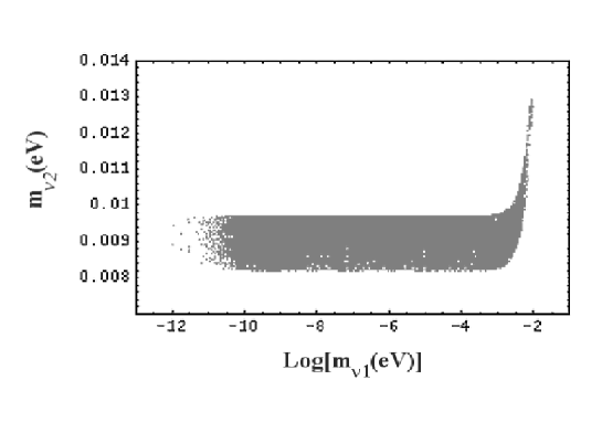
Figure 1: Predicted neutrino mass eigenvalues $m_{\nu_{1}}$ and $m_{\nu_{2}}$ (in eV).

We have found the regions of parameter space (see Section 4.4) that fit all the experimental values of lepton masses and mixings (c.f. Section 4.3). Those regions of parameter space correspond to the values of $\sin\theta_{13}$ and neutrino masses shown in Figures (1) and (2).

First, we comment Fig.(1). Except in the region where $m_{\nu_{1}}$ gets close to $10^{-2}\mbox{eV}$, $m_{\nu_{1}}$ is negligible compared to $m_{\nu_{2}}$ (so that $m_{\nu_{2}}\simeq\sqrt{\Delta m_{21}^{2}}$). The lower and upper limits on $m_{\nu_{2}}$, appearing clearly in the figure, are given, to a good approximation, by the squared roots of experimental limits on $\Delta m_{21}^{2}$ (c.f. Eq.(32)). This means that, in this large region, $m_{\nu_{2}}$ takes nearly all the possible values allowed by present experimental measurements, or in other words, that the models, and parameter space obtained here, do not yield particular predictions on $m_{\nu_{2}}$. As $m_{\nu_{1}}$ increases up to $\sim 10^{-2}\mbox{eV}$, $m_{\nu_{2}}$ also increases, thus, the difference $\Delta m_{21}^{2}$ remains well inside the allowed experimental range (32). Similarly, this region is not really predictive for $m_{\nu_{2}}$. A similar conclusion (of low predictability) also holds for $m_{\nu_{3}}$, which lies typically in the range: $[0.03,0.06]\ \mbox{eV}$, and for $m_{\nu_{1}}$, which spans several orders of magnitude as exhibits the figure.

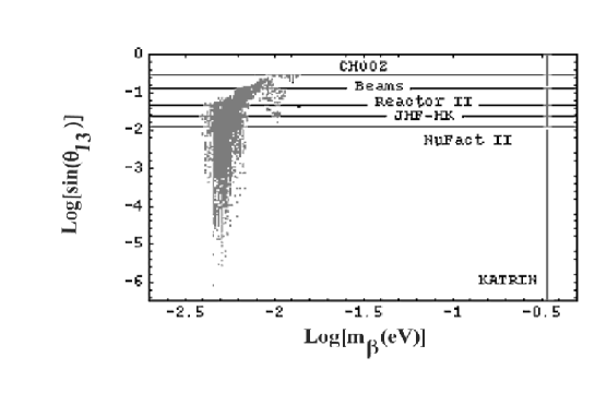
Figure 2: Predicted values for $\sin\theta_{13}$ and the effective mass $m_{\beta}$ (in eV), as defined in Section 4.3. We indicate the current CHOOZ bound on $\sin\theta_{13}$ (as issued from the three-flavor global analysis of neutrino data sample [114] mentioned in Section 4.3) as well as the best sensitivity on $\sin\theta_{13}$ expected for each type of next coming neutrino experiment (see text), namely the potential reaches for combined beam projects, JHF-HK, Reactor II and NuFact II. We also mark the maximum estimated sensitivity on $m_{\beta}$, planned to be reached by the next generation tritium beta decay experiment KATRIN, which is around $0.35\ \mbox{eV}$ [119].

In Fig.(2), we have plotted the physical quantities (predicted by our model) that will be measured by the future neutrino experiments, namely the leptonic mixing angle $\theta_{13}$ and the effective mass $m_{\beta}$ (defined in Section 4.3).
The sensitivity limits on $\sin^{2}2\theta_{13}$ at $90\%$ confidence level [110, 111] (see also [112, 113]) of future neutrino experiments, designed in particular at probing this leptonic mixing, are the following ones (for a normal neutrino mass hierarchy and best-fit values of the other oscillation parameters); for combined conventional beam experiments: $0.061$ [MINOS, plus, CNGS experiments ICARUS and OPERA], for superbeams: $0.024$ [NuMI], $0.023$ [JPARC-SK], $0.018$ [JHF-SK, a first generation long-baseline project] and $0.0021$ [JHF-HK, a second generation long-baseline beam], for reactors: $0.032$ [Double-Chooz] and $0.009$ [Reactor II, a set-up for projects like KASKA, Diablo Canyon, Braidwood,…] and for neutrino factories [109]: $0.0017$ [NuFact I, low luminosity] and $0.00059$ [NuFact II, high luminosity].
Therefore, this figure shows that the next measurements of $\sin\theta_{13}$ will only partially allow us to test the studied higher-dimensional mechanism. This is because $\sin\theta_{13}$ reaches values which are smaller than the best experimental sensitivities expected. This figure also demonstrates that future tritium beta decay experiments should not be able to test the $m_{\beta}$ values predicted by our higher-dimensional mechanism, which are too low.

So far we have only considered the normal hierarchy for the neutrino mass spectrum. An important consequence of the structure of mass matrix (21), for neutrinos, is that it is impossible to obtain degenerate, almost degenerate, or even inverse hierarchical neutrinos, unless there is some precise conspiracy between parameters $c_{i}^{L}$, $c_{j}^{\nu}$ and the Yukawa couplings $\kappa_{ij}^{\nu}$. E.g. taking $\kappa_{ij}^{\nu}=1$, clearly, leads to strict hierarchical neutrinos. The same applies if there is just one $(-)$ sign among the $\kappa_{ij}^{\nu}$ signs (see Appendix B). Two or three crucial $(-)$ signs, i.e. $(-)$ signs which cannot be eliminated by rephasing the lepton fields, may lead to 3 neutrinos with masses of the same order of magnitude, but to obtain degenerate neutrinos, one must have fine-tunning between the functions $g_{{}_{i}}(c_{i}^{L})$, $\ g^{\prime}_{{}_{j}}(c_{j}^{\nu})$ and parameters $\kappa_{ij}^{\nu}$.

6 Conclusion

The RS model, with SM fields in the bulk and the Higgs boson on the TeV-brane, has been studied. We have considered the typical values of the fundamental RS parameters ($k$, $R_{c}$ and $M_{5}$) which are compatible with all the relevant constraints: the theoretical constraints, e.g. the condition required to solve the gauge hierarchy problem, and the complete set of experimental bounds (from collider data, FC physics, precision EW measurements,…).

We have found configurations of lepton locations, along the extra dimension, reproducing all the present experimental data on leptonic masses and mixing angles, in the case where neutrinos acquire Dirac masses (with a right handed neutrino added to the SM fields). The neutrino and charged lepton sectors have been treated simultaneously since these two sectors are related phenomenologically (via the lepton mixing matrix $U_{MNS}$) and theoretically (because the left handed neutrinos and charged leptons are localized in an identical way, since they belong to the same $SU(2)_{L}$ doublet). The field location configurations, we obtained, generate the entire hierarchy among lepton masses, including the structure in flavor space, as well as, the lightness of neutrinos relatively to the charged lepton masses and electroweak scale (providing, in this sense, an alternative to the usual see-saw mechanism).

Besides, we have determined the domains of parameter space with minimum fine-tunning, in agreement with all the experimental values of leptonic masses and mixings. Then, we have deduced, from the domains, predictions on the two measurable leptonic quantities (with the exception of the physical complex phases) which are still unknown (more precisely, weakly constrained), namely the lepton mixing angle $\theta_{13}$ and the ground of neutrino mass spectrum (only the two neutrino mass squared differences are fixed by the present experimental results). We predict an approximate order of magnitude for $\sin\theta_{13}$ lying between $10^{-1}$ and $10^{-5}$. A part of this range should fall into the sensitivity interval reachable by next generation of neutrino experiments, which means that the studied mechanism, based on the localization of bulk fermions within the RS model, should be partially testable (from the parameter space point of view) by future experiments. We also predict a neutrino mass spectrum with the normal hierarchy and the smallest mass eigenvalue in the interval: $10^{-11}\mbox{eV}\lesssim m_{\nu_{1}}\lesssim 10^{-2}\mbox{eV}$. Hence, the studied model within the RS framework is not especially predictive on neutrino masses, compared e.g. to an equivalent model (also producing SM fermion mass hierarchies from flavor and nature dependent locations of fields) in the ADD framework which predicts: $m_{\nu_{1}}\sim 10^{-2}\mbox{eV}$ (for Majorana neutrino masses) [65].

Our important quantitative result is that the whole lepton mass hierarchy can be completely explained by the studied higher-dimensional mechanism, without requiring any special pattern for the Yukawa coupling constants.

Acknowledgments

The authors are grateful to G. C. Branco and M. N. Rebelo for useful conversations. G. M. acknowledges support from a Marie Curie Intra-European Fellowships (under contract MEIF-CT-2004-514138) within the 6th European Community Framework Program.

Appendix

Appendix A Fermion mass matrix

Within the studied higher-dimensional scenario where SM fermions possess various localizations along the warped extra dimension of the RS model, the effective 4-dimensional fermion Dirac mass matrix is given by,

$$M_{ij}=\ \kappa_{ij}\ m_{0}(kR_{c})\ \frac{\sqrt{1/2-c_{i}}\ \sqrt{1/2-c_{j}}}{4-c_{i}-c_{j}}\ \frac{e^{\pi kR_{c}(4-c_{i}-c_{j})}-1}{(e^{2\pi kR_{c}(1/2-c_{i})}-1)^{1/2}\ (e^{2\pi kR_{c}(1/2-c_{j})}-1)^{1/2}}.$$ (A.1)

This formula is obtained after integration of expression (11) over $y$ (on the range $[-\pi R_{c},\pi R_{c}]$), by using Eq.(8)-(9) and Eq.(12). For instance, with the value $kR_{c}=10.83$ considered in our analysis, the quantity $m_{0}(kR_{c})$ entering Eq.(A.1) reads as $m_{0}(10.83)=7.61\ 10^{-33}\mbox{eV}$.

Appendix B Sign configurations

In this appendix, we present explicit examples of $\kappa_{ij}^{l,\nu}$ sign configurations which give rise to significant lepton mixings.

$\bullet$ Let us first assume that all $\kappa_{ij}^{\nu}=\kappa_{ij}^{l}=1$ except for $\kappa_{33}^{\nu}=\kappa_{33}^{l}=-1$. Then from (21), we have

$$\begin{array}[]{ccc}\begin{array}[]{c}M_{\nu}=D_{L}\cdot\Delta^{\prime}\cdot D_{\nu}\\ \\ M_{l}=D_{L}\cdot\Delta^{\prime}\cdot D_{l}\end{array}&\ ;&\Delta^{\prime}=\left[\begin{array}[]{ccc}1&1&1\\ 1&1&1\\ 1&1&-1\end{array}\right]\end{array}$$ (B.1)

The $(-)$ sign in the $33$ position of the mass matrices $M_{\nu}$ and $M_{l}$ has two important consequences. First, it leads to a non zero mass for the muon and the second neutrino eigenstate, and secondly, it generates a large atmospheric neutrino mixing. The squared mass matrices $H_{\nu}=$ $M_{\nu}M_{\nu}^{\dagger}$ and $H_{l}=$ $M_{l}M_{l}^{\dagger}$ are now significantly different:

$$\begin{array}[]{lll}\begin{array}[]{c}H_{\nu}=\rho_{\nu}\ D_{L}\cdot\Gamma_{\nu}\cdot D_{L}\\ \\ H_{l}=\rho_{l}\ D_{L}\cdot\Gamma_{l}\cdot D_{L}\end{array}&\ ;&\Gamma_{\nu,l}=\left[\begin{array}[]{ccc}1&1&-c_{2\theta}\\ 1&1&-c_{2\theta}\\ -c_{2\theta}&-c_{2\theta}&1\end{array}\right]_{\nu,l}\end{array}$$ (B.2)

with $c_{2\theta_{\nu,l}}\equiv\cos(2\theta_{\nu,l})$ and

$$\begin{array}[]{ccc}\cos(\theta_{\nu})=\frac{b_{\nu_{3}}}{\rho_{\nu}}&\ ;&\cos(\theta_{l})=\frac{b_{l_{3}}}{\rho_{l}}\end{array}$$ (B.3)

Using a similar parameterization, as for $\rho_{\nu,l}$ in (31), for $\rho_{L}=\sqrt{a_{L1}^{2}+a_{L2}^{2}+a_{L2}^{2}}$, one finds, in this approximation, the following squared roots of eigenvalues of $H_{l}$ and $H_{\nu}$ respectively:

$$\begin{array}[]{lll}m_{e}\equiv 0&\ ;&m_{\nu_{1}}\equiv 0\\ &&\\ m_{\mu}=\frac{\rho_{L}\rho_{l}}{\sqrt{2}}\sqrt{1-\sqrt{1-s_{2\theta_{L}}^{2}s_{2\theta_{l}}^{2}}}&\ ;&m_{\nu_{2}}=\frac{\rho_{L}\rho_{\nu}}{\sqrt{2}}\sqrt{1-\sqrt{1-s_{2\theta_{L}}^{2}s_{2\theta_{\nu}}^{2}}}\\ &&\\ m_{\tau}=\frac{\rho_{L}\rho_{l}}{\sqrt{2}}\sqrt{1+\sqrt{1-s_{2\theta_{L}}^{2}s_{2\theta_{l}}^{2}}}&\ ;&m_{\nu_{3}}=\frac{\rho_{L}\rho_{\nu}}{\sqrt{2}}\sqrt{1+\sqrt{1-s_{2\theta_{L}}^{2}s_{2\theta_{\nu}}^{2}}}\end{array}$$ (B.4)

where $s_{2\theta_{\nu,l}}\equiv\sin(2\theta_{\nu,l})$ and $s_{2\theta_{L}}\equiv\sin(2\theta_{L})$, with a suitable parametrization for $(a_{1},a_{2},a_{3})_{L}$ $=$ $\rho_{L}(\sin(\varphi_{L})\sin(\theta_{L})$, $\cos(\varphi_{L})\sin(\theta_{L})$, $\cos(\theta_{L}))$. In addition, the matrices $O_{\nu,l}$ which diagonalize $H_{\nu,\,l}$ in (B.2), will have the following form

$$O_{\nu,l}=O_{\varphi_{L}}\cdot(O_{\overline{\theta}_{\nu,l}})^{T}$$ (B.5)

where

$$\begin{array}[]{ccc}O_{\varphi_{L}}=\left[\begin{array}[]{ccc}\cos(\varphi_{L})&\sin(\varphi_{L})&0\\ -\sin(\varphi_{L})&\cos(\varphi_{L})&0\\ 0&0&1\end{array}\right]&\ ;&O_{\overline{\theta}_{\nu,l}}=\left[\begin{array}[]{ccc}1&0&0\\ 0&\cos(\overline{\theta})&\sin(\overline{\theta})\\ 0&-\sin(\overline{\theta})&\cos(\overline{\theta})\end{array}\right]_{\nu,l}\end{array}$$ (B.6)

with $\tan(2\overline{\theta}_{\nu,l})=\tan(2\theta_{L})\cos(2\theta_{\nu,l})$. Notice that $O_{\varphi_{L}}$, containing the angle $\varphi_{L}$ from the parameterization of $(a_{1,}a_{2},a_{3})_{L}$, appears both in $O_{\nu}$ and $O_{l}$, and thus

$$U_{MNS}=O_{\overline{\theta}_{l}}\cdot(O_{\overline{\theta}_{\nu}})^{T}=\left[\begin{array}[]{ccc}1&0&0\\ 0&\cos(\overline{\theta})&\sin(\overline{\theta})\\ 0&-\sin(\overline{\theta})&\cos(\overline{\theta})\end{array}\right]\ ;\ \ \ \overline{\theta}=\overline{\theta}_{l}-\overline{\theta}_{\nu}$$ (B.7)

One may have large atmospheric mixing, but, unfortunately, no solar mixing. Therefore, in order to obtain sufficient large solar mixing we must have $(-)$ signs at different places in the mass matrices of the neutrinos and charged leptons.

$\bullet$ Next, we study the case $\kappa_{33}^{\nu}=\kappa_{13}^{l}=-1$ with all the other $\kappa_{ij}^{\nu}=\kappa_{ij}^{l}=1$. Due to the different position of the $(-)$ sign in the charged lepton mass matrix, we will obtain diagonalizing matrices which are significantly different. Then, it is possible to have large atmospheric and solar mixings. The permutation, induced by the different position of the $(-)$ sign, results in the following diagonalizing matrix for the charged leptons:

$$\begin{array}[]{lll}O_{l}=P\cdot O_{\widehat{\varphi}_{L}}\cdot(O_{\overline{\theta}_{l}})^{T}&\ ;&P=\left[\begin{array}[]{ccc}0&0&1\\ 0&1&0\\ 1&0&0\end{array}\right]\end{array}$$ (B.8)

where $O_{\widehat{\varphi}_{L}}$ is similar to $O_{\varphi_{L}}$, i.e. a rotation of the first and second coordinates, but where the angle $\widehat{\varphi}_{L}$ comes from a different parameterization: $(a_{1,}a_{2},a_{3})_{L}=\rho_{L}(\cos(\widehat{\theta}_{L})$, $\cos(\widehat{\varphi}_{L})\sin(\widehat{\theta}_{L})$, $\sin(\widehat{\varphi}_{L})\sin(\widehat{\theta}_{L}))$, as a result of the permutation. As in (B.6), one has $\tan(2\overline{\theta}_{l})=\tan(2\widehat{\theta}_{L})\cos(2\theta_{l})$: now related to the new $\widehat{\theta}_{L}$ of this parameterization. It is clear that, due to the permutation, $O_{\varphi_{L}}$ and $O_{\widehat{\varphi}_{L}}$ are not equal. In addition, the product $O_{\widehat{\varphi}_{L}}^{T}\cdot P\cdot O_{\varphi_{L}}$, appearing in $U_{MNS}$, does not cancel, and therefore, one may have large mixing.

References

- [1] For a review of recent developments, see K. R. Dienes, Phys. Rept. 287 (1997) 447.
- [2] T. Kaluza, Sitzungsber. Preuss. Akad. Wiss. Berlin (Math. Phys.) 1921 (1921) 966.
- [3] O. Klein, Z. Phys. 37 (1926) 895 [Surveys High Energ. Phys. 5 (1986) 241].
- [4] T. Appelquist, H.-C. Cheng and B. A. Dobrescu, Phys. Rev. D64 (2001) 035002.
- [5] K. Akama, in Gauge Theory and Gravitation, Proceedings of the International Symposium, Nara, Japan, 1982, ed. by K. Kikhawa, N. Nakanishi and H. Nariai (Springer-Verlag, 1983), 267, [arXiv:hep-th/0001113].
- [6] V. A. Rubakov and M. E. Shaposhnikov, Phys. Lett. B125 (1983) 136.
- [7] M. Visser, Phys. Lett. B159 (1985) 22.
- [8] E. J. Squires, Phys. Lett. B167 (1985) 286.
- [9] I. Antoniadis, Phys. Lett. B246 (1990) 317.
- [10] I. Antoniadis, C. Muñoz and M. Quirós, Nucl. Phys. B397 (1993) 515.
- [11] I. Antoniadis, K. Benakli and M. Quirós, Phys. Lett. B331 (1994) 313.
- [12] I. Antoniadis, S. Dimopoulos, A. Pomarol and M. Quirós, Nucl. Phys. B544 (1999) 503.
- [13] N. Arkani-Hamed, S. Dimopoulos and G. Dvali, Phys. Lett. B429 (1998) 263.
- [14] I. Antoniadis, N. Arkani-Hamed, S. Dimopoulos and G. Dvali, Phys. Lett. B436 (1998) 257.
- [15] N. Arkani-Hamed, S. Dimopoulos and G. Dvali, Phys. Rev. D59 (1999) 086004.
- [16] M. Gogberashvili, Int. J. Mod. Phys. D11 (2002) 1635, [arXiv:hep-ph/9812296].
- [17] L. Randall and R. Sundrum, Phys. Rev. Lett. 83 (1999) 3370.
- [18] I. I. Kogan, S. Mouslopoulos, A. Papazoglou, G. G. Ross and J. Santiago, Nucl. Phys. B584 (2000) 313.
- [19] S. Mouslopoulos and A. Papazoglou, JHEP 0011 (2000) 018.
- [20] I. I. Kogan, S. Mouslopoulos, A. Papazoglou and G. G. Ross, Nucl. Phys. B595 (2001) 225.
- [21] N. Kaloper, Phys. Rev. D60 (1999) 123506.
- [22] I. I. Kogan, S. Mouslopoulos and A. Papazoglou, Phys. Lett. B501 (2001) 140.
- [23] I. Oda, Phys. Lett. B480 (2000) 305.
- [24] I. Oda, Phys. Lett. B472 (2000) 59.
- [25] H. Hatanaka et al., Prog. Theor. Phys. 102 (1999) 1213.
- [26] C. Csaki and Y. Shirman, Phys. Rev. D61 (2000) 024008.
- [27] N. Arkani-Hamed, S. Dimopoulos, G. Dvali and N. Kaloper, Phys. Rev. Lett. 84 (2000) 586.
- [28] R. Gregory, V. A. Rubakov and S. M. Sibiryakov, Phys. Rev. Lett. 84 (2000) 5928.
- [29] T. Li, Phys. Lett. B478 (2000) 307.
- [30] L. Randall and R. Sundrum, Phys. Rev. Lett. 83 (1999) 4690.
- [31] J. Lykken and L. Randall, JHEP 0006 (2000) 014.
- [32] N. Kaloper, Phys. Lett. B474 (2000) 269.
- [33] S. Nam, JHEP 0003 (2000) 005.
- [34] S. Nam, JHEP 0004 (2000) 002.
- [35] For a pedagogical text, see e.g. D. Bailin and A. Love, “Supersymmetric gauge field theory and string theory”, Graduate student series in physics, Institute of physics publishing, ed. by Douglas F. Brewer.
- [36] A. Pomarol, Phys. Rev. Lett. 85 (2000) 4004.
- [37] L. Randall and M. D. Schwartz, JHEP 0111 (2001) 003.
- [38] L. Randall and M. D. Schwartz, Phys. Rev. Lett. 88 (2002) 081801.
- [39] W. D. Goldberger and I. Z. Rothstein, Phys. Rev. D68 (2003) 125011.
- [40] K. Agashe, A. Delgado and R. Sundrum, Annals Phys. 304 (2003) 145.
- [41] K. R. Dienes, E. Dudas and T. Gherghetta, Nucl. Phys. B537 (1999) 47.
- [42] Y. Nomura, D. Smith and N. Weiner, Nucl. Phys. B613 (2001) 147.
- [43] E. W. Kolb and R. Slansky, Phys. Lett. B135 (1984) 378.
- [44] G. Servant and T. M. P. Tait, Nucl. Phys. B650 (2003) 391, and references therein.
- [45] H.-C. Cheng, J. L. Feng and K. T. Matchev, Phys. Rev. Lett. 89 (2002) 211301.
- [46] D. Hooper and G. D. Kribs, Phys. Rev. D67 (2003) 055003.
- [47] K. Agashe and G. Servant, JCAP 0502 (2005) 002.
- [48] K. Agashe and G. Servant, Phys. Rev. Lett. 93 (2004) 231805.
- [49] C. D. Froggatt and H. B. Nielsen, Nucl. Phys. B147 (1979) 277.
- [50] N. Arkani-Hamed and M. Schmaltz, Phys. Rev. D61 (2000) 033005.
- [51] M. V. Libanov and S. V. Troitsky, Nucl. Phys. B599 (2001) 319; J.-M. Frère, M. V. Libanov and S. V. Troitsky, Phys. Lett. B512 (2001) 169; J.-M. Frère, M. V. Libanov and S. V. Troitsky, JHEP 0111 (2001) 025; M. V. Libanov and E. Ya. Nougaev, JHEP 0204 (2002) 055.
- [52] G. Dvali and M. Shifman, Phys. Lett. B475 (2000) 295.
- [53] P. Q. Hung, Phys. Rev. D67 (2003) 095011.
- [54] D. E. Kaplan and T. M. P. Tait, JHEP 0006 (2000) 020.
- [55] D. E. Kaplan and T. M. P. Tait, JHEP 0111 (2001) 051.
- [56] M. Kakizaki and M. Yamaguchi, Prog. Theor. Phys. 107 (2002) 433; Int. J. Mod. Phys. A19 (2004) 1715, [arXiv:hep-ph/0110266].
- [57] C. V. Chang et al., Phys. Lett. B558 (2003) 92.
- [58] S. Nussinov and R. Shrock, Phys. Lett. B526 (2002) 137.
- [59] E. A. Mirabelli and M. Schmaltz, Phys. Rev. D61 (2000) 113011.
- [60] G. Barenboim, G. C. Branco, A. de Gouvêa and M. N. Rebelo, Phys. Rev. D64 (2001) 073005.
- [61] G. C. Branco, A. de Gouvêa and M. N. Rebelo, Phys. Lett. B506 (2001) 115.
- [62] P. Q. Hung and M. Seco, Nucl. Phys. B653 (2003) 123.
- [63] H. V. Klapdor-Kleingrothaus and U. Sarkar, Phys. Lett. B541 (2002) 332.
- [64] M. Raidal and A. Strumia, Phys. Lett. B553 (2003) 72.
- [65] J.-M. Frère, G. Moreau and E. Nezri, Phys. Rev. D69 (2004) 033003.
- [66] T. Gherghetta and A. Pomarol, Nucl. Phys. B586 (2000) 141.
- [67] D. Dooling and K. Kang, Phys. Lett. B502 (2001) 189.
- [68] K. R. Dienes, E. Dudas and T. Gherghetta, Phys. Lett. B436 (1998) 55.
- [69] K. R. Dienes, E. Dudas and T. Gherghetta, Nucl. Phys. B537 (1999) 47.
- [70] K. Yoshioka, Mod. Phys. Lett. A15 (2000) 29.
- [71] M. Bando, T. Kobayashi, T. Noguchi and K. Yoshioka, Phys. Rev. D63 (2001) 113017.
- [72] A. Neronov, Phys. Rev. D65 (2002) 044004.
- [73] N. Arkani-Hamed et al., Phys. Rev. D61 (2000) 116003.
- [74] K. R. Dienes, E. Dudas and T. Gherghetta, Nucl. Phys. B557 (1999) 25.
- [75] N. Arkani-Hamed et al., Phys. Rev. D65 (2002) 024032.
- [76] N. Arkani-Hamed and S. Dimopoulos, Phys. Rev. D65 (2002) 052003, [arXiv:hep-ph/9811353].
- [77] Y. Grossman and M. Neubert, Phys. Lett. B474 (2000) 361.
- [78] T. Appelquist et al., Phys. Rev. D65 (2002) 105019.
- [79] T. Gherghetta, Phys. Rev. Lett. 92 (2004) 161601.
- [80] G. Moreau, Eur. Phys. J. C40 (2005) 539.
- [81] S. J. Huber and Q. Shafi, Phys. Lett. B498 (2001) 256.
- [82] S. J. Huber and Q. Shafi, Phys. Lett. B544 (2002) 295.
- [83] S. J. Huber and Q. Shafi, Phys. Lett. B583 (2004) 293.
- [84] S. J. Huber and Q. Shafi, Phys. Lett. B512 (2001) 365.
- [85] H. Davoudiasl, J. L. Hewett and T. G. Rizzo, Phys. Lett. B473 (2000) 43.
- [86] A. Pomarol, Phys. Lett. B486 (2000) 153.
- [87] S. Chang et al., Phys. Rev. D62 (2000) 084025.
- [88] B. Bajc and G. Gabadadze, Phys. Lett. B474 (2000) 282.
- [89] R. Jackiw and C. Rebbi, Phys. Rev. D13 (1976) 3398.
- [90] A. Kehagias and K. Tamvakis, Phys. Lett. B504 (2001) 38.
- [91] W. D. Goldberger and M. B. Wise, Phys. Rev. Lett. 83 (1999) 4922.
- [92] S. J. Huber, Nucl. Phys. B666 (2003) 269.
- [93] J. L. Hewett, F. J. Petriello and T. G. Rizzo, JHEP 0209 (2002) 030.
- [94] C. S. Kim, J. D. Kim and J. Song, Phys. Rev. D67 (2003) 015001.
- [95] S. J. Huber and Q. Shafi, Phys. Rev. D63 (2001) 045010.
- [96] S. J. Huber, C.-A. Lee and Q. Shafi, Phys. Lett. B531 (2002) 112.
- [97] H. Davoudiasl, J. L. Hewett and T. G. Rizzo, Phys. Rev. D63 (2001) 075004.
- [98] G. Burdman, Phys. Rev. D66 (2002) 076003.
- [99] F. del Aguila and J. Santiago, Phys. Lett. B493 (2000) 175.
- [100] H. Davoudiasl, J. L. Hewett and T. G. Rizzo, Phys. Lett. B493 (2000) 135.
- [101] K. Agashe et al., JHEP 0308 (2003) 050.
- [102] F. del Aguila, M. Perez-Victoria and J. Santiago, JHEP 0302 (2003) 051.
- [103] M. Carena, T. M. P. Tait and C. E. M. Wagner, Acta Phys. Polon. B33 (2002) 2355.
- [104] M. Carena, E. Ponton, T. M. P. Tait and C. E. M. Wagner, Phys. Rev. D67 (2003) 096006.
- [105] M. Carena et al., Phys. Rev. D68 (2003) 035010.
- [106] M. Carena et al., Phys. Rev. D71 (2005) 015010.
- [107] A. Pompos (On behalf of the CDF and the D0 Collaborations), Proceedings of the Workshop on Deep Inelastic Scattering 2004 (DIS 2004), Strbske Pleso, Slovakia, June 14-18, 2004, [arXiv:hep-ex/0408004].
- [108] M. K. Unel, Proceedings, Hadron Collider Physics (HCP 2004), Michigan, USA, E. Lansing, [arXiv:hep-ex/0411067].
- [109] M. Apollonio et al. (CERN working group on oscillation physics at the Neutrino Factory), CERN Yellow Report on the Neutrino Factory, [arXiv:hep-ph/0210192].
- [110] P. Huber, M. Lindner and W. Winter, Nucl. Phys. B645 (2002) 3.
- [111] P. Huber et al., Phys. Rev. D70 (2004) 073014.
- [112] P. Huber et al., Nucl. Phys. B665 (2003) 487.
- [113] K. Cheung, Plenary talk given at the 12th International Conference on Supersymmetry and Unification of Fundamental Interactions (SUSY 2004), Tsukuba, Japan, June 17-23, 2004, [arXiv:hep-ph/0409028].
- [114] M. Maltoni, T. Schwetz, M. A. Tortola, J. W. F. Valle, New J. Phys. 6 (2004) 122, [arXiv:hep-ph/0405172].
- [115] Particle Data Group, K. Hagiwara et al., Phys. Rev. D66 (2002) 010001.
- [116] Y. Farzan, O. L. G. Peres and A. Yu. Smirnov, Nucl. Phys. B612 (2001) 59.
- [117] J. Bonn et al., Nucl. Phys. Proc. Suppl. 91 (2001) 273.
- [118] V. M. Lobashev et al., Phys. Lett. B460 (1999) 227; Nucl. Phys. Proc. Suppl. 77 (1999) 327; 91 (2001) 280.
- [119] A. Osipowicz et al. [KATRIN Collaboration], [arXiv:hep-ex/0109033].
- [120] J. I. Silva-Marcos, JHEP0307 (2003) 012; G. C. Branco, M. N. Rebelo and J. I. Silva-Marcos, Nucl. Phys. B686 (2204) 188.