TUM–HEP–596/05
hep–ph/0507143 Deviations from Tribimaximal Neutrino Mixing

Abstract

Current neutrino data are consistent with the so–called tribimaximal mixing scenario, which predicts $\sin^{2}\theta_{12}=1/3$, zero $U_{e3}$ and maximal $\theta_{23}$. This implies a special form of the neutrino mass matrix. Introducing small breaking terms in this mass matrix generates deviations from the tribimaximal scheme and leads to testable correlations between the parameters. They depend on where the perturbation is located in the mass matrix. A special case of such perturbations are radiative corrections. Alternative deviations from tribimaximal mixing may stem from contributions of the charged lepton sector. If there is quark–lepton–unification and it is the CKM matrix which corrects the tribimaximal mixing scheme, then almost maximal $CP$ violation and sizable deviation from zero $U_{e3}$ are implied.

1 Introduction

Neutrino physics aims to fully determine all parameters of the neutrino mass matrix [1]. Six out of the 9 physical low energy parameters are contained in the Pontecorvo–Maki–Nakagawa–Sakata (PMNS) neutrino mixing matrix [2]. It is given in general by $U=U_{\ell}^{\dagger}\,U_{\nu}$, where $U_{\nu}$ diagonalizes the neutrino mass matrix and $U_{\ell}$ is associated to the diagonalization of the charged lepton mass matrix. The PMNS matrix can be parametrized as

$$\begin{array}[]{c}U=\left(\begin{array}[]{ccc}c_{12}c_{13}&s_{12}c_{13}&s_{13}e^{-i\delta}\\[5.69046pt] -s_{12}c_{23}-c_{12}s_{23}s_{13}e^{i\delta}&c_{12}c_{23}-s_{12}s_{23}s_{13}e^{i\delta}&s_{23}c_{13}\\[5.69046pt] s_{12}s_{23}-c_{12}c_{23}s_{13}e^{i\delta}&-c_{12}s_{23}-s_{12}c_{23}s_{13}e^{i\delta}&c_{23}c_{13}\\ \end{array}\right){\rm diag}(1,e^{i\alpha},e^{i(\beta+\delta)})\,,\end{array}$$ (1)

where we have used the usual notations $c_{ij}=\cos\theta_{ij}$, $s_{ij}=\sin\theta_{ij}$, $\delta$ is the Dirac $CP$ violation phase, $\alpha$ and $\beta$ are two possible Majorana $CP$ violation phases [3]. The values of the currently known mixing parameters are at $3\sigma$ [4, 5]:

$$\sin^{2}\theta_{12} = 0.24\ldots 0.41\;,$$

$$|U_{e3}|^{2} \leq 0.044\;,$$ (2)

$$\sin^{2}\theta_{23} = 0.34\ldots 0.68\;.$$

The probably most puzzling aspect of those numbers is that two of the mixing angles are compatible with two extreme values, namely zero for $\theta_{13}$ and $\pi/4$ for $\theta_{23}$. If confirmed by future data, this will be a strong hint towards the presence of special non–trivial symmetries in the lepton sector.

Regarding the neutrino masses, we neither do know what the precise value of the lightest mass state is, nor do we know whether neutrinos are normally or inversely ordered. Instead, we have some information on the mass squared differences whose ratio is, again at $3\sigma$, given by [4]

$$R\equiv\frac{\Delta m^{2}_{\odot}}{\Delta m^{2}_{\rm A}}=\frac{m_{2}^{2}-m_{1}^{2}}{\left|m_{3}^{2}-m_{1}^{2}\right|}=\frac{(7.1\ldots 8.9)\cdot 10^{-5}}{(1.4\ldots 3.3)\cdot 10^{-3}}=0.0215\ldots 0.0636\;.$$ (3)

Many models have been constructed [6] in order to explain the mass and mixing schemes as implied by the data. A particularly interesting mixing scenario, which is compatible with all current data, is the so–called tribimaximal scenario [7, 8, 9, 10], defined by the following PMNS matrix:

$$U=\left(\begin{array}[]{ccc}\sqrt{\frac{2}{3}}&\sqrt{\frac{1}{3}}&0\\[5.69046pt] -\sqrt{\frac{1}{6}}&\sqrt{\frac{1}{3}}&\sqrt{\frac{1}{2}}\\[5.69046pt] \sqrt{\frac{1}{6}}&-\sqrt{\frac{1}{3}}&\sqrt{\frac{1}{2}}\end{array}\right)~{}.$$ (4)

It corresponds to $\sin^{2}\theta_{12}=1/3$, $U_{e3}=0$ and $\theta_{23}=\pi/4$. These numbers are referred to as “tribimaximal values” in this paper. Many authors have considered this scenario from various points of view [7, 8, 9, 10]. We would like to note here that the most recent SNO salt phase data [12] shifted the central value of $\sin^{2}\theta_{12}$ to slightly higher values (the best–fit point went from 0.29 to 0.31 [5]). In addition, the allowed range of $\sin^{2}\theta_{12}$ is now centered around the value 1/3 more than before (from $0.21\ldots 0.38$ or $1/3\,^{+0.05}_{-0.12}$ to $0.24\ldots 0.41$ or $1/3\,^{+0.08}_{-0.09}$). Hence, tribimaximal mixing is more than ever an interesting mixing scheme to investigate.

In the future one expects some improvement on our knowledge of the neutrino mixing parameters (for summaries and more references, see for instance [13]). For our purposes, we mention that (at 3$\sigma$) next generation reactor and long–baseline experiments will probe $U_{e3}$ ($\sin^{2}\theta_{23}-1/2$) down to the 5 $\%$ (10 $\%$) level [14]. Further precision requires far–future projects such as neutrino factories or beta–beams. Low energy solar neutrino experiments [15] can probe $\sin^{2}\theta_{12}$ with an uncertainty of $\sim 15\%$, whereas more precision could stem from reactor experiments with a baseline corresponding to an oscillation minimum [16].

In this letter we wish to analyze the predictions of two different methods to perturb the tribimaximal mixing scenario. Instead of constructing models which realize such corrections, we rather give a summary of many possible scenarios. This will hopefully give a feeling for the expected values (in particular) of $\theta_{12,13,23}$ which can follow from models leading to (approximate) tribimaximal mixing. First, we assume in Section 2 that the symmetry basis coincides with the basis in which the charged lepton mass matrix is real and diagonal. We then introduce at different positions in the mass matrix small breaking parameters and analyze the resulting predictions for the oscillation parameters.

The second approach lies in the impact of contributions from the charged lepton sector via $U_{\ell}$ to $U_{\nu}$. The latter matrix is assumed to correspond to tribimaximal mixing. This is discussed in Section 3. We present our conclusions and final remarks in Section 4.

2 Perturbing the Mass Matrix

We shall work in this Section in a basis in which the charged leptons are real and diagonal, i.e., $U_{\ell}=\mathbbm{1}$. In general, a neutrino mass matrix leading to the predictions $\sin^{2}\theta_{12}=1/3$, $U_{e3}=0$ and $\theta_{23}=\pi/4$ has the form

$$m_{\nu}=\left(\begin{array}[]{ccc}A&B&-B\\[5.69046pt] \cdot&\frac{1}{2}(A+B+D)&\frac{1}{2}(D-A-B)\\[5.69046pt] \cdot&\cdot&\frac{1}{2}(A+B+D)\end{array}\right)~{},$$ (5)

where

$$A=\frac{1}{3}(2\,m_{1}+e^{i\alpha}\,m_{2})~{},~{}~{}B=\frac{1}{3}(e^{i\alpha}\,m_{2}-m_{1})~{},~{}~{}D=e^{i\beta}\,m_{3}~{},$$ (6)

or $m_{1}=A-B$ and $e^{i\alpha}\,m_{2}=A+2\,B$. Interestingly, removing $B$ from the $\mu$–$\tau$ block of Eq. (5) will give $\sin^{2}\theta_{12}=1/2$, i.e., exactly bimaximal mixing [17]. As well known, both the tribimaximal and the bimaximal mixing scheme are special cases of $\mu$–$\tau$ symmetric matrices, whose generic predictions are $U_{e3}=0$ and $\theta_{23}=\pi/4$ [18, 19, 20].

Depending on the neutrino mass spectrum, the above neutrino mass matrix Eq. (5) simplifies further:

• in case of an extreme normal hierarchy (NH) we have $m_{1}\simeq 0$ and consequently $A\simeq B$ with $|A|,|B|\ll|D|$;

• in case of an extreme inverted hierarchy (IH) we have $m_{3}=D\simeq 0$. If in addition $m_{2}$ and $m_{1}$ have opposite (identical) $CP$ parities, one has $A\simeq\sqrt{\mbox{$\Delta m^{2}_{\rm A}$}}/3$ and $B\simeq-2\sqrt{\mbox{$\Delta m^{2}_{\rm A}$}}/3$ ($A\simeq\sqrt{\mbox{$\Delta m^{2}_{\rm A}$}}$ and $B\simeq 0$);

• in case of a quasi–degenerate spectrum we can neglect the mass splittings and have for equal $CP$ parities of $m_{1}$ and $m_{2}$ that $B\simeq 0$ and $|A|\simeq|D|$. If in addition $m_{3}$ has the same parity as $m_{1}$ and $m_{2}$, then the mass matrix is proportional to the unit matrix: $m_{\nu}=A\,\mathbbm{1}\simeq m_{0}\,\mathbbm{1}$. If $m_{1}$ and $m_{2}$ have opposite parities, then $A\simeq m_{0}/3\simeq-B/2$ and $|A|\simeq|D|/3$. If sgn($m_{1}$)= sgn($m_{2}$)=$-$sgn($m_{3}$), then $A\simeq-D$, $B=0$ and all elements of the mass matrix are zero except for the $ee$ entry $A$, and the $\mu\tau$ entry $-A$. This matrix conserves the flavor charge $L_{\mu}-L_{\tau}$ [21] and has for instance been obtained also in Refs. [22].

In this letter we shall focus on the normal and inverted hierarchical case, since radiative corrections, in particular for $\theta_{12}$, are in general very strong for quasi–degenerate neutrinos.

In the following Subsections we shall analyze perturbations of the tribimaximal mass matrix. With perturbations we mean that an element of the matrix Eq. (5) is multiplied with $(1+\epsilon)$, where $\epsilon\ll 1$. These corrections might stem for instance from higher dimensional Higgs representations of the underlying theory which generates tribimaximal mixing or by the fact that the theory does not exactly reproduce the matrix in Eq. (5). There are two cases which result in deviations of all three mixing parameters, namely perturbations in the $e\tau$ element or in the $\mu\mu$ element. They are equivalent to perturbations in the $e\mu$ element or in the $\tau\tau$ element when the sign of $\epsilon$ is changed. Alternatively, one can perturb the $ee$ or $\mu\tau$ element of $m_{\nu}$ and one will find that only the relation $\sin^{2}\theta_{12}=1/3$ is altered, whereas $U_{e3}=0$ and $\theta_{23}=\pi/4$ remain. This is because the $\mu$–$\tau$ symmetry is unchanged when the $ee$ or $\mu\tau$ element are altered. In Section 2.1 and 2.2 we analyze these possibilities in case of NH and IH, respectively. The case of applying radiative corrections to the mass matrix is treated separately in Section 2.3.

2.1 Normal Hierarchy

Let us consider first the case of normal hierarchy, i.e., $|D|\gg|A|,|B|$. It is known from the study of $\mu$–$\tau$ symmetric matrices that if the symmetry is broken in the electron sector, $|U_{e3}|$ deviates more from zero than $\theta_{23}$ does from $\pi/4$ [23]. Indeed, the matrix which is obtained by perturbing the $e\tau$ element,

$$m_{\nu}^{\prime}=\left(\begin{array}[]{ccc}A&B&-B(1+\epsilon)\\[5.69046pt] \cdot&\frac{1}{2}(A+B+D)&\frac{1}{2}(D-A-B)\\[5.69046pt] \cdot&\cdot&\frac{1}{2}(A+B+D)\end{array}\right)~{},$$ (7)

predicts that $\theta_{23}$ remains rather close to maximal, $\theta_{23}=\pi/4+{\cal O}(\epsilon^{2})$, and

$$\sin^{2}\theta_{12}\simeq\frac{1}{3}\left(1+\frac{2}{9}\,\epsilon\right)~{}\mbox{ and }~{}|U_{e3}|\simeq\frac{\epsilon}{\sqrt{2}}\frac{B}{D}\simeq\frac{m_{2}-m_{1}}{3\sqrt{2}\,m_{3}}\,\epsilon\simeq\frac{\sqrt{R}}{3\,\sqrt{2}}\,\epsilon~{}.$$ (8)

Note that the parameters $A,B,D$ drop out of the expression for $\sin^{2}\theta_{12}$, leading to a sharp prediction for solar neutrino mixing as a function of $\epsilon$. The parameter $|U_{e3}|$ is suppressed by the small breaking parameter $\epsilon$ and by the ratio $(m_{2}-m_{1})/m_{3}$, which is roughly the square root of the solar and atmospheric $\Delta m^{2}$. In total, one therefore expects that $|U_{e3}|\mathrel{\hbox to0.0pt{\raise 2.20013pt\hbox{$<$}\hss}{\lower 2.20013pt\hbox{$\sim$}}}R$. We can write down the following correlations between the observables:

$$\sin^{2}\theta_{12}\simeq\frac{1}{3}\left(1+\frac{2\sqrt{2}}{3}\,\frac{|U_{e3}|}{\sqrt{R}}\right)~{}\mbox{ and }~{}\mbox{$\langle m\rangle$}\simeq\frac{\sqrt{\mbox{$\Delta m^{2}_{\odot}$}}}{3}\simeq\frac{2\sqrt{2}}{27}\frac{|U_{e3}|\,\sqrt{\mbox{$\Delta m^{2}_{\rm A}$}}}{\sin^{2}\theta_{12}-\frac{1}{3}}~{}.$$ (9)

The last equation holds in the limit $A\simeq B$, which corresponds to a very strong hierarchy of the neutrino masses. Of course, the effective mass in case of NH is very small.

Now we perturb the tribimaximal mixing scenario in the $\mu\mu$ element, such that

$$m_{\nu}^{\prime}=\left(\begin{array}[]{ccc}A&B&-B\\[5.69046pt] \cdot&\frac{1}{2}(A+B+D)(1+\epsilon)&\frac{1}{2}(D-A-B)\\[5.69046pt] \cdot&\cdot&\frac{1}{2}(A+B+D)\end{array}\right)~{}.$$ (10)

Then it holds for $A\simeq B$ that

$$\sin^{2}\theta_{23}\simeq\frac{1}{2}\left(1+\frac{\epsilon}{2}\right)~{},~{}|U_{e3}|\simeq\frac{\epsilon}{2\sqrt{2}}\,\frac{B}{D}~{}.$$ (11)

In contrast to the case of breaking in the $e$ sector, we have in the expressions for the mass eigenstates now terms of order $B$ and $D\epsilon$, which might be all of the same order. This prohibits to directly connect $B/D$ with the ratio of the mass–squared differences. Nevertheless, $B/D$ is of the order of $\sqrt{R}$, so that a similar magnitude for $|U_{e3}|$ as in case of a perturbation in the $e\tau$ element is expected. For the solar neutrino mixing angle we find

$$\tan 2\theta_{12}\simeq\frac{2\sqrt{2}}{1+D/B\,\epsilon/4}~{},$$ (12)

where in contrast to the previous case the parameters $B$ and $D$, which are connected to the masses, appear. Thus, as a function of $\epsilon$ there will now be a sizable spread in the allowed values of $\sin^{2}\theta_{12}$. We can rewrite the last formulae as

$$\tan 2\theta_{12}\simeq\frac{2\sqrt{2}}{1+(\sin^{2}\theta_{23}-1/2)^{2}/(8\sqrt{2}\,|U_{e3}|)}\simeq\frac{2\sqrt{2}}{1+(\sin^{2}\theta_{23}-1/2)\,\sqrt{\mbox{$\Delta m^{2}_{\rm A}$}}/\mbox{$\langle m\rangle$}}~{},$$ (13)

where the last estimate is valid for $A\simeq B$. From the approximative expressions for the mixing parameters, we expect that both the deviations of $\sin^{2}\theta_{12}$ from $1/3$ and of $\sin^{2}\theta_{23}$ from $1/2$ are larger when breaking occurs in the $\mu\mu$ element.

We relax now the assumption of an extreme hierarchy $A\simeq B\ll D$ and consider the case that $|A|$ and $|B|$ are of the same order and one order of magnitude smaller than $|D|$. Allowing further that those quantities are complex, we turn to a numerical analysis. Fig. 2 shows the results, which confirm our analytical estimates from above. In order to generate this plot we required the oscillation parameters to lie in their allowed 3$\sigma$ ranges given in Eqs. (1, 3) and used the mass matrices from Eqs. (7, 10) with a fixed value of $\epsilon=0.1$. As can be seen from the approximate expressions in Eqs. (8, 11, 12), the direction in which the deviations of $\sin^{2}\theta_{12}$ and $\sin^{2}\theta_{23}$ from their tribimaximal values go depend on the sign of $\epsilon$. This change of sign is equivalent to a relocation of the perturbation. For instance, for positive $\epsilon$ and a perturbation in the $e\tau$ element, we have $\sin^{2}\theta_{12}>1/3$. If $\epsilon$ is negative or we break the symmetry in the $e\mu$ element with positive $\epsilon$, we would have $\sin^{2}\theta_{12}<1/3$.

Other breaking scenarios may be possible, for instance, one might perturb only the $ee$ element of Eq. (5). Then $U_{e3}$ and $\theta_{23}$ will keep their values 0 and $\pi/4$, respectively, and only the solar neutrino mixing angle will be modified, according to

$$\sin^{2}\theta_{12}\simeq\frac{1}{3}\left(1+\frac{4}{9}\frac{A}{B}\,\epsilon\right)~{},$$ (14)

where $A/B$ is approximately equal to one for NH. The deviation is therefore small. Perturbing the $\mu\tau$ entry of $m_{\nu}$ also leaves $U_{e3}$ and $\theta_{23}$ unchanged and leads to

$$\sin^{2}\theta_{12}\simeq\frac{1}{3}\left(1-\frac{2}{9}\frac{A+B-D}{B}\,\epsilon\right)~{}.$$ (15)

The deviation from 1/3 is rather sizable, since $(A+B-D)/B\sim 1/\sqrt{R}$. Hence, $\sin^{2}\theta_{12}$ lies typically close to its maximal allowed value.

2.2 Inverted Hierarchy

Now we turn to the inverted hierarchy, where the requirement of stability under renormalization motivates us to study the case $A\simeq-B/2$. This can be understood from Eq. (6) which states that for $A\simeq-B/2$ the two leading mass states possess opposite $CP$ parity. This stabilizes the oscillation parameters connected to solar neutrinos [24]. For effects solely attributed to radiative corrections, see Section 2.3. First we consider breaking in the $e\tau$ entry of Eq. (5), i.e., the matrix from Eq. (7). Setting $D=0$ we have

$$\sin^{2}\theta_{12}\simeq\frac{1}{3}\left(1+\frac{2}{9}\,\epsilon\right)~{},~{}|U_{e3}|\simeq\frac{A+B}{2\sqrt{2}\,B}\,\epsilon\simeq\frac{1}{4\sqrt{2}}\,\epsilon\simeq\sqrt{\frac{3}{14}}\,\sqrt{R}~{},$$ (16)

where the last estimates for $|U_{e3}|$ are valid for $A\simeq-B/2$. In this case we also have $\sin^{2}\theta_{12}\simeq 1/3~{}(1+8\sqrt{2}\,\epsilon/9)$. In contrast to the case of normal hierarchy given above, atmospheric neutrino mixing can deviate significantly from maximal, namely

$$\sin^{2}\theta_{23}\simeq\frac{1}{2}(1+\epsilon)\simeq\frac{1}{2}\left(1+4\sqrt{2}\,|U_{e3}|\right)~{}.$$ (17)

The parameters $A,B,D$ drop out of the expressions for $\sin^{2}\theta_{12}$ and $\sin^{2}\theta_{23}$, leading to a sharp prediction for this observable.

The next case is to break the symmetry in the $\mu\mu$ element, i.e., we consider Eq. (10) with $D\ll A\simeq-B/2$. As a result,

$$|U_{e3}|\simeq\frac{A+B}{4\sqrt{2}\,B}\,\epsilon\simeq\frac{1}{8\sqrt{2}}\,\epsilon~{},~{}\sin^{2}\theta_{23}\simeq\frac{1}{2}\left(1-\frac{A(A+B)}{2\sqrt{2}\,B}\,\epsilon\right)\simeq\frac{1}{2}\left(1-\frac{1}{8\sqrt{2}}\,\epsilon\right)~{},$$ (18)

which shows that $U_{e3}$ and $\sin^{2}\theta_{23}$ witness only small corrections. What regards the solar neutrino mixing parameter,

$$\sin^{2}\theta_{12}\simeq\frac{1}{3}\left(1-\frac{A+B}{9\,B}\,\epsilon\right)\simeq\frac{1}{3}\left(1-\frac{1}{18}\,\epsilon\right)~{}.$$ (19)

As already noted in [23], the correlation between $|U_{e3}|$ and $R$ is not particularly strong or even absent in case of IH. The estimates for the solar neutrino parameters are not very reliable in this case. Again, we present a numerical analysis of the general consequences. We assume that $|D|$ is one order of magnitude smaller than $|A|,|B|$, which in turn fulfill $|A|\simeq-|B|/2$. Diagonalizing with such values the matrices from (7, 10) gives Fig. 2 (again for $\epsilon=0.1$), which confirms our analytical estimates. We also display the ratio $\mbox{$\Delta m^{2}_{\rm A}$}/\mbox{$\langle m\rangle$}$ in this Figure. Note that with opposite parities of the two mass states in case of IH it holds that $\mbox{$\langle m\rangle$}\simeq\sqrt{\mbox{$\Delta m^{2}_{\rm A}$}}\,\cos 2\theta_{12}$, where for exact tribimaximal mixing $\cos 2\theta_{12}=\sin^{2}\theta_{12}=1/3$. Again, changing the sign of $\epsilon$ (or perturbing the matrix in the $e\mu$ ($\tau\tau$) instead of the $e\tau$ ($\mu\mu$) element) leads approximately to a reflection of $\sin^{2}\theta_{12}$ and $\sin^{2}\theta_{23}=1/2$ around their tribimaximal values.

One can again perturb the $ee$ or the $\mu\tau$ element, which does not change $U_{e3}=0$ or $\sin^{2}\theta_{23}=1/2$ but alters $\theta_{12}$ according to Eqs. (14, 15). In our case of opposite $CP$ parities we have for a perturbation in the $ee$ element that $\sin^{2}\theta_{12}\simeq\frac{1}{3}+\frac{4}{27}\frac{A}{B}\,\epsilon$ with $A/B\simeq-1/2$. Perturbing the $\mu\tau$ element also gives negligible corrections, namely $\sin^{2}\theta_{12}\simeq\frac{1}{3}-\epsilon/27$.

2.3 Radiative Corrections

Radiative corrections [24] can also play a role to generate deviations from tribimaximal mixing. Running from a high scale $M_{X}\simeq 10^{16}$ GeV at which the tribimaximal mass matrix is assumed to be generated to the low scale has an effect on the mass matrix Eq. (5) of

$$m_{\nu}^{\prime}=\left(\begin{array}[]{ccc}A&B&-B(1+\epsilon)\\[5.69046pt] \cdot&\frac{1}{2}\left(A+B+D\right)&\frac{1}{2}(D-A-B)(1+\epsilon)\\[5.69046pt] \cdot&\cdot&\frac{1}{2}(A+B+D)(1+2\epsilon)\end{array}\right),\mbox{where }\epsilon=c\,\frac{m_{\tau}^{2}}{16\pi^{2}\,v^{2}}\ln\frac{M_{X}}{m_{Z}}~{}.$$ (20)

The parameter $c$ is given by 3/2 in the SM and by $-(1+\tan^{2}\beta)$ in the MSSM. We find that in the SM there are no sizable effects on the observables. In case of the MSSM, however, interesting effects occur for NH and $\tan\beta\mathrel{\hbox to0.0pt{\raise 2.20013pt\hbox{$>$}\hss}{\lower 2.20013pt\hbox{$\sim$}}}30$. We calculate in case of a normal hierarchy the observables to be

$$|U_{e3}|\simeq\frac{\sqrt{2}B}{D}\epsilon~{},~{}~{}\sin^{2}\theta_{23}\simeq\frac{1}{2}(1-\epsilon)~{}\mbox{ and }~{}\sin^{2}\theta_{12}\simeq\frac{1}{3}\left(1-\frac{2}{9}(1+2\,A/B)\,\epsilon\right)~{}.$$ (21)

With negative $\epsilon$, as in the case of the relevant corrections in the MSSM, we have $\sin^{2}\theta_{23}$ above $1/2$ and $\sin^{2}\theta_{23}$ above $1/3$.

Considering IH we have two cases, corresponding to $|A|\simeq|B|/2\gg|D|$ and $|A|\gg|B|,|D|$. The first possibility implies opposite $CP$ parities of the leading mass states and the second one identical parities, which is known to be unstable under radiative corrections [24]. It turns out that in this case there is indeed an upper limit on $\tan\beta$, given by roughly $\tan\beta\mathrel{\hbox to0.0pt{\raise 2.20013pt\hbox{$>$}\hss}{\lower 2.20013pt\hbox{$\sim$}}}15$, i.e., larger values are not compatible with the data. Both cases imply that $U_{e3}$ is small, namely of order $\epsilon^{2}$ or $\epsilon\,D/A$. For $|A|\simeq|B|/2\gg|D|$ we find that

$$\sin^{2}\theta_{12}\simeq\frac{1}{3}\left(1-\frac{2}{9\,B}(2A+B)\,\epsilon\right)~{}\mbox{ and }~{}\sin^{2}\theta_{23}\simeq\frac{1}{2}\left(1+\epsilon\right)~{}.$$ (22)

Therefore, with negative $\epsilon$ we have $\sin^{2}\theta_{12}>1/3$ and $\sin^{2}\theta_{12}<1/2$. The same is implied for the rather unstable case of $|A|\gg|B|,|D|$, for which we find

$$\tan 2\theta_{12}\simeq\frac{2\sqrt{2}~{}(1+\epsilon)}{1+(1+A/B\,\epsilon)}~{}\mbox{ and }~{}\sin^{2}\theta_{23}\simeq\frac{1}{2}(1+\epsilon)~{}.$$ (23)

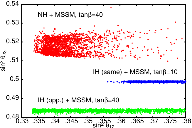
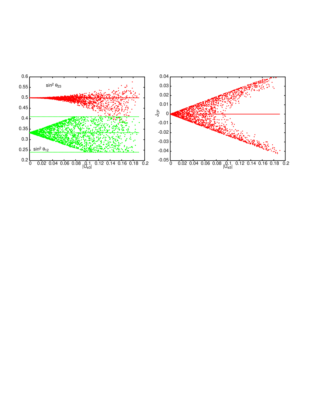
Figure 3: Scatter plot of $\sin^{2}\theta_{12}$ against $\sin^{2}\theta_{23}$ generated by radiative corrections for different situations resulting from Eq. (20). The parameters $A,B,D$ are taken complex. “NH” means that $|D|\gg|A|,|B|$, “IH (opp.)” $|A|\simeq|B|/2\gg|D|$ and “IH (same)” $|A|\gg|B|,|D|$.

Figure 4: Scatter plot of $|U_{e3}|$ against $\sin^{2}\theta_{12}$ and $\sin^{2}\theta_{23}$ and against $J_{CP}$ for a “CKM–like” matrix $U_{\ell}$. Note that the ranges of $\sin^{2}\theta_{12}$ and $\sin^{2}\theta_{23}$ can overlap.

As expected, $\theta_{12}$ receives sizable corrections, since $A/B\sim 1/\sqrt{R}$. Interestingly, $\sin^{2}\theta_{12}$ is always larger than 1/3 when radiative corrections are applied. We plot in Fig. 4 some of the resulting scatter plots. The parameter $U_{e3}$ is below 0.01 in all three cases.

3 Perturbing the Mixing Matrix

The second possibility to deviate a zeroth order mixing scheme is by taking correlations from the charged lepton sector into account. This approach has been followed mainly to analyze deviations from bimaximal neutrino mixing [25, 26, 27], but also has been studied in case of deviations from tribimaximal mixing [9, 10], where similar studies can be found. We note here that the analysis in this Section is independent on the mass hierarchy of the neutrinos. In general, the PMNS matrix is given by

$$U=U^{\dagger}_{\ell}\,U_{\nu}~{},$$ (24)

where $U_{\ell}$ is the $3\times 3$ unitary matrix associated with the diagonalization of the charged lepton mass matrix and $U_{\nu}$ diagonalizes the neutrino Majorana mass term. As has been shown in Ref. [27], one can in general express the PMNS matrix as

$$U=\tilde{U}_{\ell}^{\dagger}\,P_{\nu}\,\tilde{U}_{\nu}\,Q_{\nu}~{}.$$ (25)

It consists of two diagonal phase matrices $P_{\nu}$ = diag($1,e^{i\phi},e^{i\omega}$) and $Q_{\nu}$ = diag($1,e^{i\rho},e^{i\sigma}$), as well as two “CKM–like” matrices $\tilde{U}_{\ell}$ and $\tilde{U}_{\nu}$ which contain three mixing angles and one phase each, and are parametrized in analogy to Eq. (1). All matrices except for $\tilde{U}_{\ell}$ stem from the neutrino sector and out of the six phases present in Eq. (25) five stem from the neutrino sector. We denote the phase in $\tilde{U}_{\ell}$ with $\psi$. The six phases will in general contribute in a complicated manner to the three observable ones. In case of one angle in $U_{\nu}$ being zero, the phase in $\tilde{U}_{\nu}$ is unphysical. Note that the 2 phases in $Q_{\nu}$ do not appear in observables describing neutrino oscillations [27]. We assume in the following that $U_{\nu}$ corresponds to tribimaximal mixing, i.e., to Eq. (4).

Let us define $\lambda_{ij}$ to be the sine of the mixing angles of $U_{\ell}$, i.e., $\lambda_{ij}=\sin\theta_{ij}^{\ell}$. We can assume that the $\lambda_{ij}$ are small and express the neutrino observables as functions of the $\lambda_{ij}$. We find:

$$\begin{array}[]{c}\sin^{2}\theta_{12}\simeq\frac{1}{3}-\frac{2}{3}\,c_{\phi}\,\lambda_{12}+\frac{2}{3}\,c_{\omega-\psi}\,\lambda_{13}~{},\\[8.5359pt] |U_{e3}|\simeq\frac{1}{\sqrt{2}}\,\left|\lambda_{12}+e^{i(\omega-\psi-\phi)}\,\lambda_{13}\right|~{},\\[8.5359pt] \sin^{2}\theta_{23}\simeq\frac{1}{2}-c_{\omega-\phi}\,\lambda_{23}~{},\end{array}$$ (26)

where we neglected terms of order $\lambda_{ij}^{2}$. We introduced the notations $c_{\phi}=\cos\phi$, $c_{\omega-\psi}=\cos(\omega-\psi)$ and so on. The parameter $\lambda_{23}$ does in first order not appear in $\sin^{2}\theta_{12}$ and $|U_{e3}|$, just as $\lambda_{12,13}$ does not in $\sin^{2}\theta_{23}$. The observed smallness of the deviation of $\sin^{2}\theta_{12}$ from 1/3 indicates that the $\lambda_{ij}$ are very small.

There are two kinds of invariants parameterizing $CP$ violating effects. First, we have the Jarlskog invariant [28] describing all $CP$ breaking observables in neutrino oscillations [29]. It is given by

$$J_{CP}={\rm Im}\left\{U_{e1}\,U_{\mu 2}\,U_{e2}^{\ast}\,U_{\mu 1}^{\ast}\right\}\simeq\frac{1}{6}s_{\phi}\,\lambda_{12}+\frac{1}{6}s_{\omega-\phi}\,\lambda_{13}~{}.$$ (27)

Again, the notation is $s_{\phi}=\sin\phi$, $s_{\omega-\phi}=\sin(\omega-\phi)$ and so on. In the parametrization of Eq. (1) one has $J_{CP}=\frac{1}{8}\sin 2\theta_{12}\,\sin 2\theta_{23}\,\sin 2\theta_{13}\,\cos\theta_{13}\,\sin\delta$, which for $\sin^{2}\theta_{12}=1/3$, maximal $\theta_{23}$ and small $U_{e3}$ simplifies to $J_{CP}\simeq\frac{1}{3\sqrt{2}}\,|U_{e3}|\,\sin\delta$. The phase $\phi$ is in leading order the phase governing low energy $CP$ violation in neutrino oscillation experiments. Note though that this does not necessarily imply that $\phi$ is identical to the Dirac phase $\delta$ in the parametrization of the PMNS matrix in Eq. (1).

Then there are two invariants $S_{1}$ and $S_{2}$ [30], only valid for $U_{e3}\neq 0$, which are related to the two Majorana phases $\alpha$ and $\beta$. They are

$$\begin{array}[]{c}S_{1}={\rm Im}\left\{U_{e1}\,U_{e3}^{\ast}\right\}\simeq\frac{1}{\sqrt{3}}s_{\phi+\sigma}\,\lambda_{12}+\frac{1}{\sqrt{3}}s_{\omega-\psi+\sigma}\,\lambda_{13}~{},\\[8.5359pt] S_{2}={\rm Im}\left\{U_{e2}\,U_{e3}^{\ast}\right\}\simeq\frac{1}{\sqrt{6}}s_{\phi-\rho+\sigma}\,\lambda_{12}+\frac{1}{\sqrt{6}}s_{\omega-\psi-\rho+\sigma}\,\lambda_{13}~{}.\end{array}$$ (28)

It is seen that the two phases $\rho$ and $\sigma$ from $Q_{\nu}$ appear only in $S_{1}$ and $S_{2}$, which are associated with the Majorana phases.

Let us assume now a “CKM–like” hierarchy of the mixing angles in $U_{\ell}$, i.e., $\lambda_{12}=\lambda$, $\lambda_{23}=A\,\lambda^{2}$ and $\lambda_{13}=B\,\lambda^{3}$ with $A$, $B$ real and of order one. In this case the $CP$ conserving observables are given by:

$$\begin{array}[]{c}\sin^{2}\theta_{12}\simeq\frac{1}{3}-\frac{2}{3}\,c_{\phi}\,\lambda+\frac{1}{6}\left(c_{2\phi}+s_{2\phi}\right)\lambda^{2}~{},\\[8.5359pt] |U_{e3}|\simeq\frac{1}{\sqrt{2}}\,\lambda~{},\\[8.5359pt] \sin^{2}\theta_{23}\simeq\frac{1}{2}+\frac{1}{4}\left(c_{2\phi}+s_{2\phi}-2-4A\,c_{\omega-\phi}\right)\,\lambda^{2}~{},\end{array}$$ (29)

plus terms of ${\cal O}(\lambda^{3})$. We see that unless there is sizable cancellation due to the phase $\phi$ we must have small $\lambda$. To first order we have from Eq. (1) that $\frac{2}{3}\,c_{\phi}\,\lambda$ has to lie between $-0.08$ and $0.09$. For the $CP$ violating observables we have

$$\begin{array}[]{c}J_{CP}\simeq\frac{1}{6}s_{\phi}\,\lambda~{},\\[8.5359pt] S_{1}\simeq\frac{1}{\sqrt{3}}s_{\phi+\sigma}\,\lambda+\frac{1}{2\sqrt{3}}s_{\sigma}\,\lambda^{2}~{},\\[8.5359pt] S_{2}\simeq\frac{1}{\sqrt{6}}s_{\phi-\rho+\sigma}\,\lambda+\frac{1}{\sqrt{6}}s_{\rho-\sigma}\,\lambda^{2}~{},\end{array}$$ (30)

where again terms of order $\lambda^{3}$ are neglected. We see that the phase governing $CP$ violation in neutrino oscillations appears also in $\sin^{2}\theta_{12}$. This phase has its origin in the neutrino sector. Note that due to the hierarchical structure of $U_{\ell}$ the phase $\psi$ does appear only at third order of $\lambda$ in the observables.

We can obtain an interesting correlation from the expressions for the mixing parameters in Eq. (29):

$$\sin^{2}\theta_{12}\simeq\frac{1}{3}-\frac{2\sqrt{2}}{3}\,c_{\phi}\,|U_{e3}|~{}.$$ (31)

A similar relation has been obtained in [10]. Moreover, the deviation of $\sin^{2}\theta_{23}$ from 1/2 is of order $|U_{e3}|^{2}$, which in turn is of order $(1/3-\sin^{2}\theta_{12})^{2}$. If one of the parameters $|U_{e3}|$, $\sin^{2}\theta_{12}$ or $\sin^{2}\theta_{23}$ is close to its tribimaximal value 0, 1/3 or 1/2, then automatically the others are as well.

Consider now the case of sizable $\lambda$: we can see from Eqs. (29) and (30) that for sizable $\lambda$ the parameter $|U_{e3}|$ is also sizable. Since experimental data shows that $\sin^{2}\theta_{12}$ is close to 1/3, the phase $\phi$ has to be around $\pi/2$ or $3\pi/2$ so that the first term in the expansion for $\sin^{2}\theta_{12}$ vanishes. For such values of the phase, however, $J_{CP}$ is large. Hence, large $|U_{e3}|$ requires large $CP$ violation. This correlation between $|U_{e3}|$ and large $CP$ violation would be the case also if we identify $U_{\ell}$ with the CKM–matrix, i.e., $\lambda=\sin\theta_{C}=0.22$, where $\theta_{C}$ is the Cabibbo angle. This scenario which has recently gathered some attention in case of bimaximal $U_{\nu}$ and received the name “Quark–Lepton–Complementarity” [26]. In our case, if indeed $\lambda=\sin\theta_{C}$, then the predictions are (with $\phi\simeq\pm\pi/2$) that the deviation of $\sin^{2}\theta_{12}$ from 1/3 is very small and that $\sin^{2}\theta_{23}$ can differ only up to a few $\%$ from 1/2:

$$\begin{array}[]{c}U_{e3}\simeq 0.22/\sqrt{2}\simeq 0.16~{},~{}\sin^{2}\theta_{12}\simeq\frac{1}{3}(1-|U_{e3}|^{2})\simeq 0.325\\[8.5359pt] \mbox{ and }\sin^{2}\theta_{23}\simeq\frac{1}{2}(1\mp\frac{3}{2}A\,s_{\omega}\,|U_{e3}|^{2})\simeq 0.49\ldots 0.52~{},\end{array}$$ (32)

where $A\simeq 0.8$ was used. The phase $\omega$ in the expression for $\sin^{2}\theta_{23}$, which determines the size of the deviation from maximal mixing, is unobservable.

In Fig. 4 we see the result of an analysis of a scenario in which $U_{\ell}$ is “CKM–like”. We vary $\lambda=\sin\theta_{12}^{\ell}$ between zero and 0.25 and choose $\lambda_{23}=A\,\lambda^{2}$ and $\lambda_{13}=B\,\lambda^{3}$ with $A$ and $B$ between $1/\sqrt{3}$ and $\sqrt{3}$. Our analytical estimates from above are nicely confirmed.

4 Conclusions and final Remarks

Current neutrino data seems to favor tribimaximal mixing as a very valid scenario. Since its predictions include $U_{e3}=0$ and $\theta_{23}=\pi/4$, one is interested in breaking scenarios. To get a feeling for the implied values of the neutrino mixing angles in such a situation, two possibilities have been analyzed in this letter. First, the elements of the mass matrix were perturbed and second, corrections to the tribimaximal mixing matrix from the charged lepton sector were taken into account. In the literature one typically focuses on deviations from $U_{e3}=0$ and $\theta_{23}=\pi/4$, here we stress that also deviations from a zeroth order value of $\theta_{12}$ might discriminate between different possible scenarios. We summarize the results in Table 1. Since current data is already very close to tribimaximal mixing, there is little room for deviations. Indeed, as can be seen from the Table and Figs. 2, 2 and 4, the predicted values of $|U_{e3}|$ in case of perturbing the mass matrix are rather small, typically below 0.05 for the breaking parameter $\epsilon$ below 0.2. This will render them unobservable for the next rounds of experiments. Deviations from maximal atmospheric mixing can be up to order 10 $\%$, which is a testable regime. Only a few cases result in a deviation of $\sin^{2}\theta_{12}$ from 1/3 of order 10 $\%$.

If the mixing matrix is perturbed by contributions from the charged lepton sector one can in principle generate sizable deviations for all observables. The interesting case of $U_{\ell}=U_{\rm CKM}$ corresponds to sizable $|U_{e3}|\simeq\sin\theta_{C}/\sqrt{2}$ and large to maximal $CP$ violation, but implies only small deviations from $\sin^{2}\theta_{23}=1/2$ and $\sin^{2}\theta_{12}=1/3$.

One summarizing statement of this work might be the following: if $U_{e3}$ deviates sizably from zero, i.e., $U_{e3}\mathrel{\hbox to0.0pt{\raise 2.20013pt\hbox{$>$}\hss}{\lower 2.20013pt\hbox{$\sim$}}}0.1$, then this cannot be achieved by simple perturbations of a ”tribimaximal” mass matrix. Instead, charged lepton contributions are required, which we showed to come in this case together with large $CP$ violation.

Acknowledgments

We thank S. Goswami and R. Mohapatra for helpful discussions. This work was supported by the “Deutsche Forschungsgemeinschaft” in the “Sonderforschungsbereich 375 für Astroteilchenphysik” (F.P. and W.R.) and under project number RO–2516/3–1 (W.R.).

	Results
Perturbation	NH	IH ($|A|\simeq|B/2|$)
$\left(\begin{array}[]{ccc}A&B&-B(1+\epsilon)\\[5.69046pt] \cdot&\frac{1}{2}(A+B+D)&\frac{1}{2}(D-A-B)\\[5.69046pt] \cdot&\cdot&\frac{1}{2}(A+B+D)\end{array}\right)$	$\begin{array}[]{c}|U_{e3}|={\cal O}(\epsilon\sqrt{R})\\[5.69046pt] \sin^{2}\theta_{23}\simeq\frac{1}{2}+{\cal O}(\epsilon^{2})\\[5.69046pt] \sin^{2}\theta_{12}\simeq\frac{1}{3}(1+\frac{|U_{e3}|}{\sqrt{R}})\end{array}$	$\begin{array}[]{c}|U_{e3}|\simeq\frac{\epsilon}{4\sqrt{2}}\\[5.69046pt] \sin^{2}\theta_{23}\simeq\frac{1}{2}(1+\epsilon)\\[5.69046pt] \sin^{2}\theta_{12}\simeq\frac{1}{3}+\frac{8\sqrt{2}}{27}|U_{e3}|\end{array}$
$\left(\begin{array}[]{ccc}A&B&-B\\[5.69046pt] \cdot&\frac{1}{2}(A+B+D)(1+\epsilon)&\frac{1}{2}(D-A-B)\\[5.69046pt] \cdot&\cdot&\frac{1}{2}(A+B+D)\end{array}\right)$	$\begin{array}[]{c}|U_{e3}|={\cal O}(\epsilon\sqrt{R})\\[5.69046pt] \sin^{2}\theta_{23}\simeq\frac{1}{2}(1+\epsilon/2)\\[5.69046pt] \tan 2\theta_{12}\simeq\frac{2\sqrt{2}}{1+{\cal O}(\epsilon/\sqrt{R})}\end{array}$	$\begin{array}[]{c}|U_{e3}|\simeq\frac{\epsilon}{8\sqrt{2}}\\[5.69046pt] \sin^{2}\theta_{23}=\frac{1}{2}(1+|U_{e3}|)\\[5.69046pt] \sin^{2}\theta_{12}\simeq\frac{1}{3}(1-{\cal O}(\epsilon))\end{array}$
$\left(\begin{array}[]{ccc}A(1+\epsilon)&B&-B\\[5.69046pt] \cdot&\frac{1}{2}(A+B+D)&\frac{1}{2}(D-A-B)\\[5.69046pt] \cdot&\cdot&\frac{1}{2}(A+B+D)\end{array}\right)$	$\begin{array}[]{c}|U_{e3}|=0\\[5.69046pt] \sin^{2}\theta_{23}=\frac{1}{2}\\[5.69046pt] \sin^{2}\theta_{12}\simeq\frac{1}{3}+\frac{4}{27}\,\epsilon\end{array}$	$\begin{array}[]{c}|U_{e3}|=0\\[5.69046pt] \sin^{2}\theta_{23}=\frac{1}{2}\\[5.69046pt] \sin^{2}\theta_{12}\simeq\frac{1}{3}-\frac{2}{27}\,\epsilon\end{array}$
$\left(\begin{array}[]{ccc}A&B&-B\\[5.69046pt] \cdot&\frac{1}{2}(A+B+D)&\frac{1}{2}(D-A-B)(1+\epsilon)\\[5.69046pt] \cdot&\cdot&\frac{1}{2}(A+B+D)\end{array}\right)$	$\begin{array}[]{c}|U_{e3}|=0\\[5.69046pt] \sin^{2}\theta_{23}=\frac{1}{2}\\[5.69046pt] \sin^{2}\theta_{12}\simeq\frac{1}{3}-\frac{2}{27}\,\epsilon/\sqrt{R}\end{array}$	$\begin{array}[]{c}|U_{e3}|=0\\[5.69046pt] \sin^{2}\theta_{23}=\frac{1}{2}\\[5.69046pt] \sin^{2}\theta_{12}\simeq\frac{1}{3}-\frac{1}{27}\,\epsilon\end{array}$
$\left(\begin{array}[]{ccc}A&B&-B(1+\epsilon_{\text{\tiny MSSM}})\\[5.69046pt] \cdot&\frac{1}{2}(A+B+D)&\frac{1}{2}(D-A-B)(1+\epsilon_{\text{\tiny MSSM}})\\[5.69046pt] \cdot&\cdot&\frac{1}{2}(A+B+D)(1+2\epsilon_{\text{\tiny MSSM}})\end{array}\right)$	$\begin{array}[]{c}|U_{e3}|={\cal O}(\epsilon_{\text{\tiny MSSM}}\sqrt{R})\\[5.69046pt] \sin^{2}\theta_{23}\simeq\frac{1}{2}(1-\epsilon_{\text{\tiny MSSM}})\\[5.69046pt] \sin^{2}\theta_{12}\simeq\frac{1}{3}-\frac{2}{9}\epsilon_{\text{\tiny MSSM}}\end{array}$	$\begin{array}[]{c}|U_{e3}|={\cal O}(\epsilon_{\text{\tiny MSSM}}^{2})\\[5.69046pt] \sin^{2}\theta_{23}\simeq\frac{1}{2}(1+\epsilon_{\text{\tiny MSSM}})\\[5.69046pt] \sin^{2}\theta_{12}\sim\frac{1}{3}(1-\epsilon_{\text{\tiny MSSM}})\end{array}$
$U_{\ell}^{\dagger}\,U_{\nu}$ with $U_{\ell}$ “CKM–like”	$\begin{array}[]{c}\\ |U_{e3}|=\frac{\lambda}{\sqrt{2}}~{}~{},~{}~{}J_{CP}\simeq\frac{1}{6}s_{\phi}\,\lambda\\[5.69046pt] \sin^{2}\theta_{23}\simeq\frac{1}{2}+\frac{1}{4}\left(c_{2\phi}+s_{2\phi}-2-4A\,c_{\omega-\phi}\right)\,\lambda^{2}\\[5.69046pt] \sin^{2}\theta_{12}\simeq\frac{1}{3}-\frac{2\sqrt{2}}{3}|U_{e3}|\\[14.22636pt] \end{array}$
$U_{\rm CKM}^{\dagger}\,U_{\nu}$	$\begin{array}[]{c}\\ |U_{e3}|=\frac{\sin\theta_{C}}{\sqrt{2}}~{}~{},~{}~{}\simeq\mbox{maximal }CP\mbox{ violation}\\[5.69046pt] \sin^{2}\theta_{23}\simeq\frac{1}{2}(1+{\cal O}(|U_{e3}|^{2})\\[5.69046pt] \sin^{2}\theta_{12}\simeq\frac{1}{3}(1-|U_{e3}|^{2})\\[14.22636pt] \end{array}$

Table 1: Typical predictions of the perturbation scenarios under discussion.

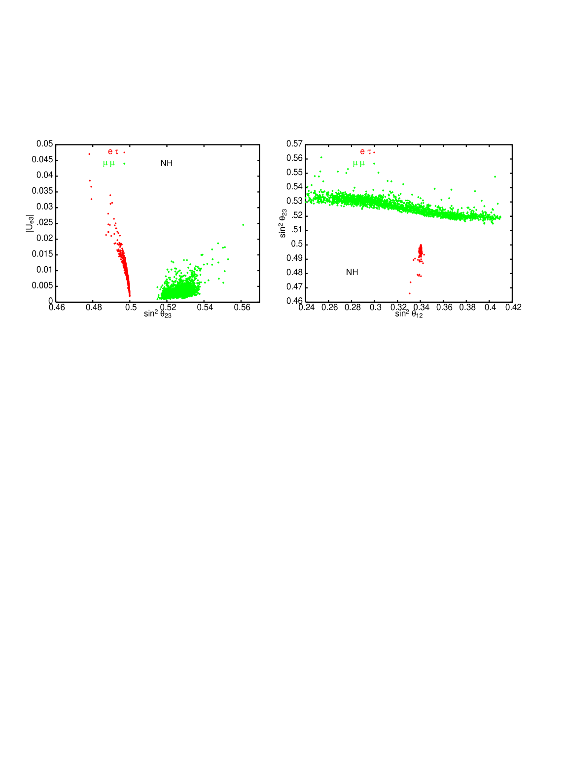
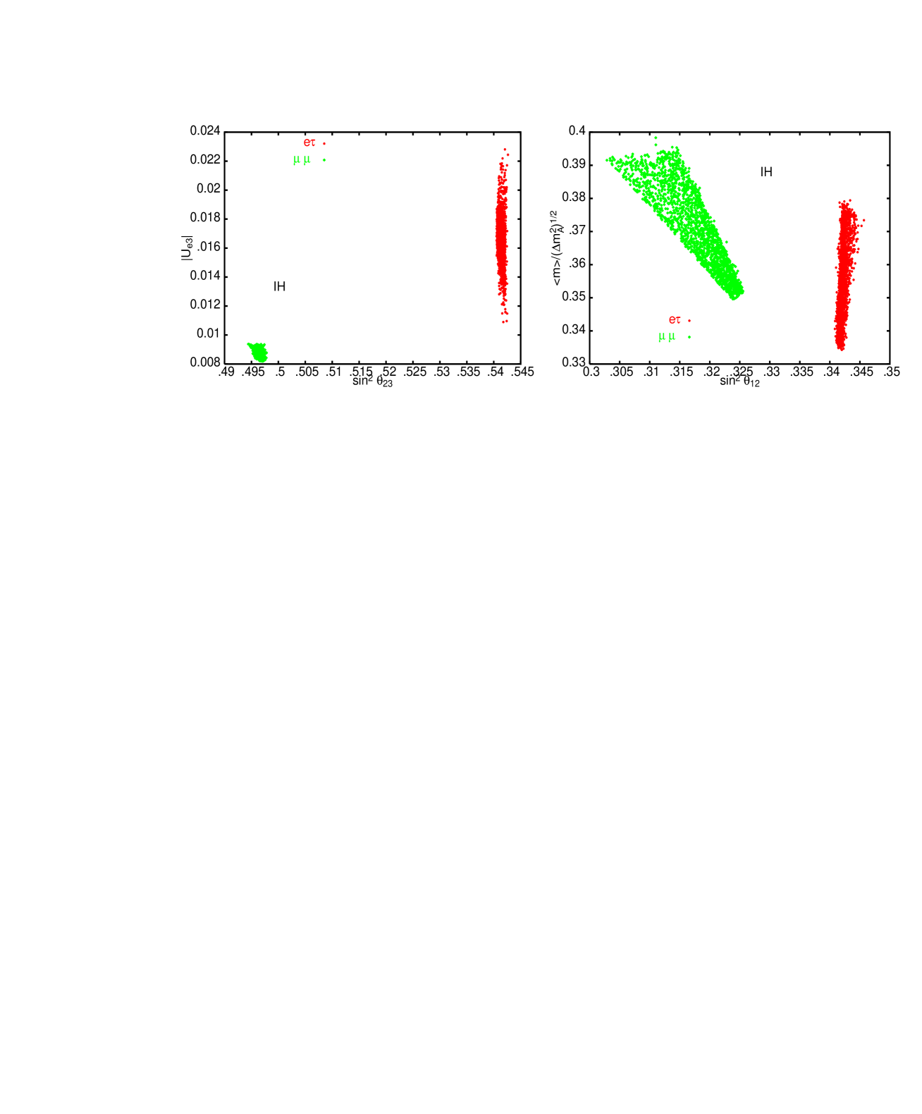
Figure 1: Scatter plots of some of the correlations of the observables for the normal hierarchy resulting from Eqs. (7) and (10). The parameters $A,B,D$ are complex and $|A|,|B|$ are smaller than $D$ by one order of magnitude. The dark (red) points are for a perturbation in the $e\tau$ element, the bright (green) points for a perturbation in the $\mu\mu$ element.

Figure 2: Same as above for the inverted hierarchy. We have now $|D|$ smaller than $|A|,|B|$ by one order of magnitude and $|A|\simeq|B/2|$.

References

- [1] S. T. Petcov, Nucl. Phys. Proc. Suppl. 143, 159 (2005), hep-ph/0412410.
- [2] B. Pontecorvo, Zh. Eksp. Teor. Fiz. 33, 549 (1957) and 34, 247 (1958); Z. Maki, M. Nakagawa and S. Sakata, Prog. Theor. Phys. 28, 870 (1962).
- [3] S. M. Bilenky, J. Hosek and S. T. Petcov, Phys. Lett. B 94, 495 (1980); M. Doi et al., Phys. Lett. B 102, 323 (1981); J. Schechter and J. W. F. Valle, Phys. Rev. D 23, 1666 (1981).
- [4] M. Maltoni et al., New J. Phys. 6, 122 (2004), hep-ph/0405172v4.
- [5] The values for and have been obtained by A. Bandyopadhyay, S. Choubey and S. Goswami by updating the analysis from A. Bandyopadhyay et al., Phys. Lett. B 608, 115 (2005) with the latest SNO results.
- [6] For recent reviews see, e.g., S. F. King, Rept. Prog. Phys. 67, 107 (2004); G. Altarelli and F. Feruglio, New J. Phys. 6, 106 (2004); R. N. Mohapatra et al., hep-ph/0412099.
- [7] P. F. Harrison, D. H. Perkins and W. G. Scott, Phys. Lett. B 458, 79 (1999); Phys. Lett. B 530, 167 (2002); P. F. Harrison and W. G. Scott, Phys. Lett. B 535, 163 (2002); Phys. Lett. B 557, 76 (2003); X. G. He and A. Zee, Phys. Lett. B 560, 87 (2003); E. Ma, Phys. Rev. Lett. 90, 221802 (2003); Phys. Lett. B 583, 157 (2004); C. I. Low and R. R. Volkas, Phys. Rev. D 68, 033007 (2003); S. H. Chang, S. K. Kang and K. Siyeon, Phys. Lett. B 597, 78 (2004); E. Ma, Phys. Rev. D 70, 031901 (2004); F. Caravaglios and S. Morisi, hep-ph/0503234; G. Altarelli, F. Ferruglio, hep-ph/0504165; E. Ma, hep-ph/0505209; I. de Medeiros Varzielas and G. G. Ross, hep-ph/0507176; K. S. Babu and X. G. He, hep-ph/0507217.
- [8] A. Zee, Phys. Rev. D 68, 093002 (2003); N. Li and B. Q. Ma, Phys. Rev. D 71, 017302 (2005).
- [9] Z. Z. Xing, Phys. Lett. B 533, 85 (2002).
- [10] S. F. King, hep-ph/0506297.
- [11] L. Wolfenstein, Phys. Rev. D 18, 958 (1978).
- [12] B. Aharmim et al. [SNO Collaboration], nucl-ex/0502021.
- [13] S. Choubey and W. Rodejohann, hep-ph/0506102; S. Goswami, talk given at XXII International Symposium on Lepton–Photon Interactions at High Energy ”Lepton/Photon 05”, Uppsala, Sweden, July 2005; http://lp2005.tsl.uu.se/ lp2005/LP2005/programme/index.htm
- [14] P. Huber et al., Phys. Rev. D 70, 073014 (2004).
- [15] J. N. Bahcall and C. Pena-Garay, JHEP 0311, 004 (2003).
- [16] A. Bandyopadhyay et al., hep-ph/0410283.
- [17] F. Vissani, hep-ph/9708483; V. D. Barger, S. Pakvasa, T. J. Weiler and K. Whisnant, Phys. Lett. B 437, 107 (1998); A. J. Baltz, A. S. Goldhaber and M. Goldhaber, Phys. Rev. Lett. 81, 5730 (1998); H. Georgi and S. L. Glashow, Phys. Rev. D 61, 097301 (2000); I. Stancu and D. V. Ahluwalia, Phys. Lett. B 460, 431 (1999).
- [18] C. S. Lam, Phys. Lett. B 507, 214 (2001); W. Grimus and L. Lavoura, JHEP 0107, 045 (2001); Eur. Phys. J. C 28, 123 (2003); J. Phys. G 30, 1073 (2004); T. Kitabayashi and M. Yasue, Phys. Lett. B 524, 308 (2002); I. Aizawa et al., Phys. Rev. D 70, 015011 (2004); W. Grimus et al., JHEP 0407, 078 (2004); R. N. Mohapatra, S. Nasri and H. B. Yu, Phys. Lett. B 615, 231 (2005); R. N. Mohapatra and S. Nasri, Phys. Rev. D 71, 033001 (2005); C. S. Lam, Phys. Rev. D 71, 093001 (2005).
- [19] P. F. Harrison and W. G. Scott, Phys. Lett. B 547, 219 (2002); E. Ma, Phys. Rev. D 66, 117301 (2002); I. Aizawa, T. Kitabayashi and M. Yasue, hep-ph/0504172; T. Kitabayashi and M. Yasue, hep-ph/0504212.
- [20] W. Grimus et al., Nucl. Phys. B 713, 151 (2005).
- [21] P. Binetruy et al., Nucl. Phys. B 496, 3 (1997); N. F. Bell and R. R. Volkas, Phys. Rev. D 63, 013006 (2001); S. Choubey and W. Rodejohann, Eur. Phys. J. C 40, 259 (2005).
- [22] K. S. Babu, E. Ma and J. W. F. Valle, Phys. Lett. B 552, 207 (2003); M. Hirsch et al., Phys. Rev. D 69, 093006 (2004).
- [23] R. N. Mohapatra, JHEP 0410, 027 (2004).
- [24] See for instance S. Antusch et al., JHEP 0503, 024 (2005) and references therein.
- [25] M. Jezabek and Y. Sumino, Phys. Lett. B 457, 139 (1999); Z. Z. Xing, Phys. Rev. D 64, 093013 (2001); C. Giunti and M. Tanimoto, Phys. Rev. D 66, 053013 (2002); Phys. Rev. D 66, 113006 (2002); W. Rodejohann, Phys. Rev. D 69, 033005 (2004); G. Altarelli, F. Feruglio and I. Masina, Nucl. Phys. B 689, 157 (2004); A. Romanino, Phys. Rev. D 70, 013003 (2004).
- [26] M. Raidal, Phys. Rev. Lett. 93, 161801 (2004); H. Minakata and A. Y. Smirnov, Phys. Rev. D 70, 073009 (2004); P. H. Frampton and R. N. Mohapatra, JHEP 0501, 025 (2005); J. Ferrandis and S. Pakvasa, Phys. Rev. D 71, 033004 (2005); N. Li and B. Q. Ma, Phys. Rev. D 71, 097301 (2005); hep-ph/0504161; S. K. Kang, C. S. Kim and J. Lee, hep-ph/0501029; K. Cheung et al., hep-ph/0503122; Z. Z. Xing, hep-ph/0503200; A. Datta, L. Everett and P. Ramond, hep-ph/0503222; S. Antusch, S. F. King and R. N. Mohapatra, hep-ph/0504007; H. Minakata, hep-ph/0505262; T. Ohlsson, hep-ph/0506094.
- [27] P. H. Frampton, S. T. Petcov and W. Rodejohann, Nucl. Phys. B 687, 31 (2004); S. T. Petcov and W. Rodejohann, Phys. Rev. D 71, 073002 (2005).
- [28] C. Jarlskog, Z. Phys. C 29, 491 (1985); Phys. Rev. D 35, 1685 (1987).
- [29] P. I. Krastev and S. T. Petcov, Phys. Lett. B 205 (1988) 84.
- [30] J. F. Nieves and P. B. Pal, Phys. Rev. D 36, 315 (1987); Phys. Rev. D 64, 076005 (2001); J. A. Aguilar-Saavedra and G. C. Branco, Phys. Rev. D 62, 096009 (2000).