MSU-HEP-050707

Abstract. I present an overview of some current topics in the measurement of Parton Distribution Functions.

1 Introduction

Parton distribution functions describe the quark and gluon content of a hadron when the parton-parton correlations and spin structure have been integrated out. By the asymptotic freedom of QCD, the PDFs are the only aspect of initial-state hadron structure that is needed to calculate short-distance hard scattering. Hence PDFs are a Fundamental Measurement: a challenge to understand using methods of nonperturbative QCD; and a Necessary Evil: essential input to perturbative calculations of signal and background at hadron colliders.

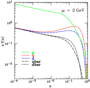
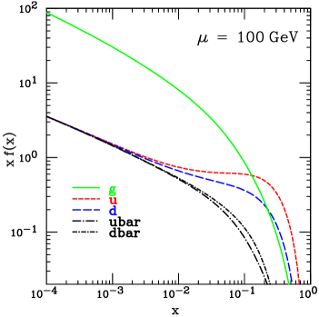
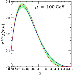
The parton distributions are functions $f_{a}(x,\mu)$ that tell the probability density for a parton of flavor $a$ in a proton or other hadron, at momentum fraction $x$ and momentum scale $\mu$. An overview is shown in Fig. 1 at $\mu=2\,\mathrm{GeV}$ and $\mu=100\,\mathrm{GeV}$. Valence quarks dominate at $x\to 1$, while gluons dominate at small $x$, especially at large $\mu$—hence their vital importance for the LHC.

The PDFs are measured through a “global analysis” in which a large variety of data from many experiments that probe short distance are fitted simultaneously. The full paradigm consists of the following steps:

1. Parameterize the $x$-dependence for each flavor at a fixed small $\mu_{0}$, using functional forms that contain “shape parameters” $A_{1},\dots,A_{N}$.

2. Compute the PDFs $f_{a}(x,\mu)$ at $\mu>\mu_{0}$ by the DGLAP equation.

3. Compute the cross sections for DIS($e$,$\mu$,$\nu$), Drell-Yan, Inclusive jets, etc. by perturbation theory.

4. Compute the “$\chi^{2}$” measure of agreement between the predictions and experiment:

   $$\chi^{2}=\sum_{i}\left(\frac{\mathrm{Data}_{i}-\mathrm{Theory}_{i}}{\mathrm{Error}_{i}}\right)^{2}$$

   or generalizations of that formula to include correlated experimental errors.

5. Minimize $\chi^{2}$ with respect to the parameters $\{A_{i}\}$ to obtain Best Fit PDFs.

6. Map the PDF uncertainty range as the region in $\{A_{i}\}$ space where $\chi^{2}$ is sufficiently close to the minimum.

7. Make the best fit and uncertainty sets available at http://durpdg.dur.ac.uk/HEPDATA/. At that site, you can find the current CTEQ, MRST, Alekhin, H1, and ZEUS sets, along with some older CTEQ, MRST, and GRV sets.

Figure 1: Overview of PDF results from CTEQ6.

The global analysis rests on three solid theoretical pillars:

1. Asymptotic Freedom $\Rightarrow$ QCD interactions are weak at large scale $\mu$ (short distance), so a perturbative expansion in powers of $\alpha_{s}(\mu)$ at NLO or NNLO can be used to make the calculations;

2. Factorization Theorem $\Rightarrow$ PDFs are universal, i.e., the same for all processes;

3. DGLAP evolution $\Rightarrow$ the dependence of $f_{a}(x,\mu)$ on momentum scale $\mu$ is perturbatively calculable, so only the dependence on light-cone momentum fraction $x$ for each flavor $a$ at a fixed small $\mu_{0}$ needs to be measured.

Carrying out the global analysis brings a constant battle against the following challenges:

• Extracting continuous functions from a finite set of measurements is mathematically unclean. In particular, the analysis is carried out by modeling the PDFs at $\mu_{0}$ by smooth functions containing free parameters. The bias that can result from the choice of these functional forms is known as “parametrization dependence.”

• A specific type of parametrization dependence consists of simplifying assumptions that are made in the absence of data, such as strangeness symmetry ($f_{s}(x,\mu_{0})=f_{\bar{s}}(x,\mu_{0})$) which was assumed in most older analyses; or the condition of no intrinsic charm ($f_{c}(x,m_{c})=f_{\bar{c}}(x,m_{c})=0$) which is still used.

• Combining data from diverse experiments is frequently made difficult by the presence of unknown errors. This is true even when a single discrete quantity like the mass or lifetime of a particle is measured; but the situation is worse when one is attempting to measure a large number of parameters (the $\{A_{i}\}$) from many experiments that are sensitive to different combinations of those parameters.

• The quality of the fit to data is measured—by tradition and because there is no obvious better alternative—by a global $\chi^{2}$ that is based on the reported experimental errors. But unquantified experimental and theoretical systematic errors are found to be almost an order of magnitude larger, based on the level of inconsistencies observed between the “pulls” of various data sets, so the reported experimental errors do not really provide the ideal weighting of the data points.

2 The landscape in $x$ and $\mu$

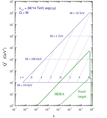
The kinematic regions of interest in $x$ and $\mu$ are shown in Fig. 2 (lifted from a talk by James Stirling). One sees that a large range of scales in $\mu$ are connected by DGLAP evolution. The consistency or inconsistency between the different processes that make up the global analysis can be tested only by the global fit, since every experiment depends differently on the PDFs. The LHC will dramatically extend the region of the measurements and their applications—especially at small $x$.

Figure 2: Kinematic map in $x$ and $Q\equiv\mu$.

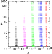
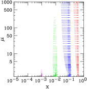
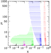
The DGLAP evolution in $\mu$ arises from parton branching, so the PDFs at a given $x$ and $\mu$ can be thought of as arising from PDFs at smaller $\mu$ and larger $x$. To develop a feel for how this works quantitatively, Fig. 3 shows the regions where one or more of the PDFs changes by $>\!0.2\,\%$ (solid) or $>\!0.05\,\%$ (dotted) when a $1\%$ change is made in $\bar{u}+\bar{d}$ or $u_{v}\equiv u-\bar{u}$ or $g$ at $\mu_{0}=1.3\,\mathrm{GeV}$ in a narrow band of $x$ at various values of $x$. One sees that the valence quarks are unimportant at small $x$—as expected—and that quark evolution is effectively at constant $x$, i.e., the quark distributions at a given $x$ and $\mu$ are mainly influenced by the quarks at $\mu_{0}$ at the same $x$. The gluon at very large $x$ similarly evolves in its own world. But the influence of changes in the input $g(x)$ at moderate $x$ spreads out rapidly. The small-$x$ gluon at $\mu_{0}=1.3\,\mathrm{GeV}$ has little direct influence because gluons at moderate and high $\mu$ are mainly generated radiatively.

Figure 3: Regions of change caused by small changes in $\bar{u}(x)+\bar{d}(x)$ (left) or $u_{v}(x)$ (center) or $g(x)$ (right) at $\mu=1.3\,\mathrm{GeV}$ and $x=10^{-4}$, $10^{-3}$, $10^{-2}$, $10^{-1}$, $0.4\,$.

3 PDF uncertainties

A large effort has been made in recent years to intelligently consider the uncertainties of PDF measurements. This is a more difficult problem than most other error estimates because the objects are functions, rather than discrete values; and because they are extracted from a complicated stew of experiments of different types. Obvious sources of uncertainty are

1. Experimental errors included in $\chi^{2}$

2. Unknown experimental errors and theory approximations

3. Higher-order QCD corrections $+$ Large Logs

4. Power Law QCD corrections (“higher twist”)

5. Parametrization dependence

6. Nuclear corrections for data that are taken on deuterium or other nuclear targets.

Essential difficulties arise from the fact that

• Experiments run until systematic errors dominate, so the remaining systematic error estimates involve guesswork.

• The systematic errors of the theory (e.g. power-law corrections or the approximations of NLO or NNLO) and their correlations are even harder to guess.

• Some combinations of PDFs are unconstrained, like $s\!-\!\bar{s}$ was before the NuTeV data.

Figure 4: Hypothetical measurements of a quantity $\theta$ by two experiments.

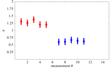
Empirically, the essence of the uncertainty problem is illustrated by the hypothetical Figure 4. Suppose the quantity $\theta$ is measured in two different experiments. What would you quote as the central value and the uncertainty? (To play along at home, write down your answer before reading further!) Perhaps you would expand the errors to make the uncertainty range cover both data sets. Or perhaps you would expand it even more, using the difference between experiments as a measure of the uncertainty. Perhaps you would also be suspicious that the spread in the points from each experiment is too small compared to the quoted errors.

In the global analysis, we don’t get to see the conflicts so directly as in Figure 4. But if you make a best fit to the points in Figure 4 with different weights assigned to the two experiments, the variation of the best fit value with the choice of weights would map out the information that is needed. That approach can be used in the global fit. In practice to quantify the uncertainties of the PDF global fit, we retain $\chi^{2}$ as the measure of fit quality, but vary weights of the experiments to estimate a range of acceptable $\Delta\chi^{2}$ above the minimum value, in place of the classical $\Delta\chi^{2}=1$. Estimates for the current major global analyses are that something like $\Delta\chi^{2}=50-100$ corresponds to a $\sim 90\%$ confidence interval.

4 Eigenvector uncertainty sets

A convenient way to characterize the uncertainty of the PDFs is to create a collection of fits by stepping away from the minimum of $\chi^{2}$ along each eigenvector direction of the quadratic form (the Hessian matrix) that describes the dependence of $\chi^{2}$ on the fitting parameters $\{A_{i}\}$ in the neighborhood of the minimum. This stepping is done in both directions along each eigenvector to allow asymmetric errors, so the 20 fitting parameters in CTEQ6 lead to 40 eigenvector uncertainty sets. The PDF uncertainty for any quantity is obtained by evaluating that quantity with each of the eigenvector sets and then applying a simple formula; or more crudely just directly from the spread in eigenvector predictions. This method has proven so useful that generating uncertainty sets should be regarded as an essential part of the job for every general-purpose PDF determination. In order to do this properly, CTEQ has developed an iterative procedure [1] to compute the eigenvector directions in the face of numerical instabilities that arise from the large dynamic range in eigenvalues of the Hessian. (Other PDF groups have adopted the eigenvector method as well, but they avoid the numerical difficulties by keeping substantially fewer free fitting parameters, e.g. $10-15$, at a cost of greater parametrization bias.)

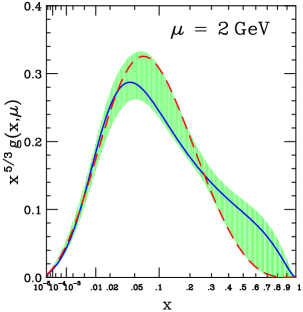
The uncertainty of the gluon distribution at $\mu=2\,\mathrm{GeV}$, as calculated by the eigenvector method, is shown in Fig. 5. Also shown are best fits in which the data were reweighted to emphasize DØ (solid) or CDF (dashed) inclusive jet cross section measurements. Note that the uncertainty estimated by the eigenvector method is comparable to the difference between the “pull” of these two experiments. This shows that the eigenvector method is working correctly, and that the jet data are a major source of the information on the gluon distribution.

It is interesting that these two very similar experiments pull so differently, which suggests that the need to allow $\Delta\chi^{2}\gg 1$ may be mainly due to unknown systematic errors in the experiments. (In support of that notion, we also find significant differences between the influences of the nominally similar H1 and ZEUS components of DIS data.)

The right-hand side of Fig. 5 demonstrates “convergent evolution:” the fractional uncertainty of the gluon is much smaller at large $\mu$.

Figure 5: Gluon uncertainty at $\mu=2\,\mathrm{GeV}$ and $\mu=100\,\mathrm{GeV}$ from CTEQ6, plotted vs. $x^{1/3}$. Solid (dashed) curve has extra weight for DØ (CDF) jet data.

5 PDF comparisons

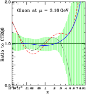
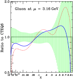
The fractional uncertainty of the gluon distribution at an intermediate scale $\mu=3.16\,\mathrm{GeV}$ relative to CTEQ6 is shown in the left panel of Fig. 6. The dotted curve is CTEQ5, the previous generation of CTEQ PDFs. The dashed curve is CTEQ5HJ, which was an early milestone in the PDF uncertainty business: it accounted for the seemingly high CDF inclusive jet cross section, relative to the QCD prediction, by an increased gluon distribution at large $x$ that was well within the PDF uncertainty range. The solid curve is CTEQ6.1, which shows very little change from CTEQ6.0.

Figure 6: Gluon uncertainty at $\mu^{2}=10\,\mathrm{GeV}^{2}$ relative to cteq6. Left: cteq5 (dotted), cteq5HJ (dashed) and cteq6.1 (solid); Center: zeus2005zj (solid), Alekhin02NLO (long dash) and Alekhin02NNLO (short dash); Right: mrst2001 (dotted), mrst2002 (short dash), mrst2003 (long dash), mrst2004 (solid).

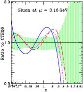
The center panel of Figure 6 shows a comparison with fits by the ZEUS group and by Alekhin. Since those fits are based on only a subset of the available data used in the CTEQ analysis, it is not surprising that they lie outside the CTEQ uncertainty bands. The difference between the Alekhin NLO (long dash) and NNLO (short dash) is seen to be small compared to the PDF uncertainty.

The right panel of Figure 6 shows a comparison with fits by the MRST group. The MRST fits have progressed toward a stronger gluon at large $x$, which is needed to obtain good fits to the inclusive jet cross sections. The small-$x$ behavior is sensitive to parametrization assumptions that will be discussed later.

It is ironic that the differences between PDF determinations by the various major players are comparable to the estimated uncertainty. For our original motivation to study the uncertainties systematically was the danger that comparing results from different groups might greatly underestimate the uncertainty, since all groups use basically the same method.

6 NLO and NNLO

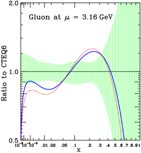
Figure 7 shows a comparison with NLO and NNLO fits by the MRST group. At present, the difference between NLO and NNLO analysis is small compared to the PDF uncertainty. This is also apparent in the Alekhin fits shown in Fig. 6. Hence NNLO fitting, while obviously desirable on theoretical grounds, is not urgent. A reasonable goal would be to have a full set of NNLO global analysis tools—including jet cross sections—in place by the time LHC data taking begins.

Figure 7: Showing that NNLO effects are small for the PDFs: Left is mrst2002 NLO (solid) and NNLO (dotted); Right is mrst2004 NLO (solid) and NNLO (dotted).

7 Negative gluons and the stability of NLO

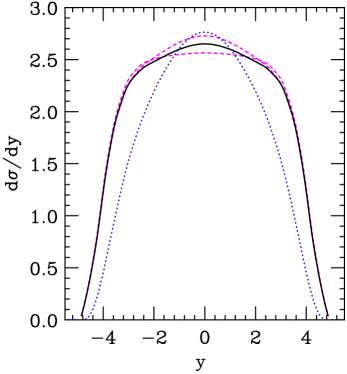
It has been hoped that the $W^{\pm}$ production cross section can be used as a “Standard Candle” to measure parton luminosity at the LHC. But a challenge to the belief that $\sigma_{W}$ can be reliably predicted arose with the mrst2003c PDFs. The ‘c’ label refers to ‘conservative’ cuts ($x>0.005$, $Q>3.162\,\mathrm{GeV}$) on the input data set to avoid possible contamination from physics that is missing in the NLO analysis. But—as sometimes also happens in politics—this “conservative” approach led to a “radical” outcome: a much smaller predicted cross section.

The origin of the surprising prediction is a preference of the MRST fit for a much smaller gluon distribution at small $x$, which is associated with $g(x,\mu)$ actually turning negative, even at a momentum scale as large as $\mu=m_{W}$. This suppresses the predicted $d\sigma/dy$ for $W^{+}+W^{-}$ at large $|y|$ as shown in Fig. 8.

In agreement with MRST, CTEQ finds that negative gluon PDFs can produce an acceptable fit to the data with the conservative cuts, while predicting a small $d\sigma/dy$ similar to that of mrst2003c. But in disagreement with MRST, CTEQ finds the NLO fits to be stable with respect to variations in the cuts, which leaves no persuasive motivation to make the “conservative” cuts. The disagreement appears to arise from parametrization assumptions, since in the latest MRST NLO fit (mrst2004nlo) a different ansatz for the gluon distribution at $\mu_{0}$ has led to a different small-$x$ behavior. For details, see [2] and Dan Stump’s talk at this conference.

Figure 8: Predicted rapidity distribution for $W^{+}\!+\!W^{-}$ at the LHC: cteq6.1 (solid); cteq6.1 uncertainty range (dashed); mrst2003cnlo (dotted).

8 New Physics from PDF fits?

Figure 9: Contour plot of $\chi^{2}-\chi^{2}_{\mathrm{CTEQ6}}$ vs. $M_{\tilde{g}}$ and $\alpha_{s}(M_{Z})$.

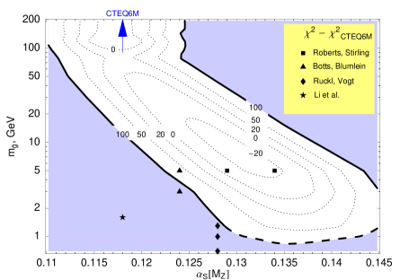
The global fit for PDFs relies on lots of Standard Model QCD, so the quality of the fit can be sensitive to Beyond Standard Model physics. As a specific example, the existence of a light gluino would modify PDF evolution and jet production [3]. A contour plot of $\chi^{2}-\chi^{2}_{\mathrm{CTEQ6}}$ vs. $M_{\tilde{g}}$ and $\alpha_{s}(M_{Z})$ is shown in Fig. 9. There is a valley at $5\,\mathrm{GeV}<M_{\tilde{g}}<20\,\mathrm{GeV}$ with a depth of $\Delta\chi^{2}\approx-25$, which could be regarded by a SUSY fanatic as a hint for a light gluino. But a more down-to-earth interpretation is simply as a confirmation of the Standard Model, along with further evidence that a change of at least $50-100$ in $\chi^{2}$ is necessary to signal a persuasive change in the quality of the current fits.

9 The future

We can expect to see steady progress in the field of parton distribution measurements during the final productive years of HERA and the Tevatron, followed by dramatic developments when LHC data become available.

At the present time, there are a number of improvements underway from the theory side:

• Improved treatment of heavy quarks.

• Complete NNLO calculations.

• Weaker input assumptions.

With regard to the input assumptions, one way to eliminate possible biases caused by a choice of functional forms for the PDfs at $\mu_{0}$ was discussed at this conference: to replace the parametrizations by neural net methods [4]. Work is underway to open up the assumptions on strangeness: in previous analyses, $s+\bar{s}\propto\bar{d}+\bar{u}$ has been assumed. Work is also underway to allow for possible nonradiatively generated (i.e., “intrinsic”) $c,\,\bar{c}$ and $b,\,\bar{b}$. At the same time, it is worthwhile to look at possibilities for making stronger input assumptions, by incorporating ideas from nonperturbative models or lattice calculations.

There will also be many improvements in the input data set in the near future:

• H1 and ZEUS are taking much more data.

• NuTeV data analysis at NLO is in progress.

• E866 final data are nearly ready.

• CDF and DØ will have improved measurements of inclusive jets and the lepton rapidity asymmetry from W decay.

There are some new types of measurement that could be made at HERA which would be useful for improving the determination of PDFs. Most importantly, they could measure $F_{L}$, though it will require them to accept the risk of using part of their remaining running time to switch to a lowered proton energy. Perhaps that risk is actually not so large, since the small increase in statistics to be gained by say the last half year of conventional running is not all that valuable. In a more perfect world, it would also be very nice if HERA would measure DIS on deuterium.

CDF and DØ can also make major new contributions through measurements of

• Inclusive $Z^{0}$ and $W^{\pm}$ .

• Inclusive jet with $c$- or $b$-tag.

• $\gamma/Z^{0}/W^{\pm}$ + jet with $c$- or $b$-tag.

Some data has already been reported for $Z^{0}$+bjet (DØ) [5] and $\gamma$+bjet (CDF) [6]. For more information on these and other possibilities, see the proceedings of the HeraLHC [7] and TeV4LHC [8] workshops.

Principal efforts in the application of parton distributions in the near term will be to the difficult question of systematic errors of the $W$ mass measurement at the Tevatron, and to All Things LHC—the Standard Model and beyond. It is also worthwhile to mention that important extensions of the PDF approach are going on to study (1) Spin-dependent PDFs, (2) transverse momentum dependent “generalized” PDFs, and (3) parton distributions of nuclei.

Acknowledgements:

I wish to thank the organizers for an excellent conference. I thank Robert Thorne, Stan Brodsky, Wu-Ki Tung, Dan Stump, and Joey Huston for many discussions. This work is supported by the National Science Foundation.

References

- [1] J. Pumplin et al., Phys. Rev. D 65, 014011 (2002) [arXiv:hep-ph/0008191].
- [2] J. Huston, et al., “Stability of NLO global analysis and implications for hadron collider physics,” [arXiv:hep-ph/0502080] to be published in JHEP.
- [3] E. L. Berger, et al., Phys. Rev. D 71, 014007 (2005) [arXiv:hep-ph/0406143].
- [4] J. Rojo et al., “The neural network approach to parton fitting,” [arXiv:hep-ph/0505044] and talk at this conference.
- [5] V. M. Abazov et al., Phys. Rev. Lett. 94, 161801 (2005).
- [6] Reported by Amnon Harel at this conference.
- [7] http://www.desy.de/ heralhc/
- [8] http://conferences.fnal.gov/tev4lhc/