1 Introduction

Effective Field Theories (EFTs) are the counterpart of the Theory of Everything. They are the field theoretical implementation of the quantum ladder: heavy degrees of freedom need not be included among the quantum fields of an EFT for a description of low-energy phenomena. For example, we do not need quantum gravity to understand the hydrogen atom nor does chemistry depend upon the structure of the electromagnetic interaction of quarks.

EFTs are approximations by their very nature. Once the relevant degrees of freedom for the problem at hand have been established, the corresponding EFT is usually treated perturbatively. It does not make much sense to search for an exact solution of the Fermi theory of weak interactions. In the same spirit, convergence of the perturbative expansion in the mathematical sense is not an issue. The asymptotic nature of the expansion becomes apparent once the accuracy is reached where effects of the underlying “fundamental” theory cannot be neglected any longer. The range of applicability of the perturbative expansion depends on the separation of energy scales that define the EFT.

EFTs pervade much of modern physics. The effective nature of the description is evident in atomic and condensed matter physics. The following article will be restricted to particle physics where EFTs have become important tools during the last 25 years.

2 Classification of effective field theories

A first classification of EFTs is based on the structure of the transition from the “fundamental” (energies $>\Lambda$) to the “effective” level (energies $<\Lambda$).

1. Complete decoupling.
   The fundamental theory contains heavy and light degrees of freedom. Under very general conditions (decoupling theorem, Appelquist and Carazzone, 1975), the effective Lagrangian for energies $\ll\Lambda$, depending only on light fields, takes the form

   $${\cal L}_{\rm eff}={\cal L}_{d\leq 4}+\sum_{d>4}\frac{1}{\Lambda^{d-4}}\sum_{i_{d}}g_{i_{d}}O_{i_{d}}~{}.$$ (1)

   The heavy fields with masses $>\Lambda$ have been “integrated out” completely. ${\cal L}_{d\leq 4}$ contains the potentially renormalizable terms with operator dimension $d\leq 4$ (in natural mass units where Bose and Fermi fields have $d=1$ and 3/2, respectively), the $g_{i_{d}}$ are coupling constants and the $O_{i_{d}}$ are monomials in the light fields with operator dimension $d$. In a slightly misleading notation, ${\cal L}_{d\leq 4}$ consists of relevant and marginal operators whereas the $O_{i_{d}}~{}(d>4)$ are denoted irrelevant operators. The scale $\Lambda$ can be the mass of a heavy field (e.g., $M_{W}$ in the Fermi theory of weak interactions) or it reflects the short-distance structure in a more indirect way.

2. Partial decoupling.
   In contrast to the previous case, the heavy fields do not disappear completely from the EFT but only their high-momentum modes are integrated out. The main area of application is the physics of heavy quarks (Sec. 4). The procedure involves one or several field redefinitions introducing a frame dependence. Lorentz invariance is not manifest but implies relations between coupling constants of the EFT (reparametrization invariance).

3. Spontaneous symmetry breaking.
   The transition from the fundamental to the effective level occurs via a phase transition due to spontaneous symmetry breaking generating (pseudo-)Goldstone bosons. A spontaneously broken symmetry relates processes with different numbers of Goldstone bosons. Therefore, the distinction between renormalizable ($d\leq 4$) and nonrenormalizable ($d>4$) parts in the effective Lagrangian (1) becomes meaningless. The effective Lagrangian of type 3 is generically nonrenormalizable. Nevertheless, such Lagrangians define perfectly consistent quantum field theories at sufficiently low energies. Instead of the operator dimension as in (1), the number of derivatives of the fields and the number of symmetry breaking insertions distinguish successive terms in the Lagrangian. The general structure of effective Lagrangians with spontaneously broken symmetries is largely independent of the specific physical realization (universality). There are many examples in condensed matter physics but the two main applications in particle physics are electroweak symmetry breaking (Sec. 3.2) and chiral perturbation theory (Secs. 5.1,5.2) with the spontaneously broken global chiral symmetry of QCD.

Another classification of EFTs is related to the status of their coupling constants.

1. Coupling constants can be determined by matching the EFT with the underlying theory at short distances.
   The underlying theory is known and Green functions can be calculated perturbatively at energies $\sim\Lambda$ both in the fundamental and in the effective theory. Identifying a minimal set of Green functions fixes the couplings constants $g_{i_{d}}$ in Eq. (1) at the scale $\Lambda$. Renormalization group equations can then be used to run the couplings down to lower scales. The nonrenormalizable terms in the Lagrangian (1) can be fully included in the perturbative analysis.

2. Coupling constants are constrained by symmetries only.

   • The underlying theory and therefore also the EFT coupling constants are unknown. This is the case of the SM (Sec. 3). A perturbative analysis beyond leading order only makes sense for the known renormalizable part ${\cal L}_{d\leq 4}$. The nonrenormalizable terms suppressed by powers of $\Lambda$ are considered at tree level only. The associated coupling constants $g_{i_{d}}$ serve as bookmarks for new physics. Usually, but not always (cf., e.g., Sec. 3.1), the symmetries of ${\cal L}_{d\leq 4}$ are assumed to constrain the couplings.

   • The matching cannot be performed in perturbation theory even though the underlying theory is known. This is the generic situation for EFTs of type 3 involving spontaneous symmetry breaking. The prime example is chiral perturbation theory as the EFT of QCD at low energies.

3 The Standard Model as an EFT

With the possible exception of the scalar sector to be discussed in Sec. 3.2, the SM is very likely the renormalizable part of an EFT of type 1 B. Except for nonzero neutrino masses, the SM Lagrangian ${\cal L}_{d\leq 4}$ in (1) accounts for physics up to energies of roughly the Fermi scale $G_{F}^{-1/2}\simeq 300$ GeV.

Since the SM works exceedingly well up to the Fermi scale where the electroweak gauge symmetry is spontaneously broken it is natural to assume that the operators $O_{i_{d}}$ with $d>4$, made up from fields representing the known degrees of freedom and including a single Higgs doublet in the SM proper, should be gauge invariant with respect to the full SM gauge group $SU(3)_{c}\times SU(2)_{L}\times U(1)_{Y}$. An almost obvious constraint is Lorentz invariance that will be lifted in Sec. 3.1, however.

These requirements limit the Lagrangian with operator dimension d=5 to a single term (except for generation multiplicity), consisting only of a left-handed lepton doublet $L_{L}$ and the Higgs doublet $\Phi$:

$$O_{d=5}=\epsilon_{ij}\epsilon_{kl}L_{iL}^{\top}C^{-1}L_{kL}\Phi_{j}\,\Phi_{l}+~{}{\rm h.c.}$$ (2)

This term violates lepton number and generates nonzero Majorana neutrino masses. For a neutrino mass of 1 eV, the scale $\Lambda$ would have to be of the order of $10^{13}$ GeV if the associated coupling constant in the EFT Lagrangian (1) is of order 1.

In contrast to the simplicity for d=5, the list of gauge invariant operators with d=6  is enormous. Among them are operators violating baryon or lepton number that must be associated with a scale much larger than 1 TeV. To explore the territory close to present energies, it therefore makes sense to impose baryon and lepton number conservation on the operators with d=6. Those operators have all been classified (Buchmüller and Wyler, 1986) and the number of independent terms is of the order of 80. They can be grouped in three classes.

The first class consists of gauge and Higgs fields only. The corresponding EFT Lagrangian has been used to parametrize new physics in the gauge sector constrained by precision data from LEP. The second class consists of operators bilinear in fermion fields, with additional gauge and Higgs fields to generate d=6. Finally, there are 4-fermion operators without other fields or derivatives. Some of the operators in the last two groups are also constrained by precision experiments, with a certain hierarchy of limits. For lepton and/or quark flavour conserving terms, the best limits on $\Lambda$ are in the few TeV range whereas the absence of neutral flavour changing processes yields lower bounds on $\Lambda$ that are several orders of magnitude larger. If there is new physics in the TeV range flavour changing neutral transitions must be strongly suppressed, a powerful constraint on model building.

It is amazing that the most general renormalizable Lagrangian with the given particle content accounts for almost all experimental results in such an impressive manner. Finally, we recall that many of the operators of dimension 6 are also generated in the SM via radiative corrections. A necessary condition for detecting evidence for new physics is therefore that the theoretical accuracy of radiative corrections matches or surpasses the experimental precision.

3.1 Noncommutative space-time

Noncommutative geometry arises in some string theories and may be expected on general grounds when incorporating gravity into a quantum field theory framework. The natural scale of noncommutative geometry would be the Planck scale in this case without observable consequences at presently accessible energies. However, as in theories with large extra dimensions the characteristic scale $\Lambda_{\rm NC}$ could be significantly smaller. In parallel to theoretical developments to define consistent noncommutative quantum field theories (short for quantum field theories on noncommutative space-time), a number of phenomenological investigations have been performed to put lower bounds on $\Lambda_{\rm NC}$.

Noncommutative geometry is a deformation of ordinary space-time where the coordinates, represented by hermitian operators $\hat{x}_{\mu}$, do not commute:

$$\left[\hat{x}_{\mu},\hat{x}_{\nu}\right]=i\,\theta_{\mu\nu}~{}.$$ (3)

The antisymmetric real tensor $\theta_{\mu\nu}$ has dimensions length² and it can be interpreted as parametrizing the resolution with which space-time can be probed. In practically all applications, $\theta_{\mu\nu}$ has been assumed to be a constant tensor and we may associate an energy scale $\Lambda_{\rm NC}$ with its non-zero entries:

$$\Lambda_{\rm NC}^{-2}\sim\theta_{\mu\nu}~{}.$$ (4)

There is to date no unique form for the noncommutative extension of the SM. Nevertheless, possible observable effects of noncommutative geometry have been investigated. Not unexpected from an EFT point of view, for energies $\ll\Lambda_{\rm NC}$ noncommutative field theories are equivalent to ordinary quantum field theories in the presence of non-standard terms containing $\theta_{\mu\nu}$ (Seiberg-Witten map). Practically all applications have concentrated on effects linear in $\theta_{\mu\nu}$.

Kinetic terms in the Lagrangian are in general unaffected by the noncommutative structure. New effects arise therefore mainly from renormalizable d=4 interactions terms. For example, the Yukawa coupling $g_{Y}\overline{\psi}\psi\phi$ generates the following interaction linear in $\theta_{\mu\nu}$:

$${\cal L}_{Y}^{\rm NC}=g_{Y}\theta_{\mu\nu}\left(\partial^{\mu}\overline{\psi}\partial^{\nu}\psi\phi+\partial^{\mu}\overline{\psi}\psi\partial^{\nu}\phi+\overline{\psi}\partial^{\mu}\psi\partial^{\nu}\phi\right)~{}.$$ (5)

These interaction terms have operator dimension six and they are suppressed by $\theta_{\mu\nu}\sim\Lambda_{\rm NC}^{-2}$. The major difference to the previous discussion on physics beyond the SM is that there is an intrinsic violation of Lorentz invariance due to the constant tensor $\theta_{\mu\nu}$. In contrast to the previous analysis, the terms with dimension d$\,>\,$4 do not respect the symmetries of the SM.

If $\theta_{\mu\nu}$ is indeed constant over macroscopic distances many tests of Lorentz invariance can be used to put lower bounds on $\Lambda_{\rm NC}$. Among the exotic effects investigated are modified dispersion relations for particles, decay of high-energy photons, charged particles producing Cerenkov radiation in vacuum, birefringence of radiation, a variable speed of light, etc. A generic signal of noncommutativity is the violation of angular momentum conservation that can be searched for at LHC and at the next linear collider.

Lacking a unique noncommutative extension of the SM, unambiguous lower bounds on $\Lambda_{\rm NC}$ are difficult to establish. However, the range $\Lambda_{\rm NC}~{}{}_{\textstyle\sim}^{\textstyle<}~{}$ 10 TeV is almost certainly excluded. An estimate of the induced electric dipole moment of the electron (noncommutative field theories violate CP in general to first order in $\theta_{\mu\nu}$) yields $\Lambda_{\rm NC}~{}{}_{\textstyle\sim}^{\textstyle>}~{}$ 100 TeV. On the other hand, if the SM were CP invariant, noncommutative geometry would be able to account for the observed CP violation in $K^{0}-\overline{K^{0}}$ mixing for $\Lambda_{\rm NC}\sim$ 2 TeV.

3.2 Electroweak symmetry breaking

In the SM, electroweak symmetry breaking is realized in the simplest possible way through renormalizable interactions of a scalar Higgs doublet with gauge bosons and fermions, a gauged version of the linear $\sigma$ model.

The EFT version of electroweak symmetry breaking (EWEFT) uses only the experimentally established degrees of freedom in the SM (fermions and gauge bosons). Spontaneous gauge symmetry breaking is realized nonlinearly, without introducing additional scalar degrees of freedom. It is a low-energy expansion where energies and masses are assumed to be small compared to the symmetry breaking scale. From both perturbative and nonperturbative arguments we know that this scale cannot be much bigger than 1 TeV. The Higgs model can be viewed as a specific example of an EWEFT as long as the Higgs boson is not too light (heavy-Higgs scenario).

The lowest-order effective Lagrangian takes the following form:

$${\cal L}^{(2)}_{\rm EWSB}={\cal L}_{B}+{\cal L}_{F}~{},$$ (6)

where ${\cal L}_{F}$ contains the gauge invariant kinetic terms for quarks and leptons including mass terms. In addition to the kinetic terms for the gauge bosons $\vec{W}_{\mu},B_{\mu}$, the bosonic Lagrangian ${\cal L}_{B}$ contains the characteristic lowest-order term for the would-be-Goldstone bosons:

$${\cal L}_{B}={\cal L}_{\rm gauge}^{\rm kin}+\frac{v^{2}}{4}\langle D_{\mu}U^{\dagger}D^{\mu}U\rangle~{},$$ (7)

with the gauge-covariant derivative

$$D_{\mu}U = \partial_{\mu}U-igW_{\mu}U+ig^{\prime}U{\hat{B}}_{\mu}~{},\quad W_{\mu}=\frac{\vec{\tau}}{2}\vec{W}_{\mu}~{},\quad{\hat{B}}_{\mu}=\frac{\tau_{3}}{2}B_{\mu}~{},$$ (8)

where $\langle\dots\rangle$ denotes a (2-dimensional) trace. The matrix field $U(\phi)$ carries the nonlinear representation of the spontaneously broken gauge group and takes the value $U=\mathbbm{1}$ in the unitary gauge. The Lagrangian (6) is invariant under local $SU(2)_{L}\times U(1)_{Y}$ transformations:

$$W_{\mu}\longrightarrow g_{L}W_{\mu}g_{L}^{\dagger}+\frac{i}{g}g_{L}\partial_{\mu}g_{L}^{\dagger} {\hat{B}}_{\mu}\longrightarrow{\hat{B}}_{\mu}+\frac{i}{g^{\prime}}g_{R}\partial_{\mu}g_{R}^{\dagger}$$ , (9)

$$f_{L}\longrightarrow g_{L}f_{L}~{},~{}f_{R}\longrightarrow g_{R}f_{R} U\longrightarrow g_{L}Ug_{R}^{\dagger}~{},$$ ,

with $g_{L}(x)=\exp{(i\vec{\alpha}_{L}(x)\vec{\tau}/2)}$, $g_{R}(x)=\exp{(i\alpha_{Y}(x)\tau_{3}/2)}$ and $f_{L(R)}$ are quark and lepton fields grouped in doublets.

As is manifest in the unitary gauge $U=\mathbbm{1}$, the lowest-order Lagrangian of the EWEFT just implements the tree-level masses of gauge bosons ($M_{W}=M_{Z}\cos{\theta_{W}}=vg/2,\tan{\theta_{W}}=g^{\prime}/g$) and fermions but does not carry any further information about the underlying mechanism of spontaneous gauge symmetry breaking. This information is first encoded in the couplings $a_{i}$ of the next-to-leading-order Lagrangian

$${\cal L}^{(4)}_{\rm EWSB}=\displaystyle\sum_{i=0}^{14}a_{i}O_{i}$$ (10)

with monomials $O_{i}$ of $O(p^{4})$ in the low-energy expansion. The Lagrangian (10) is the most general CP and $SU(2)_{L}\times U(1)_{Y}$ invariant Lagrangian of $O(p^{4})$.

Instead of listing the full Lagrangian, we display three typical examples:

$$O_{0}=\frac{v^{2}}{4}\langle TV_{\mu}\rangle^{2}~{}, O_{3}=-g\langle W_{\mu\nu}[V^{\mu},V^{\nu}]\rangle~{}, O_{5}=\langle V_{\mu}V^{\mu}\rangle^{2}~{},$$ (11)

where

$$T=U\tau_{3}U^{\dagger}~{}, V_{\mu}=D_{\mu}UU^{\dagger}~{}, W_{\mu\nu}=\frac{i}{g}\left[\partial_{\mu}-igW_{\mu},\partial_{\nu}-igW_{\nu}\right]~{}.$$ (12)

In the unitary gauge, the monomials $O_{i}$ reduce to polynomials in the gauge fields. The three examples in Eq. (11) start with quadratic, cubic and quartic terms in the gauge fields, respectively. The strongest constraints exist for the coefficients of quadratic contributions from LEP1, less restrictive ones for the cubic self-couplings from LEP2 and none so far for the quartic ones.

4 Heavy quark physics

EFTs in this section are derived from the SM and they are of type 2 A in the classification of Sec. 2. In a first step, one integrates out $W$, $Z$ and top quark. Evolving down from $M_{W}$ to $m_{b}$, large logarithms $\alpha_{s}(m_{b})\ln{(M_{W}^{2}/m_{b}^{2})}$ are resummed into the Wilson coefficients. At the scale of the $b$-quark, QCD is still perturbative so that at least a part of the amplitudes is calculable in perturbation theory. To separate the calculable part from the rest, the EFTs below perform an expansion in $1/m_{Q}$ where $m_{Q}$ is the mass of the heavy quark.

Heavy quark EFTs offer several important advantages.

1. Approximate symmetries that are hidden in full QCD appear in the expansion in $1/m_{Q}$.

2. Explicit calculations simplify in general, e.g., the summing of large logarithms via renormalization group equations.

3. The systematic separation of hard and soft effects for certain matrix elements (factorization) can be achieved much easier.

4.1 Heavy quark effective theory

Heavy quark effective theory (HQET) is reminiscent of the Foldy-Wouthuysen transformation (nonrelativistic expansion of the Dirac equation). It is a systematic expansion in $1/m_{Q}$ when $m_{Q}\gg\Lambda_{\rm QCD}$, the scale parameter of QCD. It can be applied to processes where the heavy quark remains essentially on shell: its velocity $v$ changes only by small amounts $\sim\Lambda_{\rm QCD}/m_{Q}$. In the hadron rest frame, the heavy quark is almost at rest and acts as a quasi-static source of gluons.

More quantitatively, one writes the heavy quark momentum as $p^{\mu}=m_{Q}\,v^{\mu}+k^{\mu}$ where $v$ is the hadron four-velocity ($v^{2}=1$) and $k$ is a residual momentum of $O(\Lambda_{\rm QCD})$. The heavy quark field $Q(x)$ is then decomposed with the help of energy projectors $P_{v}^{\pm}=(1\pm\hbox to0.0pt{\hbox to5.20601pt{\hfil/\hfil}\hss}v)/2$ and employing a field redefinition:

$$Q(x)=e^{-im_{Q}v\cdot x}\left(h_{v}(x)+H_{v}(x)\right)$$ (13)

$$h_{v}(x)=e^{im_{Q}v\cdot x}P_{v}^{+}Q(x)~{}, H_{v}(x)=e^{im_{Q}v\cdot x}P_{v}^{-}Q(x)~{}.$$

In the hadron rest frame, $h_{v}(x)$ and $H_{v}(x)$ correspond to the upper and lower components of $Q(x)$, respectively. With this redefinition, the heavy-quark Lagrangian is expressed in terms of a massless field $h_{v}$ and a “heavy” field $H_{v}$:

$${\cal L}_{Q} = \overline{Q}(i\hbox to0.0pt{\hbox to8.55695pt{\hfil/\hfil}\hss}D-m_{Q})Q$$ (14)

$$= \overline{h_{v}}\,iv\cdot D\,h_{v}-\overline{H_{v}}(iv\cdot D+2m_{Q})H_{v}+{\rm mixed~{}~{}terms}~{}.$$

At the semi-classical level, the field $H_{v}$ can be eliminated by using the QCD field equation $(i\hbox to0.0pt{\hbox to8.55695pt{\hfil/\hfil}\hss}D-m_{Q})Q=0$ yielding the nonlocal expression

$${\cal L}_{Q}=\overline{h_{v}}\,iv\cdot D\,h_{v}+\overline{h_{v}}\,i\hbox to0.0pt{\hbox to8.55695pt{\hfil/\hfil}\hss}D_{\perp}\frac{1}{iv\cdot D+2m_{Q}-i\epsilon}i\hbox to0.0pt{\hbox to8.55695pt{\hfil/\hfil}\hss}D_{\perp}h_{v}$$ (15)

with $D^{\mu}_{\perp}=(g^{\mu\nu}-v^{\mu}v^{\nu})D_{\nu}$. The field redefinition in (13) ensures that in the heavy-hadron rest frame derivatives of $h_{v}$ give rise to small momenta of $O(\Lambda_{\rm QCD})$ only. The Lagrangian (15) is the starting point for a systematic expansion in $m_{Q}$.

To leading order in $1/m_{Q}~{}(Q=b,c)$, the Lagrangian

$${\cal L}_{b,c}=\overline{b_{v}}\,iv\cdot D\,b_{v}+\overline{c_{v}}\,iv\cdot D\,c_{v}$$ (16)

exhibits two important approximate symmetries of HQET: the flavour symmetry $SU(2)_{F}$ relating heavy quarks moving with the same velocity and the heavy-quark spin symmetry generating an overall $SU(4)$ spin-flavour symmetry. The flavour symmetry is obvious and the spin symmetry is due to the absence of Dirac matrices in (16): both spin degrees of freedom couple to gluons in the same way. The simplest spin-symmetry doublet consists of a pseudoscalar meson $H$ and the associated vector meson $H^{*}$. Denoting the doublet by ${\cal H}$, the matrix elements of the heavy-to-heavy transition current are determined to leading order in $1/m_{Q}$ by a single form factor, up to Clebsch-Gordan coefficients:

$$\langle{\cal H}(v^{\prime})|\overline{h_{v^{\prime}}}\Gamma h_{v}|{\cal H}(v)\rangle\sim\xi(v\cdot v^{\prime})~{}.$$ (17)

$\Gamma$ is an arbitrary combination of Dirac matrices and the form factor $\xi$ is the so-called Isgur-Wise function. Moreover, since $\overline{h_{v}}\gamma^{\mu}h_{v}$ is the Noether current of heavy flavour symmetry, the Isgur-Wise function is fixed in the no-recoil limit $v^{\prime}=v$ to be $\xi(v\cdot v^{\prime}=1)=1$. The semileptonic decays $B\to Dl\nu_{l}$ and $B\to D^{\star}l\nu_{l}$ are therefore governed by a single normalized form factor to leading order in $1/m_{Q}$, with important consequences for the determination of the CKM matrix element $V_{cb}$.

The HQET Lagrangian is superficially frame dependent. Since the SM is Lorentz invariant the HQET Lagrangian must be independent of the choice of the frame vector $v$. Therefore, a shift in $v$ accompanied by corresponding shifts of the fields $h_{v}$ and of the covariant derivatives must leave the Lagrangian invariant. This reparametrization invariance is unaffected by renormalization and it relates coefficients with different powers in $1/m_{Q}$.

4.2 Soft collinear effective theory

HQET is not applicable in heavy quark decays where some of the light particles in the final state have momenta of $O(m_{Q})$, e.g., for inclusive decays like $B\to X_{s}\gamma$ or exclusive ones like $B\to\pi\pi$. In recent years, a systematic heavy quark expansion for heavy-to-light decays has been set up in the form of soft collinear effective theory (SCET).

SCET is more complicated than HQET because now the low-energy theory involves more than one scale. In the SCET Lagrangian a light quark or gluon field is represented by several effective fields. In addition to the soft fields $h_{v}$ in (15), so-called collinear fields enter that have large energy and carry large momentum in the direction of the light hadrons in the final state.

In addition to the frame vector $v$ of HQET ($v=(1,0,0,0)$ in the heavy-hadron rest frame), SCET introduces a light-like reference vector $n$ in the direction of the jet of energetic light particles (for inclusive decays), e.g., $n=(1,0,0,1)$. All momenta $p$ are decomposed in terms of light-cone coordinates $(p_{+},p_{-},p_{\perp})$ with

$$p^{\mu}=\frac{n\cdot p}{2}\,\overline{n}^{\mu}+\frac{\overline{n}\cdot p}{2}\,n^{\mu}+p^{\mu}_{\perp}=p_{+}^{\mu}+p_{-}^{\mu}+p_{\perp}^{\mu}$$ (18)

where $\overline{n}=2v-n=(1,0,0,-1)$. For large energies the three light-cone components are widely separated, with $p_{-}=O(m_{Q})$ being large while $p_{\perp}$ and $p_{+}$ are small. Introducing a small parameter $\lambda\sim p_{\perp}/p_{-}$, the light-cone components of (hard-)collinear particles scale like $(p_{+},p_{-},p_{\perp})=m_{Q}(\lambda^{2},1,\lambda)$. Thus, there are three different scales in the problem compared to only two in HQET. For exclusive decays, the situation is even more involved.

The SCET Lagrangian is obtained from the full theory by an expansion in powers of $\lambda$. In addition to the heavy quark field $h_{v}$, one introduces soft as well as collinear quark and gluon fields by field redefinitions so that the various fields have momentum components that scale appropriately with $\lambda$.

Similar to HQET, the leading-order Lagrangian of SCET exhibits again approximate symmetries that can lead to a reduction of form factors describing heavy-to-light decays. As in HQET, reparametrization invariance implements Lorentz invariance and results in stringent constraints on subleading corrections in SCET.

An important result of SCET is the proof of factorization theorems to all orders in $\alpha_{s}$. For inclusive decays, the differential rate is of the form

$$d\Gamma\sim HJ\times S$$ (19)

where $H$ contains the hard corrections. The so-called jet function $J$ sensitive to the collinear region is convoluted with the shape function $S$ representing the soft contributions. At leading order, the shape function drops out in the ratio of weighted decay spectra for $B\to X_{u}l\nu_{l}$ and $B\to X_{s}\gamma$ allowing for a determination of the CKM matrix element $V_{ub}$. Factorization theorems have become available for an increasing number of processes, most recently also for exclusive decays of $B$ into two light mesons.

4.3 Nonrelativistic QCD

In HQET the kinetic energy of the heavy quark appears as a small correction of $O(\Lambda^{2}_{\rm QCD}/m_{Q})$. For systems with more than one heavy quark the kinetic energy cannot be treated as a perturbation in general. For instance, the virial theorem implies that the kinetic energy in quarkonia $\overline{Q}Q$ is of the same order as the binding energy of the bound state.

NRQCD, the EFT for heavy quarkonia, is an extension of HQET. The Lagrangian for NRQCD coincides with HQET in the bilinear sector of the heavy quark fields but it includes also quartic interactions between quarks and antiquarks. The relevant expansion parameter in this case is the relative velocity between $Q$ and $\overline{Q}$. In contrast to HQET, there are at least three widely separate scales in heavy quarkonia: in addition to $m_{Q}$, the relative momentum of the bound quarks $p\sim m_{Q}v$ with $v\ll 1$ and the typical kinetic energy $E\sim m_{Q}v^{2}$. The main challenges are to derive the quark-antiquark potential directly from QCD and to describe quarkonium production and decay at collider experiments. In the Abelian case, the corresponding EFT for QED is called NRQED that has been used to study electromagnetically bound systems like the hydrogen atom, positronium, muonium, etc.

In NRQCD only the hard degrees of freedom with momenta $\sim m_{Q}$ are integrated out. Therefore, NRQCD is not enough for a systematic computation of heavy quarkonium properties. Because the nonrelativistic fluctuations of order $m_{Q}v$ and $m_{Q}v^{2}$ have not been separated, the power counting in NRQCD is ambiguous in higher orders.

To overcome those deficiencies, two approaches have been put forward: p(otential)NRQCD and v(elocity)NRQCD. In pNRQCD, a two-step procedure is employed for integrating out quark and gluon degrees of freedom:

$${\rm QCD} \mbox{ }\hskip 8.5359pt\Lambda>m_{Q}$$

$$\Downarrow$$

$${\rm NRQCD} m_{Q}>\Lambda>m_{Q}v$$

$$\Downarrow$$

$${\rm pNRQCD} m_{Q}v>\Lambda>m_{Q}v^{2}$$

The resulting EFT derives its name from the fact that the four-quark interactions generated in the matching procedure are the potentials that can be used in Schrödinger perturbation theory. It is claimed that pNRQCD can also be used in the nonperturbative domain where $\alpha_{s}(m_{Q}v^{2})$ is of order one or larger. The advantage would be that also charmonium becomes accessible to a systematic EFT analysis.

The alternative approach of vNRQCD is only applicable in the fully perturbative regime when $m_{Q}\gg m_{Q}v\gg m_{Q}v^{2}\gg\Lambda_{\rm QCD}$ is valid. It separates the different degrees of freedom in a single step leaving only ultrasoft energies and momenta of $O(m_{Q}v^{2})$ as continuous variables. The separation of larger scales proceeds in a similar fashion as in HQET via field redefinitions. A systematic nonrelativistic power counting in the velocity $v$ is implemented.

5 The Standard Model at low energies

At energies below 1 GeV hadrons rather than quarks and gluons are the relevant degrees of freedom. Although the strong interactions are highly nonperturbative in the confinement region Green functions and amplitudes are amenable to a systematic low-energy expansion. The key observation is that the QCD Lagrangian with $N_{f}=$ 2 or 3 light quarks,

$${\cal L}_{\rm QCD} = \overline{q}\left(i\mbox{${D/}$}-{\cal M}_{q}\right)q-{1\over 4}G^{\alpha}_{\mu\nu}G^{\alpha\mu\nu}+{\cal L}_{\mbox{\tiny heavy quarks}}$$

$$= \overline{q_{L}}i\mbox{${D/}$}q_{L}+\overline{q_{R}}i\mbox{${D/}$}q_{R}-\overline{q_{L}}{\cal M}_{q}q_{R}-\overline{q_{R}}{\cal M}_{q}q_{L}+\dots~{},$$

$$q_{R,L} = {1\over 2}(1\pm\gamma_{5})q~{},\hskip 56.9055ptq^{\top}=(u\,d\,[s])~{},$$

exhibits a global symmetry

$$\underbrace{SU(N_{f})_{L}\times SU(N_{f})_{R}}_{\mbox{chiral group $G$}}\times U(1)_{V}\times U(1)_{A}$$ (21)

in the limit of $N_{f}$ massless quarks (${\cal M}_{q}=0$). At the hadronic level, the quark number symmetry $U(1)_{V}$ is realized as baryon number. The axial $U(1)_{A}$ is not a symmetry at the quantum level due to the Abelian anomaly.

Although not yet derived from first principles, there are compelling theoretical and phenomenological arguments that the ground state of QCD is not even approximately chirally symmetric. All evidence, such as the existence of relatively light pseudoscalar mesons, points to spontaneous chiral symmetry breaking $G\longrightarrow SU(N_{f})_{V}$ where $SU(N_{f})_{V}$ is the diagonal subgroup of $G$. The resulting $N_{f}^{2}-1$ (pseudo-)Goldstone bosons interact weakly at low energies. In fact, Goldstone’s theorem ensures that purely mesonic or single-baryon amplitudes vanish in the chiral limit (${\cal M}_{q}=0$) when the momenta of all pseudoscalar mesons tend to zero. This is the basis for a systematic low-energy expansion of Green functions and amplitudes. The corresponding EFT (type 3 B in the classification of Sec. 2) is called chiral perturbation theory (CHPT) (Weinberg, 1979; Gasser and Leutwyler, 1984, 1985).

Although the construction of effective Lagrangians with nonlinearly realized chiral symmetry is well understood there are some subtleties involved. First of all, there may be terms in a chiral invariant action that cannot be written as the four-dimensional integral of an invariant Lagrangian. The chiral anomaly for $SU(3)\times SU(3)$ bears witness of this fact and gives rise to the Wess-Zumino-Witten action. A general theorem to account for such exceptional cases is due to D’Hoker and Weinberg (1994). Consider the most general action for Goldstone fields with symmetry group $G$, spontaneously broken to a subgroup $H$. The only possible non-$G$-invariant terms in the Lagrangian that give rise to a $G$-invariant action are in one-to-one correspondence with the generators of the fifth cohomology group ${\cal H}^{5}(G/H;\mathbbm{R})$ of the coset manifold $G/H$. For the relevant case of chiral $SU(N)$, the coset space $SU(N)_{L}\times SU(N)_{R}/SU(N)_{V}$ is itself an $SU(N)$ manifold. For $N\geq 3$, ${\cal H}^{5}(SU(N);\mathbbm{R})$ has a single generator that corresponds precisely to the Wess-Zumino-Witten term.

At a still deeper level, one may ask whether chiral invariant Lagrangians are sufficient (except for the anomaly) to describe the low-energy structure of Green functions as dictated by the chiral Ward identities of QCD. To be able to calculate such Green functions in general, the global chiral symmetry of QCD is extended to a local symmetry by the introduction of external gauge fields. The following invariance theorem (Leutwyler, 1994) provides an answer to the above question. Except for the anomaly, the most general solution of the Ward identities for a spontaneously broken symmetry in Lorentz invariant theories can be obtained from gauge invariant Lagrangians to all orders in the low-energy expansion. The restriction to Lorentz invariance is crucial: the theorem does not hold in general in nonrelativistic effective theories.

5.1 Chiral perturbation theory

The effective chiral Lagrangian of the SM in the meson sector is displayed in Table 1. The lowest-order Lagrangian for the purely strong interactions is given by

$${\cal L}_{p^{2}}=\frac{F^{2}}{4}\langle D_{\mu}UD^{\mu}U^{\dagger}\rangle+\displaystyle\frac{F^{2}B}{2}\langle(s+ip)U^{\dagger}+(s-ip)U\rangle~{},$$ (22)

with a covariant derivative $D_{\mu}U=\partial_{\mu}U-i(v_{\mu}+a_{\mu})U+iU(v_{\mu}-a_{\mu})$. The first term has the familiar form (7) of the gauged nonlinear $\sigma$ model, with the matrix field $U(\phi)$ transforming as $U\longrightarrow g_{R}Ug_{L}^{\dagger}$ under chiral rotations. External fields $v_{\mu},a_{\mu},s,p$ are introduced for constructing the generating functional of Green functions of quark currents. To implement explicit chiral symmetry breaking, the scalar field $s$ is set equal to the quark mass matrix ${\cal M}_{q}$ at the end of the calculation.

Table 1: The effective chiral Lagrangian of the SM in the meson sector. The numbers in brackets refer to the number of independent couplings for $N_{f}=3$. The parameter-free Wess-Zumino-Witten action $S_{\rm WZW}$ that cannot be written as the four-dimensional integral of an invariant Lagrangian must be added.

${\cal L}_{\rm chiral\;order}$  ($\#$ of LECs)	loop  order
${\cal L}_{p^{2}}(2)$  + ${\cal L}_{G_{F}p^{2}}^{\Delta S=1}(2)$  + ${\cal L}_{e^{2}p^{0}}^{\rm em}(1)$  + ${\cal L}_{G_{8}e^{2}p^{0}}^{\rm emweak}(1)$	$L=0$
+ ${\cal L}_{p^{4}}(10)$ + ${\cal L}_{p^{6}}^{\rm odd}(32)$  + ${\cal L}_{G_{8}p^{4}}^{\Delta S=1}(22)$  + ${\cal L}_{G_{27}p^{4}}^{\Delta S=1}(28)$	$L=1$
+ ${\cal L}_{e^{2}p^{2}}^{\rm em}(14)$  + ${\cal L}_{G_{8}e^{2}p^{2}}^{\rm emweak}(14)$  + ${\cal L}_{e^{2}p}^{\rm leptons}(5)$
+ ${\cal L}_{p^{6}}(90)$	$L=2$

The leading-order Lagrangian has two free parameters $F,B$ related to the pion decay constant and to the quark condensate, respectively:

$$F_{\pi} = F\left[1+O(m_{q})\right]$$ (23)

$$\langle 0|\overline{u}u|0\rangle = -F^{2}B\left[1+O(m_{q})\right]~{}.$$

The Lagrangian (22) gives rise to $M_{\pi}^{2}=B(m_{u}+m_{d})$ at lowest order. From detailed studies of pion-pion scattering (Colangelo, Gasser and Leutwyler, 2001) we know that the leading term accounts for at least 94 % of the pion mass. This supports the standard counting of CHPT, with quark masses booked as $O(p^{2})$ like the two-derivative term in (22).

The effective chiral Lagrangian in Table 1 contains the following parts:

1. Strong interactions:  ${\cal L}_{p^{2}}$, ${\cal L}_{p^{4}}$, ${\cal L}_{p^{6}}^{\rm odd}$, ${\cal L}_{p^{6}}+S_{\rm WZW}$

2. Nonleptonic weak interactions to first order in the Fermi coupling constant $G_{F}$:  ${\cal L}_{G_{F}p^{2}}^{\Delta S=1}$, ${\cal L}_{G_{8}p^{4}}^{\Delta S=1}$, ${\cal L}_{G_{27}p^{4}}^{\Delta S=1}$

3. Radiative corrections for strong processes:  ${\cal L}_{e^{2}p^{0}}^{\rm em}$, ${\cal L}_{e^{2}p^{2}}^{\rm em}$

4. Radiative corrections for nonleptonic weak decays:  ${\cal L}_{G_{8}e^{2}p^{0}}^{\rm emweak}$, ${\cal L}_{G_{8}e^{2}p^{2}}^{\rm emweak}$

5. Radiative corrections for semileptonic weak decays:  ${\cal L}_{e^{2}p}^{\rm leptons}$

Beyond leading order, unitarity and analyticity require the inclusion of loop contributions. In the purely strong sector, calculations have been performed up to NNLO. Fig. 1 shows the corresponding skeleton diagrams of $O(p^{6})$, with full lowest-order tree structures to be attached to propagators and vertices.

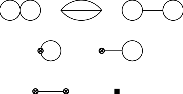
Figure 1: Skeleton diagrams of $O(p^{6})$. Normal vertices are from ${\cal L}_{p^{2}}$, crossed circles and the full square denote vertices from ${\cal L}_{p^{4}}$ and ${\cal L}_{p^{6}}$, respectively.

The coupling constants of the various Lagrangians in Table 1 absorb the divergences from loop diagrams leading to finite renormalized Green functions with scale dependent couplings, the so-called low-energy constants (LECs). As in all EFTs, the LECs parametrize the effect of “heavy” degrees of freedom that are not represented explicitly in the EFT Lagrangian. Determination of those LECs is a major task for CHPT. In addition to phenomenological information, further theoretical input is needed. Lattice gauge theory has already furnished values for some LECs. To bridge the gap between the low-energy domain of CHPT and the perturbative domain of QCD, large-$N_{c}$ motivated interpolations with meson resonance exchange have been used successfully to pin down some of the LECs.

Especially in cases where the knowledge of LECs is limited, renormalization group methods provide valuable information. As in renormalizable quantum field theories, the leading chiral logs $(\ln{M^{2}/\mu^{2}})^{L}$ with a typical meson mass $M$, renormalization scale $\mu$ and loop order $L$ can in principle be determined from one-loop diagrams only (Büchler and Colangelo, 2003). In contrast to the renormalizable situation, new derivative structures (and quark mass insertions) occur at each loop order preventing a straightforward resummation of chiral logs.

Among the many applications of CHPT in the meson sector are the determination of quark mass ratios and the analysis of pion-pion scattering where the chiral amplitude of NNLO has been combined with dispersion theory (Roy equations). Of increasing importance for precision physics (CKM matrix elements, $(g-2)_{\mu}$, …) are isospin violating corrections including radiative corrections where CHPT provides the only reliable approach in the low-energy region. Such corrections are also essential for the analysis of hadronic atoms like pionium, a $\pi^{+}\pi^{-}$ bound state.

CHPT has also been applied extensively in the single-baryon sector. There are several differences to the purely mesonic case. For instance, the chiral expansion proceeds more slowly and the nucleon mass $m_{N}$ provides a new scale that does not vanish in the chiral limit. The formulation of heavy baryon CHPT was modeled after HQET integrating out the nucleon modes of $O(m_{N})$. To improve the convergence of the chiral expansion in some regions of phase space, a manifestly Lorentz invariant formulation has been set up more recently (relativistic baryon CHPT). Many single-baryon processes have been calculated to N³LO in both approaches, e.g., pion-nucleon scattering. With similar methods as in the mesonic sector, hadronic atoms like pionic or kaonic hydrogen have been investigated.

5.2 Nuclear physics

In contrast to the meson and single-baryon sectors, amplitudes with two or more nucleons do not vanish in the chiral limit when the momenta of Goldstone mesons tend to zero. Consequently, the power counting is different in the many-nucleon sector. Multi-nucleon processes are treated with different EFTs depending on whether all momenta are smaller or larger than the pion mass.

In the very-low-energy regime $|\vec{p}|\ll M_{\pi}$, pions or other mesons do not appear as dynamical degrees of freedom. The resulting EFT is called “pionless EFT” and it describes systems like the deuteron where the typical nucleon momenta are $\sim\sqrt{m_{N}B_{d}}\simeq 45$ MeV ($B_{d}$ is the binding energy of the deuteron). The Lagrangian for the strong interactions between two nucleons has the form

$${\cal L}_{NN}=C_{0}\left(N^{\top}P_{i}N\right)^{\dagger}N^{\top}P_{i}N+\dots$$ (24)

where $P_{i}$ are spin-isospin projectors and higher-order terms contain derivatives of the nucleon fields. The existence of bound states implies that at least part of the EFT Lagrangian must be treated nonperturbatively. Pionless EFT is an extension of effective range theory that has long been used in nuclear physics. It has been applied successfully especially to the deuteron but also to more complicated few-nucleon systems like the $Nd$ and $n\alpha$ systems. For instance, precise results for $Nd$ scattering have been obtained with parameters fully determined from $NN$ scattering. Pionless EFT has also been applied to so-called halo nuclei where a tight cluster of nucleons (like ⁴He) is surrounded by one or more “halo” nucleons.

In the regime $|\vec{p}|>M_{\pi}$, the pion must be included as a dynamical degree of freedom. With some modifications in the power counting, the corresponding EFT is based on the approach of Weinberg (1990,1991) who applied the usual rules of the meson and single-nucleon sectors to the nucleon-nucleon potential (instead of the scattering amplitude). The potential is then to be inserted into a Schrödinger equation to calculate physical observables. The systematic power counting leads to a natural hierarchy of nuclear forces, with only two-nucleon forces appearing up to NLO. Three- and four-nucleon forces arise at NNLO and N³LO, respectively.

A lot of progress has been achieved in the phenomenology of few-nucleon systems. The two- and $n$-nucleon ($3\leq n\leq 6$) sectors have been pushed to N³LO and NNLO, respectively, with encouraging signs of “convergence”. Compton scattering off the deuteron, $\pi d$ scattering, nuclear parity violation, solar fusion and other processes have been investigated in the EFT approach. The quark mass dependence of the nucleon-nucleon interaction has also been studied.

Further reading

Appelquist, T. and Carazzone, J. (1975), Infrared singularities and massive fields, Phys. Rev. D11, 2856.
Beane, S.R. et al. (2000), From hadrons to nuclei: crossing the border, in Boris Ioffe Festschrift “At the frontier of particle physics”, Ed. M. Shifman and B. Ioffe, World Scientific (Singapore, 2001) [nucl-th/0008064].
Becher, T. (2004), B decays in the heavy-quark expansion, hep-ph/0411065.
Bedaque, P.F. and van Kolck, U. (2002), Effective field theory for few-nucleon systems, Ann. Rev. Nucl. Part. Sci. 52, 339 [nucl-th/0203055].
Bernard, V., Kaiser, N. and Meißner, U.-G. (1995), Chiral dynamics in nucleons and nuclei, Int. J. Mod. Phys. E4, 193 [hep-ph/9501384].
Bijnens, J. (2002), QCD and weak interactions of light quarks, in “At the frontier of particle physics”, Vol. 4, Ed. M. Shifman, World Scientific (Singapore, 2002) [hep-ph/0204068].
Bijnens, J. (2004), Chiral meson physics at two loops, hep-ph/0409068.
Brambilla, N., Pineda, A., Soto, J. and Vairo, A. (2004), Effective field theories for quarkonium, Rev. Mod. Phys. (in press), hep-ph/0410047.
Brambilla, N. et al. (Quarkonium Working Group) (2004), Heavy quarkonium physics, hep-ph/0412158.
Büchler, M. and Colangelo, G. (2003), Renormalization group equations for effective field theories, Eur. Phys. J. C32, 427 [hep-ph/0309049].
Buchmüller, W. and Wyler, D. (1986), Effective Lagrangian analysis of new interactions and flavour conservation, Nucl. Phys. B268, 621.
Colangelo, G., Gasser, J. and Leutwyler, H. (2001), $\pi\pi$ scattering, Nucl. Phys. B603, 125 [hep-ph/0103088].
D’Hoker, E. and Weinberg, S. (1994), General effective actions, Phys. Rev. D50, 6050 [hep-ph/9409402].
Ecker, G. (1995), Chiral perturbation theory, Prog. Part. Nucl. Phys. 35, 1 [hep-ph/9501357].
Ecker, G. (1998), Chiral symmetry, in Proc. of Schladming Winter School 1998: “Broken symmetries”, Eds. L. Mathelitsch and W. Plessas, Lecture Notes in Physics 521, Springer (Berlin, 1999) [hep-ph/9805500].
Ecker, G. (2000), Strong interactions of light flavours, in Proc. of Advanced School on Quantum Chromodynamics, Benasque, Spain, Eds. S. Peris and V. Vento, Univ. Autonoma de Barcelona (Barcelona, 2001) [hep-ph/0011026].
Feruglio, F. (1993), The chiral approach to the electroweak interactions, Int. J. Mod. Phys. A8, 4937 [hep-ph/9301281].
Fleming, S. (2003), The large energy expansion for B decays: soft collinear effective theory, in Proc. of “Flavour Physics and CP Violation”, Paris, Ed. P. Perret, Ecole Polytechnique (Palaiseau, 2003) [hep-ph/0309133].
Gasser, J. and Leutwyler, H. (1984), Chiral perturbation theory to one loop, Ann. Phys. 158, 142.
Gasser, J. and Leutwyler, H. (1985), Chiral perturbation theory: expansions in the mass of the strange quark, Nucl. Phys. B250, 465.
Gasser, J. (2003), Light quark dynamics, in Proc. of Schladming Winter School 2003: “Flavour physics”, Eds. U.-G. Meißner and W. Plessas, Lecture Notes in Physics 629, Springer (Berlin, 2004) [hep-ph/0312367].
Georgi, H. (1993), Effective field theory, Ann. Rev. Nucl. Part. Sci. 43, 209.
Hill, C. T. and Simmons, E. H. (2003), Strong dynamics and electroweak symmetry breaking, Phys. Rept. 381, 235, Err. ibid. 390, 553 (2004) [hep-ph/0203079].
Hinchliffe, I., Kersting, N. and Ma, Y.L. (2004), Review of the phenomenology of noncommutative geometry, Int. J. Mod. Phys. A19, 179 [hep/0205040].
Hoang, A.H. (2002), Heavy quarkonium dynamics, in “At the frontier of particle physics”, Vol. 4, Ed. M. Shifman, World Scientific (Singapore, 2002) [hep-ph/0204299].
Kaplan, D.B. (1995), Effective field theories, Lectures at 7th Summer School in Nuclear Physics, Seattle, Washington, nucl-th/9506035.
Leutwyler, H. (1994), On the foundations of chiral perturbation theory, Ann. Phys. 235, 165 [hep-ph/9311274].
Leutwyler, H. (2000), Chiral dynamics, in Boris Ioffe Festschrift: “At the frontier of particle physics”, Ed. M. Shifman and B. Ioffe, World Scientific (Singapore, 2001) [hep-ph/0008124].
Mannel, T. (2004), Effective field theories in flavour physics, Springer Tracts in Modern Physics 203, Springer (Berlin, 2004).
Manohar, A.V. (1996), Effective field theories, in Proc. of Schladming Winter School 1996: “Perturbative and nonperturbative aspects of quantum field theory”, Eds. H. Latal and W. Schweiger, Lecture Notes in Physics 479, Springer (Berlin, 1997) [hep-ph/9606222].
Manohar, A.V. and Wise, M.B. (2000), Heavy quark physics, Camb. Monogr. Part. Phys. Nucl. Phys. Cosmol. 10, 1.
Meißner, U.-G. (2005), Modern theory of nuclear forces, Nucl. Phys. A751, 149 [nucl-th/0409028].
Neubert, M. (2004), Theory of exclusive hadronic B decays, Lecture Notes in Physics 647, Springer (Berlin, 2004).
Pich, A. (1995), Chiral perturbation theory, Rept. Prog. Phys. 58, 563 [hep-ph/9502366].
Pich, A. (1998), Effective field theory, in Proc. of Les Houches Summer School 1997: “Probing the standard model of particle interactions”, Eds. R. Gupta et al., Elsevier (Amsterdam, 1999) [hep-ph/9806303].
Rafael, E. de (1995), Chiral Lagrangians and CP violation, in Proc. of TASI 1994: “CP violation and the limits of the Standard Model”, Ed. J. F. Donoghue, World Scientific (River Edge, 1995) [hep-ph/9502254].
Rothstein, I.Z. (2003), Effective field theories, in Proc. of TASI 2002: “Particle physics and cosmology: the quest for physics beyond the standard model”, Eds. H.E. Haber and A.E. Nelson, World Scientific (River Edge, 2004) [hep-ph/0308266].
Savage, M. (2003), Effective field theory for nuclear physics, nucl-th/0301058.
Scherer, S. (2002), Introduction to chiral perturbation theory, Adv. Nucl. Phys. 27, 277, Ed. J.W. Negele et al. [hep-ph/0210398].
Stewart, I.W. (2003), Theoretical introduction to B decays and the soft collinear effective theory, hep-ph/0308185.
Szabo, R.J. (2003), Quantum field theory in noncommutative spaces, Phys. Rept. 378, 207 [hep-th/0109162].
Weinberg, S. (1979), Phenomenological Lagrangians, Physica A96, 327.
Weinberg, S. (1990), Nuclear forces from chiral Lagrangians, Phys. Lett. B251, 288.
Weinberg, S. (1991), Effective chiral Lagrangians for nucleon-pion interactions and nuclear forces, Nucl. Phys. B363, 3.