Fractional momentum correlations in multiple production of W bosons and of ${b\bar{b}}$ pairs in high energy $pp$ collisions

Abstract

Multiple parton collisions will represent a rather common feature in $pp$ collisions at the LHC, where regimes with very large momentum transfer may be studied and events rare in lower energy accelerators might occur with a significant rate. A reason of interest in large $p_{t}$ regimes is that, differently from low $p_{t}$, evolution will induce correlations in $x$ in the multiparton structure functions. We have estimated the cross section of multiple production of $W$ bosons with equal sign, where the correlations in $x$ induced by evolution are particularly relevant, and the cross section of $b\bar{b}b\bar{b}$ production, where the effects of evolution are much smaller. Our result is that, in the case of multiple production of $W$ bosons, the terms with correlations may represent a correction of the order of 40% of the cross sections, for $pp$ collisions at 1 TeV c.m. energy, and a correction of the order of 20% at 14 TeV. In the case of $b\bar{b}$ pairs the correction terms are of the order of $10-15\%$ at 1 TeV and of the order of 5% at 14 TeV.

I Introduction

Multiple parton interactions in high energy hadronic collisions have been discussed long ago by several authors Landshoff ; Paver . Experimentally events with multiparton interactions have been first observed in $pp$ collisions by the AFS Collaboration Akesson:1986iv and later, with sizably larger statistics, at Fermilab by the CDF Collaboration CDF .

In multiple parton collisions the hadron is probed in different points contemporarily Paver . The non trivial feature of multiple parton collisions is hence its non-perturbative input, which has a direct relation with the correlations between partons in the hadron structure Calucci:1997ii . As the process is originated by the large population of partons in the initial state, the expectation is nevertheless that correlations should not represent a major feature in the process, with the exception of correlations in transverse space, which are directly measured by the cross section. Indeed the experimental analysis and most of the theoretical estimates have been done with this simplifying assumption and, although the statistics was too low to draw firm conclusions, the CDF Collaboration reported that the cross section is not influenced appreciably when changing the fractional momenta of initial state partons CDF .

The much larger rates of multiple parton collisions expected at the LHC, with the possibility of testing different multiparton processes at different resolution scales, represents however a good motivation for reconsidering the approach to the problem. In particular an interesting process, where multiple parton collisions play an important role and which might be observed at the LHC, is the production of multiple $W$ bosons with equal sign Stirling1 , which would allow testing multiple parton interactions at a much larger resolution scale than usually considered. The evolution of the multiparton structure functions will play a non minor role in this case, leading to sizable correlations in fractional momenta.

The purpose of the present note is to give some quantitative indication of the effects in multiparton collisions in a high resolution regime and compare with a case at a lower resolution. After recalling the basic features of the inclusive cross section of double parton collisions, we will hence evolve double parton distributions at high resolution scales. The effect of correlations induced by evolution will be estimated studying the cross sections of multiple production of equal sign $W$ bosons and the cross section of multiple production of $b\bar{b}$ pairs, in the energy range $1-14$ TeV.

II Double parton cross section

With the only assumption of factorization of the two hard parton processes A and B, the inclusive cross section of a double parton-scattering process in a hadronic collision is expressed by Paver ; Braun

$$\sigma^{D}_{(A,B)}=\frac{m}{2}\sum_{i,j,k,l}\int\Gamma_{ij}(x_{1},x_{2},b)\,\hat{\sigma}^{A}_{ik}(x_{1},x_{1}^{\prime})\,\hat{\sigma}^{B}_{jl}(x_{2},x_{2}^{\prime})\,\Gamma_{kl}(x_{1}^{\prime},x_{2}^{\prime};b)\,dx_{1}\,dx_{1}^{\prime}\,dx_{2}\,dx_{2}^{\prime}\,d^{2}b,$$ (1)

where $\Gamma_{ij}(x_{1},x_{2},b)$ are the double parton distribution functions, depending on the fractional momenta $x_{1},\,x_{2}$ and on the relative transverse distance $b$ of the two partons undergoing the hard processes A and B, the indices $i$ and $j$ refer to the different parton species and $\hat{\sigma}^{A}_{ik}$ and $\hat{\sigma}^{B}_{jl}$ are the partonic cross sections. The dependence on the resolution scales is implicit in all quantities. The factor $m/2$ is a consequence of the symmetry of the expression for interchanging $i$ and $j$; specifically $m=1$ for indistinguishable parton processes and $m=2$ for distinguishable parton processes.

The double distributions $\Gamma_{ij}(x_{1},x_{2},b)$ are the main reason of interest in multiparton collisions. The distributions $\Gamma_{ij}(x_{1},x_{2},b)$ contain in fact all the information of probing the hadron in two different points contemporarily, though the hard processes A and B.

The cross section for multiparton process is sizable when the flux of partons is large, namely at small $x$, and dies out quickly for larger values. Given the large parton flux one may hence expect that correlations in momentum fraction will not be a major effect and partons to be rather correlated in transverse space (as they must anyhow all belong to the same hadron). Neglecting the effect of parton correlations in $x$ one writes

$$\Gamma_{ij}(x_{1},x_{2};b)=\Gamma_{i}(x_{1})\,\Gamma_{j}(x_{2})\,F^{i}_{j}(b),$$ (2)

where $\Gamma_{i}(x)$ are the usual one body parton distribution function and $F^{i}_{j}(b)$ is a function normalized to one and representing the parton pair density in transverse space. The inclusive cross section hence simplifies to

$$\sigma^{D}_{(A,B)}=\frac{m}{2}\sum_{ijkl}\Theta^{ij}_{kl}\,\hat{\sigma}_{ij}(A)\,\hat{\sigma}_{kl}(B),$$ (3)

where $\hat{\sigma}_{ij}(A)$ and $\hat{\sigma}_{kl}(B)$ are the hadronic inclusive cross sections for the two partons labelled $i$ and $j$ to undergo the hard interaction labelled $A$ and for two partons $k$ and $l$ to undergo the hard interaction labelled $B$;

$$\Theta^{ij}_{kl}=\int d^{2}b\,F^{i}_{k}(b)\,F^{j}_{l}(b)$$ (4)

are geometrical coefficients with dimension an inverse cross section and depending on the various parton processes. In the simplified scheme above, the coefficients $\Theta^{ij}_{kl}$ are the experimentally accessible quantities carrying the information of the parton correlations in transverse space.

In the experimental search of multiple parton collisions the cross section has been further simplified assuming that the densities $F^{i}_{j}$ do not depend on the indices $i$ and $j$, which leads to the expression

$$\sigma^{D}_{(A,B)}=\frac{m}{2}\,\frac{\hat{\sigma}(A)\,\hat{\sigma}(B)}{\sigma_{eff}}\equiv\sigma_{fact}^{D},$$ (5)

where all information on the structure of the hadron in transverse space is summarized in the value of a single the scale factor, $\sigma_{eff}$. In the experimental study of double parton collisions CDF quotes $\sigma_{eff}=14.5\,mb$ CDF .

The experimental evidence is not inconsistent with the simplest hypothesis of neglecting correlations in momentum fractions, the resolution scale probed in the CDF experiment is however not very large, the transverse momenta of final state partons being of the order of 5 GeV. We will hence approach the problem in more general terms, focusing on multiple production of equal sign $W$ bosons and of $b\bar{b}b\bar{b}$ pairs, keeping into account the correlations in fractional momenta induced by evolution.

III Two-body distribution functions

The evolution of the double parton distribution function has been discussed in refs Kirschner ; Shelest and more recently in Snigirev . The approach is essentially the same used to study particle correlations in the fragmentation functions Puhala , using the jet calculus rules Konishi .

Introducing the dimensionless variable

$$t=\frac{1}{2\,\pi\,b}\ln\left[1+\frac{g^{2}(\mu^{2})}{4\,\pi}b\,\ln\left(\frac{Q^{2}}{\mu^{2}}\right)\right],\,\,\,b=\frac{33-2\,n_{f}}{12\,\pi},$$

where $g^{2}(\mu^{2})$ is the running coupling constant at the reference scale $\mu^{2}$ and $n_{f}$ the number of active flavors, the probability $D_{h}^{j_{1}j_{2}}(x_{1},x_{2};t)$ to find two partons of types $j_{1}$ and $j_{2}$ with fractional momenta $x_{1}$ and $x_{2}$ satisfy the generalized Lipatov-Altarelli-Parisi-Dokshitzer evolution equation

$$\frac{dD_{h}^{j_{1}j_{2}}(x_{1},x_{2};t)}{dt} =\sum_{j_{1}^{\prime}}\int_{x_{1}}^{1-x_{2}}\,\frac{dx_{1}^{\prime}}{x_{1}^{\prime}}\,D_{h}^{j_{1}^{\prime}j_{2}}(x_{1}^{\prime},x_{2};t)\,P_{j_{1}^{\prime}\to j_{1}}\left(\frac{x_{1}}{x_{1}^{\prime}}\right)$$

$$+\sum_{j_{2}^{\prime}}\int_{x_{2}}^{1-x_{1}}\,\frac{dx_{2}^{\prime}}{x_{2}^{\prime}}\,D_{h}^{j_{1}j_{2}^{\prime}}(x_{1},x_{2}^{\prime};t)\,P_{j_{2}^{\prime}\to j_{2}}\left(\frac{x_{2}}{x_{2}^{\prime}}\right)$$

$$+\sum_{j^{\prime}}D_{h}^{j^{\prime}}(x_{1}+x_{2};t)\frac{1}{x_{1}+x_{2}}\,P_{j^{\prime}\to j_{1}j_{2}}\left(\frac{x_{1}}{x_{1}+x_{2}}\right),$$ (6)

where the subtraction terms are included in the evolution kernels $P$.

If at the scale $\mu^{2}$ one assumes the factorized form

$$D_{h}^{j_{1}j_{2}}(z_{1},z_{2},0)=D_{h}^{j_{1}}(z_{1};0)\,D_{h}^{j_{2}}(z_{2};0)\,\theta(1-z_{1}-z_{2}),$$ (7)

at a larger scale one obtains a solution which may be expressed as the sum of a factorized and of two non-factorized contributions:

$$D_{h}^{j_{1}j_{2}}(x_{1},x_{2};t)=D_{h}^{j_{1}}(x_{1};t)\,D_{h}^{j_{2}}(x_{2};t)\,\theta(1-x_{1}-x_{2})+D_{h,corr,1}^{j_{1}j_{2}}(x_{1},x_{2};t)+D_{h,corr,2}^{j_{1}j_{2}}(x_{1},x_{2};t),$$ (8)

where the non-factorized contributions are expressed by the convolutions:

$$D_{h,corr,1}^{j_{1}j_{2}}(x_{1},x_{2};t) =\theta(1-x_{1}-x_{2})\,\left[\sum_{j_{1}^{\prime}j_{2}^{\prime}}\int_{x_{1}}^{1}\frac{dz_{1}}{z_{1}}\int_{x_{2}}^{1}\frac{dz_{2}}{z_{2}}\,D_{h}^{j_{1}^{\prime}}(z_{1},0)\,D_{j_{1}^{\prime}}^{j_{1}}(\frac{x_{1}}{z_{1}};t)\right.$$

$$\times\left.D_{h}^{j_{2}^{\prime}}(z_{2},0)\,D_{j_{2}^{\prime}}^{j_{2}}(\frac{x_{2}}{z_{2}};t)\,\,[\theta(1-z_{1}-z_{2})-1]\right]$$ (9)

$$D_{h,corr,2}^{j_{1}j_{2}}(x_{1},x_{2};t) =\sum_{j^{\prime}j_{1}^{\prime}j_{2}^{\prime}}\int_{0}^{t}dt^{\prime}\int_{x_{1}}^{1}\frac{dz_{1}}{z_{1}}\int_{x_{2}}^{1-x_{1}}\frac{dz_{2}}{z_{2}}\,D_{h}^{j^{\prime}}(z_{1}+z_{2};t^{\prime})\frac{1}{z_{1}+z_{2}}$$

$$\times\,P_{j^{\prime}\to j_{1}^{\prime}j_{2}^{\prime}}\left(\frac{z_{1}}{z_{1}+z_{2}}\right)\,D_{j_{1}^{\prime}}^{j_{1}}(\frac{x_{1}}{z_{1}};t-t^{\prime})\,D_{j_{2}^{\prime}}^{j_{2}}(\frac{x_{2}}{z_{2}};t-t^{\prime});$$ (10)

and the distribution functions $D_{i}^{j}(x;t)$ satisfy the evolution equation

$$\frac{dD_{i}^{j}(x;t)}{dt}=\sum_{j^{\prime}}\int_{x}^{1}\frac{dx^{\prime}}{x^{\prime}}D_{i}^{j^{\prime}}(x^{\prime};t)\,P_{j^{\prime}-j}\left(\frac{x}{x^{\prime}}\right).$$ (11)

with initial condition $D_{i}^{j}(x;t=0)=\delta_{ij}\,\delta(1-x)$

Equations(11) are solved by introducing the Mellin transforms

$$D_{i}^{j}(n;t)=\int_{0}^{1}dx\,x^{n}\,D_{i}^{j}(x;t),$$ (12)

which lead to a system of ordinary linear-differential equations at the first order. The solution is given by the inverse Mellin transform

$$D_{i}^{j}(x;t) = \int\frac{dn}{2\,\pi\,\imath}x^{-n}\,D_{i}^{j}(n;t)=\mathcal{L}^{-1}(D_{i}^{j}(n;t),-\ln(x)),$$ (13)

where the integration runs along the imaginary axis at the right of all the $n$ singularities, while $\mathcal{L}^{-1}$ represents the Inverse Laplace operator.

The double distributions can then be obtained numerically. For inverting the Laplace Transform we have followed two different procedures Abate : the Gaver-Wynn-Rho (GWR) algorithm and the fixed Talbot (FT) method. The first procedure (GWR) is based on a special acceleration sequence of the Gaver functionals and requires to evaluate the transform only on the real axes; the second procedure (FT) is based on the deformation of the contour of the Bromwich inversion integral and requires complex arithmetic. Comparing the two methods we have found more stable results when using the (FT) method. The double distributions have hence been obtained by numerical integration with the Vegas algorithm Vegas , using the MRS99 MRS99 as input parton distribution function at the scale $\mu^{2}$.

In the kinematical range of interest for the actual case (we never exceed $x=.1$) the contribution of the term $D_{h,corr,1}^{j_{1}j_{2}}$ in eq.(8) is negligible. The first term in eq.(8) represents the factorized contribution usually considered and is the solution of the homogeneous (LAPD) evolution equation, while the third term is a particular solution of the complete equation.

The effect of the correlation terms induced by evolution is shown for gluon-gluon and for quark-quark in Fig.[1,2], where the ratio

$$R^{j_{1}j_{2}}(x_{1},x_{2};t)=\frac{D_{h,corr,1}^{j_{1}j_{2}}(x_{1},x_{2};t)+D_{h,corr,2}^{j_{1}j_{2}}(x_{1},x_{2};t)}{D_{h}^{j_{1}}(x_{1};t)\,D_{h}^{j_{2}}(x_{2};t)}.$$ (14)

is plotted as a function of $x$, with $x_{1}=x_{2}=x$, with the following choice of parameters: $\mu=1.2\,GeV$, $n_{f}=4$, factorization scale equal to the $W$ mass, $m_{w}=80.4\,GeV$ (solid curves) and factorization scale equal to the bottom quark mass, $m_{b}=4.6\,GeV$ (dashed curves).

As shown in Fig.[1], the ratio $R^{gg}$ is nearly $35\%$ for $x\sim 0.1$ and decreases up to $8-10\%$ for $x\sim 0.01$ and to $2\%$ for $x\sim 0.001$, when the $W$ mass is used as factorization scale. When taking the $b$ quark mass as factorization scale, the value of the ratio is of the order of $10-12\%$ for $x\sim 0.1$ and decreases up to $5\%$ and to $2\%$ for $x\sim 0.01$ and $x\sim 0.001$ respectively. The ratio would of course be much larger (up to $60\%$) if going to larger $x$ values.

The ratio $R^{qq}$ is shown in Fig.[2] for a few flavor choices. With the $W$ mass as factorization scale, the ratios are of the order of $35,\,20,\,10\%$ for $x\sim 0.1,\,0.01,\,0.001$. With the $b$ quark mass as factorization scale the ratios are of order of $23,\,10,\,5\%$ for $x\sim 0.1,\,0.01,\,0.001$.
Apart from the case of hadron-nucleus collisions, when two different target nucleons take part to the process Strikman:2001gz , the non-perturbative input of the double parton scattering cross section is not represented however by the distribution functions $D^{j_{1}j_{2}}_{h}(x_{1},x_{2};t)$ in Eq.(8), where all transverse variables have been integrated. The double parton scattering cross section, Eq.(1), depends in fact in a direct way also on the relative separation of partons in transverse space, which is of the order of the hadron size and hence outside the control of perturbation theory.

Considering that the longitudinal and the transverse momenta of initial state partons are essentially decoupled in the process, because of the different scales involved, it’s not unreasonable to assume phenomenologically a factorized dependence of the double distribution functions on the longitudinal and transverse degrees of freedom. Given the different origin of the terms in $D_{h}^{j_{1}j_{2}}$, it’s also not unnatural to consider the possibility of having different non-perturbative scales, for the transverse separation of the factorized and of the correlated terms. In fact, although in the general case evolution would mix the two scales in the $D_{h,corr,1}^{j_{1}j_{2}}$ term, the term $D_{h,corr,1}^{j_{1}j_{2}}$ is very small in the kinematical regime of interest and the hypothesis of two different transverse scales is not inconsistent.

We hence assume that the typical transverse distance between partons in $D_{h,fact}^{j_{1}j_{2}}$ and in $D_{h,corr,1}^{j_{1}j_{2}}$ corresponds to the relatively low resolution scale process observed by CDF and, to have an idea on the effects of the presence of two different scales in the double parton densities, we introduce a different transverse distance in the term $D_{h,corr,2}^{j_{1}j_{2}}$, related to the size of the gluon cloud of a valence quark, and corresponding to a relatively shorter range correlation term. The double parton distributions are hence expressed in the following way:

$$D_{h}^{j_{1}j_{2}}(x_{1},x_{2};b;t)=\left(D_{h,fact}^{j_{1}j_{2}}(x_{1},x_{2};t)+D_{h,corr,1}^{j_{1}j_{2}}(x_{1},x_{2};t)\right)\,F_{\sigma_{eff}}(b)+D_{h,corr,2}^{j_{1}j_{2}}(x_{1},x_{2};t)\,F_{\sigma_{r}}(b)$$

where the parton pair densities $F_{i}(b)$ satisfy

$$\int d^{2}b\,F_{i}(b)=1\quad\int d^{2}b\,F_{i}(b)^{2}=\frac{1}{\sigma_{i}}$$

with $i=\sigma_{eff},\,\sigma_{r}$.

While $F_{\sigma_{eff}}$ represents the transverse density of partons at a relatively low resolution scale, relevant in the kinematical conditions of the CDF experiment and leading to the measured value of the scale factor $\sigma_{eff}=14.5$ mb, $F_{\sigma_{r}}$ is rather the transverse parton density characterizing partons correlated in fractional momentum, which becomes increasingly important when the resolution scale is large. To study the effect of the two scales we have let the smaller scale vary in the interval $\sigma_{r_{0}}\leftrightarrow\sigma_{eff}$ assuming $\sigma_{r_{0}}=2.8$ mb Povh , which might represent the size of the gluon cloud of a valence quark in the hadron. To disentangle the effects of the correlation in fractional momenta we have neglected a possible dependence of the parton pair densities $F_{i}(b)$ on the partons flavor.

IV Multiple production of $b\bar{b}$ pairs and of equal sign $W$ bosons in $pp$ collisions

For the purpose of the present analysis we have hence evaluated the contributions to multiple production of equal sign $W$ bosons and to multiple production of $b\bar{b}$ pairs, due to multiple (disconnected) parton collision processes, taking into account the correlation terms in fractional momenta induced by evolution.

As a matter of fact higher order corrections in $\alpha_{S}$ are very important in heavy quark production. To the purpose of the present analysis we have evaluated the cross section at the lowest order in perturbation theory, taking higher order corrections into account by rescaling the lowest order results with a constant factor $K$, defined as the ratio between the inclusive cross-section for $b\bar{b}$ production, $\sigma(b\bar{b})$, and the result of the lowest-order calculation in pQCD. Our assumption is hence that higher order corrections in $b\bar{b}b\bar{b}$ production may be taken into account by multiplying the cross section of each connected process by the same factor $K$, so that higher order corrections are taken into account by multiplying the lowest order cross section by the $K$-factor at the second power. In the actual calculation we have used a $K$ factor equal to $5.7$ (Cattaruzza ; DelFabbro4 ) and the value $m_{b}=4.6\,GeV$ for the mass of the bottom quark.

The multiparton distributions have been obtained, as described in the previous paragraph, using as input distributions at the scale $\mu^{2}$ the MRS99 MRS99 parton distribution functions. Factorization and renormalization scale have been set equal to the transverse mass of the produced quarks. As for the dependence on the transverse variables, in addition to the usual factorized contribution, leading to the scale factor $1/\sigma_{eff}$, in the present case the cross section includes also non factorized contributions, corresponding to the couplings of $D_{h,corr,2}^{ik}$ both with $D_{h,fact,1}^{jl}$ and with $D_{h,corr,2}^{ik}$. We have assumed a gaussian distribution for $F_{\sigma_{eff}}(b)$ and for $F_{\sigma_{r}}(b)$. The scale factors are correspondingly $2/(\sigma_{eff}+\sigma_{r})$ and $1/\sigma_{r}$.

In Fig.[1] we plot the $gg$ correlation (the dominant contribution to $b\bar{b}$ is gluon fusion) while the expected rise of the total $b\bar{b}b\bar{b}$ cross-section is plotted in Fig.[3] (left-panel) as a function of the center of mass energy. The dashed curve refers to the double-parton scattering factorized term ($\sigma_{fact}^{D}$) given by eq.(5); the continuous curves refer to the double-parton scattering correlation contributions ($\sigma_{corr}^{D}$), with geometrical factors determined by setting $r=r_{0}$ (upper curve) and $r=r_{eff}$ (lower curve). The ratio between the contribution of the terms with correlations and the factorized term is shown in Fig.[3] (right panel) as a function of center of mass energy. The effect of the terms with correlations decreases by increasing the center of mass energy; depending on the values of $r\in[r_{eff},r_{0}]$, correction effects may vary between $(12-20)\%$ at $\sqrt{s}=1\,TeV$ and $(3.5-6)\%$ at $\sqrt{s}=14\,TeV$. The decrease is faster as $\sqrt{s}\leq 5\,TeV$: for larger c.m. energies the average fractional momentum $<x>$ becomes smaller than $0.01$, where the fraction $R^{gg}$ stabilizes around $0.03-0.05$, consistently with the amount of correction obtained for $\sqrt{s}>5\,TeV$.

In Fig.[4] we plot the $b\bar{b}b\bar{b}$ production cross-section at $\sqrt{s}=14\,TeV$ (left-panel) and at $\sqrt{s}=5.5\,TeV$ (right-panel), as a function of the minimum value of transverse momenta of the outgoing $b$ quarks $p_{t}^{min}$, in the pseudorapidity interval $|\eta|<0.9$. At $\sqrt{s}=14\,TeV$ with $p_{t}^{min}\in[0,10]\,GeV$ one has $<x>\in[1.2,3.4]\times 10^{-3}$, which leads to a contribution of the correlation terms of the order of $(2-4)\%$ and of $(4-7)\%$, respectively for the lower and the higher choices of $p_{t}^{min}$ Fig.(5)(left-panel). At $\sqrt{s}=5.5\,TeV$, in the considered range of variability of $p_{t}^{min}$ one has $<x>\in[3.5,6.5]\times 10^{-3}$ and the contribution of the correlation terms can become of the order of $12\%$, Fig.(5)(right-panel).

The cross sections of like-sign W pair production are evaluated at the leading order, hence including only quark initiated processes in the elementary interaction ($q\bar{q}^{\prime}\to W$). Higher order corrections are taken into account multiplying the lowest order cross section by the factor $K\simeq 1+(8\,\pi/9)\,\alpha_{s}(M_{W}^{2})$ Barger . We plot in fig.[6] (left-panel) the $W^{+}W^{+}$ cross-section as a function of the $pp$ center of mass energy. As in the case of $b\bar{b}b\bar{b}$ production, the dashed curve refers to the double-parton scattering factorized term ($\sigma_{fact}^{D}$), while the solid curves to the contribution of the terms with correlations ($\sigma_{corr}^{D}$), for the two different choices $r=r_{0}$ and $r=r_{eff}$. As one may infer from the behavior of the qq-correlation ratio, for $<x>\in[0.2,\,6]\times 10^{-2}$, which corresponds to the energy interval considered, the corrections due to the correlation terms range from $(27-45)\%$ at $\sqrt{s}=1\,TeV$ to $(7.5-13)\%$ at $\sqrt{s}=14\,TeV$, depending on the choice of $\sigma_{r}$. The results for $W^{-}W^{-}$ production are presented in fig.(7). As shown in the right panel the correlation terms can give contributions ranging from $(23-40)\%$ at $1\,TeV$ to $(12-20)\%$ at $14\,TeV.$

V Conclusions

As an effect of evolution, the multiparton distributions functions are expected to become strongly correlated in momentum fraction at large $Q^{2}$ and finite $x$ Kirschner ; Shelest ; Snigirev . On the other hand, the indications from the experimental observation of multiparton collisions at Fermilab CDF are not in favor of strong correlation effects in fractional momenta. The most likely reason being that the kinematical domain observed, relatively low $x$ values and limited resolution scale, is far from the limiting case considered in QCD.

The possibility of testing multiparton collisions at high resolution scales at the LHC will open the opportunity of testing the correlations predicted by evolution. To have an indication on the importance of the effects to be expected, we have considered a high resolution scale multiparton process (equal sign $W$ pair production) and, for comparison, a sizably smaller resolution scale process ($b\bar{b}b\bar{b}$ production) in $pp$ collisions in the energy range $1{\rm TeV}\leq\sqrt{s}\leq 14{\rm Tev}$. In both cases the production process may take place either by single (connected) or by multiple (disconnected) hard parton collisions, while the two contributions may be disentangled applying proper cuts in the final state CDF ; Stirling1 ; DelFabbro4 . To study the effects of correlations we have hence worked out the disconnected contributions to the cross sections after evolving the multiparton distribution functions at high resolution scales.

Our result is that the contribution of the terms with correlations, in equal sign $W$ pairs production, might be almost 40% of the cross section at 1 TeV and might still be a 20% effect at the LHC. The effect is much smaller in $b\bar{b}b\bar{b}$ production, where corrections to the usually considered factorized distribution are typically between 5 and 10%.

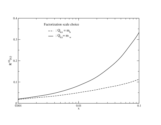
Figure 1: $gg$ correlation ratio for $x_{1}=x_{2}=x$, with factorization scale equal to the $W$ mass (solid- curve) and to the $b$ mass (dashed-curve).

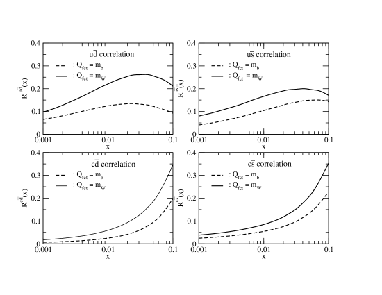
Figure 2: $qq$ correlation ratios for $x_{1}=x_{2}=x$, with factorization scale equal to the $W$ mass (solid- curves) and to the $b$ mass (dashed-curves).

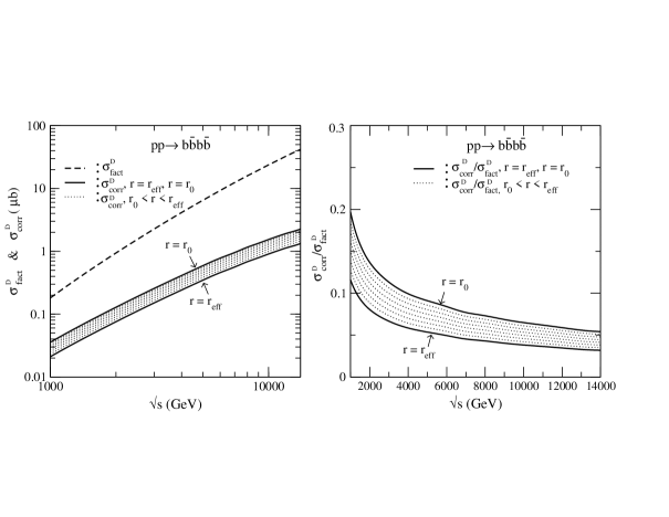
Figure 3: Left-panel: $b\bar{b}b\bar{b}$ inclusive cross-section as a function of center of mass energy; the dashed curve refers to the double-parton scattering factorized term $\sigma_{fact}^{D}$, while the upper and the lower solid curves refer to contributions with correlations $\sigma_{corr}^{D}$, with geometrical factors obtained setting $r=r_{0}$ and $r=r_{eff}$ respectively.
Right-panel: ratio between $\sigma_{corr}^{D}$ and $\sigma_{fact}^{D}$ as a function of center of mass energy.

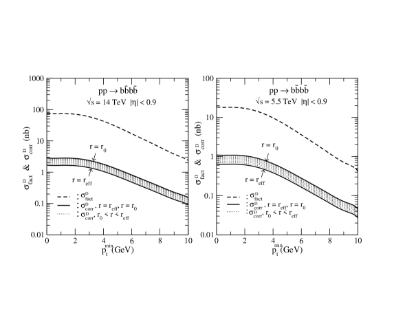
Figure 4: $b\bar{b}b\bar{b}$ production cross-section at $\sqrt{s}=14\,TeV$ and $\sqrt{s}=5.5\,TeV$ as a function of $p_{t}^{min}$, the minimum value of transverse momenta of the outgoing $b$ quarks; the dashed curves refer to the double-parton scattering factorized term $\sigma_{fact}^{D}$, while upper and lower solid curves refer to $\sigma_{corr}^{D}$ with geometrical factors obtained setting $r=r_{0}$ and $r=r_{eff}$ respectively.

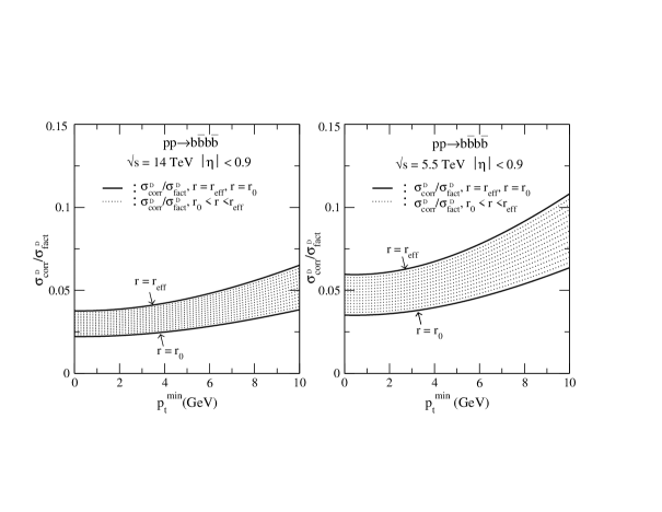
Figure 5: ratio between $\sigma_{corr}^{D}$ and $\sigma_{fact}^{D}$ at $\sqrt{s}=14\,TeV$ (left-panel) and $\sqrt{s}=5.5\,TeV$ (right-panel) as a function of $p_{t}^{min}$.

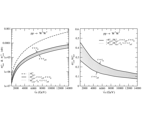
Figure 6: Left-panel: $W^{+}W^{+}$ inclusive cross-section as a function of the center of mass energy; the dashed curve refers to the double-parton scattering factorized term $\sigma_{fact}^{D}$, while upper and lower solid curves refer to $\sigma_{corr}^{D}$, with geometrical factors obtained setting $r=r_{0}$ and $r=r_{eff}$ respectively.
Right-panel: ratio between $\sigma_{corr}^{D}$ and $\sigma_{fact}^{D}$ as a function of center of mass energy.

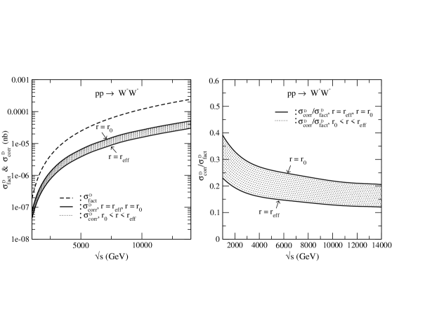
Figure 7: Left-panel: $W^{-}W^{-}$ inclusive cross-section as a function of the center of mass energy; the dashed curve refers to the double-parton scattering factorized term $\sigma_{fact}^{D}$, while the upper and the lower solid curves refer to the contribution with correlations $\sigma_{corr}^{D}$, with geometrical factors obtained setting $r=r_{0}$ and $r=r_{eff}$ respectively.
Right-panel: ratio between $\sigma_{corr}^{D}$ and $\sigma_{fact}^{D}$ as a function of center of mass energy.