Sum Rules for Magnetic Moments and Polarizabilities in QED and Chiral Effective-Field Theory

Abstract

We elaborate on a recently proposed extension of the Gerasimov-Drell-Hearn (GDH) sum rule which is achieved by taking derivatives with respect to the anomalous magnetic moment. The new sum rule features a linear relation between the anomalous magnetic moment and the dispersion integral over a cross-section quantity. We find some analogy of the linearized form of the GDH sum rule with the ‘sideways dispersion relations’. As an example, we apply the linear sum rule to reproduce the famous Schwinger’s correction to the magnetic moment in QED from a tree-level cross-section calculation and outline the procedure for computing the two-loop correction from a one-loop cross-section calculation. The polarizabilities of the electron in QED are considered as well by using the other forward-Compton-scattering sum rules. We also employ the sum rules to study the magnetic moment and polarizabilities of the nucleon in a relativistic chiral EFT framework. In particular we investigate the chiral extrapolation of these quantities.

I Introduction

The Gerasimov, Drell, Hearn (GDH) sum rule (SR) GDH , which relates a system’s anomalous magnetic moment to a weighted integral over a combination of doubly polarized photoabsorption cross sections, has received a good deal of attention in recent years. Impressive experimental programs to measure these photoabsorption cross-sections for the nucleon have recently been carried out at ELSA and MAMI (for a review see Ref. Drechsel:2004ki ). Such measurements provide an empirical test of the GDH SR, and can be used to generate phenomenological estimates of electromagnetic polarizabilities via related SRs, as will be discussed below. The GDH SR is particularly interesting because both its left- and right-hand-side can be reliably determined, thus providing a useful verification of the fundamental principles (such as unitarity and analyticity) which go into its derivation. At the present time the proton sum rule is satisfied within the experimental precision, while the case is still out for the neutron. However, it is not the purpose of this paper to discuss these experimental aspects of the SR, but rather to see what can be learned on the theoretical side.

Recently, we have shown Pascalutsa:2004ga that by taking derivatives of the GDH sum rule with respect to the anomalous magnetic moment one can obtain a new set of sum rule-like relations with intriguing properties. In particular, this procedure provided a sum rule involving the anomalous magnetic moment linearly rather than quadratically, which allows for the derivation of quantities such as the Schwinger moment in a much simpler fashion than via the usual GDH method. In this paper, we shall further examine these forms and apply them to the nucleon magnetic moment.

After a lightning review of the GDH and related sum rules (Sect. II), we derive the modified versions (Sect. III) and demonstrate that some of these relations have the form of so-called sideways dispersion relations (Sect. IV). Then we consider applications to the nucleon in the context of chiral perturbation theory and show how the new sum rules allow an elementary calculation (to one loop) of quantities such as magnetic moments (Sect. V) and polarizabilities (Sect. VI) to all orders in the heavy baryon expansion. The chiral behavior of the nucleon magnetic moments and polarizabilities is addressed in Sect. VII. Returning to QED in Sect. VIII, we demonstrate how the new sum rules can be applied to the two-loop calculation of the anomalous magnetic moment in a straightforward fashion. In the final section, we summarize our findings and suggest prospects for future work.

II Compton-scattering sum rules in QED

The forward-scattering amplitude describing the elastic scattering of a photon on a target with spin $s$ (real Compton scattering) is characterized by $2s+1$ scalar functions which depend on a single kinematic variable, e.g., the photon energy $\omega$. In the low-energy limit each of these functions corresponds to an electromagnetic moment—charge, magnetic dipole, electric quadrupole, etc.—of the target. In the case of a spin-1/2 target, the forward Compton amplitude is generally written as

$$T(\omega)={\vec{\varepsilon}\,^{\prime}}^{*}\cdot\vec{\varepsilon}\,f(\omega)+i\,\vec{\sigma}\cdot({\vec{\varepsilon}\,^{\prime}}^{*}\times\vec{\varepsilon})\,g(\omega)\,,$$ (1)

where $\vec{\varepsilon}$, $\vec{\varepsilon}\,^{\prime}$ is the polarization vector of the incident and scattered photon, respectively, while $\vec{\sigma}$ are the Pauli matrices representing the dependence on the target spin. The crossing symmetry of the Compton amplitude of Eq. (1) means invariance under $\varepsilon^{\prime}\leftrightarrow\varepsilon$, $\omega\leftrightarrow-\omega$, which obviously leads to $f(\omega)$ being an even and $g(\omega)$ being an odd function of the energy—$f(\omega)=f(-\omega)$, $g(\omega)=-g(-\omega)$. The two scalar functions $f(\omega),\,g(\omega)$ admit the following low-energy expansion,

$$f(\omega) = -\frac{e^{2}}{4\pi M}+(\alpha_{E}+\beta_{M})\,\omega^{2}+{\mathcal{O}}(\omega^{4})\ ,$$ (2a)

$$g(\omega) = -\frac{e^{2}\kappa^{2}}{8\pi M^{2}}\,\omega+\gamma_{0}\omega^{3}+{\mathcal{O}}(\omega^{5})\ ,$$ (2b)

and hence, in the low-energy limit, are given in terms of the target’s charge $e$ and anomalous magnetic moment (a.m.m.) $\kappa$. The next-to-leading order terms are given in terms of the nucleon electric ($\alpha_{E}$), magnetic ($\beta_{M}$), and forward spin ($\gamma_{0}$) polarizabilities.

In order to derive sum rules (SRs) for these quantities one assumes the scattering amplitude is an analytic function of $\omega$ everywhere but the real axis , which allows writing the real parts of the functions $f(\omega)$ and $g(\omega)$ as a dispersion integral involving their corresponding imaginary parts. The latter, on the other hand, can be related to combinations of doubly polarized photoabsorption cross-sections via the optical theorem,

$$\mbox{Im}\ f(\omega) = \frac{\omega}{8\pi}\left[\sigma_{1/2}(\omega)+\sigma_{3/2}(\omega)\right]\,,$$ (3a)

$$\mbox{Im}\ g(\omega) = \frac{\omega}{8\pi}\left[\sigma_{1/2}(\omega)-\sigma_{3/2}(\omega)\right]\,,$$ (3b)

where $\sigma_{\lambda}$ is the doubly-polarized total cross-section of the photoabsorption processes, with $\lambda$ specifying the total helicity of the initial system. Averaging over the polarization of initial particles gives the total unpolarized cross-section, $\sigma_{T}=\mbox{\small{$\frac{1}{2}$}}(\sigma_{1/2}+\sigma_{3/2})$.

After these steps one arrives at the results (see, e.g., Drechsel:2002ar for more details):

$$f(\omega) = f(0)\,+\,\frac{\omega^{2}}{2\pi^{2}}\,\int_{0}^{\infty}\frac{\sigma_{T}(\omega^{\prime})}{\omega^{\prime 2}-\omega^{2}-i\epsilon}\,d\omega^{\prime}\ ,$$ (4)

$$g(\omega) = -\frac{\omega}{4\pi^{2}}\,\int_{0}^{\infty}\frac{\Delta\sigma(\omega^{\prime})}{\omega^{\prime 2}-\omega^{2}-i\epsilon}\,\omega^{\prime}\,d\omega^{\prime}\ ,$$ (5)

with $\Delta\sigma\equiv\sigma_{3/2}-\sigma_{1/2}$, and where the sum rule for the unpolarized forward amplitude $f(\omega)$ has been once-subtracted to guarantee convergence. These relations can then be expanded in energy to obtain the SRs for the different static properties introduced in Eq. (2). In this way we obtain the Baldin SR Bal60 ; Lap63 :

$$\alpha_{E}+\beta_{M}=\frac{1}{2\pi^{2}}\,\int_{0}^{\infty}\,\frac{\sigma_{T}(\omega)}{\omega^{2}}\,d\omega\ ,$$ (6)

the GDH SR:

$$\frac{e^{2}\kappa^{2}}{2M^{2}}=\frac{1}{\pi}\int_{0}^{\infty}\,\frac{\Delta\sigma(\omega)}{\omega}\,d\omega\,,$$ (7)

a SR for the forward spin polarizability:

$$\gamma_{0}=\,-\,\frac{1}{4\pi^{2}}\,\int_{0}^{\infty}\,\frac{\Delta\sigma(\omega)}{\omega^{3}}\,d\omega\ .$$ (8)

and, in principle, one could continue in order to isolate higher order momentsmainz .

Let us now see how these sum rules are of use in field theory. We first consider the case of the electron in QED. To lowest order in the fine-structure constant, $\alpha_{em}=e^{2}/4\pi$, the photoabsorption process is given by the tree-level Compton scattering. The tree-level helicity amplitudes for this process are well known okla

$$\begin{array}[]{l}T(++;++)={-8\pi\alpha_{em}\over(M^{2}-s)^{2}(M^{2}-u)}((M^{2}-s)^{2}+M^{2}t)(M^{4}-su)^{1\over 2}\\ T(--;++)={-8\pi\alpha_{em}\over(M^{2}-s)^{2}(M^{2}-u)}(-M^{2}t)^{3\over 2},\\ T(-+;++)={8\pi\alpha_{em}\over(M^{2}-s)^{2}(M^{2}-u)}(M^{4}-su)(-M^{2}t)^{1\over 2},\\ T(++;+-)={8\pi\alpha_{em}\over(M^{2}-s)^{2}(M^{2}-u)}M^{2}t(M^{4}-su)^{1\over 2},\\ T(+-;+-)={-8\pi\alpha_{em}\over(M^{2}-s)^{2}(M^{2}-u)}(M^{4}-su)^{3\over 2},\\ T(-+;+-)={-8\pi\alpha_{em}\over(M^{2}-s)^{2}(M^{2}-u)}(-Ms)(-t)^{3\over 2},\end{array}$$ (9)

where $M$ is the electron mass; $s$, $t$ and $u$ are the Mandelstam variables. Using these results the unpolarized and double-polarized cross sections can be determined as:

$$\sigma_{T}^{(2)}(\omega) = {2\pi\alpha_{em}^{2}\over M^{2}}\left[{1+x\over x^{3}}\left({2x(1+x)\over 1+2x}-\log(1+2x)\right)\right.$$ (10)

$$+ \left.{1\over 2x}\log(1+2x)-{1+3x\over(1+2x)^{2}}\right]+{\cal O}(\alpha_{em}^{3}),$$

and

$$\Delta\sigma(\omega)=-{2\pi\alpha_{em}^{2}\over M^{2}x}\left[(1+{1\over x})\log(1+2x)-2\left(1+{x^{2}\over(1+2x)^{2}}\right)\right]+{\cal O}(\alpha_{em}^{3}),$$ (11)

where we have defined $x=\omega/M$. Substituting the latter expression into the r.h.s. of the GDH SR, Eq. (7), one can easily see that the integral vanishes exactly, which is required because otherwise the sum rule would lead to a nonsense result—the electron a.m.m. would receive contributions of order $\sqrt{\alpha_{em}}$.

At next order, ${\cal O}(\alpha_{em}^{3})$, the l.h.s. of the GDH SR receives a nonzero contribution in the form of the Schwinger correction: $\kappa=\alpha_{em}/2\pi$. In order to check that the same result is obtained on the r.h.s. of the sum rule is quite a formidable task since at this order one must know the Compton scattering amplitude to one loop, as well as account for the pair-production channel. Nevertheless, the calculation of the relevant helicity amplitudes was carried out more than three decades ago by Milton, Tsai, and deRaad and application to the GDH SR has relatively recently been performed by Dicus and Vega DiV01 , who verified (numerically) that the GDH SR holds at ${\cal O}(\alpha_{em}^{3})$ in QED.

Recently we have found a much simpler method by which to verify the GDH SR at this order. This technique is briefly described in the next section, while in the rest of the present section we examine the sum rules for polarizabilities, Eqs. (6) and (8). At first glance, such sum rules do not appear to be of much utility, since when evaluated in the case of QED, the static polarizabilities obtained therefrom diverge. However, this is not a problem, as pointed out by Llanta and Tarrach pol , who emphasized that one can determine well defined asymptotic forms in the limit as $\omega$ approaches zero. Thus, for example we can perform the integration for the spin even/odd amplitudes and determine that

$$f(\omega)-f(0)\simeq{\alpha_{em}^{2}\over\pi M}\left[{8\over 3}x^{2}\log 2x+{11x^{2}\over 18}+{266\over 15}x^{4}\log 2x+{1799\over 450}x^{4}+\ldots\right],$$ (12)

and

$$g(\omega)-g(0)\simeq{\alpha_{em}^{2}\over 2\pi M^{2}}\left[{20\over 3}x^{2}\log 2x+{37\over 9}x^{2}+{896\over 15}x^{4}\log 2x+{29\cdot 128\over 225}x^{4}+\ldots\right].$$ (13)

One can now use these expressions to define quasi-static polarizabilities, where by this we mean that these quantities contain both a constant term and a term which behaves as $\log\omega$—it is this latter piece that is responsible for the divergence as the static limit is taken. Thus, for example, we may define quasi-static values

$$\alpha_{E}^{q-s}+\beta_{M}^{q-s}={\alpha_{em}^{2}\over\pi M^{3}}\left[{8\over 3}\log 2x+{11\over 18}\right],$$ (14)

for the sum of electric and magnetic polarizabilities and

$$\gamma_{0}^{q-s}={\alpha_{em}^{2}\over 2\pi M^{4}}\left[{20\over 3}\log 2x+{37\over 9}\right],$$ (15)

for the forward spin polarizability. In this way we can also generate generalized sum rules for quadrupole and higher polarizabilities via Eqs. (4) and (5) mainz .

It is interesting to note that it is possible to determine the nonanalytic component of these quasi-static moments in a simpler fashion—by using only the the low energy expansion of the cross sections. That is, while the integrals

$$\int_{0}^{\Lambda}{dyy^{n}\over y^{2}-x^{2}},$$ (16)

are $\Lambda$-dependent if $n$ is an even integer, in the case that $n$ is odd there exists a $\Lambda$-independent logarithm

$$\int_{0}^{\Lambda}{dyy^{2\ell+1}\over y^{2}-x^{2}}=-x^{2\ell}\log x+...$$ (17)

which then determines the logarithmic component of the quasi-static polarizabilities. That is, since

$$\sigma_{tot}(\omega)={2\pi\alpha_{em}^{2}\over M^{2}}\left[{4\over 3}-{8\over 3}{\omega\over M}+{104\over 15}{\omega^{2}\over M^{2}}-{266\over 15}{\omega^{3}\over M^{3}}+\ldots\right],$$ (18)

and

$$\sigma_{3\over 2}(\omega)-\sigma_{1\over 2}(\omega)={2\pi\alpha_{em}^{2}\over M^{2}}\left[{4\over 3}{\omega\over M}-{20\over 3}{\omega^{2}\over M^{2}}+{108\over 5}{\omega^{3}\over M^{3}}+{896\over 15}{\omega^{4}\over M^{4}}+\ldots\right],$$ (19)

we require that the nonanalytic piece of the polarizabilities have the form

$$\alpha_{E}^{q-s}+\beta_{M}^{q-s}={\alpha_{em}^{2}\over\pi M^{2}}\left[{8\over 3}\log{\omega\over M}+...\right]$$

$$\gamma_{0}^{q-s}={\alpha_{em}^{2}\over 2\pi M^{4}}\left[{20\over 3}\log{\omega\over M}+\ldots\right],$$ (20)

in agreement with the exact forms given above. Likewise higher order forms can be determined.

We see then that the use of dispersive techniques in QED allows a straightforward extraction of information about polarizabilities and about the anomalous magnetic moment. As expected, the latter is complete agreement with the result obtained by conventional means, while the former requires such dispersive methods, since the corresponding static quantities are divergent.

III Derivatives of the GDH sum rule

We now review the derivation of the new form of sum rule. We begin by introducing a ‘classical’ (or ’trial’) value of the electron a.m.m., $\kappa_{0}$. At the Lagrangian level this amounts to the introduction of a Pauli term for the spin-1/2 field :

$${\cal L}_{\mbox{\small Pauli}}=\frac{i\kappa_{0}}{4M}\,\bar{\psi}\,\sigma_{\mu\nu}\,\psi\,F^{\mu\nu}\,,$$ (21)

where $F^{\mu\nu}$ is the electromagnetic field tensor and $\sigma_{\mu\nu}=(i/2)[\gamma_{\mu},\gamma_{\nu}]$ is the usual Dirac tensor operator. At the end of our calculation, we will set $\kappa_{0}$ to zero, but for now the total value of the a.m.m. is $\kappa=\kappa_{0}+\delta\kappa$, with $\delta\kappa$ denoting the loop contribution. (It is important to note that both $\delta\kappa$ and the cross-section become explicitly dependent on $\kappa_{0}$.) We then start taking derivatives of the GDH SR with respect to $\kappa_{0}$, which is subsequently set to zero, so that the total a.m.m. $\kappa$ returns to its usual loop value. We find

$$(4\pi^{2}\alpha_{em}/M^{2})\,\kappa\,\kappa^{\prime} = \int_{0}^{\infty}\!\Delta\sigma^{\prime}(\omega)\,\frac{d\omega}{\omega}\,,$$ (22)

$$(4\pi^{2}\alpha_{em}/M^{2})\,(\kappa^{\prime 2}+\kappa\,\kappa^{\prime\prime}) = \int_{0}^{\infty}\!\Delta\sigma^{\prime\prime}(\omega)\,\frac{d\omega}{\omega}\,,$$ (23)

and so on. To lowest order in $\alpha_{em}$ we find

$$(4\pi^{2}\alpha_{em}/M^{2})\,n\,\kappa^{(n-1)}=\int_{0}^{\infty}\!\!\Delta\sigma^{(n)}(\omega)\,\frac{d\omega}{\omega}\,,$$ (24)

where $\kappa^{(n)}$ denotes the $n$th derivative of $\kappa$ with respect to $\kappa_{0}$. This allows in principle the computation of $\kappa$ to order $\alpha_{em}^{n}$ by using the 1st to $n$th derivatives of the cross-section computed to order $\alpha_{em}^{n+1}$ to $\alpha_{em}^{2}$, respectively.

In particular, to lowest order we have the result :

$$\frac{4\pi^{2}\alpha_{em}}{M^{2}}\,\kappa=\int_{0}^{\infty}\!\left.\Delta\sigma^{\prime}(\omega)\right|_{\kappa_{0}=0}\,\frac{d\omega}{\omega}\,.$$ (25)

The striking feature of this sum rule is the linear relation between the a.m.m. and the (derivative of the) photoabsorption cross section, in contrast to the GDH SR where $\kappa$ appears quadratically, and although the cross-section quantity $\Delta\sigma^{\prime}(\omega)$ is not an observable, it is very clear how it can be determined within a specific theory. Thus, for example, the first derivative of the tree-level cross-section with respect to $\kappa_{0}$, at $\kappa_{0}=0$, in QED was worked out in Pascalutsa:2004ga :

$$\left.\Delta\sigma^{\prime}(\omega)\right|_{\kappa_{0}=0}=\frac{2\pi\alpha_{em}^{2}}{M\omega}\left[6-{2M\omega\over(M+2\omega)^{2}}-\left(2+{3M\over\omega}\right)\,\ln\left(1+\frac{2\omega}{M}\right)\right].$$ (26)

It is not difficult to find then that

$$\frac{1}{\pi}\int\limits_{0}^{\infty}\!\left.\Delta\sigma^{\prime}(\omega)\right|_{\kappa_{0}=0}\,\frac{d\omega}{\omega}=\frac{2\alpha_{em}^{2}}{M^{2}}\,.$$ (27)

Substituting this result in the linearized GDH SR, Eq. (25), we obtain $\kappa=\alpha_{em}/2\pi$—Schwinger’s one-loop result. We emphasize that this result is reproduced here by computing only a (derivative of the) tree-level Compton scattering cross-section and then performing an integration over energy. This is definitely much simpler than obtaining the Schwinger result from the GDH SR directly DiV01 , which requires input at the one-loop level. Along these lines, however, one can facilitate the two- and more loop calculations. We elaborate on this possibility in Sect. VIII.

IV Connection to sideways dispersion relations

It is interesting to observe that, by changing the integration variable to $s=M^{2}+2M\omega$, the linearized GDH SR, Eq. (25), can be written as

$$\kappa=\frac{M^{2}}{4\pi^{2}\alpha_{em}}\,\int\limits_{M^{2}}^{\infty}\!ds\,\frac{\left.\Delta\sigma^{\prime}(s)\right|_{\kappa_{0}=0}}{s-M^{2}}\,,$$ (28)

which is a special case of a ‘sideways dispersion relation’ as is demonstrated below.

The sideways dispersion for the a.m.m. is obtained by considering the half-off-shell electromagnetic vertex:

$$\Gamma^{\mu}(p^{\prime},p) = {\Lambda}^{(+)}(p/\,^{\prime})\left[F^{(+)}(s^{\prime},q^{2})\,\gamma^{\mu}+G^{(+)}(s^{\prime},q^{2})\,\frac{(p+p^{\prime})^{\mu}}{2M}\right]$$ (29)

$$+ {\Lambda}^{(-)}(p/\,^{\prime})\left[F^{(-)}(s^{\prime},q^{2})\,\gamma^{\mu}+G^{(-)}(s^{\prime},q^{2})\,\frac{(p+p^{\prime})^{\mu}}{2M}\right]\,,$$

with $q=p^{\prime}-p$ the photon momentum, $p^{\prime}$ the off-shell particle momentum ($s^{\prime}={p^{\prime}}^{2}$), and $p$ the on-shell momentum ($p^{2}=M^{2}$). Furthermore,

$${\Lambda}^{(\pm)}(p/)=\frac{p/\pm M}{2M}\,,$$ (30)

are the positive- and negative-energy state projections, and $F^{(\pm)}$ and $G^{(\pm)}$ are corresponding half-off-shell form factors. In this decomposition of the vertex, the a.m.m. is identified as $\kappa=-G^{(+)}(M^{2},0)$.

Akin to the Compton amplitudes considered above, the form factors must be analytic functions of $s^{\prime}$ everywhere in the complex plane except along the unitarity cut, which lies on the real axis for Re$\,s^{\prime}>M^{2}$. This analyticity allows a dispersive representation for each of the form factors:

$$F^{(\pm)}(s^{\prime},q^{2}) = \frac{1}{\pi}\int\limits_{M^{2}}^{\infty}ds\,\frac{{\rm Im}\,F^{(\pm)}(s,q^{2})}{s-s^{\prime}-i\epsilon}\,,$$ (31)

$$G^{(\pm)}(s^{\prime},q^{2}) = \frac{1}{\pi}\int\limits_{M^{2}}^{\infty}ds\,\frac{{\rm Im}\,G^{(\pm)}(s,q^{2})}{s-s^{\prime}-i\epsilon}\,,$$ (32)

and these relations are called sideways dispersion relations bincer60 ; drell65 .

In particular, from the relation for $G^{(+)}$ we find

$$\kappa=-\frac{1}{\pi}\int\limits_{M^{2}}^{\infty}ds\,\frac{{\rm Im}\,G^{(+)}(s,0)}{s-M^{2}}\,,$$ (33)

which is of the same form as the linearized GDH sum rule, Eq. (28). Specifically, one can show that

$${\rm Im}\,G^{(+)}(s,0)=-\frac{M^{2}}{e^{2}}\,\left.\Delta\sigma^{\prime}(s)\right|_{\kappa_{0}=0}+\frac{M^{2}}{e^{2}}\,\left[\Delta\sigma^{\prime}(s)-\Delta\sigma_{s}^{\prime}(s)\right]_{\kappa_{0}=0}\,,$$ (34)

where the second term integrates to 0. The function $\Delta\sigma_{s}^{\prime}$ is defined as the interference of the tree-level amplitude, Fig. 1, and the $s$-channel graphs with a Pauli-coupling insertion (first two graphs in Fig. 2). Recall that the function $\Delta\sigma^{\prime}$ is the interference of the tree-level graphs and both the $s$- and $u$-channel graphs with a Pauli-coupling insertion (the four graphs in Fig. 2), and analogous relations for the nucleon case will be discussed in the next section.

V Sum rules in chiral perturbation theory

Consider now a theory of nucleons interacting with pions via pseudovector coupling:

$${\cal L}_{\pi NN}=\frac{g}{2M}\,\bar{\psi}\,\gamma^{\mu}\,\gamma^{5}\,\tau^{a}\,\psi\,\partial_{\mu}\pi^{a},$$ (35)

where $g$ is the pion-nucleon coupling constant, $M$ is the nucleon mass, $\tau^{a}$ are isospin Pauli matrices, $\psi$ is the nucleon field and $\pi^{a}$ is the isovector pion field. For our purposes this Lagrangian is sufficient to obtain the leading order results of chiral perturbation theory.

To lowest order in the coupling $g$, the photoabsorption cross section in this theory is dominated by the single pion photoproduction graphs as displayed in Fig. 3(a), and we find the corresponding helicity difference cross sections :

$$\Delta\sigma^{(\pi^{0}p)}(\omega) = \frac{\pi C}{M^{2}x^{2}}\,\left\{(2\alpha\bar{s}+1-x)\ln\frac{\alpha+\lambda}{\alpha-\lambda}-2\lambda[x(\alpha-2)+\bar{s}(\alpha+2)]\right\},\qquad$$ (36a)

$$\Delta\sigma^{(\pi^{+}n)}(\omega) = \frac{2\pi C}{M^{2}x^{2}}\,\left\{-\mu^{2}\ln\frac{\beta+\lambda}{\beta-\lambda}+2\lambda(\bar{s}\beta-x\alpha)\right\},$$ (36b)

$$\Delta\sigma^{(\pi^{0}n)}(\omega) = 0,$$ (36c)

$$\Delta\sigma^{(\pi^{-}p)}(\omega) = \frac{2\pi C}{M^{2}x^{2}}\,\left\{-\mu^{2}\ln\frac{\beta+\lambda}{\beta-\lambda}+(2\alpha\bar{s}-1-x)\ln\frac{\alpha+\lambda}{\alpha-\lambda}-2\bar{s}\lambda\right\},$$ (36d)

which are expressed here in terms of the dimensionless quantities:

$$C=\left(eg/4\pi\right)^{2},$$ (37a)

$$x=\omega/M,\,\,\,\,\,\mu=m_{\pi}/M,\,\,\,\,\,\bar{s}=s/M^{2}=1+2x,$$ (37b)

$$\alpha=(s+M^{2}-m_{\pi}^{2})/2s,$$ (37c)

$$\beta=(s-M^{2}+m_{\pi}^{2})/2s=1-\alpha,$$ (37d)

$$\lambda=(1/2s)\sqrt{s-(M+m_{\pi})^{2}}\sqrt{s-(M-m_{\pi})^{2}}\,.$$ (37e)

with $$m_{\pi}$$ denoting the pion mass.

The nucleon anomalous magnetic moment is generated from loop diagrams and hence begins at ${\cal O}(g^{2})$, implying that the $lhs$ of the GDH SR begins at ${\cal O}(g^{4})$. Since the tree-level cross sections above are ${\cal O}(g^{2})$, we must require, as in the case of QED, the consistency conditions

$$\int\limits_{\omega_{\rm th}}^{\infty}{d\omega\over\omega}\,\Delta\sigma^{(I)}(\omega)=0,\,\,\,\,\mbox{for $I=\pi^{0}p,\,\pi^{+}n,\,\pi^{0}n,\pi^{-}p$},\$$ (38)

where $\omega_{\rm th}=m_{\pi}(1+m_{\pi}/2M)$ is the threshold of the pion photoproduction reaction. This requirement is indeed verified for the expressions given in Eq. (36)—the consistency of GDH SR is maintained in this theory for each of the pion production channels.

We now turn our attention to the linearized GDH sum rule—Eq. (25). In this case we introduce Pauli moments $\kappa_{0p}$ and $\kappa_{0n}$ for both the proton and neutron, respectively. The dependence of the resulting cross-sections on these quantities can then generally be presented as:

$$\Delta\sigma(\omega;\,\kappa_{0p},\,\kappa_{0n}) = \Delta\sigma(\omega)+\kappa_{0p}\,\Delta\sigma_{1p}(\omega)+\kappa_{0n}\,\Delta\sigma_{1n}(\omega)+\ldots\,,$$ (39)

where we denote

$$\Delta\sigma_{1i} = \left.\frac{\partial}{\partial\kappa_{0i}}\Delta\sigma(\omega;\,\kappa_{0p},\,\kappa_{0n})\right|_{\kappa_{0p}=\kappa_{0n}=0}\,.$$ (40)

Furthermore, we introduce total proton and neutron photoproduction cross sections $\Delta\sigma^{(p)}$ and $\Delta\sigma^{(n)}$ and write the corresponding GDH SRs and their first derivatives. In this way we obtain the relations:

• the GDH SRs:

  $$\frac{2\pi\alpha_{em}}{M^{2}}\,\kappa_{p}^{2}=\frac{1}{\pi}\int\limits_{\omega_{th}}^{\infty}\!\frac{d\omega}{\omega}\,\Delta\sigma^{(p)},\hskip 42.67912pt\frac{2\pi\alpha_{em}}{M^{2}}\,\kappa_{n}^{2}=\frac{1}{\pi}\int\limits_{\omega_{th}}^{\infty}\!\frac{d\omega}{\omega}\,\Delta\sigma^{(n)},$$ (41a)

• the linearized SRs (valid to leading order in the coupling $g$):

  $$\frac{4\pi\alpha_{em}}{M^{2}}\,\delta\kappa_{p} = \frac{1}{\pi}\int\limits_{\omega_{th}}^{\infty}\!\frac{d\omega}{\omega}\,\Delta\sigma_{1p}^{(p)},$$ (41b)

  $$\frac{4\pi\alpha_{em}}{M^{2}}\,\delta\kappa_{n} = \frac{1}{\pi}\int\limits_{\omega_{th}}^{\infty}\!\frac{d\omega}{\omega}\,\Delta\sigma_{1n}^{(n)}.$$ (41c)

• the consistency conditions (valid to leading order in the coupling $g$):

  $$0=\frac{1}{\pi}\int\limits_{\omega_{th}}^{\infty}\!\frac{d\omega}{\omega}\,\Delta\sigma_{1n}^{(p)},\hskip 42.67912pt0=\frac{1}{\pi}\int\limits_{\omega_{th}}^{\infty}\!\frac{d\omega}{\omega}\,\Delta\sigma_{1p}^{(n)}.$$ (41d)

The first derivatives of the cross-sections that enter in Eq. (41), to leading order in $g$, arise through the interference of Born graphs Fig. 3(a) with the graphs in Fig. 3(b) and we find:

$$\Delta\sigma_{1p}^{(p)}\equiv\Delta\sigma_{1p}^{(\pi^{0}p)}+\Delta\sigma_{1p}^{(\pi^{+}n)} = \frac{\pi C}{M^{2}x^{2}}\left\{2x\lambda[4+(1-2\alpha)(1+2\bar{s})]-2\bar{s}\lambda(\alpha+2)\right.$$ (42a)

$$- \left.\mu^{2}x\ln\frac{\beta+\lambda}{\beta-\lambda}+(2\alpha\bar{s}+1-x)\ln\frac{\alpha+\lambda}{\alpha-\lambda}\right\},$$

$$\Delta\sigma_{1n}^{(n)}\equiv\Delta\sigma_{1n}^{(\pi^{0}n)}+\Delta\sigma_{1n}^{(\pi^{-}p)} = \frac{\pi C}{M^{2}x}\left\{2\lambda+\mu^{2}\ln\frac{\beta+\lambda}{\beta-\lambda}-\ln\frac{\alpha+\lambda}{\alpha-\lambda}\right\},\qquad$$ (42b)

$$\Delta\sigma_{1n}^{(p)}\equiv\Delta\sigma_{1n}^{(\pi^{0}p)}+\Delta\sigma_{1n}^{(\pi^{+}n)} = \frac{2\pi C}{M^{2}x^{2}}\left\{\ln\frac{\alpha+\lambda}{\alpha-\lambda}+2\lambda(x\beta-\bar{s}\alpha)\right\},$$ (42c)

$$\Delta\sigma_{1p}^{(n)}\equiv\Delta\sigma_{1p}^{(\pi^{0}n)}+\Delta\sigma_{1p}^{(\pi^{-}p)} = \frac{2\pi C}{M^{2}x^{2}}\left\{(2\bar{s}\alpha-x)\,\ln\frac{\alpha+\lambda}{\alpha-\lambda}+2\lambda(x-2\bar{s})\right\}.$$ (42d)

Using the latter two expressions we easily verify the consistency conditions given in Eq. (41d).

Employing the linearized SRs, we obtain for the terms independent of $\kappa_{0p}$ and $\kappa_{0n}$:

$$\delta\kappa_{p} = \frac{M^{2}}{\pi e^{2}}\int\limits_{\omega_{\mathrm{th}}}^{\infty}\!\frac{d\omega}{\omega}\Delta\sigma_{1p}^{(p)}$$ (43a)

$$= \frac{g^{2}}{(4\pi)^{2}}\left\{1-\frac{\mu\,\left(4-11{\mu}^{2}+3{\mu}^{4}\right)}{\sqrt{1-\mbox{\small{$\frac{1}{4}$}}{\mu}^{2}}}\arccos\frac{\mu}{2}-6{\mu}^{2}+2{\mu}^{2}\left(-5+3\,{\mu}^{2}\right)\ln\mu\right\},$$

$$\delta\kappa_{n} = \frac{M^{2}}{\pi e^{2}}\int\limits_{\omega_{\mathrm{th}}}^{\infty}\!\frac{d\omega}{\omega}\Delta\sigma_{1n}^{(n)}=\frac{-2g^{2}}{(4\pi)^{2}}\left\{2-\frac{\mu\,(2-\mu^{2})}{\sqrt{1-\mbox{\small{$\frac{1}{4}$}}{\mu}^{2}}}\arccos\frac{\mu}{2}-2\mu^{2}\ln\mu\right\}.$$ (43b)

We have checked that the expressions of Eq. (43) agree with the one-loop calculation done by using the standard Feynman-parameter technique. To this order, the pseudoscalar pion-nucleon coupling gives exactly the same result, which can easily be verified by using the expressions of Appendix B.

We note that the chiral expansion of the corrections Eq. (43) begins with a constant, i.e., at ${\cal O}(1)$, and not with $m_{\pi}$ as is inferred by power counting. However this is not a problem, because the power-counting-violating constant term is absorbed into the counter term $\kappa_{0}$. The rest of the loop contribution obeys power counting. In general, in relativistic ChPT the power counting applies only to renormalized loop contributions, where the naively power-counting violating terms are absorbed into counter terms Geg99 .

Even after such a renormalization of the constant terms in Eq. (43), our sum-rule result is not in agreement with the covariant ChPT calculation of Kubis and Meißner Kubis:2000zd , which is based upon the infrared regularization procedure of Becher and Leutwyler. The differences appear only in the terms that are analytic in the quark mass, $m_{q}\sim m_{\pi}^{2}$. This discrepancy can be traced back to the fact that the ’infrared-regularized’ loop amplitudes do not satisfy the usual dispersion relations — their analytic properties in the energy plane are complicated by an additional cut due to an explicit dependence on $\sqrt{s}$. In other words, they do not obey the analyticity constraint which is imposed on the sum rule calculation. Certainly, as the differences are analytic in the quark mass, they can be reconciled order by order due to the inclusion of the appropriate counter terms.

The interpretation of the linearized GDH sum rule is clarified by observing that it has the form of a sideways dispersion relation. As remarked above for the QED case, one can write down the following sideways dispersion relation for the loop contribution to the nucleon a.m.m.:

$$\delta\kappa_{N}=-\frac{1}{\pi}\!\!\int\limits_{(M+m_{\pi})^{2}}^{\infty}\!\!\!ds\,\frac{{\rm Im}\,G_{N}^{(+)}(s,0)}{s-M^{2}}\,,$$ (44)

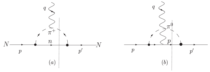
Figure 4: Absorptive part of the $\gamma NN$ vertex with final nucleon off the mass shell, used in the sideways dispersion relation for the nucleon a.m.m.. Diagram (a) : $\pi^{+}n$ loop where the photon couples to the $\pi^{+}$; diagram (b) : $\pi^{0}p$ loop where the photon couples to the charge of the proton. The vertical dotted lines indicate that the $\pi N$ intermediate state is taken on shell.

where $G_{N}^{(+)}$ is now the appropriate half-off-shell form factor for the nucleon, cf. Eq. (29). The absorptive part of this form factor to one loop is obtained by computing the indicated cuts of the graphs in Fig. 4. For instance, the result for the proton can be written as:

$$\mathrm{Im}\,G_{p}^{(+)}=-\frac{M^{2}}{e^{2}}\left[\Delta\sigma_{s1p}^{(\pi^{+}n)}+\Delta\sigma_{s1p}^{(\pi^{0}p)}\right],$$ (45)

where the first term is equivalent to the contribution of Fig. 4 (a), whereas the second term represents Fig. 4 (b). Explicit forms of these functions $\Delta\sigma_{s}$ are listed in the Appendix B. Making the connection with the linearized GDH sum rule, we find that these $\Delta\sigma_{s}$ can equivalently be determined by computing the interference of the Born pion-photoproduction graphs (Fig. 3) and the $s$-channel graph with a Pauli-coupling insertion [first graph in Fig. 3(b)].

Note that $\Delta\sigma_{s1p}^{(\pi^{+}n)}$ entering the above sideways dispersion relation is exactly the same as the corresponding integrand $\Delta\sigma_{1p}^{(\pi^{+}n)}$ entering the linearized GDH sum rule of Eq. (41b). The term $\Delta\sigma_{s1p}^{(\pi^{0}p)}$ in the integrand of Eq. (44) on the other hand is different from the corresponding term $\Delta\sigma_{1p}^{(\pi^{0}p)}$ in Eq. (41b). However, one can easily check that upon integration both integrands give the same contribution to the magnetic moments. We have verified this result for both pseudo-scalar and pseudo-vector $\pi NN$ couplings.

In Appendix C, we, for completeness, list all the expressions for the second derivatives of the GDH cross-sections for different single-pion production channels in Born approximation.

VI Chiral corrections to nucleon polarizabilities

It is well-known that the Heavy-Baryon ChPT (HBChPT) at order ${\cal O}(p^{3})$ yields the prediction for the electric and magnetic polarizabilities of the nucleon:

$$\alpha_{E}^{(HBLO)}=\frac{5\pi\alpha_{em}}{6\,m_{\pi}}\left(\frac{g_{A}}{4\pi f_{\pi}}\right)^{2}=12.2\times 10^{-4}~{}\mbox{fm}^{3},$$ (46a)

$$\beta_{M}^{(HBLO)}=\frac{\pi\alpha_{em}}{12\,m_{\pi}}\left(\frac{g_{A}}{4\pi f_{\pi}}\right)^{2}=1.2\times 10^{-4}~{}\mbox{fm}^{3}\,,$$ (46b)

where $g_{A}\simeq 1.26$, $f_{\pi}\simeq 92.4$ MeV. Here the couplings are related to the $\pi NN$ coupling constant used in the previous section via the Goldberger-Treiman relation: $g_{A}/f_{\pi}=g/M$.

Eqs. 46 are a true prediction of ${\cal O}(p^{3})$ HBChPT (there are no counter-terms at this order) and turn out to be in remarkable agreement with experiment, e.g., for the proton polz :

$$\alpha_{E}^{(exp)} = 12.1\pm 0.3\,\mbox{(stat)}\mp 0.4\,\mbox{(syst)}\pm 0.3\,\mbox{(mod)}\,\,[\times 10^{-4}\,\,{\rm fm}^{3}]\,,$$ (47a)

$$\beta_{M}^{(exp)} = 1.6\pm 0.4\,\mbox{(stat)}\pm 0.4\,\mbox{(syst)}\pm 0.4\,\mbox{(mod)}\,\,[\times 10^{-4}\,\,{\rm fm}^{3}]\,.$$ (47b)

By using forward sum rules, we can discuss here only the sum of the electric and magnetic polarizabilities. On the experimental side, a recent determination from the Baldin’s sum gives Bab98 :

$$(\alpha_{E}+\beta_{M})_{p}^{exp} = (13.69\pm 0.14)\times 10^{-4}~{}{\rm{fm}}^{3}\ ,$$

$$(\alpha_{E}+\beta_{M})_{n}^{exp} = (14.40\pm 0.66)\times 10^{-4}~{}{\rm{fm}}^{3}\ ,$$ (48)

for proton and neutron, respectively.

In order to find the leading order relativistic prediction of chiral loops we have computed the unpolarized total cross-sections, corresponding to the Born graphs of single-pion photoproduction :

$$\sigma^{(\pi^{0}p)} = \frac{\pi C}{M\omega^{3}}\,\left\{[\omega^{2}-\mu^{2}\alpha\,s]\,\ln\frac{\alpha+\lambda}{\alpha-\lambda}+2\lambda\left[\omega^{2}(\alpha-2)1+s\mu^{2}\right]\right\},$$

$$\sigma^{(\pi^{+}n)} = \frac{2\pi C}{M\omega^{3}}\,\left\{-\beta\,s\,\mu^{2}\ln\frac{\beta+\lambda}{\beta-\lambda}+2\lambda\,(\alpha\,\omega^{2}+s\,\mu^{2})\right\},$$ (49a)

$$\sigma^{(\pi^{0}n)} = 0,$$

$$\sigma^{(\pi^{-}p)} = \frac{2\pi C}{M\omega^{3}}\,\left\{\omega^{2}\ln\frac{\alpha+\lambda}{\alpha-\lambda}-\mu^{2}(s\beta-\mu^{2}M^{2})\,\ln\frac{\beta+\lambda}{\beta-\lambda}\,\frac{\alpha+\lambda}{\alpha-\lambda}+2s\mu^{2}\lambda\right\}.$$ (49b)

Substituting these expressions into the Baldin SR, Eq. (6), we obtain:

$$(\alpha_{E}+\beta_{M})_{p}^{(RLO)} = \frac{e^{2}g^{2}}{16\pi^{3}M^{3}}\left\{[3(1-4\mu^{2}+2\mu^{4})+\mbox{$\frac{1}{3}$}\mu^{2}]\ln\mu+\frac{406-737\mu^{2}+304\mu^{4}-36\mu^{6}}{6(4-\mu^{2})^{2}}\right.$$ (50a)

$$+ \left.\frac{44-788\mu^{2}+1500\mu^{4}-899\mu^{6}+215\mu^{8}-18\mu^{10}}{3\mu(4-\mu^{2})^{5/2}}\,{\rm arctg}{\sqrt{\frac{4}{\mu^{2}}-1}}\,\right\}\,,$$

$$(\alpha_{E}+\beta_{M})_{n}^{(RLO)} = \!\frac{e^{2}g^{2}}{16\pi^{3}M^{3}}\left\{\ln\mu\right.$$

$$+ \left.\frac{1}{(4-\mu^{2})^{2}}\left[\frac{2(2-3\mu^{2})(11-5\mu^{2})-3\mu^{6}}{3\mu\sqrt{4-\mu^{2}}}\,{\rm arctg}{\sqrt{\frac{4}{\mu^{2}}-1}}+5-\mu^{2}\right]\right\}.$$

Note that an identical result is obtained in the conventional one-loop Feynman diagram calculation BKMalbeloop ; Metz96 . The corresponding (chiral) $\mu$-expansion reads:

$$(\alpha_{E}+\beta_{M})_{p}^{(RLO)} = \frac{e^{2}g^{2}}{(4\pi)^{2}M^{3}}\frac{11}{48\mu}\left\{1+\frac{48(4+3\ln\mu)}{11\pi}\mu-\frac{1521}{88}\mu^{2}+\ldots\right\},$$ (51a)

$$(\alpha_{E}+\beta_{M})_{n}^{(RLO)} = \frac{e^{2}g^{2}}{(4\pi)^{2}M^{3}}\frac{11}{48\mu}\left\{1+\frac{4(1+12\ln\mu)}{11\pi}\mu-\frac{117}{88}\mu^{2}+\ldots\right\},$$ (51b)

or, numerically (using $$g^{2}/4\pi=13.8 M=0.9383 \mu=0.148$$, GeV, ),

$$(\alpha_{E}+\beta_{M})_{p}^{(RLO)} = 14.5-5.2-5.5+\ldots=3.8,$$ (51c)

$$(\alpha_{E}+\beta_{M})_{n}^{(RLO)} = 14.5-5.4-0.4+\ldots=8.7,$$ (51d)

in units of $10^{-4}\,\,{\rm fm}^{3}$. As one can clearly see, the fully relativistic leading order result is substantially different from the non-relativistic (heavy-baryon) limit. The higher order corrections, which are suppressed by $m_{\pi}/M\simeq 1/7$, and hence are expected to be small, appear with large coefficients and generate a substantial modification of the leading order result. This (relativistic) effect is likely to allow one to accommodate the relatively large $\Delta$-resonance contribution to the magnetic polarizability Pas05 .

For the forward spin polarizability, Bernard, Hemmert and Meißner obtainbhm  :

$$\gamma_{0}^{(p)}=\frac{e^{2}g^{2}}{16\pi^{3}\mu^{2}}\left[1-\frac{21\,\pi\,\mu}{8}-\left(20+26\,\ln\mu\right){\mu}^{2}+\frac{1875\,\pi\,{\mu}^{3}}{64}+\ldots\right],$$ (52)

while, using the sum rule of Eq. 8, we obtain :

$$\gamma_{0}^{(p)}=\frac{e^{2}g^{2}}{16\pi^{3}\mu^{2}}\left[1-\frac{21\,\pi\,\mu}{8}-\left(\frac{59}{2}+26\,\ln\mu\right){\mu}^{2}+\frac{1875\,\pi\,{\mu}^{3}}{64}+\ldots\right].$$ (53)

The difference between both expressions is confined to the analytic terms. The sum rule calculation has analyticity built in explicitly.

VII Chiral extrapolations

It is instructive to examine the chiral behavior of the one-loop result for the nucleon magnetic moment. Expanding Eq. (43) around the chiral limit ($m_{\pi}=0$) we have

$$\kappa_{p}^{\rm(loop)} = \frac{g^{2}}{(4\pi)^{2}}\left\{1-2\pi\mu-2\,(2+5\ln\mu)\,\mu^{2}+\frac{21\pi}{4}\,\mu^{3}+O(\mu^{4})\right\},$$ (54a)

$$\kappa_{n}^{\rm(loop)} = \frac{g^{2}}{(4\pi)^{2}}\left\{-4+2\pi\mu-2\,(1-2\ln\mu)\,\mu^{2}-\frac{3\pi}{4}\,\mu^{3}+O(\mu^{4})\right\}.$$ (54b)

Apart from the first term, the constant, which renormalizes the counter term as described above, this expansion corresponds with the heavy-baryon expansion. The term linear in pion mass (recall that $\mu=m_{\pi}/M$) is the well-known leading nonanalytic (LNA) correction.

On the other hand, expanding the same expressions around the large $m_{\pi}$ limit we find

$$\kappa_{p}^{\rm(loop)} = \frac{g^{2}}{(4\pi)^{2}}\,(5-4\ln\mu)\frac{1}{\mu^{2}}+O(\mu^{-4}),$$ (55a)

$$\kappa_{n}^{\rm(loop)} = \frac{g^{2}}{(4\pi)^{2}}\,2(3-4\ln\mu)\frac{1}{\mu^{2}}+O(\mu^{-4}).$$ (55b)

What is intriguing here is that the one-loop correction to the nucleon a.m.m. for heavy quarks behaves as $1/m_{quark}$ (where $m_{quark}\sim m_{\pi}^{2})$, precisely as expected from a constituent quark-model picture Leinweber:1998ej . Here this is a result of subtle cancellations in Eq. (43) taking place for large values of $m_{\pi}$. In contrast, the infrared regularization procedure Kubis:2000zd gives the result which exhibits pathological behavior with increasing pion mass and diverges for $m_{\pi}=2M$.

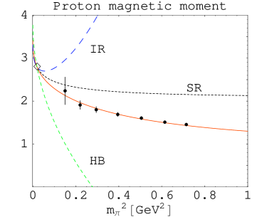
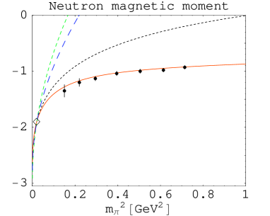
Figure 5: Chiral behavior of proton and neutron magnetic moments (in nucleon magnetons) to one loop compared with lattice data. “SR” (dotted lines): our one-loop relativistic result, “IR” (blue long-dashed lines): infrared-regularized relativistic result, “HB” (green dashed lines): LNA term in the heavy-baryon expansion. Red solid lines: single-parameter fit based on our SR result. Data points are results of lattice simulations. The open diamonds represent the experimental values at the physical pion mass.

Since the expressions in Eq. (43) both have the correct large and small $m_{\pi}$ behavior they should be better suited for the chiral extrapolations of lattice results than the usual heavy-baryon expansions or the “infrared-regularized” relativistic theory. This point is clearly demonstrated by Fig. 5, where we plot the $m_{\pi}$-dependence of the full [Eq. (43)], heavy-baryon, and infrared-regularizationKubis:2000zd leading order result for the magnetic moment of the proton and the neutron, in comparison to recent lattice dataZan04 . In presenting these results we have added a constant shift (counter-terms $\kappa_{0}$) to the magnetic moments, i.e.,

$$\mu_{p} = (1+\kappa_{0p}+\kappa_{p}^{\rm(loop)})(e/2M),$$ (56)

$$\mu_{n} = (\kappa_{0n}+\kappa_{n}^{\rm(loop)})(e/2M)$$ (57)

and fitted them to the known experimental value of the magnetic moments at the physical pion mass, $\mu_{p}\simeq 2.793$ and $\mu_{n}\simeq-1.913$, shown by the open diamonds in the figure. For the value of the $\pi NN$ coupling constant we have used $g^{2}/4\pi=13.5$. The $m_{\pi}$-dependence away from the physical point is then a prediction of the theory. The figure clearly shows that the SR-motivated extrapolation, shown by the dotted lines, is in a good agreement with the $m_{\pi}$-dependence obtained in lattice gauge simulations.

It is therefore tempting to use the SR results for the parametrization of lattice data. For example, we consider the following elementary two-parameter form:

$$\mu_{p} = \left(1+\frac{\tilde{\kappa}_{0p}}{1+a_{p}m_{\pi}^{2}}+\kappa_{p}^{\rm(loop)}\right)\frac{e}{2M},$$ (58a)

$$\mu_{n} = \left(\frac{\tilde{\kappa}_{0n}}{1+a_{n}m_{\pi}^{2}}+\kappa_{n}^{\rm(loop)}\right)\frac{e}{2M}\,,$$ (58b)

where $\tilde{\kappa}_{0p}$ and $\tilde{\kappa}_{0n}$ are fixed to reproduce the experimental magnetic moments at the physical $m_{\pi}$. The parameter $a$ can be fitted to lattice data. The solid curves in Fig. 5 represent the result of such a single parameter fit to the lattice data of Ref. Zan04 for the proton and neutron respectively, where $a_{p}=1.6/M^{2}$ and $a_{n}=1.05/M^{2}$, and $M$ is the physical nucleon mass. This parametrization incorporates the experimental value at the physical pion mass and reproduces very well the trend of the lattice data.

We would like to stress here that at larger pion masses the ChPT result should be interpreted as merely a convenient parametrization of lattice data, not as a prediction of the theory. In this way one obtains a parametrization which fits the lattice data at larger values of $m_{\pi}$ and has the correct dependence at lower values of $m_{\pi}$. Apparently, the relativistic ChPT result which is consistent with analyticity provides the most convenient ground for the fit to lattice data, because it has an $1/m_{q}$ behavior at larger values of $m_{\pi}$. It is useful to test the consistency of lattice simulations at larger $m_{\pi}$ and the experimental values based on such a single-free-parameter form which encodes the correct chiral behavior at low pion masses.

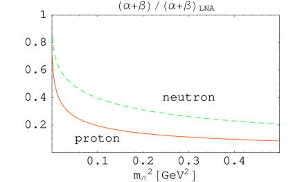
Figure 6: The ratio of the one-loop proton (solid curves) and neutron (dashed curves) forward polarizabilities to their LNA terms in the heavy-baryon expansion.

The importance of the relativistic effects is even more emphasized in the polarizabilities. In Fig. 6 we have plotted the ratio of one-loop $\alpha_{E}+\beta_{M}$, Eq. (50), to its leading non-analytic term [first term in the expansion Eq. (51)]. Recently, the electric and magnetic polarizabilities of hadrons have been calculated in lattice QCD using the external field method Christensen:2004ca ; Zhou:2002km . This method amounts to extract the electric and magnetic polarizabilities of hadrons from the quadratic term in the mass shift in an external electromagnetic field. The low statistics, pioneering results have so far been obtained for pion masses above 450 MeV. As higher statistics calculations will become available in the near future Lee05 ; Zanotti05 , our sum rule calculation of the pion mass dependence of the forward polarizabilities provides a way to connect these next generation lattice results to experiment.

VIII Prospects for the future

In this section we outline a procedure for two-loop calculations of the a.m.m. by using derivative forms of the GDH SR. Again, the GDH SR in its original form is practically unsuitable for such calculations, because in order to compute $\kappa$ in, e.g., QED to order $\alpha_{em}^{2}$ one needs to compute the photoabsorption cross-sections to order $\alpha_{em}^{5}$—also to two loops! By contrast, using the derivative trick of Sect. III, we will need the (derivatives of) cross-sections up to order $\alpha_{em}^{3}$ only—one loop forms.

Introducing the ‘trial’ value of $\kappa_{0}$, such that the full a.m.m. is defined as $\kappa=\kappa_{0}+\delta\kappa$, and the GDH cross-section can be written as

$$\Delta\sigma(\kappa_{0})=\Delta\sigma+\kappa_{0}\,\Delta\sigma^{\prime}+\mbox{\small{$\frac{1}{2}$}}\kappa_{0}^{2}\,\Delta\sigma^{\prime\prime}+\ldots\,,$$ (59)

the first and second derivatives of the GDH SR at $\kappa_{0}=0$ read, respectively:

$$\delta\kappa+\delta\kappa\,\delta\kappa^{\prime}=\frac{M^{2}}{4\pi^{2}\alpha_{em}}\int\limits_{0}^{\infty}\!\frac{d\omega}{\omega}\,\Delta\sigma^{\prime}$$ (60a)

$$2\delta\kappa^{\prime}+(\delta\kappa^{\prime})^{2}+\delta\kappa\,\delta\kappa^{\prime\prime}=\frac{M^{2}}{4\pi^{2}\alpha_{em}}\int\limits_{0}^{\infty}\!\frac{d\omega}{\omega}\,\Delta\sigma^{\prime\prime}$$ (60b)

Now, consider Eq. (60a) at order $\alpha_{em}^{2}$:

$$\delta\kappa^{(2)}+\delta\kappa^{(1)}\,\delta\kappa^{\prime(1)}=\frac{M^{2}}{4\pi^{2}\alpha_{em}}\int\limits_{0}^{\infty}\!\frac{d\omega}{\omega}\,\Delta\sigma^{\prime(3)}\,,$$ (61)

where the superscript indicates the order of $\alpha_{em}$ to which the quantity is considered. We can use Eq. (60a) and Eq. (60b) at order $\alpha_{em}$ to obtain, respectively:

$$\delta\kappa^{(1)} = \frac{M^{2}}{4\pi^{2}\alpha_{em}}\int\limits_{0}^{\infty}\!\frac{d\omega}{\omega}\,\Delta\sigma^{\prime(2)}\,,$$ (62a)

$$\delta\kappa^{\prime(1)} = \frac{M^{2}}{8\pi^{2}\alpha_{em}}\int\limits_{0}^{\infty}\!\frac{d\omega}{\omega}\,\Delta\sigma^{\prime\prime(2)}\,.$$ (62b)

Substituting these in Eq. (61) we find the linearized GDH sum rule at order $\alpha_{em}^{2}$:

$$\delta\kappa^{(2)}=\frac{M^{2}}{4\pi^{2}\alpha_{em}}\left[\int\limits_{0}^{\infty}\!\frac{d\omega}{\omega}\,\Delta\sigma^{\prime\,(3)}-\frac{M^{2}}{8\pi^{2}\alpha_{em}}\left(\int\limits_{0}^{\infty}\!\frac{d\omega}{\omega}\,\Delta\sigma^{\prime\,(2)}\right)\,\left(\int\limits_{0}^{\infty}\!\frac{d\omega}{\omega}\,\Delta\sigma^{\prime\prime\,(2)}\right)\right]\,,$$ (63)

and, using this sum rule one can obtain all two-loop corrections to the a.m.m. by computing the first derivative of the GDH cross-section $\Delta\sigma^{\prime}$ at one-loop and tree level, and a second derivative of the GDH cross-section $\Delta\sigma^{\prime\prime}$ at tree level.

For the QED case we have thus far worked out the required derivatives at tree level only. The first derivative is given in Eq. (26), while the second derivative is given by:

$$\Delta\sigma^{{}^{\prime\prime}(2)}=\frac{2\pi{\alpha_{em}^{2}}}{M^{2}x}\,\left[-\frac{9+29\,x+18\,x^{2}-10\,x^{3}}{{\left(1+2\,x\right)}^{2}}+\left(1+\frac{9}{2\,x}\right)\,\log(1+2\,x)\right]\,,$$ (64)

with $x=\omega/M$. As already shown, the dispersion integral over the first derivative yields the Schwinger correction, cf. Eq. (27). The integral over the second derivative is divergent and to evaluate it we introduce an ultraviolet cutoff ${\Lambda}\gg M$:

$$\frac{1}{\pi}\int\limits_{0}^{\Lambda}\!\frac{d\omega}{\omega}\,\Delta\sigma^{\prime\prime\,(2)}=\frac{\alpha_{em}^{2}}{M^{2}}\left(5\log\frac{2{\Lambda}}{M}-6\right)\,.$$ (65)

The same cutoff needs to be introduced in the first integral of the sum rule Eq. (63), such that the total result is independent of the cutoff. Thus, in QED we obtain

$$\delta\kappa^{(2)}=\frac{M^{2}}{4\pi^{2}\alpha_{em}}\int\limits_{0}^{\Lambda}\!\frac{d\omega}{\omega}\,\Delta\sigma^{\prime\,(3)}-\frac{\alpha_{em}^{2}}{16\pi^{2}}\left(5\log\frac{2{\Lambda}}{M}-6\right)\,.$$ (66)

In order to complete this two-loop calculation of the electron a.m.m. in QED one would need to evaluate the first derivative $\Delta\sigma^{\prime}$ at order $\alpha_{em}^{3}$ which is given by the interference of the tree-level and one-loop Compton scattering amplitudes, as well as by the tree-level bremsstrahlung and pair production mechanisms, all with one insertion of the Pauli vertex. Diagrammatically this calculation is depicted in Fig. 7. It is a future challenge to perform such calculation and to verify whether the linearized GDH SR reproduces the two-loop result obtained by usual techniques twoloopQED :

$$\delta\kappa^{(2)}=\frac{\alpha_{em}^{2}}{\pi^{2}}\left[\frac{197}{144}+\frac{\pi^{2}}{2}(\mbox{\small{$\frac{1}{6}$}}-\log 2)+\frac{3}{4}\,\zeta(3)\right]\simeq-0.328479\,(\alpha_{em}^{2}/\pi^{2})\,.$$ (67)

This would be an exact test of the GDH SR at the two-loop level.

In the case of the nucleon, sum rules analogous to Eq. (61) may provide a more efficient method to do a two-loop calculation for the nucleon a.m.m.or for the forward spin polarizability, since much is already known about the one-loop ChPT amplitudes of pion-photoproduction BKMLee , which are required in such a calculation.

IX Conclusion

Direct application of QCD to low energy hadronic physics is made challenging by the feature that the quark/gluon degrees of freedom in terms of which QCD is couched are confined within hadronic systems. Nevertheless, the chiral EFT of QCD—chiral perturbation theory—allows a predictive description of the low-energy hadronic reactions. Also, by focusing on the chiral structure of the underlying Lagrangian such EFT methods permit one to make a link to lattice QCD calculations, even in the case where the mass of the underlying Goldstone bosons is considerably heavier than found experimentally. These are the two fronts which at present make the chiral EFT indispensable in relating QCD to low-energy observables. On the other hand there remain significant problems. Indeed, most such calculations involving nucleons are carried out at low orders in so-called heavy baryon chiral perturbation theory, which involves an expansion in powers of the inverse nucleon mass. On the other hand, we have demonstrated above by simple examples involving the nucleon magnetic moment and polarizabilities, that manifestly relativistic calculations, which include chiral corrections to all orders in $\mu=m_{\pi}/M_{N}$, do a better job than the “heavy-baryon” ones on both fronts in capturing the full implications of the theory.

For this reason it is important to have at one’s disposal methods which allow such all orders evaluation of experimental quantities. This can in principle be achieved using conventional relativistic chiral loop calculations, but the price in terms of the number of diagrams which must be evaluated is high. For example, a one-loop evaluation of the nucleon polarizability involves fifty-two such diagrams for the proton and twenty-two for the neutronKMB ! Above we have presented an alternative approach, involving the use of dispersion relations and their related sum rules. The calculations done in this work were based on real-Compton-scattering sum rules, such as GDH and Baldin sum rules. However, the results are identical to what one would obtain in the usual loop calculations, provided no manipulations, such as infrared regularization which change the analytic structure are made. As is shown in the works of Gegelia et al. Geg99 , there is no problem with power counting in this straightforward formulation of covariant ChPT, if the renormalization is performed in a suitable way. Both the infrared-regularized and the straightforward formulation of relativistic baryon ChPT resum the nominally higher-order relativistic effects, albeit differently. We stress that the resummation in the straightforward version is done in accordance with the principle of analyticity.

We demonstrated above the utility of taking derivatives of the GDH sum rule, in order to convert it to forms which are sometimes more calculationally robust. We showed that in some cases these modified versions of the sum rules are equivalent to sideways dispersion relations, which involve taking the final (or initial) nucleon four–momentum off-shell. Using such relations, we straightforwardly evaluated fully relativistic nucleon magnetic moments and polarizabilities, using only tree level inputs and showed that they were fully equivalent to values obtained via much more labor-intensive loop techniques. We showed that such methods should also permit a future evaluation of the two loop electron anomalous magnetic moment.

The successes demonstrated above suggest an obvious direction for future work. In particular, the use of dispersive methods would seem to be ideal for a simplified way to perform two-loop evaluations. An obvious first test would be to use one-loop corrected photoproduction amplitudes in order to produce corresponding one-loop photoabsorption cross sections, which can in turn be used to generate two-loop values of polarizabilities and of magnetic moments which are relativistically correct. These can then be compared to ongoing calculations at two loop in the heavy baryon expansion for the forward spin polarizability and with the “experimental” value obtained from the sum rule. In conclusion there is much which can be done with such methods, and many future applications can be envisioned.

Appendix A Calculation of photoproduction cross-sections

We write the pion photoproduction amplitude in the following general form:

$$T_{\pi\gamma}=\bar{u}(p^{\prime})\,\sum_{i=1}^{4}A_{i}(s,t)\,O_{i}(\varepsilon)\,u(p)\,,$$ (68)

where $A$’s are the invariant amplitudes and $O$’s are given by

$$O_{1} = \gamma_{5}\,,$$

$$O_{2} = \varepsilon\cdot\gamma\cdot q\,\gamma_{5}\,,$$

$$O_{3} = \gamma\cdot\varepsilon\,\gamma_{5}\,,$$ (69)

$$O_{4} = \gamma\cdot q\,\gamma_{5}\,,$$

with $\varepsilon\cdot\gamma\cdot q\equiv\mbox{\small{$\frac{1}{2}$}}[\gamma_{\mu},\gamma_{\nu}]\,\varepsilon^{\mu}q^{\nu}$.

The total and double-polarized cross-sections are given respectively by

$$\sigma = \frac{2\pi\lambda}{x}\sum_{i,j=1}^{4}\int^{1}_{-1}d(\cos\theta)\,Y_{ij}\,A_{i}\,A_{j},$$ (70)

$$\Delta\sigma = \frac{2\pi\lambda}{x}\sum_{i,j=1}^{4}\int^{1}_{-1}d(\cos\theta)\,Z_{ij}\,A_{i}\,A_{j},$$ (71)

with $\theta$ the scattering angle and

$$Y_{ij} = {\rm Tr}\left[{\Lambda}^{(+)}(p/^{\prime})\,O_{i}\,{\Lambda}^{(+)}(p/)\,O_{j}\right]\,,$$ (72)

$$Z_{ij} = {\rm Tr}\left[{\Lambda}^{(+)}(p/^{\prime})\,O_{i}\,{\Lambda}^{(+)}(p/)\,{\vec{\Sigma}}\cdot{\vec{p}}\,O_{j}\right]\,,$$ (73)

where $\vec{\Sigma}=\gamma_{0}\gamma_{5}\vec{\gamma}$, $\vec{p}$ is the 3-momentum of the incoming nucleon, and the projection operator ${\Lambda}^{(+)}$ is defined in Eq. (30). More explicitly, the traces are given by

$$Y = \left(\begin{array}[]{cccc}\mbox{\small{$\frac{1}{2}$}}\bar{t}&-x\xi&\xi&y-x\\ -x\xi&-2xy&x+y&0\\ \xi&x+y&-2+\mbox{\small{$\frac{1}{2}$}}\bar{t}&-x\xi\\ y-x&0&-x\xi&-2xy\end{array}\right),$$ (78)

$$Z = \left(\begin{array}[]{cccc}0&x\xi&-\xi&0\\ x\xi&2xy&-x-y&0\\ -\xi&-x-y&2-\mbox{\small{$\frac{1}{2}$}}\bar{t}&x\xi\\ 0&0&x\xi&0\end{array}\right),$$ (83)

where $x=(s-M^{2})/2M^{2}=\omega/M$, $y=(M^{2}-u)/2M^{2}$, $\xi=p^{\prime}\cdot\varepsilon=\lambda\sqrt{\bar{s}}\,\sin\theta$, $\bar{s}=s/M^{2}$, $\bar{t}=t/M^{2}$ ($s$, $t$ and $u$ are the Mandelstam variables).

In the notations of Eq. (37) the expression for the total cross-section of pion photoproduction in Born approximation, including the nucleon a.m.m. terms, takes the following form:

$$\sigma^{(\pi^{0}p)} = \frac{\pi C}{M^{2}x^{3}}\,\left\{[x^{2}(1+2\kappa_{p}+\mbox{\small{$\frac{1}{2}$}}\kappa_{p}^{2})-\mu^{2}\alpha\,\bar{s}]\,\ln\frac{\alpha+\lambda}{\alpha-\lambda}\right.$$

$$+ \left.2\lambda\left[x^{2}(\alpha-2)(1+\kappa_{p})^{2}+\bar{s}\mu^{2}+\mbox{\small{$\frac{1}{2}$}}\kappa_{p}^{2}\alpha\,\bar{s}\right]\right\},$$

$$\sigma^{(\pi^{+}n)} = \frac{2\pi C}{M^{2}x^{3}}\,\left\{-\beta\,\bar{s}\,\mu^{2}\,\ln\frac{\ \beta+\lambda}{\beta-\lambda}+2\lambda\,(\alpha\,x^{2}+\bar{s}\,\mu^{2})\right.$$ (84)

$$+ x^{2}\,\lambda\,\left[-2(\kappa_{p}+\kappa_{n})\,\beta+(\kappa_{p}^{2}+\kappa_{n}^{2})(x\beta-\mbox{\small{$\frac{1}{2}$}}\mu^{2})\right]$$

$$+ \left.x^{2}\,\kappa_{p}\,\kappa_{n}\left[\mbox{\small{$\frac{1}{2}$}}\ln\frac{\alpha+\lambda}{\alpha-\lambda}-\lambda(2-\alpha\,\bar{s}+2(1+x)\beta-\mu^{2})\right]\right\},$$

$$\sigma^{(\pi^{0}n)} = \frac{\pi C}{M^{2}x}\kappa_{n}^{2}\left\{\mbox{\small{$\frac{1}{2}$}}\ln\frac{\alpha+\lambda}{\alpha-\lambda}+[-4+(2+\bar{s})\,\alpha\,]\,\lambda\right\},$$

$$\sigma^{(\pi^{-}p)} = \frac{2\pi C}{M^{2}x^{3}}\,\left\{x^{2}\ln\frac{\alpha+\lambda}{\alpha-\lambda}-\mu^{2}(\bar{s}\,\beta-\mu^{2})\,\ln\frac{\beta+\lambda}{\beta-\lambda}\,\frac{\alpha+\lambda}{\alpha-\lambda}+2\bar{s}\mu^{2}\lambda\right.$$

$$+ x^{2}(\kappa_{p}+\kappa_{n})\left(2\lambda-\ln\frac{\alpha+\lambda}{\alpha-\lambda}\right)+x^{2}(\kappa_{p}^{2}+\kappa_{n}^{2})(x\beta-\mbox{\small{$\frac{1}{2}$}}\mu^{2})$$

$$+ \left.x^{2}\kappa_{p}\kappa_{n}\left[(1+\beta)\lambda+\frac{1}{2}\ln\frac{\alpha+\lambda}{\alpha-\lambda}\right]\right\}.$$

Appendix B First derivatives of GDH Born cross-sections of pion photoproduction

In this appendix we present explicit expressions for the $\Delta\sigma_{1}$ cross-sections for the pion photoproduction on the proton.

B.1 Pseudo-vector coupling

Computing the Born graph contribution with the pseudo-vector $\pi NN$ coupling we obtain:

$$\Delta\sigma_{1p}^{(\pi^{0}p)} = \frac{\pi C}{M^{2}x^{2}}\left\{(2\alpha\bar{s}+1-x)\ln\frac{\alpha+\lambda}{\alpha-\lambda}-2\lambda\,[x(\alpha-2-\mu^{2})+\bar{s}(2+\alpha)]\right\}$$ (85)

$$= \Delta\sigma^{(\pi^{0}p)}+\frac{2\pi C}{M^{2}x}\,\lambda\,\mu^{2}$$

$$\Delta\sigma_{1n}^{(\pi^{0}p)} = \Delta\sigma_{2nn}^{(\pi^{0}p)}=\Delta\sigma_{2pn}^{(\pi^{0}p)}=0$$ (86)

$$\Delta\sigma_{1p}^{(\pi^{+}n)} = \frac{\pi C}{M^{2}x}\,\left\{-\mu^{2}\ln\frac{\beta+\lambda}{\beta-\lambda}+2\lambda(\bar{s}\,\beta-x\alpha)\right\},$$ (87)

$$\Delta\sigma_{1n}^{(\pi^{+}n)} = \Delta\sigma_{1p}^{(\pi^{+}n)}-\frac{4\pi C}{M^{2}x^{2}}\,\alpha\,\bar{s}\,\lambda\,.$$ (88)

where the notations are detailed in Eq. (37), and $\Delta\sigma^{(\pi^{0}p)}$ is given in Eq. (36).

B.2 Pseudo-scalar coupling

In the case of pseudo-scalar $\pi NN$ coupling the expressions are different.

$$\Delta\sigma_{1p}^{(\pi^{0}p)} = \frac{\pi C}{M^{2}x^{2}}\left\{2\lambda\,(\alpha-\bar{s}-3+\mu^{2})+(3-\mu^{2})\ln\frac{\alpha+\lambda}{\alpha-\lambda}\right\},$$ (89)

$$\Delta\sigma_{1n}^{(\pi^{0}p)} = \Delta\sigma_{2nn}^{(\pi^{0}p)}=\Delta\sigma_{2pn}^{(\pi^{0}p)}=0$$ (90)

$$\Delta\sigma_{1p}^{(\pi^{+}n)} = \Delta\sigma_{1n}^{(\pi^{+}n)}=\frac{4\pi C}{M^{2}x}\lambda\,\beta.$$ (91)

Note, however, the contribution of these cross-sections to the linearized GDH sum rule Eq. (41) is exactly the same in both the pseudo-vector and pseudo-scalar cases.

B.3 Integrands of the sideways dispersion relation

The integrands entering the sideways dispersion relations of Eq. (44) for the proton a.m.m. are given by :

$$\Delta\sigma_{s1p}^{(\pi^{+}n)} = \Delta\sigma_{1p}^{(\pi^{+}n)},$$ (92)

$$\Delta\sigma_{s1p}^{(\pi^{0}p)} = \frac{\pi C}{M^{2}x}\left\{2\lambda\,(1+\beta)-\ln\frac{\alpha+\lambda}{\alpha-\lambda}\right\}.$$ (93)

Appendix C Second derivatives of GDH Born cross-sections of pion photoproduction

In this appendix we list the expressions for the second derivatives of the GDH cross section, defined as:

$$\Delta\sigma_{2ij}=\left.\frac{\partial}{\partial\kappa_{0i}}\frac{\partial}{\partial\kappa_{0j}}\Delta\sigma(\omega;\,\kappa_{0p},\,\kappa_{0n})\right|_{\kappa_{0p}=\kappa_{0n}=0}\,.$$ (94)

Using the pseudo-vector coupling, we obtain:

$$\Delta\sigma_{2pp}^{(p)} = \Delta\sigma_{2nn}^{(n)}=\frac{2\pi C}{M^{2}x}\left\{\lambda(4-2x\beta-2\alpha+\mu^{2})-\ln\frac{\alpha+\lambda}{\alpha-\lambda}\right\},$$ (95)

$$\Delta\sigma_{2nn}^{(p)} = \Delta\sigma_{2pp}^{(n)}=\frac{2\pi C}{M^{2}x}\left\{\lambda[2(\bar{s}+x)\alpha-2x+\mu^{2}]-\ln\frac{\alpha+\lambda}{\alpha-\lambda}\right\},\qquad$$ (96)

$$\Delta\sigma_{2pn}^{(p)} = \Delta\sigma_{2pn}^{(n)}=\frac{\pi C}{M^{2}x}\left\{2\lambda[-2\beta(1+x)+\bar{s}\alpha-2+\mu^{2}]+\ln\frac{\alpha+\lambda}{\alpha-\lambda}\right\}.\qquad$$ (97)

Using the pseudo-scalar coupling, we obtain:

$$\mbox{\small{$\frac{1}{2}$}}\Delta\sigma_{2pp}^{(\pi^{0}p)} = \Delta\sigma_{2pn}^{(\pi^{+}n)}=\frac{\pi C}{M^{2}x}\left\{2\lambda\,(1+\beta)-\ln\frac{\alpha+\lambda}{\alpha-\lambda}\right\},$$ (98)

$$\Delta\sigma_{2pp}^{(\pi^{+}n)} = \frac{2\pi C}{M^{2}x}\lambda\,(\mu^{2}-2x\beta)=\frac{4\pi C}{M^{2}x}\lambda\,(\beta-\alpha x)\,,$$ (99)

$$\Delta\sigma_{2nn}^{(\pi^{+}n)} = \frac{2\pi C}{M^{2}x}\left\{\lambda\,(1+\beta+\alpha\,\bar{s})-\ln\frac{\alpha+\lambda}{\alpha-\lambda}\right\}.$$ (100)

Figure 1: Tree-level Compton scattering amplitude in QED.

Figure 2: Tree-level Compton scattering graphs with one Pauli-coupling insertion. The circled vertex corresponds to the Pauli coupling.

Figure 3: Tree-level pion photoproduction graphs. The circled vertex corresponds to the Pauli coupling.

Figure 7: Interference contributions which give rise to the $\Delta\sigma^{\prime(3)}$ in QED. The circled vertex corresponds to the Pauli coupling.

References

• (1) S. B. Gerasimov, Sov. J. Nucl. Phys.  2, 430 (1966) [Yad. Fiz.  2, 598 (1966)]; S. D. Drell and A. C. Hearn, Phys. Rev. Lett.  16, 908 (1966).
• (2) D. Drechsel and L. Tiator, Ann. Rev. Nucl. Part. Sci.  54, 69 (2004) [arXiv:nucl-th/0406059].
• (3) V. Pascalutsa, B. R. Holstein and M. Vanderhaeghen, Phys. Lett. B 600, 239 (2004).
• (4) D. Drechsel, B. Pasquini and M. Vanderhaeghen, Phys. Rept.  378, 99 (2003).
• (5) A.M. Baldin, Nucl. Phys. 18, 310 (1960).
• (6) L.I. Lapidus, Sov. Phys. JETP 16, 964 (1963).
• (7) B.R. Holstein, D. Drechsel, B. Pasquini, and M. Vanderhaeghen, Phys. Rev. C61, 034316 (2000).
• (8) K.A. Milton, W.-Y. Tsai, and L.L. DeRaad, Jr., Phys. Rev. D6, 1411 (1972); W.-Y. Tsai, L.L. DeRaad, Jr., and K.A. Milton, Phys. Rev. D6, 1428 (1972).
• (9) D.A. Dicus and R. Vega, Phys. Lett. B501, 44 (2001).
• (10) E. Llanta and R. Tarrach, Phys. Lett. B78, 586 (1978).
• (11) A.M. Bincer, Phys. Rev. 118, 855 (1960).
• (12) S. D. Drell and H.R. Pagels, Phys. Rev. 140, B397 (1965).
• (13) J. Gegelia, G. Japaridze and X. Q. Wang, J. Phys. G 29, 2303 (2003) [arXiv:hep-ph/9910260]; T. Fuchs, J. Gegelia, G. Japaridze and S. Scherer, Phys. Rev. D 68, 056005 (2003).
• (14) B. Kubis and U. G. Meißner, Nucl. Phys. A 679, 698 (2001).
• (15) F.J. Federspiel et al., Phys. Rev. Lett. 67, 1511 (1991); E.L. Hallin et al., Phys. Rev. C48, 1497 (1993); A. Zieger et al., Phys. Lett. B278, 34 (1992); B.E. MacGibbon et al., Phys Rev. C52, 2097 (1995); V. Olmos de Leon et al., Eur. Phys. J. A 10, 207 (2001).
• (16) D. Babusci, G. Giordano and G. Matone, Phys. Rev. C 57, 291 (1998).
• (17) V. Bernard, N. Kaiser and U.-G. Meißner, Nucl. Phys. B 373, 346 (1992).
• (18) A. Metz and D. Drechsel, Z. Phys. A 356, 351 (1996).
• (19) V. Pascalutsa, Prog. Part. Nucl. Phys.  55, 23 (2005) [arXiv:nucl-th/0412008].
• (20) V. Bernard, T. R. Hemmert and U. G. Meißner, Phys. Rev. D 67, 076008 (2003).
• (21) D. B. Leinweber, D. H. Lu and A. W. Thomas, Phys. Rev. D 60, 034014 (1999).
• (22) J. M. Zanotti, S. Boinepalli, D. B. Leinweber, A. G. Williams and J. B. Zhang, Nucl. Phys. Proc. Suppl.  128, 233 (2004) [arXiv:hep-lat/0401029].
• (23) J. Christensen, W. Wilcox, F. X. Lee and L. M. Zhou, arXiv:hep-lat/0408024.
• (24) L. Zhou, F. X. Lee, W. Wilcox and J. C. Christensen, Nucl. Phys. Proc. Suppl.  119, 272 (2003) [arXiv:hep-lat/0209128].
• (25) F.X. Lee, talk at the ECT* workshop on “Two-photon physics”, May 23-27, 2005, Trento, Italy.
• (26) J. Zanotti, talk at the ECT* workshop on “Two-photon physics”, May 23-27, 2005, Trento, Italy.
• (27) C. M. Sommerfeld, Phys. Rev. 107, 328 (1957); A. Petermann, Helv. Phys. Acta 30, 407 (1957).
• (28) V. Bernard, N. Kaiser, T. S. H. Lee and U. G. Meißner, Phys. Rept.  246, 315 (1994).
• (29) V. Bernard, N. Kaiser, and U.-G. Meißner, Phys. Rev. Lett. 67, 1515 (1991).
Refer to caption