$B_{s}\to\rho(\omega)K^{\ast}$ with perturbative QCD approach

Abstract

$B_{s}\to\rho(\omega)K^{\ast}$ are useful to determine the $B_{s}$ distribution amplitude, as well as constrain the CKM phase angle $\alpha$. We study these decays within the Perturbative QCD approach(PQCD). In this approach, we calculate factorizable, non-factorizable, as well as annihilation diagrams. We find the branching ratio for $B_{s}\to\rho^{+}K^{*-}$ is at the order of $10^{-5}$, and there’s large direct CP violation in $B_{s}(\bar{B}_{s})\to\rho^{0}\bar{K}^{*0}(\omega K^{*0})$. Our predictions are consistent with those from other methods and current experiments.

1 Introduction

Exclusive nonleptonic B decays have provided a fertile field to investigate the CP violation and search for new physics. The hadronic matrix elements of the effective operators play a key role in the study of B meson decays, but it is difficult to calculate them precisely due to the long distance QCD dynamics. The factorization approach (FA) [1, 2] based on the color transparency mechanism has been applied to many decay modes, and it works well in many channels. But it suffers from some problems such as infrared-cutoff and scale dependence. To solve these problems and make more accurate predictions, the perturbative QCD approach (PQCD) [3, 4, 5, 6], the QCD improved factorization (QCDF) [7, 8] as well as the Soft-collinear effective theory (SCET) [9] have been developed in the recent years.

PQCD is based on $k_{T}$ factorization theorem [10, 11, 12]. The decay amplitude is factorized into the convolution of the mesons’ light-cone wave functions (see $Appendix\ A$), the hard scattering kernels and the Wilson coefficients, which stand for the soft, hard and harder dynamics respectively. The transverse momentum is introduced so that the endpoint singularity which will break the collinear factorization is regulated and the large double logarithm term appears after the integration on the transverse momentum, which is then resummed into the Sudakov form factor. The formalism can be written as:

$${\cal M}\sim \int dx_{1}dx_{2}dx_{3}b_{1}db_{1}b_{2}db_{2}b_{3}db_{3}Tr[C(t)\Phi_{B}(x_{1},b_{1})\Phi_{K^{*}}(x_{2},b_{2})\Phi_{\rho}(x_{3},b_{3})$$ (1)

$$H(x_{i},b_{i},t)S_{t}(x_{i})e^{-S(t)}],$$

where the $b_{i}$ is the conjugate space coordinate of the transverse momentum, it denotes the transverse interval of the meson. $t$ is the energy scale in hard function $H$. The jet function $S_{t}(x_{i})$ comes from the summation of the double logarithms $\ln^{2}x_{i}$ near the endpoint, called threshold resummation [10, 13]. The factorization theorem guarantees the infrared safety and the gauge invariance of the hard kernel and has been proved to all order of $\alpha_{s}$ [14].

Many hadronic two body $B$ decays have been studied in PQCD approach [5, 6, 15, 16]. Most predictions are consistent with the current experiments. The $B_{s}$ decays are important to extract CKM phase angles and study the CP violation. As $B_{s}$ meson is not in the energy scale of the high luminosity B factories SLAC and KEK, it is more difficult to be produced and measured now. We can study the $B_{s}$ decays more precisely in the very near future with the increase of luminosity at TEVATRON and the upcoming Large Hadron Collider (LHC).

$B_{s}$ meson is different from B meson due to the heavier strange quark (compare to $u$, $d$ quark) which induces the SU(3) symmetry-breaking effect. This effect is considered to be small and the distribution amplitude of $B_{s}$ meson(given in the following formula) should be similar to that of the B meson,

$$\phi_{B_{s}}(x)=N_{B_{s}}x^{2}(1-x)^{2}\exp\left[-\frac{1}{2}(\frac{xM_{B_{s}}}{\omega_{B_{s}}})^{2}-\frac{\omega^{2}_{B_{s}}b^{2}}{2}\right].$$ (2)

The upper limit of the $B_{s}\to\pi K$ branching ratio is $7.5\times 10^{-6}$ [17], which constrain the parameter $\omega_{B_{s}}$ to a lower limit of about 0.5 [18]. Moreover, in order to fit the branching ratio measured in the $B_{s}\to\phi\phi$ decay [19], we constrain $\omega_{B_{s}}$ to about 0.55 [20], then we can see that the SU(3) symmetry-breaking is not negligible. Here we integrate out the variable $b$ and show the distribution amplitude of $B$ and $B_{s}$ meson in Fig.1. We can see that the peak point of the curve of $B_{s}$ meson’s distribution amplitude prefers a larger $x$ ($x$ denotes the momentum fraction carried by the light quark) region comparing to the B meson. This is consistent with the fact that the s quark much heavier than the d (u) quark, should carry more momentum. Later in this paper, we will see that the branching ratios of $B_{s}$ decays are very sensitive to this parameter. If measured by experiments, radiative leptonic decays of $B_{s}$ meson can provide information of this parameter [21].

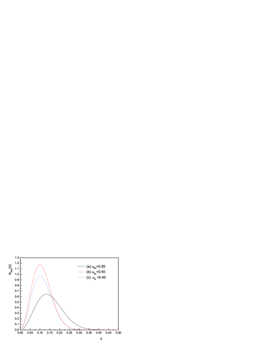
Figure 1: $B_{(s)}$ distribution amplitude as a function of light quark momentum fraction $x$ (The wave function comes to zero when $x\in\{0.5,1.0\}$ so we don’t show it here)

In this paper, we study $B_{s}\to\rho(\omega)K^{*}$ decays in the PQCD approach. Hopefully the branching ratio is not too small and can be detected by the TEVATRON or LHCb experiments, then it may allow us to determine the $B_{s}$ distribution amplitude and SU(3) breaking effects with much more precision. Moreover, we can also constrain $\alpha$ with fewer pollution from this channel.

2 Calculation and Numerical analysis

We use the effective Hamiltonian for the process $B_{s}\to\rho(\omega)K^{*}$ given by [22]

$${\cal H}_{eff}=\frac{G_{F}}{\sqrt{2}}\left\{V_{u}\left[C_{1}(\mu)O_{1}(\mu)+C_{2}(\mu)O_{2}(\mu)\right]-V_{t}\sum_{i=3}^{10}C_{i}(\mu)O_{i}^{(q)}(\mu)\right\},$$ (3)

where $V_{u}=V_{ud}^{*}V_{ub}$, $V_{t}=V_{td}^{*}V_{tb}$, $C_{i}(\mu)$ are the Wilson coefficients, and the operators are

$$O_{1}=(\bar{d}_{i}q_{j})_{V-A}(\bar{q}_{j}b_{i})_{V-A},\,O_{2}=(\bar{d}_{i}q_{i})_{V-A}(\bar{q}_{j}b_{j})_{V-A},$$

$$O_{3}=(\bar{d}_{i}b_{i})_{V-A}\sum\limits_{q}(\bar{q}_{j}q_{j})_{V-A},\,O_{4}=(\bar{d}_{i}b_{j})_{V-A}\sum\limits_{q}(\bar{q}_{j}q_{i})_{V-A},$$

$$O_{5}=(\bar{d}_{i}b_{i})_{V-A}\sum\limits_{q}(\bar{q}_{j}q_{j})_{V+A},\,O_{6}=(\bar{d}_{i}b_{j})_{V-A}\sum\limits_{q}(\bar{q}_{j}q_{i})_{V-A},$$

$$O_{7}=\frac{3}{2}(\bar{d}_{i}b_{i})_{V-A}\sum\limits_{q}e_{q}(\bar{q}_{j}q_{j})_{V+A},\,O_{8}=\frac{3}{2}(\bar{d}_{i}b_{j})_{V-A}\sum\limits_{q}e_{q}(\bar{q}_{j}q_{i})_{V+A},$$

$$O_{9}=\frac{3}{2}(\bar{d}_{i}b_{i})_{V-A}\sum\limits_{q}e_{q}(\bar{q}_{j}q_{j})_{V-A},\,O_{10}=\frac{3}{2}(\bar{d}_{i}b_{j})_{V-A}\sum\limits_{q}e_{q}(\bar{q}_{j}q_{i})_{V-A}.$$ (4)

Here i and j stand for $SU(3)$ color indices.

The decay width for these channels is :

$$\Gamma=\frac{G_{F}^{2}|{\bf p}|}{16\pi M_{B}^{2}}\sum\limits_{\sigma=L,T}{\cal M}^{\sigma{\dagger}}{\cal M}^{\sigma}$$ (5)

where ${\bf p}$ is the 3-momentum of the final state mesons, $|{\bf p}|=\frac{M_{B}}{2}(1-r^{2}_{K^{*}}-r^{2}_{\rho(\omega)})$, and $r_{K^{*}(\rho,\omega)}=m_{K^{*}(\rho,\omega)}/m_{B_{s}}$. ${\cal M}^{\sigma}$ is the decay amplitude , which will be calculated later in PQCD approach. The subscript $\sigma$ denotes the helicity states of the two vector mesons with the longitudinal (transverse) components L(T). According to Lorentz structure analysis, the amplitude can be decomposed into:

$${\cal M}^{\sigma}=M_{B_{s}}^{2}{\cal M}_{L}+M_{B_{s}}^{2}{\cal M}_{N}\epsilon^{\ast}_{2}(\sigma=T)\cdot\epsilon^{\ast}_{3}(\sigma=T)+i{\cal M}_{T}\epsilon_{\mu\nu\rho\sigma}\epsilon_{2}^{\mu\ast}\epsilon_{3}^{\nu\ast}P_{2}^{\rho}P_{3}^{\sigma}.$$ (6)

We can define the longitudinal $H_{0}$, transverse $H_{\pm}$ helicity amplitudes

$$H_{0}=M^{2}_{B_{s}}{\cal M}_{L},\,\,H_{\pm}=M^{2}_{B_{s}}{\cal M}_{N}\mp M_{K^{*}}^{2}\sqrt{r^{\prime 2}-1}{\cal M}_{T},$$ (7)

where $r^{\prime}=\frac{P_{2}\cdot P_{3}}{M_{K^{*}}M_{\rho(\omega)}}$. They satisfy the relation

$$\sum\limits_{\sigma=L,R}{\cal M}^{\sigma{\dagger}}{\cal M}^{\sigma}=|H_{0}|^{2}+|H_{+}|^{2}+|H_{-}|^{2}.$$ (8)

The leading order diagrams in PQCD approach are shown in Fig.2. The amplitudes for $B_{s}\to\rho{K}^{\ast 0}$ and $\bar{B}_{s}\to\rho\bar{K}^{\ast 0}$are written as

$${\cal M}_{H} = V_{u}^{*}T_{H}-V_{t}^{*}P_{H},$$ (9)

$$\bar{\cal M}_{H} = V_{u}T_{H}-V_{t}P_{H},$$ (10)

respectively, where the subscript $H$ denote different helicity amplitudes $L,N$ and $T$, and $T_{H}$ and $P_{H}$ are the amplitudes from tree and penguin diagrams respectively. The detailed formulae of $T_{H}$ and $P_{H}$ are similar to those in $B\to K^{*}K^{*}$ [23] and $B\to\phi K^{*}$ [15], so we will not show them here.

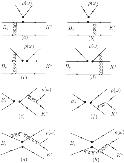
Figure 2: Leading order Feynman diagrams for $B_{s}\rightarrow\rho(\omega)K^{*}$

The parameters used in our calculations are: the Fermi coupling constant $G_{F}=1.16639\times 10^{-5}GeV^{-2}$, the meson masses $M_{B_{s}}=5.37GeV,\ M_{K^{*}}=0.89GeV,\ M_{\rho(\omega)}=0.77GeV$ [24], the decay constants $f_{K^{*}}=0.217GeV,\ f_{K^{*}}^{T}=0.16GeV,\ f_{\rho}=0.205GeV,\ f_{\rho}^{T}=0.155GeV,\ f_{\omega}=0.195GeV,\ f_{\omega}^{T}=0.14GeV$ [25], the central value of the CKM matrix elements $\alpha=95^{\circ}$, $|V_{td}|=0.0075,\ |V_{tb}|=0.9992,\ |V_{ud}|=0.9745$ [24], $|V_{ub}|=0.0047$ [26] and the $B_{s}$ meson lifetime $\tau_{B_{s}}=1.461ps$ [24].

Table 1: Branching ratio, polarization fraction and direct CP asymmetry dependence on $\omega_{B_{s}}$

Channel	$\omega_{B_{s}}$	BR$(10^{-6})$	$|A_{0}|^{2}$	$|A_{\|}|^{2}$	$|A_{\perp}|^{2}$	$A^{dir}_{CP}$
	0.50	0.41	0.38	0.28	0.34	-0.63
$B_{s}(\bar{B}_{s})\to\rho^{0}\bar{K}^{\ast 0}(K^{*0})$	0.55	0.34	0.41	0.27	0.32	-0.67
	0.60	0.30	0.44	0.26	0.30	-0.70
	0.50	0.56	0.33	0.31	0.36	0.56
$B_{s}(\bar{B}_{s})\to\omega\bar{K}^{\ast 0}(K^{*0})$	0.55	0.47	0.35	0.30	0.35	0.58
	0.60	0.40	0.37	0.29	0.34	0.60
	0.50	16	0.92	0.04	0.04	0.10
$B_{s}(\bar{B}_{s})\to\rho^{\pm}K^{*\mp}$	0.55	12	0.92	0.04	0.04	0.12
	0.60	10	0.92	0.04	0.04	0.13

As we mentioned before, the decay $B_{s}\to\rho(\omega)K^{*}$ can be used to determine the $B_{s}$ meson wave function parameter $\omega_{B_{s}}$, or $\omega_{B_{s}}$ can influence our predictions of $B_{s}\to\rho(\omega)K^{*}$ decay. So we show the results in Table 1 according to 3 different values of $\omega_{B_{s}}$. From the table we can easily find out the averaged branching ratio for $B_{s}(\bar{B}_{s})\to\rho^{\pm}K^{*\mp}$ is much larger than the other two, for $B_{s}(\bar{B}_{s})\to\rho^{\pm}K^{*\mp}$ involve large Wilson coefficient $C(2)+C(1)/3$ for the factorizable part while the other two ($B_{s}(\bar{B}_{s})\to\rho^{0}\bar{K}^{*0}(K^{*0})$ and $B_{s}(\bar{B}_{s})\to\omega\bar{K}^{*0}(K^{*0})$) involve a much smaller Wilson coefficient $C(1)+C(2)/3$ (color-suppressed) for the factorizable part of the emission diagram. As a result the first one is tree dominated and has a large branching ratio and small direct CP asymmetry. While referring to the other two, the contributions from penguin and tree diagrams are at the same order ($Z_{H}\simeq 0.5\sim 1.5$), hence we can expect a large direct CP asymmetry from eqs.(13).

The polarization fraction difference of these channels are also due to that the main contribution of each channel comes from different topology. $B_{s}(\bar{B}_{s})\to\rho^{\pm}K^{*\mp}$ is tree dominated. The main contribution comes from the factorizable part of the emission diagram, where transverse polarization amplitude is suppressed by a factor $r_{\rho}^{2}\simeq(0.77/5.37)^{2}$ (see formulas in [23]), so the longitudinal polarization dominates and contributes more than $90\%$ of the total branching ratio. But in $B_{s}(\bar{B}_{s})\to\rho^{0}\bar{K}^{*0}(K^{*0})$ and $B_{s}(\bar{B}_{s})\to\omega\bar{K}^{*0}(K^{*0})$ decays, tree emission (factorizable) diagram contribution is suppressed due to the cancellation of Wilson coefficients $C_{1}+C_{2}/3$. The left dominant contribution is the non-factorizable diagrams of tree operators and penguin diagrams. both of these contributions equally contribute to longitudinal and transverse polarizations. The transverse polarization is not suppressed in those cases, therefore numerically we get a small longitudinal fraction of about 0.4. This similar situation is also found in $B\to\rho\rho(\omega)$ decays [27], which are related by SU(3) symmetry to our $B_{s}\to\rho K^{*}$ decays.

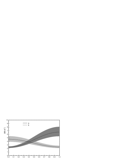
Figure 3: Average branching ratios when $\omega_{B_{s}}$ was set from 0.50 to 0.60: $(a)B_{s}(\bar{B}_{s})\rightarrow\rho^{0}\bar{K}^{*0}(K^{*0})$; (b) $B_{s}(\bar{B}_{s})\rightarrow\omega\bar{K}^{*0}(K^{*0})$

To extract the CP violation parameters and dependence on CKM phase angle $\alpha$ of these decays, we rewrite the helicity amplitudes in (9,10) as the functions of $\alpha$:

$${\cal M}_{H}^{+} = V_{u}^{*}T_{H}-V_{t}^{*}P_{H}$$ (11)

$$= V_{u}^{*}T_{H}(1+Z_{H}e^{i(\alpha+{\delta}_{H})})$$

$${\cal M}_{H}^{-} = V_{u}T_{H}-V_{t}P_{H}$$ (12)

$$= V_{u}T_{H}(1+Z_{H}e^{i(-\alpha+{\delta}_{H})})$$

where $Z_{H}=|V_{t}^{*}/V_{u}^{*}||P_{H}/T_{H}|$, and $\delta$ is the relative strong phase between tree ($T$) and penguin ($P$) diagrams. Here in PQCD approach, the strong phase comes from the nonfactorizable diagrams and annihilation diagrams. This is different from Beneke-Buchalla-Neubert-Sachrajda [7] approach. In that approach, annihilation diagrams are not taken into account, strong phases mainly come from the so-called Bander-Silverman-Soni mechanism [28]. As shown in [5], these effects are in fact next-to-leading-order ($\alpha_{s}$ suppressed) elements and can be neglected in PQCD approach. We give the averaged branching ratios of $B_{s}(\bar{B}_{s})\to\rho^{0}K^{*0}(\bar{K}^{*0})$ and $B_{s}(\bar{B}_{s})\to\omega K^{*0}(\bar{K}^{*0})$ as a function of $\alpha$ in Fig.3, and the averaged branching ratios of $B^{0}(\bar{B}^{0})\to\rho^{\pm}K^{*\mp}$ in Fig.4.

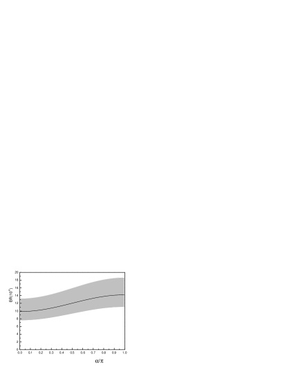
Figure 4: Average branching ratios for $B_{s}(\bar{B}_{s})\rightarrow\rho^{\pm}K^{*\mp}$as a function of $\alpha$ when $\omega_{B_{s}}$ was set from 0.50 to 0.60

Using Eqs.(11,12), the direct CP violating parameter is

$$A^{dir}_{CP} = \frac{{|M|}^{2}-{|\bar{M}|}^{2}}{{|M|}^{2}+{|\bar{M}|}^{2}}$$ (13)

$$= \frac{-2sin\alpha\left(T_{L}^{2}sin\delta_{L}+2T_{N}^{2}sin\delta_{N}+2T_{T}^{2}sin\delta_{T}\right)}{T_{L}^{2}(1+Z_{L}^{2}+2Z_{L}cos\alpha cos\delta_{L})+2\sum_{i=N,T}T_{i}^{2}\left(1+Z_{i}^{2}+2Z_{i}cos\alpha cos\delta_{i}\right)}.$$

Notice the CP asymmetry for these channels are sensitive to CKM angle $\alpha$, we show the direct CP asymmetry as a function of $\alpha$ in Fig.5. It is easy to see that the $B_{s}\to\rho^{0}K^{*0}$ and $\omega K^{*0}$ have large direct CP asymmetries up to 50%, with a relative minus sign. On the other hand, the $B_{s}\to\rho^{\pm}K^{*\mp}$ decay has small direct CP asymmetry due to only one large tree contribution in this decay. The uncertainty shown at this table is only from the $B_{s}$ meson wave function parameter dependence. In fact, since CP asymmetry is sensitive to many parameters, the line should be more broadened by uncertainties. The mixing induced CP asymmetry is complicated and requires angular distribution study, similar study may be found in [29].

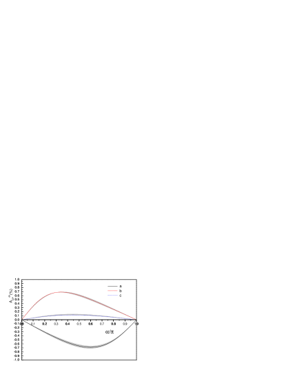
Figure 5: Direct CP asymmetry $A_{CP}^{dir}$ as a function of $\alpha$: (a) $\ B_{s}(\bar{B}_{s})\rightarrow\rho^{0}\bar{K}^{*0}(K^{*0})$ (lower line); (b) $B_{s}(\bar{B}_{s})\rightarrow\omega\bar{K}^{*0}(K^{*0})$ (upper line); (c) $B_{s}(\bar{B}_{s})\rightarrow\rho^{\pm}K^{*\mp}$ (middle line).

At last, if we compare our predictions with those of naive factorization [30]

$$BR(B_{s}(\bar{B}_{s})\to\rho^{0}\bar{K}^{\ast 0}(K^{*0}))=5.5\times 10^{-7},$$ (14)

$$BR(B_{s}(\bar{B}_{s})\to\omega\bar{K}^{*0}(K^{*0}))=6.0\times 10^{-7},$$ (15)

$$BR(B_{s}(\bar{B}_{s})\to\rho^{\pm}K^{*\mp})=1.7\times 10^{-5},$$ (16)

and ones of QCDF [31]

$$BR(B_{s}(\bar{B}_{s})\to\rho^{0}\bar{K}^{\ast 0}(K^{*0}))=5.3\times 10^{-7},$$ (17)

$$BR(B_{s}(\bar{B}_{s})\to\omega\bar{K}^{*0}(K^{*0}))=3.1\times 10^{-7},$$ (18)

$$BR(B_{s}(\bar{B}_{s})\to\rho^{\pm}K^{*\mp})=1.8\times 10^{-5}.$$ (19)

We can see that they are consistent. It should be noticed that the branching ratios in FA and QCDF strongly depend on form factors. While in PQCD, the branching ratios and form factors depend on wave functions, especially the $B_{s}$ meson wave function. Nowadays, very few $B_{s}$ meson decays have been measured, so we can only give rough constraints on the parameters from other channel and permit large errors. More experimental data can help to constrain the form factors and wave functions, then we can give more precise predictions and the different methods can be tested by the experiments. Although similar results are got by different methods for branching ratios, the polarization fractions are quite different. The QCDF and naive factorization give only several percent transverse polarization for all three decay modes [31], while Table 1 shows large transverse contribution for $B_{s}\to\rho^{0}(\omega)K^{*0}$ decays in our PQCD approach. The direct CP asymmetry are not given in ref.[31], but they probably also differ from PQCD approach as it happened in $B\to\pi\pi$ and $K\pi$ case [32].

The numerical results shown here are only leading order ones. For the tree dominated channel $B_{s}\to\rho^{\pm}K^{*\mp}$, the leading order diagrams should give the main contribution. But for the other two decays, with a branching ratio as small as $10^{-7}$, the next-to-leading order and power suppressed contributions should not be negligible, the results may suffer from large corrections when the next to leading order corrections are included [33].

Current experiments [24] only give the upper limit for the decay

$$BR(B_{s}\to\rho^{0}\bar{K}^{\ast 0})<7.6\times 10^{-4}.$$ (20)

More data are needed to test our calculations.

3 Summary

In this paper we calculate the branching ratios, polarization fraction and CP asymmetries of $B_{s}\to\rho(\omega)K^{*}$ modes using PQCD theorem in SM. We perform all leading order diagrams to next to leading twist wave functions. We also study the dependence of their averaged branching ratios and the CP asymmetry on the CKM angle $\alpha$. At last we compare our predictions with values from other approaches.

Appendix A wave function

For longitudinal polarized $K^{*}$ meson, the wave function is written as

$$\frac{1}{\sqrt{2N_{c}}}[M_{K^{*}}\not\!\epsilon_{2L}\phi_{K^{*}}(x)+\not\!\epsilon_{2L}\not\!P_{2}\phi_{K^{*}}^{t}(x)+M_{\phi}I\phi^{s}_{K^{*}}(x)],$$ (21)

and the wave function for transverse polarized $K^{*}$ meson reads

$$\frac{1}{\sqrt{2N_{c}}}[M_{K^{*}}\not\!\epsilon_{2T}\phi^{v}_{K^{*}}(x)+\not\!\epsilon_{2T}\not\!P_{2}\phi_{K^{*}}^{T}(x)+\frac{M_{K^{*}}}{P_{2}\cdot n_{-}}i\epsilon_{\mu\nu\rho\sigma}\gamma_{5}\gamma^{\mu}\epsilon_{2T}^{\nu}P_{2}^{\rho}n_{-}^{\sigma}\phi^{a}_{K^{*}}(x)].$$ (22)

The $K^{*}$ meson distribution amplitudes up to twist-3 are given by ref.[34] with QCD sum rules.

$$\phi_{K^{*}}(x)=\frac{3f_{K^{*}}}{\sqrt{2N_{c}}}x(1-x)[1+0.57(1-2x)+0.07C_{2}^{3/2}(1-2x)],$$ (23)

$$\phi^{t}_{K^{*}}(x)=\frac{f_{K^{*}}^{T}}{2\sqrt{2N_{c}}}\left\{0.3(1-2x)[3(1-2x)^{2}+10(1-2x)-1]+1.68C_{4}^{1/2}(1-2x)\right.$$

$$\left.\ \ \ \ \ \ \ \ \ \ \ \ +0.06(1-2x)^{2}[5(1-2x)^{2}-3]+0.36\left\{1-2(1-2x)[1+\ln(1-x)]\right\}\right\},$$ (24)

$$\phi^{s}_{K^{*}}(x)=\frac{f_{K^{*}}^{T}}{2\sqrt{2N_{c}}}\left\{3(1-2x)\left[1+0..2(1-2x)+0.6(10x^{2}-10x+1)\right]\right.$$

$$\left.\ \ \ \ \ \ \ \ \ \ \ \ -0.12x(1-x)+0.36[1-6x-2\ln{(1-x)}]\right\},$$ (25)

$$\phi^{T}_{K^{*}}(x)=\frac{3f_{K^{*}}^{T}}{\sqrt{2N_{c}}}x(1-x)[1+0.6(1-2x)+0.04C_{2}^{3/2}(1-2x)],$$ (26)

$$\phi^{v}_{K^{*}}(x)=\frac{f_{K^{*}}^{T}}{2\sqrt{2N_{c}}}\left\{\frac{3}{4}[1+(1-2x)^{2}+0.44(1-2x)^{3}]\right.$$

$$\left.\ \ \ \ \ \ \ \ \ \ \ \ +0.4C_{2}^{1/2}(1-2x)+0.88C_{4}^{1/2}(1-2x)+0.48[2x+\ln(1-x)]\right\},$$ (27)

$$\phi^{a}_{K^{*}}(x)=\frac{f_{K^{*}}^{T}}{4\sqrt{2N_{c}}}\left\{3(1-2x)[1+0.19(1-2x)+0.81(10x^{2}-10x+1)]\right.$$

$$\left.\ \ \ \ \ \ \ \ \ \ \ \ -1.14x(1-x)+0.48[1-6x-2\ln(1-x)]\right\},$$ (28)

where the Gegenbauer polynomials are

$$C_{2}^{\frac{1}{2}}(\xi)=\frac{1}{2}(3\xi^{2}-1),$$ (29)

$$C_{4}^{\frac{1}{2}}(\xi)=\frac{1}{8}(35\xi^{4}-30\xi^{2}+3),$$ (30)

$$C_{2}^{\frac{3}{2}}(\xi)=\frac{3}{2}(5\xi^{2}-1).$$ (31)

For $\rho$ and $\omega$ meson, we employ $\rho^{0}=\frac{1}{\sqrt{2}}(u\bar{u}-d\bar{d})$ and $\omega=\frac{1}{\sqrt{2}}(u\bar{u}+d\bar{d})$. Their Lorentz structures are similar to $K^{*}$ meson, the distribution amplitudes are the same for $\rho$ and $\omega$ and given as [34]:

$$\phi_{\rho}(x) = \frac{3f_{\rho}}{\sqrt{2N_{c}}}x(1-x)\left[1+0.18C_{2}^{3/2}(1-2x)\right]\;,$$ (32)

$$\phi_{\rho}^{t}(x) = \frac{f^{T}_{\rho}}{2\sqrt{2N_{c}}}\left\{3(1-2x)^{2}+0.3(1-2x)^{2}[5(1-2x)^{2}-3]\right.$$ (33)

$$\left.+0.21[3-30(1-2x)^{2}+35(1-2x)^{4}]\right\}\;,$$

$$\phi_{\rho}^{s}(x) = \frac{3f_{\rho}^{T}}{2\sqrt{2N_{c}}}(1-2x)\left[1+0.76(10x^{2}-10x+1)\right]\;,$$ (34)

$$\phi_{\rho}^{T}(x) = \frac{3f_{\rho}^{T}}{\sqrt{2N_{c}}}x(1-x)\left[1+0.2C_{2}^{3/2}(1-2x)\right]\;,$$ (35)

$$\phi_{\rho}^{v}(x) = \frac{f_{\rho}}{2\sqrt{2N_{c}}}\bigg{\{}\frac{3}{4}[1+(1-2x)^{2}]+0.24[3(1-2x)^{2}-1]$$ (36)

$$+0.12[3-30(1-2x)^{2}+35(1-2x)^{4}]\bigg{\}}\;,$$

$$\phi_{\rho}^{a}(x) = \frac{3f_{\rho}}{4\sqrt{2N_{c}}}(1-2x)\left[1+0.93(10x^{2}-10x+1)\right]\;.$$ (37)

References

- [1] M. Wirbel, B. Stech, M. Bauer, Z. Phys. C29, 637 (1985); M. Bauer, B. Stech, M. Wirbel, Z. Phys. C34, 103 (1987); L.-L. Chau, H.-Y. Cheng, W.K. Sze, H. Yao, B. Tseng, Phys. Rev. D43, 2176 (1991).
- [2] A. Ali, G. Kramer and C.D. Lü, Phys. Rev. D 58, 094009; C.D. Lü, Nucl. Phys. Proc. Suppl. 74; Y.H. Cheng, et al, Phys. Rev. D 60, 094014 (1999).
- [3] G.P. Leapage and S.J. Brodsky, Phys. Rev. D 22, 2157 (1980); S.J. Brodsky, G.P. Lepage, P.B. Mackenzie, Phys. Rev. D 28, 228 (1983).
- [4] H-n. Li and H.L. Yu, Phys. Rev. Lett. 74, 4388 (1995); Phys. Lett. B 353, 301 (1995); Phys. Rev. D 53, 2480 (1996).
- [5] Y.Y. Keum, H-n. Li, and A.I. Sanda, Phys. Lett. B 504, 6 (2001); Phys. Rev. D 63, 054008 (2001); Y.Y. Keum and H-n Li, Phys. Rev. D 63, 074006 (2001).
- [6] C. D. Lü, K. Ukai, and M. Z. Yang, Phys. Rev. D 63, 074009 (2001); C. D. Lü and M.Z. Yang, Eur. Phys. J. C 23, 275 (2002).
- [7] M. Beneke, G. Buchalla, M. Neubert and C.T. Sachrajda, Phys. Rev. Lett. 83, 1914 (1999); Nucl. Phys. B 591, 313 (2000).
- [8] M. Beneke, G. Buchalla, M. Neubert and C.T. Sachrajda, Nucl. Phys. B 606, 245 (2001), Nucl. Phys. B 675, 333-415 (2003).
- [9] C.W. Bauer, S. Fleming, and M. Luke, Phys. Rev. D 63, 014006 (2001), C.W. Bauer, S. Fleming, D. Pirjol, and I.W. Stewart, Phys. Rev. D 63, 114020 (2001); C.W. Bauer and I.W. Stewart, Phys. Lett. B 516, 134 (2001), Phys. Rev. D 65, 054022 (2002).
- [10] S. Catani, M. Ciafaloni and F. Hautmann, Phys. Lett. B 242, 97 (1990); Nucl. Phys. B 366, 135 (1991).
- [11] J.C. Collins and R.K. Ellis, Nucl. Phys. B 360, 3 (1991).
- [12] E.M. Levin, M.G. Ryskin, Yu.M. Shabelskii, and A.G. Shuvaev, Sov.J. Nucl.Phys. 53, 657 (1991).
- [13] H-n. Li, Phys. Rev. D66, 094010 (2002); H-n. Li, K. Ukai, Phys. Lett. B 555, 197 (2003).
- [14] H-n. Li and M. Nagashima, Phys. Rev. D67 (2003) 034001
- [15] C.H. Chen, H-n. Li, Phys.Rev. D 66 (2002) 054013.
- [16] Y.Y. Keum, T. Kurimoto, H-n. Li, C.D. Lu, A.I. Sanda, Phys. Rev. D69 (2004) 094018; C.D. Lü, M.Z. Yang, Eur. Phys. J. C23 (2002) 275-287; C.D. Lü, Y.L. Shen and J. Zhu, Eur. Phys. J. C41, 311-317 (2005).
- [17] A. Warburton et al,CDF Collaboration, Int. J. Mod. Phys. A20, 3554-3558 (2005).
- [18] X.Q. Yu, Y. Li, C.D. Lü, Phys. Rev. D71, 074026 (2005).
- [19] M. Rescigno, hep-ex/0410063, CDF Collaboration, D. Acosta et al, Phys. Rev. Lett. 95, 031801 (2005).
- [20] J.F. Cheng, C.D. Lü, Y.L. Shen and J. Zhu, In preparation.
- [21] J.-X. Chen, Z.-Y. Hou, Y. Li, C.-D. Lu, e-Print Archive: hep-ph/0509093.
- [22] G. Buchalla, A. J. Buras and M. E. Lautenbacher, Rev. Mod. Phys. 68, 1125 (1996).
- [23] J. Zhu, Y.L. Shen and C.D. Lü, Phys. Rev. D72, 054015 (2005).
- [24] Particle Data Group, S. Eidelman et al., Phys. Lett. B 592, 1 (2004).
- [25] P. Ball and R. Zwicky, Phys. Rev. D71, 014029 (2005).
- [26] Heavy Flavor Averaging Group, hep-ex/0412073.
- [27] Y. Li, C.D. Lü, e-Print Archive: hep-ph/0508032.
- [28] M. Bander, D. Silverman, and A. Soni, Phys. Rev. Lett. 43, 242 (1979).
- [29] G. Kramer, W.F. Plamer, Phys. Rev. D 45, 193 (1992); C.S. Kim, Y.G. Kim, C.D. Lu, T. Morozumi, Phys. Rev. D 62, 034013 (2000).
- [30] H.Y. Chen, H.Y. Cheng, B. Tseng, Phys. Rev. D 59, 074003 (1999).
- [31] X.Q. Li, G.R. Lu, and Y.D. Yang, Phys. Rev. D 68 (2003) 114015; Erratum-ibid. D71, 019902 (2005).
- [32] B.H. Hong, C.-D. Lu, e-Print Archive: hep-ph/0505020
- [33] H.-n. Li, S. Mishima, A.I. Sanda, hep-ph/0508041.
- [34] P. Ball, V. M. Braun, Y. Koike, K. Tanaka, Nucl. phys. B 529, 323 (1998).