QCD Analytic Perturbation Theory. From integer powers to any power of the running coupling

A. P. Bakulev bakulev@theor.jinr.ru Bogoliubov Laboratory of Theoretical Physics, JINR, 141980 Dubna, Russia
   S. V. Mikhailov mikhs@theor.jinr.ru Bogoliubov Laboratory of Theoretical Physics, JINR, 141980 Dubna, Russia
   N. G. Stefanis stefanis@tp2.ruhr-uni-bochum.de Institut für Theoretische Physik II, Ruhr-Universität Bochum, D-44780 Bochum, Germany
Abstract

We propose a new generalized version of the QCD Analytic Perturbation Theory of Shirkov and Solovtsov for the computation of higher-order corrections in inclusive and exclusive processes. We construct non-power series expansions for the analytic images of the running coupling and its powers for any fractional (real) power and complete the linear space of these solutions by constructing the index derivative. Using the Laplace transformation in conjunction with dispersion relations, we are able to derive at the one-loop order closed-form expressions for the analytic images in terms of the Lerch function. At the two-loop order we provide approximate analytic images of products of powers of the running coupling and logarithms—typical in higher-order perturbative calculations and when including evolution effects. Moreover, we supply explicit expressions for the two-loop analytic coupling and the analytic images of its powers in terms of one-loop quantities that can strongly simplify two-loop calculations. We also show how to resum powers of the running coupling while maintaining analyticity, a procedure that captures the generic features of Sudakov resummation. The algorithmic rules to obtain analytic coupling expressions within the proposed Fractional Analytic Perturbation Theory from the standard QCD power-series expansion are supplied ready for phenomenological applications and numerical comparisons are given for illustration.

pacs:
11.15.Bt, 12.38.Bx, 12.38.Cy
preprint: RUB-TPII-06/05, JINR-E2-2005-156

I Introduction

A fundamental goal of perturbative QCD is to provide a microscopic description of hadronic short-distance phenomena that yields reliable predictions to be compared with experimental data of increasing precision. While singularities on the timelike axis in the complex Q2superscript𝑄2Q^{2} plane of hadronic observables are related to physical particles (or resonances), the appearance of singularities on the spacelike axis are unphysical and may violate causality. On the other hand, the expansion of hadronic quantities at large momentum transfer Q2superscript𝑄2Q^{2} can be safely calculated in terms of a power-series expansion in the running strong coupling αs(Q2)subscript𝛼𝑠superscript𝑄2\alpha_{s}(Q^{2}) by virtue of asymptotic freedom. But the one-loop running coupling contains at Q2=ΛQCD2superscript𝑄2superscriptsubscriptΛQCD2Q^{2}=\Lambda_{\rm QCD}^{2} (ΛQCDΛsubscriptΛQCDΛ\Lambda_{\rm QCD}\equiv\Lambda in the following) a ghost singularity—the Landau pole—that spoils its analyticity structure. To restore analyticity and ensure causality in the whole Q2superscript𝑄2Q^{2} plane, this pole has to be removed. With most available experimental data on several exclusive processes being at rather low Q2superscript𝑄2Q^{2} values, the Landau-singularity problem is not only of academic interest, but affects significantly perturbative predictions in the low-to-medium Q2superscript𝑄2Q^{2} domain. The reason is that—lacking all-order perturbative expressions—one has to resort to a renormalization-scheme choice that makes the uncalculated higher-order corrections negligible and adopt a renormalization scale that reflects the typical parton virtualities in the considered process. The latter procedure, however, may result into a scale in the region of only a few ΛΛ\Lambda, where the application of perturbation theory for the conventional running coupling without infrared (IR) protection against the Landau pole becomes inapplicable—a prominent example being the Brodsky–Lepage–Mackenzie scale-setting procedure BLM83 . Different strategies have been suggested over the years as how to minimize the dependence on the renormalization scheme and scale setting—unavoidable in any perturbative calculation beyond the leading order—and obtain reliable and stable results in the low-momentum regime (see, for example, Ref. BPSS04 for a recent extensive discussion of these issues in terms of the electromagnetic pion form factor and references cited therein).

In a series of papers during the last few years Shirkov and Solovtsov (SS) SS97 ; Shi98 ; SS99 ; Shi01 ; SS01 have developed an approach which enables the removal of the Landau singularity without introducing extraneous IR regulators, like an effective gluon mass PP79 ; Cor82 ; GHN93 ; MS92 ; MaSt93 . The analyticity of the coupling in the spacelike region is achieved by a nonperturbative, power-behaved term that contains no other scale than ΛΛ\Lambda and leaves the ultraviolet (UV) behavior of the running coupling unchanged. At zero-momentum transfer the Shirkov–Solovtsov coupling assumes a universal value that depends solely on renormalization-group constants. Using dispersion relations, this scheme was both generalized (in approximate form) to higher-loop orders and also extended to the timelike regime DVS00unp ; Shi00b ; Shi04 ; SS98 ; BRS00 ; Shi01 ; SS01 ; Gru97 ; GGK98 ; Mag99 ; KM01 ; KM03 ; Mag03u , encompassing previous incomplete attempts Rad96 ; KP82 in this direction, and amounting to the theoretical framework of Analytic Perturbation Theory (APT). There have been a number of parallel developments by various authors during the past several years to avoid the Landau pole using different “analytization” techniques, prime examples being Refs. KP82 ; Rad96 ; CS93 ; BB95 ; BBB95 ; DMW96 ; CMNT96 ; Gru97 ; GGK98 ; Magn00 ; BRS00 ; Gar01 ; Nes03 ; NP04 ; ANP05 .

Two other major challenges, connected with—first—the implementation of the Shirkov–Solovtsov “analytization” to three-point functions beyond the leading order of perturbation theory and—second—the extension to non-integer powers of the coupling, remained open, or at least partially open. Indeed, in the first case, extensive analyses SSK99 ; SSK00 ; BPSS04 have shown that the “analytization” principle has to be generalized to accommodate a second scale, serving as a factorization scale, or in order to include evolution effects comprising typical logarithms to some fractional power. Technically speaking, this means to extend the assertion of analyticity from the level of the coupling (and its powers) to the level of the whole reaction amplitude. This requirement was formalized by Karanikas and Stefanis (KS) in KS01 ; Ste02 in an attempt to calculate power corrections to the pion form factor and the Drell–Yan process. The systematic development of a perturbative expansion in terms of fractional powers of the coupling—the second major challenge—is the goal of the present investigation, the main focus being placed on the methodology towards improving perturbative higher-order calculations in QCD. This goal has been accomplished and will be described in this paper. A specific application of the KS “analytization” principle to the pion’s electromagnetic form factor at NLO accuracy is given in fully worked out detail in BKS05 . Other applications will follow in future publications in conjunction with the inclusion of heavy-flavor thresholds and the extension to the timelike regime.

The paper is organized as follows. In Sec. II we first review the key features of the original Analytic Perturbation Theory of Shirkov and Solovtsov, highlighting those properties pertaining to the generalization of the approach to fractional powers of the coupling. The actual extension of the approach to fractional—in fact, real—powers of the coupling is performed in Sec. III. This section describes in three subsections the new “analytization” technique, based on the Laplace transform, the verification of the analytic properties of the obtained results, and the way to include products of powers of the coupling with powers of logarithms. Moreover, we provide here approximate expressions for two-loop quantities in terms of one-loop analytic-coupling images and their index derivatives that can be extremely useful in practical calculations. Section IV is devoted to the validation of the developed theoretical framework of the Fractional Analytic Perturbation Theory (FAPT) and includes a table where we collect the algorithmic rules to connect the new analytic framework to the standard QCD perturbative power-series expansion. Our conclusions are drawn in Sec. V, while important technical details are presented in three appendices.

II Original Analytic Perturbation Theory

In the analytic perturbation-theory approach of Shirkov and Solovtsov, the power-series expansion in the running coupling is given up in favor of a non-power series (functional) expansion. This can be written generically in terms of numerical coefficients dmsubscript𝑑𝑚d_{m} in the following way MS97 ; Shi98

mdma(l)m(Q2)mdm𝒜m(l)(Q2),subscript𝑚subscript𝑑𝑚superscriptsubscript𝑎𝑙𝑚superscript𝑄2subscript𝑚subscript𝑑𝑚subscriptsuperscript𝒜𝑙𝑚superscript𝑄2\displaystyle\sum\limits_{m}d_{m}a_{(l)}^{m}(Q^{2})\Rightarrow\sum\limits_{m}d_{m}{\cal A}^{(l)}_{m}(Q^{2})\,, (1)

where the “normalized” coupling a=b0αs/(4π)𝑎subscript𝑏0subscript𝛼𝑠4𝜋a=b_{0}\alpha_{s}/(4\pi) (b0subscript𝑏0b_{0} is the first coefficient of the QCD β𝛽\beta-function—see Appendix B) has been introduced instead of αssubscript𝛼𝑠\alpha_{s} in order to simplify intermediate calculations and because then the analytic coupling 𝒜1subscript𝒜1\mathcal{A}_{1} is bounded from above by unity Shi98 . In the above expression, the superscript m𝑚m on a(l)msuperscriptsubscript𝑎𝑙𝑚a_{(l)}^{m} appears on the left-hand side (LHS) as a power, whereas on the right-hand side (RHS) the subscript m𝑚m on 𝒜m(l)subscriptsuperscript𝒜𝑙𝑚{\cal A}^{(l)}_{m} denotes the index of the functional expansion;111In the following, a calligraphic notation is used to denote analytic images. (l)𝑙(l) denotes the loop order. For the sake of simplicity, we will avoid to indicate the loop-order index explicitly because we mostly work in the one-loop approximation; deviations, if needed, will be labelled by appropriate superscripts or subscripts in parentheses, like in Eq. (1). The conversion to analytic images of the coupling is achieved in terms of the functions

𝒜m(l)(Q2)[a(l)m(Q2)]ansubscriptsuperscript𝒜𝑙𝑚superscript𝑄2subscriptdelimited-[]superscriptsubscript𝑎𝑙𝑚superscript𝑄2an\displaystyle{\cal A}^{(l)}_{m}(Q^{2})\equiv\left[a_{(l)}^{m}(Q^{2})\right]_{\text{an}} (2)

according to the general prescription

[f(Q2)]an=1π0Im[f(σ)]σ+Q2iϵ𝑑σ.subscriptdelimited-[]𝑓superscript𝑄2an1𝜋superscriptsubscript0Imdelimited-[]𝑓𝜎𝜎superscript𝑄2𝑖italic-ϵdifferential-d𝜎\displaystyle\left[f(Q^{2})\right]_{\text{an}}=\frac{1}{\pi}\int_{0}^{\infty}\!\frac{\textbf{Im}\,\big{[}f(-\sigma)\big{]}}{\sigma+Q^{2}-i\epsilon}\,d\sigma\,. (3)

For the one-loop running coupling

a=1ln(Q2/Λ2),𝑎1superscript𝑄2superscriptΛ2\displaystyle a=\frac{1}{\ln(Q^{2}/\Lambda^{2})}\,, (4)

we have

𝒜1(Q2)[a(Q2)]an=1ln(Q2/Λ2)1Q2/Λ21subscript𝒜1superscript𝑄2subscriptdelimited-[]𝑎superscript𝑄2an1superscript𝑄2superscriptΛ21superscript𝑄2superscriptΛ21\displaystyle{\cal A}_{1}(Q^{2})\equiv\left[a(Q^{2})\right]_{\text{an}}=\frac{1}{\ln(Q^{2}/\Lambda^{2})}-\frac{1}{Q^{2}/\Lambda^{2}-1} (5)

and 𝒜1(1)(0)=1superscriptsubscript𝒜1101{\cal A}_{1}^{(1)}(0)=1. Employing the variable L=ln(Q2/Λ2)𝐿superscript𝑄2superscriptΛ2L=\ln(Q^{2}/\Lambda^{2}), which naturally appears in perturbative QCD (pQCD) calculations, we can recast a𝑎a and 𝒜𝒜{\cal A} in terms of L𝐿L to obtain

a1(L)=1L,𝒜1(L)=1L1eL1.formulae-sequencesuperscript𝑎1𝐿1𝐿subscript𝒜1𝐿1𝐿1superscript𝑒𝐿1\displaystyle a^{1}(L)=\frac{1}{L},\quad{\cal A}_{1}(L)=\frac{1}{L}-\frac{1}{e^{L}-1}\,. (6)

In this context, amplitudes (depending on a single scale Q2superscript𝑄2Q^{2}) perturbatively expanded in terms of the powers of the running coupling map on a non-power series expansion Shi98 ; MS97 :

F(a)=nfnan(L)(L)=nfn𝒜n(L),𝐹𝑎subscript𝑛subscript𝑓𝑛superscript𝑎𝑛𝐿𝐿subscript𝑛subscript𝑓𝑛subscript𝒜𝑛𝐿\displaystyle F(a)=\sum_{n}f_{n}a^{n}(L)\Rightarrow{\cal F}(L)=\sum_{n}f_{n}\,{\cal A}_{n}(L)\,, (7)

where fnsubscript𝑓𝑛f_{n} are numbers in minimal subtraction renormalization schemes. By construction, the set {𝒜n}subscript𝒜𝑛\{{\cal A}_{n}\} constitutes a linear space, which, however, is not equipped with the multiplication operation of its elements. Therefore, the product 𝒜n𝒜msubscript𝒜𝑛subscript𝒜𝑚{\cal A}_{n}\cdot{\cal A}_{m} has no rigorous meaning here. The standard algebra is recovered only for the main asymptotic contribution (cf. Eq. (6)) at L𝐿L\to\infty, when {𝒜n}{an}subscript𝒜𝑛superscript𝑎𝑛\{{\cal A}_{n}\}\to\{a^{n}\} SS97 ; Shi98 ; SS99 .

Let us now turn to the properties of this map and of the space {𝒜n}subscript𝒜𝑛\{{\cal A}_{n}\}. There are several points to note about them.

  1. 1.

    The map should have the property of isomorphism, i. e., it should conserve the linear structure of the original space:

    a0𝒜01.superscript𝑎0subscript𝒜01\displaystyle a^{0}\Rightarrow{\cal A}_{0}\equiv 1\,. (8)
  2. 2.

    Renormalization-group summation leads to contributions like

    f(a)=aν,whereνis real,𝑓𝑎superscript𝑎𝜈where𝜈is real\displaystyle f(a)=a^{\nu},~{}\text{where}~{}\nu~{}\text{is real}\,, (9)

    necessitating the introduction of the analytic images of f(a)𝑓𝑎f(a): [f(a)]an=[aν]ansubscriptdelimited-[]𝑓𝑎ansubscriptdelimited-[]superscript𝑎𝜈an\left[f(a)\right]_{\rm an}=[a^{\nu}]_{\rm an}. These are exactly those terms needed to supply the original linear space {𝒜n}subscript𝒜𝑛\{{\cal A}_{n}\} with the completeness property as regards the differential operator with respect to the real index ν𝜈\nu.

  3. 3.

    Motivated by the typical logarithmic contributions, appearing in loop calculations in standard pQCD, we consider the “analytization” of terms of the sort

    f(a)=𝑓𝑎absent\displaystyle f(a)= {aνln(a);aνLm,m=1,2,casesmissing-subexpressionsuperscript𝑎𝜈𝑎missing-subexpressionformulae-sequencesuperscript𝑎𝜈superscript𝐿𝑚𝑚12\displaystyle\left\{\begin{array}[]{rl}&a^{\nu}\ln(a);\\ &a^{\nu}L^{m},~{}~{}m=1,2\,,\end{array}\right. (12)

    giving rise to the corresponding analytic images

    ν(a)[aνln(a)]an,ν,m(L)[aνLm]an.formulae-sequencesubscript𝜈𝑎subscriptdelimited-[]superscript𝑎𝜈𝑎ansubscript𝜈𝑚𝐿subscriptdelimited-[]superscript𝑎𝜈superscript𝐿𝑚an\displaystyle{\cal L}_{\nu}(a)\equiv[a^{\nu}\ln(a)]_{\rm an},\quad\quad{\cal L}_{\nu,m}(L)\equiv[a^{\nu}L^{m}]_{\rm an}\,. (13)

Expression (9) is universal and allows one to apply any one-loop renormalization-group results to APT. In fact, the corresponding renormalization factor Z𝑍Z, associated with the renormalizable quantity B𝐵B, B(Q2)=B(μ2)Z(Q2)/Z(μ2)𝐵superscript𝑄2𝐵superscript𝜇2𝑍superscript𝑄2𝑍superscript𝜇2B(Q^{2})=B(\mu^{2})Z(Q^{2})/Z(\mu^{2}), reduces in the one-loop approximation to

Zaν(L)|ν=ν0γ0/(2b0),similar-to𝑍evaluated-atsuperscript𝑎𝜈𝐿𝜈subscript𝜈0subscript𝛾02subscript𝑏0\displaystyle Z\sim a^{\nu}(L)\Big{|}_{\displaystyle\nu=\nu_{0}\equiv\gamma_{0}/(2b_{0})}\,,

where γ0subscript𝛾0\gamma_{0} is the coefficient of the one-loop anomalous dimension. Therefore, we have

[B(Q2)]an[aν(L)]an=𝒜ν(L).similar-tosubscriptdelimited-[]𝐵superscript𝑄2ansubscriptdelimited-[]superscript𝑎𝜈𝐿ansubscript𝒜𝜈𝐿\displaystyle\left[B(Q^{2})\right]_{\text{an}}\sim\left[a^{\nu}(L)\right]_{\text{an}}={\cal A}_{\nu}(L)\,. (14)

The next two functions ν(a)subscript𝜈𝑎{\cal L}_{\nu}(a) and ν,m(L)subscript𝜈𝑚𝐿{\cal L}_{\nu,m}(L) appear in NLO of pQCD and also in light-cone sum rules SY99 ; BMS02 and reflect the specific features of these calculations. An example of the first kind in connection with a NLO calculation of the electromagnetic pion form factor is treated in BKS05 , while the investigation of such terms in the context of light-cone sum rules will be considered in a future publication. To be more specific, we will consider below terms of the form (a(2))νLsuperscriptsubscript𝑎2𝜈𝐿\left(a_{(2)}\right)^{\nu}L and (a(2))νL2superscriptsubscript𝑎2𝜈superscript𝐿2\left(a_{(2)}\right)^{\nu}L^{2}—rather than deal with the series containing the constant coefficients fnsubscript𝑓𝑛f_{n}, given in Eq. (7).

One possible way in generalizing the presented original APT formalism to non-integer (fractional) values of the index ν𝜈\nu is to construct the spectral density

ρν(σ)=1πIm[aν(σ)]subscript𝜌𝜈𝜎1𝜋Imdelimited-[]superscript𝑎𝜈𝜎\displaystyle\rho_{\nu}(\sigma)=\frac{1}{\pi}\textbf{Im}\,\big{[}a^{\nu}(-\sigma)\big{]} (15)

for ν𝜈\nu\in\mathbb{R}. Indeed, substituting

a(σ)=1L(σ)iπ,L(σ)=ln(σ/Λ2),formulae-sequence𝑎𝜎1𝐿𝜎𝑖𝜋𝐿𝜎𝜎superscriptΛ2\displaystyle a(-\sigma)=\frac{1}{L(\sigma)-i\pi}\,,\quad\quad L(\sigma)=\ln(\sigma/\Lambda^{2})\,, (16)

for the one-loop running coupling into Eq. (15), we can obtain by a straightforward calculation a closed-form expression for the spectral density in the form

ρν(σ)=1πsin(νφ)[π2+L2(σ)]ν/2,φ=arccos(L(σ)L2(σ)+π2).formulae-sequencesubscript𝜌𝜈𝜎1𝜋𝜈𝜑superscriptdelimited-[]superscript𝜋2superscript𝐿2𝜎𝜈2𝜑𝐿𝜎superscript𝐿2𝜎superscript𝜋2\displaystyle\rho_{\nu}(\sigma)=\frac{1}{\pi}\frac{\sin(\nu~{}\varphi)}{\left[\pi^{2}+L^{2}(\sigma)\right]^{\nu/2}}\,,\quad\varphi=\arccos\left(\frac{L(\sigma)}{\sqrt{L^{2}(\sigma)+\pi^{2}}}\right)\,. (17)

A result similar to that has been derived in the context of Electrodynamics in the early article of Ref. Shi60 . It was later re-invented in QCD by Oehme Oeh90 and used by Magradze in Mag99 . To get now the desired analytic coupling for some fractional index, one has to insert this expression back into Eq. (3) and perform the integral numerically, loosing, alas, this way the possibility to reveal the mathematical properties of this function. Let us emphasize at this point that the extension of this procedure to the two-loop order for the first integer values of ν𝜈\nu has been done in Refs. Shi98 ; SS99 ; Mag99 , while the inclusion of still higher-loops Mag00 seems feasible.222Indeed a partial result for a few fractional ν𝜈\nu values has already been obtained—Shirkov, private communication. However, this approach, based on the spectral density (15), is restricted to the specific structure of the Shirkov–Solovtsov APT.

III Fractional Analytic Perturbation Theory

III.1 A new generalization technique to include fractional indices

In this subsection, we formulate and outline another procedure to continue the integer index of the analytic coupling to fractional values. First, to generate higher indices at the one-loop level of the analytic images within APT, or, equivalently, higher powers of the standard running coupling within conventional pQCD, we follow Shi98 and write

(𝒜n(L)an(L))=1(n1)!(ddL)n1(𝒜1(L)a1(L)).binomialsubscript𝒜𝑛𝐿superscript𝑎𝑛𝐿1𝑛1superscript𝑑𝑑𝐿𝑛1binomialsubscript𝒜1𝐿superscript𝑎1𝐿\displaystyle{{\cal A}_{n}(L)\choose a^{n}(L)}=\frac{1}{(n-1)!}\left(-\frac{d}{dL}\right)^{n-1}{{\cal A}_{1}(L)\choose a^{1}(L)}\,. (18)

Second, to facilitate the transition to fractional index values, it is instrumental to employ the Laplace representation of both types of couplings—the analytic, 𝒜1(L)subscript𝒜1𝐿{\cal A}_{1}(L), and the conventional one, a(L)𝑎𝐿a(L), (both at the one-loop order)—and define at L>0𝐿0L>0

(𝒜1(L)a1(L))=0eLt(𝒜~1(t)a~1(t))𝑑t.binomialsubscript𝒜1𝐿superscript𝑎1𝐿superscriptsubscript0superscript𝑒𝐿𝑡binomialsubscript~𝒜1𝑡subscript~𝑎1𝑡differential-d𝑡\displaystyle{{\cal A}_{1}(L)\choose a^{1}(L)}=\int_{0}^{\infty}e^{-Lt}{\tilde{{\cal A}}_{1}(t)\choose\tilde{a}_{1}(t)}dt\,. (19)

The advantage of this representation is that it transforms the result of a differential operator into an algebraic expression containing monomials. Then, applying Eq. (18) to (19), we get

𝒜n(L)=1(n1)!(ddL)n1𝒜1(L)=0eLt[tn1(n1)!𝒜~1(t)]𝑑t,subscript𝒜𝑛𝐿1𝑛1superscript𝑑𝑑𝐿𝑛1subscript𝒜1𝐿superscriptsubscript0superscript𝑒𝐿𝑡delimited-[]superscript𝑡𝑛1𝑛1subscript~𝒜1𝑡differential-d𝑡\displaystyle{\cal A}_{n}(L)=\frac{1}{(n-1)!}\left(-\frac{d}{dL}\right)^{n-1}\!{\cal A}_{1}(L)=\int_{0}^{\infty}e^{-Lt}\left[\frac{t^{n-1}}{(n-1)!}\cdot\tilde{{\cal A}}_{1}(t)\right]~{}dt, (20)

so that we establish the correspondence

𝒜n(L)𝒜~n(t)=tn1(n1)!𝒜~1(t),subscript𝒜𝑛𝐿subscript~𝒜𝑛𝑡superscript𝑡𝑛1𝑛1subscript~𝒜1𝑡\displaystyle{\cal A}_{n}(L)\longleftrightarrow\tilde{{\cal A}}_{n}(t)=\frac{t^{n-1}}{(n-1)!}\cdot\tilde{{\cal A}}_{1}(t)\,, (21)

whereas for the case of the conventional pQCD coupling, one has the evident Laplace conjugates a~nsubscript~𝑎𝑛\tilde{a}_{n}

a1(L)1Lsuperscript𝑎1𝐿1𝐿\displaystyle a^{1}(L)\equiv\frac{1}{L} \displaystyle\longleftrightarrow a~1=1,subscript~𝑎11\displaystyle\tilde{a}_{1}=1\,, (22)
an(L)superscript𝑎𝑛𝐿\displaystyle a^{n}(L) \displaystyle\longleftrightarrow a~n=tn1(n1)!a~1.subscript~𝑎𝑛superscript𝑡𝑛1𝑛1subscript~𝑎1\displaystyle\tilde{a}_{n}=\frac{t^{n-1}}{(n-1)!}\cdot\tilde{a}_{1}\,. (23)

Equation (21) enables us to generalize 𝒜n(L)subscript𝒜𝑛𝐿{\cal A}_{n}(L) to any real index ν𝜈\nu. To do so, let us introduce the following definition for the Laplace conjugate 𝒜~ν(t)subscript~𝒜𝜈𝑡\tilde{{\cal A}}_{\nu}(t):

𝒜~ν(t)=deftν1Γ(ν)𝒜~1(t).superscript𝑑𝑒𝑓subscript~𝒜𝜈𝑡superscript𝑡𝜈1Γ𝜈subscript~𝒜1𝑡\displaystyle\tilde{{\cal A}}_{\nu}(t)\stackrel{{\scriptstyle def}}{{=}}\frac{t^{\nu-1}}{\Gamma(\nu)}\cdot\tilde{{\cal A}}_{1}(t)\,. (24)

At this stage of the continuation in the index ν𝜈\nu, we have based our considerations solely on the first relation in Eq. (20). Therefore, the Laplace conjugate (24) remains valid for any non-power perturbative expansion satisfying this relation, reiterating that this holds true at the one-loop level. To complete the generalization process, we should obtain an expression for 𝒜~1(t)subscript~𝒜1𝑡\tilde{{\cal A}}_{1}(t), based on Eq. (6). This gives the result

𝒜1(L)=1L1eL1𝒜~1(t)=1m=1δ(tm),subscript𝒜1𝐿1𝐿1superscript𝑒𝐿1subscript~𝒜1𝑡1superscriptsubscript𝑚1𝛿𝑡𝑚\displaystyle{\cal A}_{1}(L)=\frac{1}{L}-\frac{1}{e^{L}-1}\longleftrightarrow\tilde{{\cal A}}_{1}(t)=1-\sum_{m=1}^{\infty}\delta(t-m)\,, (25)

which can be verified by a straightforward calculation.

Let us pause for a moment to make some useful remarks concerning the behavior of the two parts of Eq. (25). One should note the strong difference in the behavior of these functions with respect to the logarithmic term of standard perturbation theory, on the one hand,

1L1,1𝐿1\frac{1}{L}\longleftrightarrow 1,

and the pole remover appearing in APT, on the other,

1eL1m=1δ(tm).1superscript𝑒𝐿1superscriptsubscript𝑚1𝛿𝑡𝑚~{}~{}\frac{1}{e^{L}-1}\longleftrightarrow\sum_{m=1}^{\infty}\delta(t-m)\,.

Thus, one can define 𝒜ν(L)subscript𝒜𝜈𝐿{\cal A}_{\nu}(L) according to Eq. (20), and, then, using Eqs. (24) and (25), arrive at

𝒜ν(L)=0eLttν1Γ(ν)𝒜~1(t)𝑑t=1Lν1Γ(ν)m=1eLmmν1.subscript𝒜𝜈𝐿superscriptsubscript0superscript𝑒𝐿𝑡superscript𝑡𝜈1Γ𝜈subscript~𝒜1𝑡differential-d𝑡1superscript𝐿𝜈1Γ𝜈superscriptsubscript𝑚1superscript𝑒𝐿𝑚superscript𝑚𝜈1\displaystyle{\cal A}_{\nu}(L)=\int_{0}^{\infty}e^{-Lt}~{}\frac{t^{\nu-1}}{\Gamma(\nu)}\cdot\tilde{{\cal A}}_{1}(t)~{}dt=\frac{1}{L^{\nu}}-\frac{1}{\Gamma(\nu)}\cdot\sum_{m=1}^{\infty}~{}e^{-Lm}~{}m^{\nu-1}\,. (26)

The series on the RHS of the latter equality coincides with the definition of the Lerch transcendental function BE53 Φ(z,ν,i)Φ𝑧superscript𝜈𝑖\Phi(z,\nu^{\prime},i) at ν=ν1<0superscript𝜈𝜈10\nu^{\prime}=\nu-1<0 for i=1𝑖1i=1, i.e.,

m=1zmm1ν=zΦ(z,1ν,1).superscriptsubscript𝑚1superscript𝑧𝑚superscript𝑚1𝜈𝑧Φ𝑧1𝜈1\displaystyle\sum_{m=1}^{\infty}~{}\frac{z^{m}}{m^{1-\nu}}=z\,\Phi(z,1-\nu,1)\,. (27)

The analytic continuation of Φ(z,s,1)Φ𝑧𝑠1\Phi(z,s,1) in the variables z,s𝑧𝑠z,~{}s, adopting the notation of Batemann and Erdelýi BE53 , determines ΦΦ\Phi as an analytic function of the variable z𝑧z in the plane with a cut along (1,)1(1,\infty) for any fixed s𝑠s (see for more details in Appendix A.333The transcendental Lerch function Φ(z,s,1)Φ𝑧𝑠1\Phi(z,s,1) is included in the widespread programs “Mathematica 5” and “Maple 7”.). Finally, 𝒜νsubscript𝒜𝜈{\cal A}_{\nu} in Eq. (26) can be rewritten in the form of an analytic function with respect to both variables ν𝜈\nu and L𝐿L; viz.,

𝒜ν(L)=1LνeLΓ(ν)Φ(eL,1ν,1).subscript𝒜𝜈𝐿1superscript𝐿𝜈superscript𝑒𝐿Γ𝜈Φsuperscript𝑒𝐿1𝜈1\displaystyle{\cal A}_{\nu}(L)=\frac{1}{L^{\nu}}-\frac{e^{-L}}{\Gamma(\nu)}\,\Phi(e^{-L},1-\nu,1)\,. (28)

We state here and prove in Appendix A that 𝒜νsubscript𝒜𝜈{\cal A}_{\nu} is an entire function in ν𝜈\nu.

III.2 Analytic properties

To assess the analytic properties of Eq. (28), it is useful to recast the Lerch function Φ(z,ν,1)Φ𝑧𝜈1\Phi(z,\nu,1) via (see BE53 , Eq. (1.10.14) and also Olver74 , Chapt. 8)

zΦ(z,ν,1)F(z,ν)𝑧Φ𝑧𝜈1𝐹𝑧𝜈\displaystyle z\,\Phi(z,\nu,1)\equiv F(z,\nu) (29)

entailing

𝒜ν(L)=1LνF(eL,1ν)Γ(ν),subscript𝒜𝜈𝐿1superscript𝐿𝜈𝐹superscript𝑒𝐿1𝜈Γ𝜈\displaystyle{\cal A}_{\nu}(L)=\frac{1}{L^{\nu}}-\frac{F(e^{-L},1-\nu)}{\Gamma(\nu)}\,, (30)

where the first term in Eq. (30) corresponds to the standard PT, while the second one expresses the pole remover. Note that for a positive integer index, ν=m2𝜈𝑚2\nu=m\geq 2, one has the relation BE53

F(z,1m)=(1)mF(1z,1m),𝐹𝑧1𝑚superscript1𝑚𝐹1𝑧1𝑚\displaystyle F(z,1-m)=(-1)^{m}F\left(\frac{1}{z},1-m\right)\,, (31)

so that substituting Eq. (31) in (30), one arrives at

𝒜m(L)subscript𝒜𝑚𝐿\displaystyle{\cal A}_{m}(L) =\displaystyle= (1)m𝒜m(L)superscript1𝑚subscript𝒜𝑚𝐿\displaystyle(-1)^{m}{\cal A}_{m}(-L) (32)

that confirms the specific symmetry relations worked out in Shi98 . From relation (32) and Eq. (65) one obtains the explicit asymptotic expression for 𝒜m(L)subscript𝒜𝑚𝐿{\cal A}_{m}(L) at L𝐿L\to-\infty

𝒜m(L)=(1)m𝒜m(|L|)=(1)m/|L|m+𝒪(1/|L|m).subscript𝒜𝑚𝐿superscript1𝑚subscript𝒜𝑚𝐿superscript1𝑚superscript𝐿𝑚𝒪1superscript𝐿𝑚\displaystyle\displaystyle{\cal A}_{m}(L\to-\infty)=(-1)^{m}{\cal A}_{m}(|L|\to\infty)=(-1)^{m}/|L|^{m}+{\cal O}\left(1/|L|^{m}\right)\,. (33)

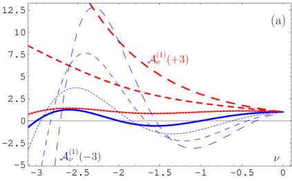
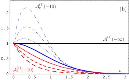
This estimate can be extended to any real value ν>1𝜈1\nu>1 of the index m𝑚m. To make the content of Eq. (30) more transparent, we display in Fig. 1(a) the graphs of the analytic coupling for indices from 33-3 to 0 and values of L𝐿L in the range 33-3 to 3.

Refer to caption    Refer to caption


Figure 1: (a): Comparison of different curves for 𝒜ν(1)(L)superscriptsubscript𝒜𝜈(1)𝐿{\cal A}_{\nu}^{\text{(1)}}(L) as functions of the index ν0𝜈0\nu\leq 0, corresponding to various values of L𝐿L, ranging from L=3𝐿3L=-3 to L=+3𝐿3L=+3. The blue broken lines correspond to L<0𝐿0L<0, whereas the red thick broken lines correspond to L>0𝐿0L>0. The two dotted lines denote the results for L=±1𝐿plus-or-minus1L=\pm 1, with the line associated with the value L=1𝐿1L=1 being closer to the zero line. (b): The same comparison for ν0𝜈0\nu\geq 0 using the same line designations, but for values of L𝐿L, ranging from L=10𝐿10L=-10 to L=+10𝐿10L=+10 (dashed lines). The dotted lines here correspond to L=±2𝐿plus-or-minus2L=\pm 2, whereas the short-dashed lines represent the result for L=±5𝐿plus-or-minus5L=\pm 5. The blue solid lines in both panels show 𝒜ν(1)(0)superscriptsubscript𝒜𝜈(1)0{\cal A}_{\nu}^{\text{(1)}}(0).

Appealing to Eqs. (34) and (35) for negative values of the index ν𝜈\nu, one makes sure that, for L=1𝐿1L=1 (red thick dotted line above the zero line), this function is equal to unity for all integer values of the index ν=m𝜈𝑚\nu=-m. On the other hand, for L<1𝐿1L<-1, the value of 𝒜m(L)subscript𝒜𝑚𝐿{\cal A}_{-m}(L) depends on whether or not m𝑚m is even or odd. For even values, it is positive, whereas for odd values it is negative, therefore giving rise to oscillations shown in Fig. 1(a). Note also that for values of L1𝐿1L\geq 1, the oscillatory behavior of the graphs for 𝒜ν(L)subscript𝒜𝜈𝐿{\cal A}_{\nu}(L) starts to be much less pronounced (red thick broken lines) because Lmsuperscript𝐿𝑚L^{m} is positive for all positive values of m𝑚m. The opposite behavior is exhibited for L<0𝐿0L<0, as one sees from the blue broken lines.

From Fig. 1(b), we observe that, in the region where 𝒜ν(L)subscript𝒜𝜈𝐿{\cal A}_{\nu}(L) is smaller than unity (as explicitly indicated in the figure), this function is monotonic in ν𝜈\nu for ν2𝜈2\nu\leq 2. On the other hand, in the region where 𝒜ν(L)>1subscript𝒜𝜈𝐿1{\cal A}_{\nu}(L)>1—possible only for ν<1𝜈1\nu<1 and L<0𝐿0L<0—this function starts to be non-monotonic in ν𝜈\nu, so that there are two different points ν1subscript𝜈1\nu_{1} and ν2subscript𝜈2\nu_{2}, both corresponding to the same value of 𝒜ν(L)subscript𝒜𝜈𝐿{\cal A}_{\nu}(L). Focusing on the values of 𝒜ν(L)subscript𝒜𝜈𝐿{\cal A}_{\nu}(L) for L>0𝐿0L>0, we see that all curves are monotonic in L𝐿L and are bounded by an envelope represented by 𝒜ν(0)subscript𝒜𝜈0{\cal A}_{\nu}(0) (the blue thick solid line in Fig. 1(b)). If we consider only the interval of ν(0,1)𝜈01\nu\in(0,1), then the monotonicity property extends also to the negative values of L𝐿L.

Contrary to that case, the coupling 𝒜m(L)subscript𝒜𝑚𝐿{\cal A}_{m}(L) oscillates in L𝐿L Shi98 for higher values of m>2𝑚2m>2. These oscillations are not visible in Fig. 1(b) because of the smallness of the corresponding amplitudes. They appear due to rather general reasons:
   (i) the asymptotic conditions given by Eq. (33): 𝒜m()=𝒜m()=0subscript𝒜𝑚subscript𝒜𝑚0{\cal A}_{m}(-\infty)={\cal A}_{m}(\infty)=0 for m2𝑚2m\geq 2;
   (ii) the differential relation between 𝒜msubscript𝒜𝑚{\cal A}_{m} and 𝒜1subscript𝒜1{\cal A}_{1}, expressed in Eq. (18).
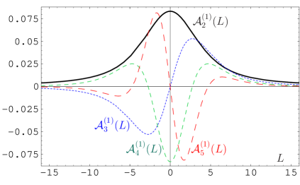
Therefore, 𝒜m+2subscript𝒜𝑚2{\cal A}_{m+2} has m𝑚m zeros in the vicinity of the former “Landau pole” (L=0𝐿0L=0) Shi98 —see Fig. 2. This property is rather unexpected from the point of view of standard power-series perturbation theory and will be discussed below in connection with Eq. (39).
Refer to caption


Figure 2: Comparison of different curves for 𝒜m(1)(L)superscriptsubscript𝒜𝑚(1)𝐿{\cal A}_{m}^{\text{(1)}}(L) as functions of L𝐿L, corresponding to various values of the index m𝑚m, ranging from m=2𝑚2m=2 to m=5𝑚5m=5. To show all the details in a single plot, higher couplings are multiplied by numerical factors in order to normalize them to the scale of 𝒜2(1)(L)superscriptsubscript𝒜2(1)𝐿{\cal A}_{2}^{\text{(1)}}(L). The solid line shows 𝒜2(1)(L)superscriptsubscript𝒜2(1)𝐿{\cal A}_{2}^{\text{(1)}}(L), the blue dotted line corresponds to 8𝒜3(1)(L)8superscriptsubscript𝒜3(1)𝐿8\cdot{\cal A}_{3}^{\text{(1)}}(L), the green short-dashed line to 60𝒜4(1)(L)60superscriptsubscript𝒜4(1)𝐿60\cdot{\cal A}_{4}^{\text{(1)}}(L), and the red long-dashed line to 480𝒜5(1)(L)480superscriptsubscript𝒜5(1)𝐿480\cdot{\cal A}_{5}^{\text{(1)}}(L).

This oscillation property of the coupling extends to 𝒜ν(L)subscript𝒜𝜈𝐿{\cal A}_{\nu}(L) for all real values of the index ν2𝜈2\nu\geq 2.

To reveal the relevance of this representation for physical applications, let us now consider 𝒜𝒜{\cal A} for some particular values of the index ν𝜈\nu. For the case of a negative index, the 𝒜νsubscript𝒜𝜈{\cal A}_{-\nu} play the role of the “inverse powers” of 𝒜1subscript𝒜1{\cal A}_{1} that may be considered as the images of asνsuperscriptsubscript𝑎𝑠𝜈a_{s}^{-\nu}. Then, expression (30) can be rewritten in the form

𝒜ν(L)subscript𝒜𝜈𝐿\displaystyle{\cal A}_{-\nu}(L) =\displaystyle= LνLiν+1(eL)Γ(ν),superscript𝐿𝜈Liν+1superscript𝑒𝐿Γ𝜈\displaystyle L^{\nu}-\frac{\textbf{Li${}_{\nu+1}$}(e^{-L})}{\Gamma(-\nu)}\,, (34)
𝒜m(L)=limε0𝒜m+ε(L)subscript𝒜𝑚𝐿subscript𝜀0subscript𝒜𝑚𝜀𝐿\displaystyle{\cal A}_{-m}(L)=\lim_{\varepsilon\to 0}{\cal A}_{-m+\varepsilon}(L) =\displaystyle= Lm,atm=0,1,2,,formulae-sequencesuperscript𝐿𝑚at𝑚012\displaystyle L^{m}\,,~{}~{}~{}\text{at}~{}~{}m=0,1,2,\ldots\,, (35)

where we have taken into account that for ν0𝜈0\nu\geq 0

F(z,ν)=Liν(z),𝐹𝑧𝜈Liν𝑧\displaystyle F(z,\nu)=\textbf{Li${}_{\nu}$}(z)\,, (36)

with Liν being the well-known polylogarithm function. It is worth remarking here that the “inverse powers” 𝒜m(L)=Lmsubscript𝒜𝑚𝐿superscript𝐿𝑚{\cal A}_{-m}(L)=L^{m} coincide with the inverse powers of the original running coupling am(L)=Lmsuperscript𝑎𝑚𝐿superscript𝐿𝑚a^{-m}(L)=L^{m}.

To make explicit the properties of Eq. (30), we convert this equation into a series representation, using Eq. (62), to obtain

F(z,1ν)𝐹𝑧1𝜈\displaystyle F(z,1-\nu) =\displaystyle= Γ(ν)[ln(1z)]ν+r=0ζ(1νr)lnr(z)r!Γ𝜈superscriptdelimited-[]1𝑧𝜈superscriptsubscript𝑟0𝜁1𝜈𝑟superscript𝑟𝑧𝑟\displaystyle\Gamma(\nu)\left[\ln\left(\frac{1}{z}\right)\right]^{-\nu}+\sum_{r=0}^{\infty}\zeta(1-\nu-r)\frac{\ln^{r}(z)}{r!} (37)

for |ln(z)|<2π𝑧2𝜋|\ln(z)|<2\pi, where ζ(ν)𝜁𝜈\zeta(\nu) is the Riemann ζ𝜁\zeta-function. Now we are in the position to express 𝒜νsubscript𝒜𝜈{\cal A}_{\nu} in the form of a series, i.e.,

𝒜ν(L)=1Γ(ν)r=0ζ(1νr)(L)rr!for|L|<2πformulae-sequencesubscript𝒜𝜈𝐿1Γ𝜈superscriptsubscript𝑟0𝜁1𝜈𝑟superscript𝐿𝑟𝑟for𝐿2𝜋\displaystyle{\cal A}_{\nu}(L)=-\frac{1}{\Gamma(\nu)}\sum_{r=0}^{\infty}\zeta(1-\nu-r)\frac{(-L)^{r}}{r!}~{}~{}~{}~{}~{}\text{for}~{}|L|<2\pi (38)

because the “standard logarithms”, contained in both parts of expression (30), mutually cancel, as one verifies by substituting Eq. (37) into Eq. (30). Then, we can state the following important corollaries:

  1. 1.

    𝒜ν(0)=ζ(1ν)Γ(ν)subscript𝒜𝜈0𝜁1𝜈Γ𝜈\displaystyle{\cal A}_{\nu}(0)=-\frac{\zeta(1-\nu)}{\Gamma(\nu)} is an entire function of ν𝜈\nu.
    Of particular importance are the following values:

    𝒜1(0)=12,𝒜2(0)=112,𝒜3(0)=0,𝒜4(0)=1720,𝒜5(0)=0formulae-sequencesubscript𝒜1012formulae-sequencesubscript𝒜20112formulae-sequencesubscript𝒜300formulae-sequencesubscript𝒜401720subscript𝒜500\displaystyle\displaystyle{\cal A}_{1}(0)=\frac{1}{2},~{}~{}~{}\displaystyle{\cal A}_{2}(0)=\frac{1}{12},~{}~{}~{}\displaystyle{\cal A}_{3}(0)=0,~{}~{}~{}\displaystyle{\cal A}_{4}(0)=-\frac{1}{720},~{}~{}~{}\displaystyle{\cal A}_{5}(0)=0 (39)

    that coincide with the results provided in Shi98 . Note that 𝒜2n+1(0)=0subscript𝒜2𝑛100{\cal A}_{2n+1}(0)=0 for n1𝑛1n\geq 1 is due to the property ζ(2n)=0𝜁2𝑛0\zeta(-2n)=0, while the set of 𝒜2n(0)subscript𝒜2𝑛0{\cal A}_{2n}(0) is alternating in sign BE53 . These properties illustrate the details of the coupling oscillations in the vicinity of L=0𝐿0L=0 for index values m>2𝑚2m>2. A convenient series representation of 𝒜msubscript𝒜𝑚{\cal A}_{m} for an integer index m𝑚m is presented and discussed in Appendix A (item 3).

  2. 2.

    Taking into account the relation limϵ0ζ(1ϵr)Γ(ϵ)=δ0rsubscriptitalic-ϵ0𝜁1italic-ϵ𝑟Γitalic-ϵsubscript𝛿0𝑟\displaystyle-\lim_{\epsilon\to 0}\frac{\zeta(1-\epsilon-r)}{\Gamma(\epsilon)}=\delta_{0r}, (see, e.g., Eq. (66)), one can take the limit

    𝒜0(L)=limν0𝒜ν(L)=1,subscript𝒜0𝐿subscript𝜈0subscript𝒜𝜈𝐿1\displaystyle{\cal A}_{0}(L)=\lim_{\nu\to 0}{\cal A}_{\nu}(L)=1\,, (40)

    dispensing with the constraint |L|<2π𝐿2𝜋|L|<2\pi and proving assertion (8).

  3. 3.

    Equation (35) can be re-derived from representation (38) in a way similar to that described in the previous item.

The upshot of these considerations is that the linear space {𝒜n}subscript𝒜𝑛\{{\cal A}_{n}\} is now completed via the inclusion of the elements 𝒜νsubscript𝒜𝜈{\cal A}_{\nu} for any real values of the index ν𝜈\nu, so that one can take derivatives with respect to this continuous variable—dubbed ‘index derivative’.

III.3 Analytic images of products of coupling powers and logarithms

To this point, we have considered only powers of the running coupling, adopting the viewpoint of the Shirkov–Solovtsov APT. Now we are going to consider more complicated expressions, like (a(l))νLmsuperscriptsubscript𝑎𝑙𝜈superscript𝐿𝑚\left(a_{(l)}\right)^{\nu}L^{m}, where the power ν𝜈\nu is a real number and the power m𝑚m is an integer, following the broader “analytization” principle of KS KS01 ; Ste02 .

To compute this image, we have first to determine the image of aνln(a)superscript𝑎𝜈𝑎a^{\nu}\ln(a), which can be rewritten as the derivative of aνsuperscript𝑎𝜈a^{\nu} with respect to ν𝜈\nu; viz.,

aνln(a)=ddνaν.superscript𝑎𝜈𝑎𝑑𝑑𝜈superscript𝑎𝜈\displaystyle a^{\nu}\ln(a)=\frac{d}{d\nu}\,a^{\nu}\,. (41)

Due to the linearity of the differential operator, this derivative can be directly applied to any element of the completed space {𝒜n}subscript𝒜𝑛\{{\cal A}_{n}\} to generate the corresponding image, [aνln(a)]ansubscriptdelimited-[]superscript𝑎𝜈𝑎an\left[a^{\nu}\ln(a)\right]_{\text{an}}, and define

[ddνaν]an=defddν𝒜ν.superscript𝑑𝑒𝑓subscriptdelimited-[]𝑑𝑑𝜈superscript𝑎𝜈an𝑑𝑑𝜈subscript𝒜𝜈\displaystyle\left[\frac{d}{d\nu}\,a^{\nu}\right]_{\text{an}}\stackrel{{\scriptstyle def}}{{=}}\frac{d}{d\nu}\,{\cal A}_{\nu}\,. (42)

In the following, we shall employ for the sake of simplicity a special notation for the derivatives with respect to the index of the non-power expansion and define

𝒟k𝒜νdkdνk𝒜ν.superscript𝒟𝑘subscript𝒜𝜈superscript𝑑𝑘𝑑superscript𝜈𝑘subscript𝒜𝜈\displaystyle{\cal D}^{k}\,{\cal A}_{\nu}\equiv\frac{d^{k}}{d\nu^{k}}\,{\cal A}_{\nu}\,. (43)

From Eqs. (30) and (42), we obtain

[aνln(a)]an=lnLLνddν(F(eL,1ν)Γ(ν))subscriptdelimited-[]superscript𝑎𝜈𝑎an𝐿superscript𝐿𝜈𝑑𝑑𝜈𝐹superscript𝑒𝐿1𝜈Γ𝜈\displaystyle\left[a^{\nu}\ln(a)\right]_{\text{an}}=-\frac{\ln L}{L^{\nu}}-\frac{d}{d\nu}\,\left(\frac{F(e^{-L},1-\nu)}{\Gamma(\nu)}\right) (44)

and taking multiple derivatives on both sides of Eq. (42), we compute the image of aνLmsuperscript𝑎𝜈superscript𝐿𝑚a^{\nu}L^{m}, like in Eq. (44). This procedure applies to any desired degree m𝑚m of such terms.

The extension to higher loops makes use of the APT expansion of higher-loop quantities in terms of one-loop ones. Before doing that, we consider first the image of a(2)subscript𝑎2a_{(2)} on the basis of the perturbation expansion, given in Eq. (73) in conjunction with Eq. (43), to obtain the element 𝒜1subscript𝒜1{\cal A}_{1} at the two-loop level:

𝒜1(2)(L)=𝒜1(1)+c1𝒟𝒜ν=2(1)+c12(𝒟2+𝒟11)𝒜ν=3(1)+𝒪(𝒟3𝒜ν=4(1)).superscriptsubscript𝒜12𝐿superscriptsubscript𝒜11subscript𝑐1𝒟superscriptsubscript𝒜𝜈21superscriptsubscript𝑐12superscript𝒟2superscript𝒟11superscriptsubscript𝒜𝜈31𝒪superscript𝒟3superscriptsubscript𝒜𝜈41\displaystyle{\cal A}_{1}^{(2)}(L)={\cal A}_{1}^{(1)}+c_{1}\,{\cal D}\,{\cal A}_{\nu=2}^{(1)}+c_{1}^{2}\,\left({\cal D}^{2}+{\cal D}^{1}-1\right)\,{\cal A}_{\nu=3}^{(1)}+{\cal O}\left({\cal D}^{3}\,{\cal A}_{\nu=4}^{(1)}\right)\,. (45)

This formula can be readily generalized to any index ν𝜈\nu:

𝒜ν(2)(L)superscriptsubscript𝒜𝜈2𝐿\displaystyle{\cal A}_{\nu}^{(2)}(L) =\displaystyle= 𝒜ν(1)+c1ν𝒟𝒜ν+1(1)+c12ν[(1+ν)2𝒟2+𝒟11]𝒜ν+2(1)superscriptsubscript𝒜𝜈1subscript𝑐1𝜈𝒟superscriptsubscript𝒜𝜈11superscriptsubscript𝑐12𝜈delimited-[]1𝜈2superscript𝒟2superscript𝒟11superscriptsubscript𝒜𝜈21\displaystyle{\cal A}_{\nu}^{(1)}+c_{1}\,\nu\,{\cal D}\,{\cal A}_{\nu+1}^{(1)}+c_{1}^{2}\,\nu\left[\,\frac{\left(1+\nu\right)}{2}{\cal D}^{2}\,+\,{\cal D}^{1}\,-1\right]{\cal A}_{\nu+2}^{(1)} (46)
+𝒪(𝒟3𝒜ν+3(1)),𝒪superscript𝒟3superscriptsubscript𝒜𝜈31\displaystyle+\,{\cal O}\left({\cal D}^{3}\,{\cal A}_{\nu+3}^{(1)}\right)\,,

where c1=b1/b02subscript𝑐1subscript𝑏1superscriptsubscript𝑏02c_{1}=b_{1}/b_{0}^{2} is an auxiliary expansion parameter. The quality of the two-loop approximation for the lowest index (cf. Eq. (45)) and higher indices (cf. Eq. (46)) will be analyzed numerically in the next section. Here it suffices to mention that the achieved accuracy is of the order of about 1%percent11\% down to L=0𝐿0L=0.

To construct the image of (a(2))νLsuperscriptsubscript𝑎2𝜈𝐿\left(a_{(2)}\right)^{\nu}L, cf. Eq. (12), we first perform the “analytization” of Eq. (75) and then use Eq. (42) to arrive at the final expression

[(a(2)(L))νL]anν,1(2)(L)subscriptdelimited-[]superscriptsubscript𝑎2𝐿𝜈𝐿ansuperscriptsubscript𝜈12𝐿\displaystyle\left[\left(a_{(2)}(L)\right)^{\nu}L\right]_{\text{an}}\equiv{\cal L}_{\nu,1}^{(2)}(L) =\displaystyle= 𝒜ν1(2)+c1𝒟𝒜ν(2)+𝒪(𝒜ν+1(2)),superscriptsubscript𝒜𝜈12subscript𝑐1𝒟superscriptsubscript𝒜𝜈2𝒪superscriptsubscript𝒜𝜈12\displaystyle{\cal A}_{\nu-1}^{(2)}+c_{1}\,{\cal D}\,{\cal A}_{\nu}^{(2)}+{\cal O}\left({\cal A}_{\nu+1}^{(2)}\right)\,, (47)

which can be recast, by means of the one-loop analytic coupling and with the aid of Eq. (44), in the form

ν,1(2)(L)=𝒜ν1(1)c1ν[ln(L)ψ(ν)Lν+ψ(ν)𝒜ν(1)+𝒟F(eL,1ν)Γ(ν)]+𝒪(𝒟2𝒜ν+1(1)).superscriptsubscript𝜈12𝐿superscriptsubscript𝒜𝜈11subscript𝑐1𝜈delimited-[]𝐿𝜓𝜈superscript𝐿𝜈𝜓𝜈superscriptsubscript𝒜𝜈1𝒟𝐹superscript𝑒𝐿1𝜈Γ𝜈𝒪superscript𝒟2superscriptsubscript𝒜𝜈11\displaystyle{\cal L}_{\nu,1}^{(2)}(L)={\cal A}_{\nu-1}^{(1)}-c_{1}\nu\left[\frac{\ln(L)-\psi(\nu)}{L^{\nu}}+\psi(\nu){\cal A}_{\nu}^{(1)}+\frac{{\cal D}F(e^{-L},1-\nu)}{\Gamma(\nu)}\right]+{\cal O}\left({\cal D}^{2}\,{\cal A}_{\nu+1}^{(1)}\right)\!.~{}~{}~{}~{} (48)

The “analytization” of (a(2)(L))νL2superscriptsubscript𝑎2𝐿𝜈superscript𝐿2\left(a_{(2)}(L)\right)^{\nu}\cdot L^{2}, expressed in terms of Eq. (77), can be performed in an analogous way with the result

ν,2(2)(L)superscriptsubscript𝜈22𝐿\displaystyle{\cal L}_{\nu,2}^{(2)}(L) =\displaystyle= 𝒜ν2(2)+2c1𝒟𝒜ν1(2)+c12𝒟2𝒜ν(2)2c12𝒜ν(2)+𝒪(𝒟𝒜ν+1(2)).superscriptsubscript𝒜𝜈222subscript𝑐1𝒟superscriptsubscript𝒜𝜈12superscriptsubscript𝑐12superscript𝒟2superscriptsubscript𝒜𝜈22superscriptsubscript𝑐12superscriptsubscript𝒜𝜈2𝒪𝒟superscriptsubscript𝒜𝜈12\displaystyle{\cal A}_{\nu-2}^{(2)}+2c_{1}\,{\cal D}\,{\cal A}_{\nu-1}^{(2)}+c_{1}^{2}\,{\cal D}^{2}\,{\cal A}_{\nu}^{(2)}-2c_{1}^{2}\,{\cal A}_{\nu}^{(2)}+{\cal O}\left({\cal D}\,{\cal A}_{\nu+1}^{(2)}\right)\,. (49)

The one-loop approximation of this two-loop expression is given by

ν,2(2)(L)=𝒜ν2(1)+c1ν𝒟𝒜ν1(1)+c12ν2ν+42𝒟2𝒜ν(1)+𝒪(𝒟𝒜ν+1(1)).superscriptsubscript𝜈22𝐿superscriptsubscript𝒜𝜈21subscript𝑐1𝜈𝒟superscriptsubscript𝒜𝜈11superscriptsubscript𝑐12superscript𝜈2𝜈42superscript𝒟2superscriptsubscript𝒜𝜈1𝒪𝒟superscriptsubscript𝒜𝜈11\displaystyle{\cal L}_{\nu,2}^{(2)}(L)={\cal A}_{\nu-2}^{(1)}+c_{1}\,\nu\,{\cal D}\,{\cal A}_{\nu-1}^{(1)}+c_{1}^{2}\,\frac{\nu^{2}-\nu+4}{2}\,{\cal D}^{2}\,{\cal A}_{\nu}^{(1)}+{\cal O}\left({\cal D}\,{\cal A}_{\nu+1}^{(1)}\right)\,. (50)

A compilation of the required formulae to achieve the “analytization” of powers of the coupling in conjunction with logarithms at the two-loop order, is provided in Appendix B.

Up to now we have studied expressions appearing in fixed-order perturbation theory. But similar considerations apply also to resummed perturbation theory. Indeed, first attempts to apply the “analytization” procedure of Shirkov–Solovtsov were already presented in SSK99 ; SSK00 ; Ste02 . The crucial point here is how to deal with the requirement of analyticity when performing a Sudakov resummation. Because of the non-power series character of APT, resummation of (soft-gluon) logarithms does not lead to exponentiation. The latter can be retained only in the case of the so-called naive “analytization” BPSS04 , proposed in SSK99 ; SSK00 . The exact expression for the Sudakov factor is too complicated and too specific to be discussed in the present analysis. We, therefore, consider in Appendix C a simplified version of a ‘toy Sudakov’ factor that, nevertheless, bears the key characteristics pertaining to resummation under the assertion of analyticity.

Table 1: Comparison of the standard PT, APT, and FAPT with L=ln(Q2/Λ2)𝐿superscript𝑄2superscriptΛ2\displaystyle L=\ln\left(Q^{2}/\Lambda^{2}\right).
 Theory Space Series expansion Inverse powers Multiplication Index derivative
 PT {a(l)ν}νsubscriptsuperscriptsubscript𝑎𝑙𝜈𝜈\Big{\{}a_{(l)}^{\nu}\Big{\}}_{\nu\in\mathbb{R}}\vphantom{{}^{\Big{|}}_{\Big{|}}} F(L)=mfma(l)m(L)𝐹𝐿subscript𝑚subscript𝑓𝑚superscriptsubscript𝑎𝑙𝑚𝐿F(L)=\sum\limits_{m}f_{m}\,a_{(l)}^{m}(L) (a(l)(L))msuperscriptsubscript𝑎𝑙𝐿𝑚\left(a_{(l)}(L)\right)^{-m} a(l)μa(l)ν=a(l)μ+νsuperscriptsubscript𝑎𝑙𝜇superscriptsubscript𝑎𝑙𝜈superscriptsubscript𝑎𝑙𝜇𝜈a_{(l)}^{\mu}a_{(l)}^{\nu}=a_{(l)}^{\mu+\nu} a(l)mlnka(l)superscriptsubscript𝑎𝑙𝑚superscript𝑘subscript𝑎𝑙a_{(l)}^{m}\ln^{k}a_{(l)}
APT {𝒜m(l)}msubscriptsubscriptsuperscript𝒜𝑙𝑚𝑚\Big{\{}{\cal A}^{(l)}_{m}\Big{\}}_{m\in\mathbb{N}}\vphantom{{}^{\Big{|}}_{\Big{|}}} (L)=mfm𝒜m(l)(L)𝐿subscript𝑚subscript𝑓𝑚subscriptsuperscript𝒜𝑙𝑚𝐿{\cal F}(L)=\sum\limits_{m}f_{m}\,{\cal A}^{(l)}_{m}(L) No No No
FAPT {𝒜ν(l)}νsubscriptsubscriptsuperscript𝒜𝑙𝜈𝜈\Big{\{}{\cal A}^{(l)}_{\nu}\Big{\}}_{\nu\in\mathbb{R}}\vphantom{{}^{\Big{|}}_{\Big{|}}} (L)=mfm𝒜m(l)(L)𝐿subscript𝑚subscript𝑓𝑚subscriptsuperscript𝒜𝑙𝑚𝐿{\cal F}(L)=\sum\limits_{m}f_{m}\,{\cal A}^{(l)}_{m}(L) 𝒜m(1)(L)=Lmsuperscriptsubscript𝒜𝑚1𝐿superscript𝐿𝑚{\cal A}_{-m}^{(1)}(L)=L^{m} No 𝒟k𝒜m(l)superscript𝒟𝑘subscriptsuperscript𝒜𝑙𝑚{\cal D}^{k}{\cal A}^{(l)}_{m}

For clarity, we compare the basic ingredients of FAPT in Table 1 with their counterparts in conventional perturbation theory and APT. More detailed expressions are shown in Table 2 in the next section.

IV Validation of the new scheme

IV.1 Analytic verification of the one-loop spectral density

An alternative way to derive Eq. (17) for the spectral density ρνsubscript𝜌𝜈\rho_{\nu}, is to compare two different representations for 𝒜νsubscript𝒜𝜈{\cal A}_{\nu}: one given by the dispersion relation, Eq. (3), and the other provided by the Laplace representation, Eq. (20). Then, we get

𝒜ν(L)=0ρν(σ)σ+Q2𝑑σ=0eLt𝒜~ν(t)𝑑t.subscript𝒜𝜈𝐿superscriptsubscript0subscript𝜌𝜈𝜎𝜎superscript𝑄2differential-d𝜎superscriptsubscript0superscript𝑒𝐿𝑡subscript~𝒜𝜈𝑡differential-d𝑡\displaystyle{\cal A}_{\nu}(L)=\int_{0}^{\infty}\!\frac{\rho_{\nu}(\sigma)}{\sigma+Q^{2}}\,d\sigma\,=\int_{0}^{\infty}e^{-Lt}~{}\tilde{{\cal A}}_{\nu}(t)~{}dt\,. (51)

Next, we make a double Borel transformation of both representations, the Laplace one and that of the dispersion integral, the aim being to extract ρν(σ)subscript𝜌𝜈𝜎\rho_{\nu}(\sigma). This is done by applying first M2B^(M2Q2)superscript𝑀2subscript^𝐵superscript𝑀2superscript𝑄2M^{2}\,\hat{B}_{(M^{2}\to Q^{2})} on both sides of Eq. (51) and then employing

M2B^(M2Q2)(1σ+Q2)=exp(σ/M2),M2B^(M2Q2)(Λ2Q2)t=M2Γ(t)(Λ2M2)t.formulae-sequencesuperscript𝑀2subscript^𝐵superscript𝑀2superscript𝑄21𝜎superscript𝑄2𝜎superscript𝑀2superscript𝑀2subscript^𝐵superscript𝑀2superscript𝑄2superscriptsuperscriptΛ2superscript𝑄2𝑡superscript𝑀2Γ𝑡superscriptsuperscriptΛ2superscript𝑀2𝑡\displaystyle M^{2}\,\hat{B}_{(M^{2}\to Q^{2})}\left(\frac{1}{\sigma+Q^{2}}\right)=\exp(-\sigma/M^{2})\,,~{}~{}M^{2}\,\hat{B}_{(M^{2}\to Q^{2})}\left(\frac{\Lambda^{2}}{Q^{2}}\right)^{t}=\frac{M^{2}}{\Gamma(t)}\left(\frac{\Lambda^{2}}{M^{2}}\right)^{t}\,. (52)

In the second step, we carry out one more Borel transformation, B^(𝟏/𝝈1/M2)subscript^𝐵1𝝈1superscript𝑀2\hat{B}_{(\bm{1/\sigma}\to 1/M^{2})}, to obtain

ρν(σ)=0(Λ2σ)tsin(πt)π𝒜~ν(t)𝑑t.subscript𝜌𝜈𝜎superscriptsubscript0superscriptsuperscriptΛ2𝜎𝑡𝜋𝑡𝜋subscript~𝒜𝜈𝑡differential-d𝑡\displaystyle\rho_{\nu}(\sigma)=\int_{0}^{\infty}\left(\frac{\Lambda^{2}}{\sigma}\right)^{t}\frac{\sin(\pi t)}{\pi}\,\tilde{{\cal A}}_{\nu}(t)~{}dt\,. (53)

The final step is to substitute in Eq. (53) the expression for A~ν(t)subscript~𝐴𝜈𝑡\tilde{A}_{\nu}(t), given by Eq. (24), to arrive at the final result

ρν(σ)subscript𝜌𝜈𝜎\displaystyle\rho_{\nu}(\sigma) =\displaystyle= 1(π2+L2(σ))ν/2sin[νarccos(L(σ)L2(σ)+π2)]1superscriptsuperscript𝜋2superscript𝐿2𝜎𝜈2𝜈𝐿𝜎superscript𝐿2𝜎superscript𝜋2\displaystyle\frac{1}{\left(\pi^{2}+L^{2}(\sigma)\right)^{\nu/2}}\sin\left[\nu\arccos\left(\frac{L(\sigma)}{\sqrt{L^{2}(\sigma)+\pi^{2}}}\right)\right] (54)
=\displaystyle= 1(π2+L2(σ))ν/2sin[νarctan(πL(σ))]forL(σ)>0,1superscriptsuperscript𝜋2superscript𝐿2𝜎𝜈2𝜈𝜋𝐿𝜎for𝐿𝜎0\displaystyle\frac{1}{\left(\pi^{2}+L^{2}(\sigma)\right)^{\nu/2}}\sin\left[\nu\arctan\left(\frac{\pi}{L(\sigma)}\right)\right]~{}\text{for}~{}L(\sigma)>0\,, (55)

where L(σ)=ln(σ/Λ2)𝐿𝜎𝜎superscriptΛ2L(\sigma)=\ln\left(\sigma/\Lambda^{2}\right). To gain a more complete understanding of the role of the Landau pole remover in 𝒜~νsubscript~𝒜𝜈\tilde{{\cal A}}_{\nu}, it is important to remark that it does not contribute to the spectral density, the reason being that this part is not altering the nature of the discontinuity. The latter is solely determined by the term 1/L1𝐿1/L. One appreciates that expressions (55) and (17) coincide, as they should, hence establishing the equivalence between the two alternative extensions of the “analytization” procedure to fractional indices. The two-loop approximate expression for the spectral density is given in Appendix B.

IV.2 Verification of the two-loop approximations

Now look specifically at the quality of the two-loop expansion in FAPT. In doing so, we define the following quantities with the help of an auxiliary parameter c1subscript𝑐1c_{1} and the index derivative 𝒟𝒟{\cal D}, (as in Eq. (45)):

  • NLO, i.e., retaining terms of order c1subscript𝑐1c_{1}

    Δ2FAPT(L)superscriptsubscriptΔ2FAPT𝐿\displaystyle\Delta_{2}^{\text{FAPT}}(L) =\displaystyle= 1𝒜1(1)(L)+c1𝒟𝒜ν=2(1)(L)𝒜1(2)(L)1superscriptsubscript𝒜11𝐿subscript𝑐1𝒟superscriptsubscript𝒜𝜈21𝐿superscriptsubscript𝒜12𝐿\displaystyle 1-\frac{{\cal A}_{1}^{(1)}(L)+c_{1}\,{\cal D}{\cal A}_{\nu=2}^{(1)}(L)}{{\cal A}_{1}^{(2)}(L)} (56)
  • NNLO, i.e., retaining terms up to order c12superscriptsubscript𝑐12c_{1}^{2}

    Δ3FAPT(L)superscriptsubscriptΔ3FAPT𝐿\displaystyle\Delta_{3}^{\text{FAPT}}(L) =\displaystyle= 1𝒜1(1)(L)+c1𝒟𝒜ν=2(1)(L)+c12(𝒟2+𝒟11)𝒜ν=3(1)(L)𝒜1(2)(L).1superscriptsubscript𝒜11𝐿subscript𝑐1𝒟superscriptsubscript𝒜𝜈21𝐿superscriptsubscript𝑐12superscript𝒟2superscript𝒟11superscriptsubscript𝒜𝜈31𝐿superscriptsubscript𝒜12𝐿\displaystyle 1-\frac{{\cal A}_{1}^{(1)}(L)+c_{1}\,{\cal D}\,{\cal A}_{\nu=2}^{(1)}(L)+c_{1}^{2}\,\left({\cal D}^{2}+{\cal D}^{1}-1\right)\,{\cal A}_{\nu=3}^{(1)}(L)}{{\cal A}_{1}^{(2)}(L)}\,. (57)

Refer to caption Refer to caption


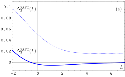
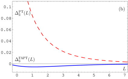
Figure 3: (a): The dotted line corresponds to Δ2FAPT(L)superscriptsubscriptΔ2FAPT𝐿\Delta_{2}^{\text{FAPT}}(L) and the solid line to Δ3FAPT(L)superscriptsubscriptΔ3FAPT𝐿\Delta_{3}^{\text{FAPT}}(L). (b): The dashed line corresponds to Δ3PT(L)superscriptsubscriptΔ3PT𝐿\Delta_{3}^{\text{PT}}(L) and the solid line to Δ3FAPT(L)superscriptsubscriptΔ3FAPT𝐿\Delta_{3}^{\text{FAPT}}(L).

For the corresponding quantities within the standard QCD perturbation theory, we use Eq. (73) to obtain

  • NLO, i.e., retaining terms of order c1subscript𝑐1c_{1}

    Δ2PT(L)=1a(1)(L)+c1a(1)2(L)lna(1)(L)a(2)(L)superscriptsubscriptΔ2PT𝐿1subscript𝑎1𝐿subscript𝑐1superscriptsubscript𝑎12𝐿subscript𝑎1𝐿subscript𝑎2𝐿\displaystyle\Delta_{2}^{\text{PT}}(L)=1-\frac{a_{(1)}(L)+c_{1}\,a_{(1)}^{2}(L)\,\ln a_{(1)}(L)}{a_{(2)}(L)} (58)
  • NNLO, i.e., retaining terms up to order c12superscriptsubscript𝑐12c_{1}^{2}

    Δ3PT(L)=1a(1)(L)+c1a(1)2(L)lna(1)(L)+c12a(1)3(L)(ln2a(1)(L)+lna(1)(L)1)a(2)(L).superscriptsubscriptΔ3PT𝐿1subscript𝑎1𝐿subscript𝑐1superscriptsubscript𝑎12𝐿subscript𝑎1𝐿superscriptsubscript𝑐12superscriptsubscript𝑎13𝐿superscript2subscript𝑎1𝐿subscript𝑎1𝐿1subscript𝑎2𝐿\displaystyle\!\!\!\!\!\!\!\Delta_{3}^{\text{PT}}(L)=1-\frac{a_{(1)}(L)+c_{1}\,a_{(1)}^{2}(L)\,\ln a_{(1)}(L)+c_{1}^{2}\,a_{(1)}^{3}(L)\,\left(\ln^{2}a_{(1)}(L)+\ln a_{(1)}(L)-1\right)}{a_{(2)}(L)}\,.
    (59)

Refer to caption   Refer to caption

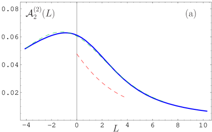
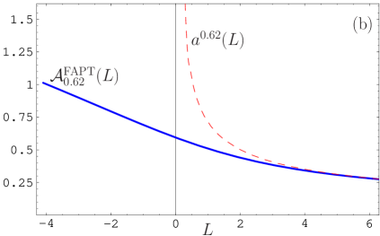
Figure 4: (a) Comparison of different results for 𝒜2(2)(L)superscriptsubscript𝒜22𝐿{\cal A}_{2}^{(2)}(L). The solid line corresponds to 𝒜2(2);FAPT(L)superscriptsubscript𝒜22FAPT𝐿{\cal A}_{2}^{(2);\text{FAPT}}(L), computed analytically via Eq. (46); 𝒜2(2);num(L)superscriptsubscript𝒜22num𝐿{\cal A}_{2}^{(2);\text{num}}(L) (dashed line) is derived by means of a numerical integration. The dotted line represents the available results of the numerical procedure of Magradze in Mag03u . (b) Comparison of FAPT and standard QCD PT with respect to the fractional index (power) of the coupling. The solid line represents 𝒜0.62(2);FAPT(L)superscriptsubscript𝒜0.622FAPT𝐿{\cal A}_{0.62}^{(2);\text{FAPT}}(L), computed analytically via Eq. (46), while the dashed line stands for a(2)0.62(L)subscriptsuperscript𝑎0.622𝐿a^{0.62}_{(2)}(L).

First, let us compare the transition from the NLO (cf. Eq. (56)) to the NNLO (cf. Eq. (57)) in FAPT (see Fig. 3(a)). One appreciates that by taking into account the NNLO terms, a significant improvement of the convergence quality of the FAPT series is achieved. Indeed, even at Q2=Λ2superscript𝑄2superscriptΛ2Q^{2}=\Lambda^{2}, which corresponds to L=0𝐿0L=0, the error of truncating the FAPT series at the NLO is about 5%, while by taking into account the NNLO correction this error becomes even smaller than 0.5%. In Fig. 3(b) we show the relative quality of these approximations concerning the loop expansion between the standard perturbation theory and FAPT, as quantified by Eqs. (57) and (59). One appreciates the strong suppression of Δ3FAPT(L)superscriptsubscriptΔ3FAPT𝐿\Delta_{3}^{\text{FAPT}}(L) relative to its conventional analogue in the small L𝐿L region, say, below approximately L=2𝐿2L=2.

The same comparison can be realized for 𝒜2(2)superscriptsubscript𝒜22{\cal A}_{2}^{(2)}, using Eq. (46). Indeed, we demonstrate in Fig. 4(a) the quality of this FAPT expansion in comparison with the results of the numerical integration of the NLO spectral density ρ2subscript𝜌2\rho_{2} (for more details, we refer to Appendix B and SS99 ) in the dispersion-integral representation, provided by Eq. (3). In this graphics, we also display the results obtained numerically by Magradze in Mag03u . The message from Fig. 4(a) is quite clear. Our analytic (solid line) and our numerical calculation (dashed line) are in mutual support, while the results of Mag03u differ considerably with respect to both the magnitude and the trend of the negative values of L𝐿L.

Refer to caption


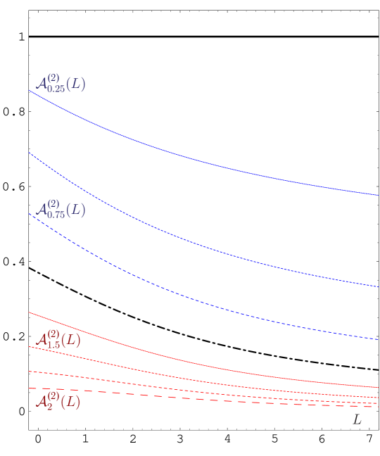
Figure 5: Analytic images 𝒜ν(2)(L)superscriptsubscript𝒜𝜈(2)𝐿{\cal A}_{\nu}^{\text{(2)}}(L) at the two-loop level for some characteristic index values,555We wish to thank D. V. Shirkov for suggesting to us this form of presentation. calculated with NNLO FAPT. The solid line corresponds to ν=0𝜈0\nu=0, the dash-dotted one to ν=1𝜈1\nu=1, and the lowest line to ν=2𝜈2\nu=2. All other lines correspond to ν=k/4𝜈𝑘4\nu=k/4 with k=1,,7𝑘17k=1,...,7.

The good convergence of the proposed series for 𝒜1,2(2)superscriptsubscript𝒜122{\cal A}_{1,2}^{(2)} (Eq. (46)), that had been demonstrated above, can be traced to the basis of APT. Indeed, this non-power expansion of the quantities 𝒜1,2(2)superscriptsubscript𝒜122{\cal A}_{1,2}^{(2)} in terms of 𝒜m(1)superscriptsubscript𝒜𝑚1{\cal A}_{m}^{(1)} has a finite radius of convergence, the reasons being discussed in Ref. Mik04 .

To give the reader an impression of the dependence on L𝐿L of 𝒜ν(2)(L)subscriptsuperscript𝒜2𝜈𝐿{\cal A}^{(2)}_{\nu}(L), we show in Fig. 4(b) a comparison of this quantity with its counterpart in standard QCD, namely, [a(2)(L)]νsuperscriptdelimited-[]subscript𝑎2𝐿𝜈\left[a_{(2)}(L)\right]^{\nu}. For the purpose of illustration, we select the value ν=γ2/(2b0)0.62𝜈subscript𝛾22subscript𝑏00.62\nu=\gamma_{2}/(2b_{0})\approx 0.62, which corresponds to the 1-loop evolution exponent of the non-singlet quark operator of index 2, entering a number of applications in DIS and also various exclusive reactions BMS02 ; BMS03 ; BMS01 .

Table 2: Calculational rules for FAPT with L=ln(Q2/Λ2)𝐿superscript𝑄2superscriptΛ2\displaystyle L=\ln\left(Q^{2}/\Lambda^{2}\right), m𝑚m\in\mathbb{N}, and ν𝜈\nu\in\mathbb{R}.
Standard QCD PT QCD FAPT
a(1)1(L)=1Lsubscriptsuperscript𝑎11𝐿1𝐿\displaystyle a^{1}_{(1)}(L)=\frac{1}{L}\vphantom{{}^{\Big{|}}_{\Big{|}}} 𝒜1(1)(L)=1L1eL1superscriptsubscript𝒜11𝐿1𝐿1superscript𝑒𝐿1\displaystyle{\cal A}_{1}^{(1)}(L)=\frac{1}{L}-\frac{1}{e^{L}-1}
a(1)ν(L)=1Lνsubscriptsuperscript𝑎𝜈1𝐿1superscript𝐿𝜈\displaystyle a^{\nu}_{(1)}(L)=\frac{1}{L^{\nu}}\vphantom{{}^{\Big{|}}_{\Big{|}}} 𝒜ν(1)(L)=1LνF(eL,1ν)Γ(ν)superscriptsubscript𝒜𝜈1𝐿1superscript𝐿𝜈𝐹superscript𝑒𝐿1𝜈Γ𝜈\displaystyle{\cal A}_{\nu}^{(1)}(L)=\frac{1}{L^{\nu}}-\frac{F(e^{-L},1-\nu)}{\Gamma(\nu)}
a(l)ν(L)lnm[a(l)(L)]subscriptsuperscript𝑎𝜈𝑙𝐿superscript𝑚subscript𝑎𝑙𝐿\displaystyle a^{\nu}_{(l)}(L)\,\ln^{m}\left[a_{(l)}(L)\right]\vphantom{{}^{\Big{|}}_{\Big{|}}} 𝒟m𝒜ν(l)(L)dmdνm[𝒜ν(l)(L)]superscript𝒟𝑚superscriptsubscript𝒜𝜈𝑙𝐿superscript𝑑𝑚𝑑superscript𝜈𝑚delimited-[]superscriptsubscript𝒜𝜈𝑙𝐿\displaystyle{\cal D}^{m}\,{\cal A}_{\nu}^{(l)}(L)\equiv\frac{d^{m}}{d\nu^{m}}\,\left[{\cal A}_{\nu}^{(l)}(L)\right]
a(2)ν(L)subscriptsuperscript𝑎𝜈2𝐿\displaystyle a^{\nu}_{(2)}(L)\vphantom{{}^{\Big{|}}_{\big{|}}} 𝒜ν(2)(L)=𝒜ν(1)(L)+c1ν𝒟𝒜ν+1(1)(L)+c12ν[(ν+1)2𝒟2+𝒟1]𝒜ν+2(1)(L)superscriptsubscript𝒜𝜈2𝐿superscriptsubscript𝒜𝜈1𝐿subscript𝑐1𝜈𝒟superscriptsubscript𝒜𝜈11𝐿superscriptsubscript𝑐12𝜈delimited-[]𝜈12superscript𝒟2𝒟1superscriptsubscript𝒜𝜈21𝐿\displaystyle{\cal A}_{\nu}^{(2)}(L)={\cal A}_{\nu}^{(1)}(L)+c_{1}\nu\,{\cal D}\,{\cal A}_{\nu+1}^{(1)}(L)+c_{1}^{2}\,\nu\left[\frac{(\nu+1)}{2}{\cal D}^{2}+{\cal D}-1\right]\!{\cal A}_{\nu+2}^{(1)}(L)
                 +𝒪(𝒟3𝒜ν+3(1))𝒪superscript𝒟3superscriptsubscript𝒜𝜈31+~{}{\cal O}\left({\cal D}^{3}\,{\cal A}_{\nu+3}^{(1)}\right)\vphantom{{}_{\Big{|}}}666Note that in evaluating this expression in the next line we use Eqs. (74) and (30).
a(2)ν(L)Lsubscriptsuperscript𝑎𝜈2𝐿𝐿\displaystyle a^{\nu}_{(2)}(L)\,L\vphantom{{}^{\Big{|}}_{\big{|}}} ν,1(2)(L)=𝒜ν1(2)(L)+c1𝒟𝒜ν(2)(L)+𝒪(𝒟2𝒜ν+1(2))superscriptsubscript𝜈12𝐿superscriptsubscript𝒜𝜈12𝐿subscript𝑐1𝒟superscriptsubscript𝒜𝜈2𝐿𝒪superscript𝒟2superscriptsubscript𝒜𝜈12\displaystyle{\cal L}_{\nu,1}^{(2)}(L)={\cal A}_{\nu-1}^{(2)}(L)+c_{1}\,{\cal D}\,{\cal A}_{\nu}^{(2)}(L)+{\cal O}\left({\cal D}^{2}\,{\cal A}_{\nu+1}^{(2)}\right)777Note that in evaluating this expression in the next line we use Eqs. (76), (77), and (30).
𝒜ν1(1)(L)c1ν[ln(L)ψ(ν)Lν+ψ(ν)𝒜ν(1)(L)+𝒟F(eL,1ν)Γ(ν)]absentsuperscriptsubscript𝒜𝜈11𝐿subscript𝑐1𝜈delimited-[]𝐿𝜓𝜈superscript𝐿𝜈𝜓𝜈superscriptsubscript𝒜𝜈1𝐿𝒟𝐹superscript𝑒𝐿1𝜈Γ𝜈\displaystyle\approx{\cal A}_{\nu-1}^{(1)}(L)-c_{1}\nu\left[\frac{\ln(L)-\psi(\nu)}{L^{\nu}}+\psi(\nu){\cal A}_{\nu}^{(1)}(L)+\frac{{\cal D}F(e^{-L},1-\nu)}{\Gamma(\nu)}\right]\vphantom{{}_{\Big{|}}}
a(2)ν(L)L2subscriptsuperscript𝑎𝜈2𝐿superscript𝐿2\displaystyle a^{\nu}_{(2)}(L)\,L^{2}\vphantom{{}^{\Big{|}}_{\big{|}}} ν,2(2)(L)=𝒜ν2(2)(L)+2c1𝒟𝒜ν1(2)(L)+c12𝒟2𝒜ν(2)(L)2c12𝒜ν(2)(L)superscriptsubscript𝜈22𝐿superscriptsubscript𝒜𝜈22𝐿2subscript𝑐1𝒟superscriptsubscript𝒜𝜈12𝐿superscriptsubscript𝑐12superscript𝒟2superscriptsubscript𝒜𝜈2𝐿2superscriptsubscript𝑐12superscriptsubscript𝒜𝜈2𝐿\displaystyle{\cal L}_{\nu,2}^{(2)}(L)={\cal A}_{\nu-2}^{(2)}(L)+2\,c_{1}\,{\cal D}\,{\cal A}_{\nu-1}^{(2)}(L)+c_{1}^{2}\,{\cal D}^{2}\,{\cal A}_{\nu}^{(2)}(L)-2c_{1}^{2}\,{\cal A}_{\nu}^{(2)}(L)
+𝒪(𝒟𝒜ν+1(2))b𝒪superscript𝒟superscriptsubscript𝒜𝜈12𝑏\displaystyle~{}~{}~{}~{}~{}~{}~{}~{}~{}~{}~{}~{}~{}+{\cal O}\left({\cal D}\,{\cal A}_{\nu+1}^{(2)}\right)^{b}
𝒜ν2(1)(L)+c1ν𝒟𝒜ν1(1)(L)+c12[ν2ν+42]𝒟2𝒜ν(1)(L)absentsuperscriptsubscript𝒜𝜈21𝐿subscript𝑐1𝜈𝒟superscriptsubscript𝒜𝜈11𝐿superscriptsubscript𝑐12delimited-[]superscript𝜈2𝜈42superscript𝒟2superscriptsubscript𝒜𝜈1𝐿\displaystyle\approx{\cal A}_{\nu-2}^{(1)}(L)+c_{1}\,\nu\,{\cal D}\,{\cal A}_{\nu-1}^{(1)}(L)+c_{1}^{2}\,\left[\frac{\nu^{2}-\nu+4}{2}\right]\,{\cal D}^{2}\,{\cal A}_{\nu}^{(1)}(L)\vphantom{{}_{\Big{|}}}
exp[xa(L)]𝑥𝑎𝐿\exp\left[-xa(L)\right]\vphantom{{}^{\Big{|}}_{\Big{|}}} ex/L+xm=1emLJ1(2xm)mforL>0superscript𝑒𝑥𝐿𝑥subscript𝑚1superscript𝑒𝑚𝐿subscript𝐽12𝑥𝑚𝑚for𝐿0\displaystyle e^{-x/L}+\sqrt{x}\sum_{m=1}e^{-mL}\frac{J_{1}(2\sqrt{xm})}{\sqrt{m}}\vphantom{{}_{\Big{|}}}~{}~{}\mbox{for}~{}L>0 888For the derivation of this expression, we refer to Appendix C.

In support of our two-loop approximation (within FAPT), we display in Fig. 5 results for the analytic images 𝒜ν(2)superscriptsubscript𝒜𝜈2{\cal A}_{\nu}^{(2)} with ν=k/4𝜈𝑘4\nu=k/4 and k=0,1,,8𝑘018k=0,1,\ldots,8. We observe the same monotonic pattern, i.e., no crossing, of curves, found already for the one-loop case, shown in Fig. 1(b). We investigated numerically the range of negative values of L𝐿L and found that crossing appears only for indices ν<1𝜈1\nu<1, again in close analogy to the one-loop case.

The pivotal results of this paper are collected in Table 2, where we provide the reader with explicit calculational rules to connect the standard QCD perturbation theory with FAPT. We stress that the presented algorithm has broad applications in phenomenology and can play a major role in the perturbative analysis of observables both in inclusive and exclusive QCD reactions.

V Conclusions

With hindsight we can say that the requirement of analyticity at the amplitude level of hadronic quantities in QCD, expressed by Karanikas and Stefanis KS01 , is instrumental in improving perturbation-theory calculations. First, as shown in an accompanying paper by two of us (A.P.B. and N.G.S.) together with Karanikas BKS05 , it enables one to minimize both the sensitivity on the renormalization scheme and scale setting and also the dependence on the factorization scale. The reason for this latter advantage is that it includes into the “analytization” procedure not only the powers of the running coupling, but also logarithms (or exponentials) that may contain the momentum scale with respect to which analyticity is required. Second, starting at this point, we have shown in the present work that invoking this analyticity principle gives rise to a generalization of the original APT to fractional powers of the coupling. As a bonus, this approach improves the convergence of the perturbative expansion significantly—see Fig. 3.

Our main goal in this analysis was to work out in mathematical detail the procedure for determining analytic expressions for any real power of the running coupling and delineate the main results. To keep our presentation as general as possible, we have purposefully refrained from considering specific examples and concentrated instead on generic features and expressions. In this vein, we have discussed products of the running coupling (or its powers) with (powers of) logarithms, which are typical for contributions encountered in higher-order corrections of QCD perturbation theory, or when taking into account evolution effects via the renormalization-group equation. Similar logarithmic terms also appear in calculations employing light cone sum rules SY99 ; BMS02 . In an analogous way, we have discussed the resummation of non-power series in the analytic images in order to capture the key features of Sudakov resummation of soft-gluon effects (see Appendix C). All these elements of FATP, required for further applications of this formalism to improve the calculation of any hadronic amplitude at the two-loop level, are collected in Table  2. In this context, we mention that we have developed approximate expressions for the two-loop analytic images in terms of one-loop quantities that can facilitate practical computations significantly.

In conclusion, this report has emphasized rigorous methods rather than specific applications. A first example of the present framework is discussed in BKS05 , focusing on the topic of the renormalization-scheme and factorization-scale independence of the electromagnetic pion form factor, relative to its treatment within the standard QCD perturbation theory or original APT. The methods presented here are intended to be used in the low-to-medium momentum range where the standard perturbative approach faces the problem of the Landau pole and in processes or under circumstances where the original APT is insufficient because it is tied to integer powers of the coupling. We believe that our assortment of analytic expressions for a variety of expressions ranging from any real powers of the coupling to more complicated products containing logarithms, provides sufficient evidence for the usefulness of the approach for higher-order perturbative calculations.

Acknowledgements.
We wish to thank D. V. Shirkov for valuable discussions and comments. Two of us (A.P.B. and S.V.M.) are indebted to Prof. Klaus Goeke for the warm hospitality at Bochum University, where the major part of this investigation was carried out. This work was supported in part by the Deutsche Forschungsgemeinschaft, the Heisenberg–Landau Programme (grant 2005), and the Russian Foundation for Fundamental Research (grants No. 03-02-16816, 03-02-04022 and 05-01-00992).

Appendix A Analytic properties of 𝚽(𝒛,𝝂,𝟏)𝚽𝒛𝝂1\Phi(z,-\nu,1) and 𝓐𝝂subscript𝓐𝝂{\cal A}_{\nu}

1. The function Φ(z,ν,i)Φ𝑧𝜈𝑖\Phi(z,-\nu,i) can be determined by means of the analytic continuation of the series BE53

Φ(z,s,i)Φ𝑧𝑠𝑖\displaystyle\Phi(z,s,i) =\displaystyle= m=0zm(m+i)sfor |z|<1,s1,2,3,formulae-sequencesuperscriptsubscript𝑚0superscript𝑧𝑚superscript𝑚𝑖𝑠for 𝑧1𝑠123\displaystyle\sum_{m=0}^{\infty}~{}\frac{z^{m}}{(m+i)^{s}}\,\quad\text{for }|z|<1,~{}s\neq 1,2,3,\,\ldots (60)

in both variables z𝑧z and s𝑠s. This analytic continuation for every fixed s𝑠s, which is not a positive integer, determines ΦΦ\Phi as an analytic function of z𝑧z, regular in the plane with a cut along the axis (1,)1(1,\infty), and for every fixed z𝑧z in the cut plane as an analytic function of s𝑠s being regular, except possibly at the points s=1,2,3,,𝑠123s=1,~{}2,~{}3,\,\ldots\,, as was mentioned in BE53 . We can improve this statement for s1𝑠1s\geq 1 using Eq. (36) to obtain

Φ(z,s,i)Φ𝑧𝑠𝑖\displaystyle\Phi(z,s,i) =\displaystyle= 1zi[zΦ(z,s,1)m1i1zmms]=1zi[Lis(z)m1i1zmms].1superscript𝑧𝑖delimited-[]𝑧Φ𝑧𝑠1superscriptsubscript𝑚1𝑖1superscript𝑧𝑚superscript𝑚𝑠1superscript𝑧𝑖delimited-[]Lis𝑧superscriptsubscript𝑚1𝑖1superscript𝑧𝑚superscript𝑚𝑠\displaystyle\frac{1}{z^{i}}\left[z\,\Phi(z,s,1)-\sum\limits_{m\geq 1}^{i-1}\frac{z^{m}}{m^{s}}\right]=\frac{1}{z^{i}}\left[\textbf{Li${}_{s}$}(z)-\sum\limits_{m\geq 1}^{i-1}\frac{z^{m}}{m^{s}}\right]\,. (61)

One appreciates that there are no singularities for any positive integer values of s𝑠s. Hence, we can conclude that Φ(z,s,1)Φ𝑧𝑠1\Phi(z,s,1) is an analytic function in s𝑠s at any fixed z𝑧z on the cut plane. Moreover, the function 𝒜ν(L)subscript𝒜𝜈𝐿{\cal A}_{\nu}(L), see expression (28),

𝒜ν(L)=1LνeLΦ(eL,1ν,1)Γ(ν),subscript𝒜𝜈𝐿1superscript𝐿𝜈superscript𝑒𝐿Φsuperscript𝑒𝐿1𝜈1Γ𝜈{\cal A}_{\nu}(L)=\frac{1}{L^{\nu}}-\frac{e^{-L}\,\Phi(e^{-L},1-\nu,1)}{\Gamma(\nu)},

has no poles in ν𝜈\nu and is, therefore, an entire function in ν𝜈\nu.

2. There is a useful series representation for Φ(z,s,1)Φ𝑧𝑠1\Phi(z,s,1) BE53 (cf. (37)); viz.,

Φ(z,s,1)Φ𝑧𝑠1\displaystyle\Phi(z,s,1) =\displaystyle= 1z[Γ(1s)[ln(1z)]s1+r=0ζ(sr)lnr(z)r!]1𝑧delimited-[]Γ1𝑠superscriptdelimited-[]1𝑧𝑠1superscriptsubscript𝑟0𝜁𝑠𝑟superscript𝑟𝑧𝑟\displaystyle\frac{1}{z}\left[\Gamma(1-s)\left[\ln\left(\frac{1}{z}\right)\right]^{s-1}+\sum_{r=0}^{\infty}\zeta(s-r)\frac{\ln^{r}(z)}{r!}\right] (62)

for |ln(z)|<2π𝑧2𝜋|\ln(z)|<2\pi, s1,2,3,𝑠123s\neq 1,2,3,\ldots that allows one to continue Φ(z,s,1)Φ𝑧𝑠1\Phi(z,s,1) for integer positive s=m𝑠𝑚s=m values by means of the limit s=m+ε,ε0formulae-sequence𝑠𝑚𝜀𝜀0s=m+\varepsilon,~{}\varepsilon\to 0 in Eq. (62). To take this limit, one should expand in ε𝜀\varepsilon the first term in the square brackets in expression (62), which is proportional to Γ(1mε)Γ1𝑚𝜀\Gamma(1-m-\varepsilon). The other singular term appears in the sum and is proportional to ζ(1+ε)=1/εψ(1)+𝒪(ε)𝜁1𝜀1𝜀𝜓1𝒪𝜀\zeta(1+\varepsilon)=1/\varepsilon-\psi(1)+{\cal O}(\varepsilon). The singularities, contained in both these parts, mutually cancel.

3. The expansion of 𝒜ν(L)subscript𝒜𝜈𝐿{\cal A}_{\nu}(L), Eq. (38), is simplified for an integer index ν=m1𝜈𝑚1\nu=m\geq 1 to read

𝒜m(L)=1(m1)!r=0Bm+r(m+r)r!(L)rfor|L|<2π,subscript𝒜𝑚𝐿1𝑚1superscriptsubscript𝑟0subscript𝐵𝑚𝑟𝑚𝑟𝑟superscript𝐿𝑟for𝐿2𝜋\displaystyle\displaystyle{\cal A}_{m}(L)=\frac{1}{(m-1)!}\sum_{r=0}^{\infty}\frac{B_{m+r}}{(m+r)r!}(-L)^{r}~{}~{}\text{for}~{}|L|<2\pi, (63)

where Bmsubscript𝐵𝑚B_{m} are the Bernoulli numbers. From the property B2n+1=0subscript𝐵2𝑛10B_{2n+1}=0 it follows that 𝒜2n(L)subscript𝒜2𝑛𝐿{\cal A}_{2n}(L) is an even function of its argument, while 𝒜2n+1(L)subscript𝒜2𝑛1𝐿{\cal A}_{2n+1}(L) is an odd one.

Note here that the pole remover F(eL,1m)𝐹superscript𝑒𝐿1𝑚F(e^{-L},1-m) in expression (30) reduces to elementary functions for the case of an integer index. Indeed, according to Eq. (18), the operator d/dL𝑑𝑑𝐿-d/dL shifts the second argument of the function F𝐹F by unity, i.e., mm+1𝑚𝑚1m\to m+1, to get

ddLF(eL,m)=F(eL,(m+1)).𝑑𝑑𝐿𝐹superscript𝑒𝐿𝑚𝐹superscript𝑒𝐿𝑚1-\frac{d}{dL}F(e^{-L},-m)=F(e^{-L},-(m+1)).

Taking into account that F(eL,0)=(eL1)1𝐹superscript𝑒𝐿0superscriptsuperscript𝑒𝐿11\displaystyle F(e^{-L},0)=(e^{L}-1)^{-1} and applying the previous relation m𝑚m times we arrive at

F(eL,m)=(ddL)mF(eL,0)=(ddL)m1eL1.𝐹superscript𝑒𝐿𝑚superscript𝑑𝑑𝐿𝑚𝐹superscript𝑒𝐿0superscript𝑑𝑑𝐿𝑚1superscript𝑒𝐿1\displaystyle F(e^{-L},-m)=\left(-\frac{d}{dL}\right)^{m}F(e^{-L},0)=\left(-\frac{d}{dL}\right)^{m}\frac{1}{e^{L}-1}. (64)

This representation leads to an exponentially suppressed asymptotic limit for the function F(eL,m)𝐹superscript𝑒𝐿𝑚F(e^{-L},-m); viz.,

F(eL,m)|L±e|L|.\displaystyle F(e^{-L},-m)\Bigl{|}_{L\to\pm\infty}\sim e^{-|L|}\,. (65)

4. We supply here the Lindelöf formula WW27

ζ(ν)=12+1ν1+0sin[νarctan(t)]dt(1+t2)ν/2(e2πt1),𝜁𝜈121𝜈1superscriptsubscript0𝜈𝑡𝑑𝑡superscript1superscript𝑡2𝜈2superscript𝑒2𝜋𝑡1\displaystyle\zeta(\nu)=\frac{1}{2}+\frac{1}{\nu-1}+\int_{0}^{\infty}\!\!\frac{\sin\left[\nu\arctan(t)\right]dt}{(1+t^{2})^{\nu/2}(e^{2\pi t}-1)}\,, (66)

which fixes ζ(ν)𝜁𝜈\zeta(\nu) as an analytic function with a simple pole at ν=1𝜈1\nu=1. This representation for ζ(ν)𝜁𝜈\zeta(\nu) has been used in Sec. III.2.

5. Now we are in the position to supply also the analytic images of the coupling in the timelike regime for L(s)log(s/Λ2)0𝐿𝑠𝑠superscriptΛ20L(s)\equiv\log(s/\Lambda^{2})\geq 0, employing the notation of DVS00 ; Shi01 :

𝔄ν(s)subscript𝔄𝜈𝑠\displaystyle{\mathfrak{A}}_{\nu}(s) =\displaystyle= sdσσρν(σ)=1πL(s)𝑑Lsin[νarctan(π/L)](π2+L2)ν/2.superscriptsubscript𝑠𝑑𝜎𝜎subscript𝜌𝜈𝜎1𝜋superscriptsubscript𝐿𝑠differential-d𝐿𝜈𝜋𝐿superscriptsuperscript𝜋2superscript𝐿2𝜈2\displaystyle\int_{s}^{\infty}\frac{d\sigma}{\sigma}\,\rho_{\nu}(\sigma)=\frac{1}{\pi}\int_{L(s)}^{\infty}\!\!dL\,\frac{\sin\left[\nu\arctan\left(\pi/L\right)\right]}{\left(\pi^{2}+L^{2}\right)^{\nu/2}}\,. (67)

This integral can be evaluated to provide a result analogous to 𝒜ν(L)subscript𝒜𝜈𝐿{\cal A}_{\nu}(L) for the spacelike regime; namely,

𝔄ν(s)subscript𝔄𝜈𝑠\displaystyle{\mathfrak{A}}_{\nu}(s) =\displaystyle= sin[(ν1)arctan(π/L(s))]π(ν1)(π2+L(s)2)(ν1)/2.𝜈1𝜋𝐿𝑠𝜋𝜈1superscriptsuperscript𝜋2𝐿superscript𝑠2𝜈12\displaystyle\frac{\sin\left[(\nu-1)\arctan\left(\pi/L(s)\right)\right]}{\pi(\nu-1)\left(\pi^{2}+L(s)^{2}\right)^{(\nu-1)/2}}\,. (68)

A similar expression for the timelike coupling has been obtained before in BKM01 using the “contour-improved resummation technique”.

Appendix B “Analytization” of powers of the coupling multiplied by logarithms

1. The expansion of the β𝛽\beta-function in the NLO approximation is given by

ddL(αs(L)4π)=b0(αs(L)4π)2b1(αs(L)4π)3,𝑑𝑑𝐿subscript𝛼𝑠𝐿4𝜋subscript𝑏0superscriptsubscript𝛼𝑠𝐿4𝜋2subscript𝑏1superscriptsubscript𝛼𝑠𝐿4𝜋3\displaystyle\frac{d}{dL}\left(\frac{\alpha_{s}(L)}{4\pi}\right)=-b_{0}\left(\frac{\alpha_{s}(L)}{4\pi}\right)^{2}-b_{1}\left(\frac{\alpha_{s}(L)}{4\pi}\right)^{3}\,, (69)

where L=ln(μ2/Λ2)𝐿superscript𝜇2superscriptΛ2L=\ln(\mu^{2}/\Lambda^{2}) and

b0=113CA43TRNf,b1=343CA2(4CF+203CA)TRNfformulae-sequencesubscript𝑏0113subscript𝐶A43subscript𝑇Rsubscript𝑁𝑓subscript𝑏1343superscriptsubscript𝐶A24subscript𝐶F203subscript𝐶Asubscript𝑇Rsubscript𝑁𝑓\displaystyle b_{0}=\frac{11}{3}\,C_{\text{A}}-\frac{4}{3}\,T_{\text{R}}N_{f}\,,\qquad\qquad b_{1}=\frac{34}{3}\,C_{\text{A}}^{2}-\left(4C_{\text{F}}+\frac{20}{3}\,C_{\text{A}}\right)T_{\text{R}}N_{f} (70)

with CF=(Nc21)/2Nc=4/3subscript𝐶Fsuperscriptsubscript𝑁c212subscript𝑁c43C_{\rm F}=\left(N_{\rm c}^{2}-1\right)/2N_{\rm c}=4/3, CA=Nc=3subscript𝐶Asubscript𝑁c3C_{\rm A}=N_{\rm c}=3, TR=1/2subscript𝑇R12T_{\text{R}}=1/2, and Nfsubscript𝑁𝑓N_{f} denoting the number of flavors. Then, the corresponding two-loop equation for our coupling a=b0α/(4π)𝑎subscript𝑏0𝛼4𝜋a=b_{0}\,\alpha/(4\pi) looks like

da(2)dL=a(2)2(L)[1+c1a(2)(L)]withc1b1b02.formulae-sequence𝑑subscript𝑎2𝑑𝐿superscriptsubscript𝑎22𝐿delimited-[]1subscript𝑐1subscript𝑎2𝐿withsubscript𝑐1subscript𝑏1superscriptsubscript𝑏02\displaystyle\frac{da_{(2)}}{dL}=-a_{(2)}^{2}(L)\left[1+c_{1}\,a_{(2)}(L)\right]\quad\text{with}~{}c_{1}\equiv\frac{b_{1}}{b_{0}^{2}}\,. (71)

The renormalization-group solution of this equation assumes the form

1a(2)+c1ln[a(2)1+c1a(2)]=L.1subscript𝑎2subscript𝑐1subscript𝑎21subscript𝑐1subscript𝑎2𝐿\displaystyle\frac{1}{a_{(2)}}+c_{1}\ln\left[\frac{a_{(2)}}{1+c_{1}a_{(2)}}\right]=L\,. (72)

Then, for the expansion of a(2)(L)subscript𝑎2𝐿a_{(2)}(L) in terms of a(1)(L)=1/Lsubscript𝑎1𝐿1𝐿a_{(1)}(L)=1/L we have, retaining terms of the order a(1)3superscriptsubscript𝑎13a_{(1)}^{3},

a(2)subscript𝑎2\displaystyle a_{(2)} =\displaystyle= a(1)+c1a(1)2lna(1)+c12a(1)3(ln2a(1)+lna(1)1)+𝒪(a(1)4ln3(a1)).subscript𝑎1subscript𝑐1superscriptsubscript𝑎12subscript𝑎1superscriptsubscript𝑐12superscriptsubscript𝑎13superscript2subscript𝑎1subscript𝑎11𝒪superscriptsubscript𝑎14superscript3subscript𝑎1\displaystyle a_{(1)}+c_{1}\,a_{(1)}^{2}\,\ln a_{(1)}+c_{1}^{2}\,a_{(1)}^{3}\,\left(\ln^{2}a_{(1)}+\ln a_{(1)}-1\right)+{\cal O}(a_{(1)}^{4}\ln^{3}(a_{1}))\,.~{}~{} (73)

2. Now, for the product [a(2)]νLsuperscriptdelimited-[]subscript𝑎2𝜈𝐿\left[a_{(2)}\right]^{\nu}L, we obtain from (72)

(a(2))νL=(a(2))ν1+(a(2))νc1ln[a(2)1+c1a(2)].superscriptsubscript𝑎2𝜈𝐿superscriptsubscript𝑎2𝜈1superscriptsubscript𝑎2𝜈subscript𝑐1subscript𝑎21subscript𝑐1subscript𝑎2\displaystyle\left(a_{(2)}\right)^{\nu}L=\left(a_{(2)}\right)^{\nu-1}+\left(a_{(2)}\right)^{\nu}c_{1}\,\ln\left[\frac{a_{(2)}}{1+c_{1}a_{(2)}}\right]\,. (74)

Expanding the logarithmic term ln[1+c1a(2)]1subscript𝑐1subscript𝑎2\ln[1+c_{1}a_{(2)}], while retaining terms of order a(2)ν1superscriptsubscript𝑎2𝜈1a_{(2)}^{\nu-1}, a(2)νln(a(2))superscriptsubscript𝑎2𝜈subscript𝑎2a_{(2)}^{\nu}\ln(a_{(2)}); viz.,

(a(2))νLsuperscriptsubscript𝑎2𝜈𝐿\displaystyle\left(a_{(2)}\right)^{\nu}L =\displaystyle= (a(2))ν1+c1(a(2))νln(a(2))𝒪(a(2)ν+1)superscriptsubscript𝑎2𝜈1subscript𝑐1superscriptsubscript𝑎2𝜈subscript𝑎2𝒪superscriptsubscript𝑎2𝜈1\displaystyle\left(a_{(2)}\right)^{\nu-1}+c_{1}\left(a_{(2)}\right)^{\nu}\ln(a_{(2)})-{\cal O}(a_{(2)}^{\nu+1}) (75)

and, finally, expanding the coupling a(2)subscript𝑎2a_{(2)} in terms a=a(1)𝑎subscript𝑎1a=a_{(1)}, we find

(a(2))νLsuperscriptsubscript𝑎2𝜈𝐿\displaystyle\left(a_{(2)}\right)^{\nu}L =\displaystyle= aν1+νaνc1ln(a)+𝒪(aν+1ln2(a)).superscript𝑎𝜈1𝜈superscript𝑎𝜈subscript𝑐1𝑎𝒪superscript𝑎𝜈1superscript2𝑎\displaystyle a^{\nu-1}+\nu~{}a^{\nu}c_{1}\,\ln(a)+{\cal O}(a^{\nu+1}\ln^{2}(a))\,. (76)

Calculating (a(2))νL2superscriptsubscript𝑎2𝜈superscript𝐿2\left(a_{(2)}\right)^{\nu}L^{2} in an analogous way, we derive

(a(2))νL2superscriptsubscript𝑎2𝜈superscript𝐿2\displaystyle\left(a_{(2)}\right)^{\nu}L^{2} =\displaystyle= (a(2))ν2[1+c1a(2)ln(a(2))]22c12a(2)ν𝒪(a(2)ν+1ln(a(2)))superscriptsubscript𝑎2𝜈2superscriptdelimited-[]1subscript𝑐1subscript𝑎2subscript𝑎222superscriptsubscript𝑐12superscriptsubscript𝑎2𝜈𝒪superscriptsubscript𝑎2𝜈1subscript𝑎2\displaystyle\left(a_{(2)}\right)^{\nu-2}\left[1+c_{1}a_{(2)}\ln\left(a_{(2)}\right)\right]^{2}-2\,c_{1}^{2}\,a_{(2)}^{\nu}-{\cal O}(a_{(2)}^{\nu+1}\ln(a_{(2)})) (77)
=\displaystyle= aν2+νaν1c1ln(a)+(ν2ν+42)aνc12ln2(a)+𝒪(aνln(a)).superscript𝑎𝜈2𝜈superscript𝑎𝜈1subscript𝑐1𝑎superscript𝜈2𝜈42superscript𝑎𝜈superscriptsubscript𝑐12superscript2𝑎𝒪superscript𝑎𝜈𝑎\displaystyle a^{\nu-2}+\nu~{}a^{\nu-1}c_{1}\,\ln(a)+\left(\frac{\nu^{2}-\nu+4}{2}\right)~{}a^{\nu}c_{1}^{2}\,\ln^{2}(a)+{\cal O}(a^{\nu}\ln(a))\,.

3. We consider here the spectral density ρν(σ)subscript𝜌𝜈𝜎\rho_{\nu}(\sigma) beyond the leading-order approximation. At the l𝑙l-loop level, ρν(l)(σ)superscriptsubscript𝜌𝜈𝑙𝜎\rho_{\nu}^{(l)}(\sigma) can always be presented in the same form as for the leading order, given in Eq. (17), i.e.

ρν(l)(σ)=1πIm[a(l)ν(σ)]=1πsin[νφ(l)(σ)](R(l)(σ))ν,superscriptsubscript𝜌𝜈𝑙𝜎1𝜋Imdelimited-[]subscriptsuperscript𝑎𝜈𝑙𝜎1𝜋𝜈subscript𝜑𝑙𝜎superscriptsubscript𝑅𝑙𝜎𝜈\displaystyle\rho_{\nu}^{(l)}(\sigma)=\frac{1}{\pi}\textbf{Im}\,\big{[}a^{\nu}_{(l)}(-\sigma)\big{]}=\frac{1}{\pi}\frac{\sin[\nu~{}\varphi_{(l)}(\sigma)]}{\left(R_{(l)}(\sigma)\right)^{\nu}}, (78)

but keeping in mind that the phase φ(l)subscript𝜑𝑙\varphi_{(l)} and the radial part R(l)subscript𝑅𝑙R_{(l)} have a multi-loop content. At the two-loop level, one should, strictly speaking, deal with the imaginary part of the Lambert function W1subscript𝑊1W_{-1} (see Mag99 ) because the exact solution of Eq. (72) can be realized in terms of the Lambert function. Instead of following this procedure, we can alternatively take the well-known first-iteration solution of Eq. (72) that provides us with sufficient accuracy the following result:

1a(2)(L)1a(2)iter(L)=L+c1ln(L+c1).1subscript𝑎2𝐿1superscriptsubscript𝑎2iter𝐿𝐿subscript𝑐1𝐿subscript𝑐1\displaystyle\frac{1}{a_{(2)}(L)}\to\frac{1}{a_{(2)}^{\text{iter}}(L)}=L+c_{1}\ln\left(L+c_{1}\right)\,. (79)

For this approximate solution a(2)itersuperscriptsubscript𝑎2itera_{(2)}^{\text{iter}}, we have

(R(2)(σ))2superscriptsubscript𝑅2𝜎2\displaystyle\left(R_{(2)}(\sigma)\right)^{2} =\displaystyle= (L(σ)+c1ln((L(σ)+c1)2+π2))2+(π+c1ϕ(L(σ)))2,superscript𝐿𝜎subscript𝑐1superscript𝐿𝜎subscript𝑐12superscript𝜋22superscript𝜋subscript𝑐1italic-ϕ𝐿𝜎2\displaystyle\left(L(\sigma)+c_{1}\ln\left(\sqrt{(L(\sigma)+c_{1})^{2}+\pi^{2}}\right)\right)^{2}+\left(\pi+c_{1}\phi(L(\sigma))\right)^{2}\,, (80)
φ(2)(σ)subscript𝜑2𝜎\displaystyle\varphi_{(2)}(\sigma) =\displaystyle= arccos[L(σ)+c1ln((L(σ)+c1)2+π2)R(2)(σ)],𝐿𝜎subscript𝑐1superscript𝐿𝜎subscript𝑐12superscript𝜋2subscript𝑅2𝜎\displaystyle\arccos\left[\frac{L(\sigma)+c_{1}\ln\left(\sqrt{(L(\sigma)+c_{1})^{2}+\pi^{2}}\right)}{R_{(2)}(\sigma)}\right]\,, (81)
ϕ(L(σ))italic-ϕ𝐿𝜎\displaystyle\phi(L(\sigma)) =\displaystyle= arccos[L(σ)+c1(L(σ)+c1)2+π2]𝐿𝜎subscript𝑐1superscript𝐿𝜎subscript𝑐12superscript𝜋2\displaystyle\arccos\left[\frac{L(\sigma)+c_{1}}{\sqrt{(L(\sigma)+c_{1})^{2}+\pi^{2}}}\right] (82)

with L(σ)=ln(σ/Λ2)𝐿𝜎𝜎superscriptΛ2L(\sigma)=\ln\left(\sigma/\Lambda^{2}\right). The spectral density ρν=1(2)-iter(σ)subscriptsuperscript𝜌(2)-iter𝜈1𝜎\rho^{\text{(2)-iter}}_{\nu=1}(\sigma) with the phase and the radial part from Eqs. (80)–(82) appears to be very close to the numerical, but exact result for ρ1(2)(σ)subscriptsuperscript𝜌(2)1𝜎\rho^{\text{(2)}}_{1}(\sigma), based on W1subscript𝑊1W_{-1}—see, e.g., SS99 .

Appendix C “Analytization” of the toy model for Sudakov resummation
Refer to caption Refer to caption


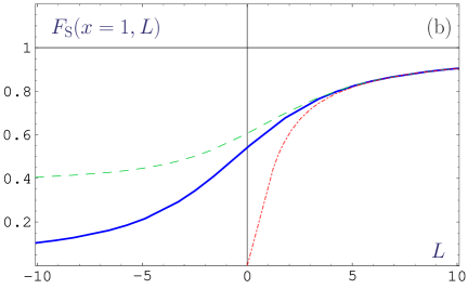
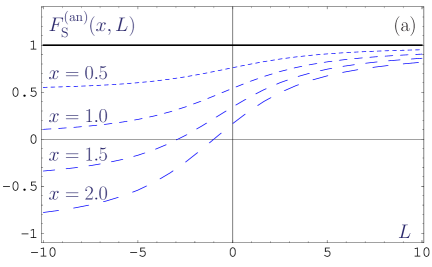
Figure 6: (a) Functions FS(an)(x,L)superscriptsubscript𝐹S(an)𝑥𝐿F_{\text{S}}^{\text{(an)}}(x,L) calculated for different values of x𝑥x using the one-loop FAPT. The horizontal solid line corresponds to x=0𝑥0x=0, while the broken lines represent the specific x𝑥x values shown above them. (b) Comparison of the toy Sudakov function, calculated within the present framework (solid line), with the result of the naive “analytization” SSK99 ; SSK00 ; BPSS04 (dashed line), and that from conventional QCD perturbation theory (dotted line). Note the different scale for the ordinate relative to panel (a).

Here we discuss the analytic image of expression FS(x,L)exp[xa(l)(L)]subscript𝐹S𝑥𝐿𝑥subscript𝑎𝑙𝐿F_{\text{S}}(x,L)\equiv\exp{\left[-x\,a_{(l)}(L)\right]}, which originates as a part of the procedure of the Sudakov resummation, where x𝑥x is a free parameter. We consider the following example, serving as a “toy model” for this resummation:

{FS(x,L)}an{1+m=1[xa(l)(L)]mm!}an=1+m=1(x)m𝒜m(l)(L)m!.subscriptsubscript𝐹S𝑥𝐿ansubscript1subscript𝑚1superscriptdelimited-[]𝑥subscript𝑎𝑙𝐿𝑚𝑚an1subscript𝑚1superscript𝑥𝑚superscriptsubscript𝒜𝑚𝑙𝐿𝑚\displaystyle\left\{F_{\text{S}}(x,L)\right\}_{\rm an}\equiv\left\{1+\sum_{m=1}\frac{\left[-x\,a_{(l)}(L)\right]^{m}}{m!}\right\}_{\rm an}=1+\sum_{m=1}(-x)^{m}\,\frac{{\cal A}_{m}^{(l)}(L)}{m!}\,. (83)

One can verify that for the asymptotic limits of L𝐿L, Eq. (83) reduces to the evident forms:

1+m=1(x)m𝒜m(l)(L)m!=1subscript𝑚1superscript𝑥𝑚superscriptsubscript𝒜𝑚𝑙𝐿𝑚absent\displaystyle 1+\sum_{m=1}(-x)^{m}~{}\frac{{\cal A}_{m}^{(l)}(L)}{m!}= {1xforL;1forL+.cases1𝑥for𝐿1for𝐿\displaystyle\left\{\begin{array}[]{ccl}1-x&~{}\text{for}{}&~{}L\to-\infty\,;\\ 1&~{}\text{for}{}&~{}L\to+\infty\,.\end{array}\right. (86)

The first asymptote on the RHS of Eq. (86) appears due to the equality 𝒜m(l)()=δ1msuperscriptsubscript𝒜𝑚𝑙subscript𝛿1𝑚{\cal A}_{m}^{(l)}(-\infty)=\delta_{1\,m}, see, for instance, Shi98 . The second asymptote is due to the property that in the UV regime APT reduces to the standard perturbation theory. Both properties are illustrated in Fig. 6(a). In Fig. 6(b) we compare different versions of the toy Sudakov function, obtained within the present framework (solid line), using the naive “analytization” SSK99 ; SSK00 ; BPSS04 (dashed line), and conventional QCD perturbation theory (dotted line).

On the other hand, restricting the loop order to l=1𝑙1l=1, one can derive an explicit expression for Eq. (83) in the region of L>0𝐿0L>0, which is based on the Laplace representation given by Eq. (20) and expression (25) for 𝒜~1subscript~𝒜1\tilde{{\cal A}}_{1}, namely,

FS(an)(x,L)=ex/L+xm=1eLmJ1(2xm)m,L>0.formulae-sequencesuperscriptsubscript𝐹S(an)𝑥𝐿superscript𝑒𝑥𝐿𝑥subscript𝑚1superscript𝑒𝐿𝑚subscript𝐽12𝑥𝑚𝑚𝐿0\displaystyle F_{\text{S}}^{\text{(an)}}(x,L)=e^{-x/L}+\sqrt{x}\sum_{m=1}e^{-L\,m}\,\frac{J_{1}(2\sqrt{xm})}{\sqrt{m}},\quad L>0. (87)

The perturbative part of 𝒜~msubscript~𝒜𝑚\tilde{{\cal A}}_{m} in (83) reproduces exactly the asymptotic expression exp[xa(1)(L)]𝑥subscript𝑎1𝐿\exp\left[-x\,a_{(1)}(L)\right] on the RHS of Eq. (87), while the pole remover generates the sum of the exponents in L𝐿-L, weighted by the Bessel functions, J1subscript𝐽1J_{1}, exhibiting how the large L𝐿L behavior is violated.

References

  • (1) S. J. Brodsky, G. P. Lepage, and P. B. Mackenzie, Phys. Rev. D28, 228 (1983).
  • (2) A. P. Bakulev, K. Passek-Kumerički, W. Schroers, and N. G. Stefanis, Phys. Rev. D70, 033014 (2004); [Erratum-ibid. D70, 079906 (2004)].
  • (3) D. V. Shirkov and I. L. Solovtsov, Phys. Rev. Lett. 79, 1209 (1997).
  • (4) D. V. Shirkov, Theor. Math. Phys. 119, 438 (1999).
  • (5) I. L. Solovtsov and D. V. Shirkov, Theor. Math. Phys. 120, 1220 (1999).
  • (6) D. V. Shirkov, Eur. Phys. J. C22, 331 (2001).
  • (7) D. V. Shirkov and I. L. Solovtsov, Phys. Part. Nucl. 32S1, 48 (2001).
  • (8) G. Parisi and R. Petronzio, Nucl. Phys. B154, 427 (1979).
  • (9) J. M. Cornwall, Phys. Rev. D26, 1453 (1982).
  • (10) M. B. Gay Ducati, F. Halzen, and A. A. Natale, Phys. Rev. D48, 2324 (1993).
  • (11) A. C. Mattingly and P. M. Stevenson, Phys. Rev. Lett. 69, 1320 (1992).
  • (12) A. C. Mattingly and P. M. Stevenson, Phys. Rev. D49, 437 (1994).
  • (13) D. V. Shirkov, hep-ph/0003242 (unpublished).
  • (14) D. V. Shirkov, hep-ph/0009106 (unpublished).
  • (15) D. V. Shirkov, hep-ph/0408272 (unpublished).
  • (16) I. L. Solovtsov and D. V. Shirkov, Phys. Lett. B442, 344 (1998).
  • (17) A. P. Bakulev, A. V. Radyushkin, and N. G. Stefanis, Phys. Rev. D62, 113001 (2000).
  • (18) G. Grunberg, hep-ph/9705290 (unpublished).
  • (19) E. Gardi, G. Grunberg, and M. Karliner, JHEP 07, 007 (1998).
  • (20) B. A. Magradze, Int. J. Mod. Phys. A15, 2715 (2000).
  • (21) D. S. Kourashev and B. A. Magradze, hep-ph/0104142 (unpublished).
  • (22) D. S. Kurashev and B. A. Magradze, Theor. Math. Phys. 135, 531 (2003).
  • (23) B. A. Magradze, hep-ph/0305020 (unpublished).
  • (24) A. V. Radyushkin, JINR Rapid Commun. 78, 96 (1996).
  • (25) N. V. Krasnikov and A. A. Pivovarov, Phys. Lett. B116, 168 (1982).
  • (26) H. Contopanagos and G. Sterman, Nucl. Phys. B419, 77 (1994).
  • (27) M. Beneke and V. M. Braun, Phys. Lett. B348, 513 (1995).
  • (28) P. Ball, M. Beneke, and V. M. Braun, Nucl. Phys. B452, 563 (1995).
  • (29) Y. L. Dokshitzer, G. Marchesini, and B. R. Webber, Nucl. Phys. B469, 93 (1996).
  • (30) S. Catani, M. L. Mangano, P. Nason, and L. Trentadue, Nucl. Phys. B478, 273 (1996).
  • (31) L. Magnea, Nucl. Phys. B593, 269 (2001).
  • (32) E. Gardi, Nucl. Phys. B622, 365 (2002).
  • (33) A. V. Nesterenko, Int. J. Mod. Phys. A18, 5475 (2003).
  • (34) A. V. Nesterenko and J. Papavassiliou, Phys. Rev. D71, 016009 (2005).
  • (35) A. C. Aguilar, A. V. Nesterenko, and J. Papavassiliou, J. Phys. G31, 997 (2005).
  • (36) N. G. Stefanis, W. Schroers, and H.-C. Kim, Phys. Lett. B449, 299 (1999).
  • (37) N. G. Stefanis, W. Schroers, and H.-C. Kim, Eur. Phys. J. C18, 137 (2000).
  • (38) A. I. Karanikas and N. G. Stefanis, Phys. Lett. B504, 225 (2001).
  • (39) N. G. Stefanis, Lect. Notes Phys. 616, 153 (2003).
  • (40) A. P. Bakulev, A. I. Karanikas, and N. G. Stefanis, Phys. Rev. D72, 074015 (2005).
  • (41) K. A. Milton and I. L. Solovtsov, Phys. Rev. D55, 5295 (1997).
  • (42) A. Schmedding and O. Yakovlev, Phys. Rev. D62, 116002 (2000).
  • (43) A. P. Bakulev, S. V. Mikhailov, and N. G. Stefanis, Phys. Rev. D67, 074012 (2003).
  • (44) N. N. Bogolyubov, A. A. Logunov, and D. V. Shirkov, Soviet Physics JETP 37, 574 (1960).
  • (45) R. Oehme, Phys. Lett. B252, 641 (1990).
  • (46) B. A. Magradze, hep-ph/0010070 (unpublished).
  • (47) H. Batemann and A. Erdelýi, Higher transcendental functions (Batemann Manuscript Project) (McGraw-Hill, New York, 1953).
  • (48) F. Olver, Asymptotics and special functions (Academic Press, New York, 1974).
  • (49) S. V. Mikhailov, hep-ph/0411397 (unpublished).
  • (50) A. P. Bakulev, S. V. Mikhailov, and N. G. Stefanis, Phys. Lett. 578, 91 (2004).
  • (51) A. P. Bakulev, S. V. Mikhailov, and N. G. Stefanis, Phys. Lett. B508, 279 (2001).
  • (52) E. T. Whittaker and G. N. Watson, A course of modern analysis (Uni. Press, Cambridge, 1927).
  • (53) D. V. Shirkov, Theor. Math. Phys. 127, 409 (2001).
  • (54) D. J. Broadhurst, A. L. Kataev, and C. J. Maxwell, Nucl. Phys. B592, 247 (2001).