Testing the dynamics of $B\rightarrow\pi\pi$ and constraints on $\alpha$

Abstract

In charmless nonleptonic $B$ decays to $\pi\pi$ or $\rho\rho$, the “color allowed” and “color suppressed” tree amplitudes can be studied in a systematic expansion in $\alpha_{s}(m_{b})$ and $\mathchar 28931\relax_{\mathrm{QCD}}/m_{b}$. At leading order in this expansion their relative strong phase vanishes. The implications of this prediction are obscured by penguin contributions. We propose to use this prediction to test the relative importance of the various penguin amplitudes using experimental data. The present $B\rightarrow\pi\pi$ data suggest that there are large corrections to the heavy quark limit, which can be due to power corrections to the tree amplitudes, large up-penguin amplitude, or enhanced weak annihilation. Because the penguin contributions are smaller, the heavy quark limit is more consistent with the $B\rightarrow\rho\rho$ data, and its implications may become important for the extraction of $\alpha$ from this mode in the future.

I Introduction

Nonleptonic $B$ decays to light hadrons provide information about $C\!P$ violation. In particular, the decays to $\pi\pi$, $\rho\pi$ and $\rho\rho$ can determine the weak phase $\alpha$. The theoretical challenge is to disentangle the strong interaction physics from the weak phase one would like to determine. For the decay $B^{0}\rightarrow\pi^{+}\pi^{-}$ the $B$ factories study the $C\!P$ asymmetry,

$$\frac{\Gamma[\kern 1.79993pt\overline{\kern-1.79993ptB}{}^{0}(t)\rightarrow\pi^{+}\pi^{-}]-\Gamma[B^{0}(t)\rightarrow\pi^{+}\pi^{-}]}{\Gamma[\kern 1.79993pt\overline{\kern-1.79993ptB}{}^{0}(t)\rightarrow\pi^{+}\pi^{-}]+\Gamma[B^{0}(t)\rightarrow\pi^{+}\pi^{-}]}$$ (1)

$$\hskip 14.22636pt=S_{+-}\sin(\Delta m\,t)-C_{+-}\cos(\Delta m\,t)\,,$$

with the present world averages pipiCP ; Group:2004cx

$$S_{+-}=-0.50\pm 0.12,\qquad C_{+-}=-0.37\pm 0.10\,.$$ (2)

If the $B\rightarrow\pi^{+}\pi^{-}$ amplitude were dominated by contributions with a single weak phase, the observable

$$\sin(2\alpha_{\rm eff})=S_{+-}\big{/}\sqrt{1-C_{+-}^{2}}\,,$$ (3)

would be equal to $\sin 2\alpha$ and $C_{+-}$ would be zero. The data indicate that this is not a good approximation. An isospin analysis Gronau:1990ka still allows a theoretically clean determination of $\alpha$ if the $B^{0}\rightarrow\pi^{0}\pi^{0}$ and $\kern 1.79993pt\overline{\kern-1.79993ptB}{}^{0}\rightarrow\pi^{0}\pi^{0}$ rates are precisely measured. Since this requires very large data samples, several strategies have been proposed to extract $\alpha$ from $\alpha_{\rm eff}$ relying on theoretical inputs.

In the last few years the theory of $B\rightarrow\pi\pi$ decays has advanced considerably. Using the heavy quark limit, factorization theorems have been proven for the decay amplitudes at leading order in $\mathchar 28931\relax/m_{b}$. The amplitudes in Eq. (I) arise from the matrix element of the effective Hamiltonian,

$$H_{\rm eff}=-{4G_{F}\over\sqrt{2}}\bigg{[}\lambda_{u}\Big{(}C_{1}O_{1}^{u}+C_{2}O_{2}^{u}+\sum_{i\geq 3}C_{i}^{c}O_{i}\Big{)}$$

$${}\qquad\ +\lambda_{c}\Big{(}C_{1}O_{1}^{c}+C_{2}O_{2}^{c}+\sum_{i\geq 3}C_{i}^{c}O_{i}\Big{)}$$

$${}\qquad\ +\lambda_{t}\,\sum_{i\geq 3}C_{i}^{t}\,O_{i}\bigg{]}\,,$$ (4)

where CKM-unitarity was not used, and $i=3,\ldots,6,8$. (In the usual notation one has $C_{i}=C_{i}^{c}-C_{i}^{t}$.) Its $\kern 1.79993pt\overline{\kern-1.79993ptB}{}\rightarrow\pi\pi$ matrix element can be parameterized as

$$\kern 1.79993pt\overline{\kern-1.79993ptA}{}(\kern 1.79993pt\overline{\kern-1.79993ptB}{}^{0}\rightarrow\pi^{+}\pi^{-}) = -\lambda_{u}(T+P_{u})-\lambda_{c}P_{c}-\lambda_{t}P_{t}$$

$$= e^{-i\gamma}T_{\pi\pi}+e^{i\phi}P_{\pi\pi}\,,$$

$$\sqrt{2}\kern 1.79993pt\overline{\kern-1.79993ptA}{}(\kern 1.79993pt\overline{\kern-1.79993ptB}{}^{0}\rightarrow\pi^{0}\pi^{0}) = \lambda_{u}(-C+P_{u})+\lambda_{c}P_{c}+\lambda_{t}P_{t}$$

$$= e^{-i\gamma}C_{\pi\pi}-e^{i\phi}P_{\pi\pi}\,,$$

$$\sqrt{2}\kern 1.79993pt\overline{\kern-1.79993ptA}{}(B^{-}\rightarrow\pi^{-}\pi^{0}) = -\lambda_{u}(T+C)=e^{-i\gamma}T_{-0}\,,$$ (5)

where $\lambda_{q}=V_{qb}V_{qd}^{*}$. (We neglect isospin breaking isospinbreak and the contributions of electroweak penguins, the dominant part of which can be included model independently ewp .) In Eq. (I) $T+P_{u}$ and $C-P_{u}$ are the $B\rightarrow\pi^{+}\pi^{-}$ and $B\rightarrow\pi^{0}\pi^{0}$ matrix elements of the terms in the first line in Eq. (I), while $P_{c}$ and $P_{t}$ are the matrix elements of the second and third lines, respectively. This implies that each of the $T+P_{u}$, $C-P_{u}$, $P_{c}$ and $P_{t}$ terms are separately renormalization group invariant.

There is an ambiguity in Eq. (I) related to the freedom in choosing the weak phase $\phi$, in terms of which the amplitudes are written. There are two widely used conventions corresponding to eliminating either $\lambda_{t}$ or $\lambda_{c}$ using unitarity (some aspects of this were discussed in Refs. conv ). In the t-convention one eliminates $\lambda_{t}$ from Eq. (I), while in the c-convention one eliminates $\lambda_{c}$. Table 1 shows the expressions for the amplitudes and $\phi$ in these conventions. Once a choice is made, $T_{\pi\pi}$, $C_{\pi\pi}$, $P_{\pi\pi}$, and $T_{-0}$ can be extracted from the data, while further theoretical input is needed to determine $T$, $C$ and $P_{u,c,t}$.

The amplitudes in Eq. (I) (and their $C\!P$ conjugates) satisfy the isospin relation

$$\frac{1}{\sqrt{2}}\kern 1.79993pt\overline{\kern-1.79993ptA}{}(\kern 1.79993pt\overline{\kern-1.79993ptB}{}^{0}\rightarrow\pi^{+}\pi^{-})+\kern 1.79993pt\overline{\kern-1.79993ptA}{}(\kern 1.79993pt\overline{\kern-1.79993ptB}{}^{0}\rightarrow\pi^{0}\pi^{0})=\kern 1.79993pt\overline{\kern-1.79993ptA}{}(B^{-}\rightarrow\pi^{-}\pi^{0})\,.$$ (6)

The “tree” amplitudes also satisfy the relation

$$T_{\pi\pi}+C_{\pi\pi}=T_{-0}\,,$$ (7)

which will play an important role in this paper, and we refer to it as the “tree triangle” (TT).

Expanding the amplitudes in soft-collinear effective theory (SCET) scet , one can define the leading (in $\mathchar 28931\relax/m_{b}$) parts of $T$, $C$, and $P_{u}$ separately in terms of matrix elements of distinct SCET operators bp , which we denote with $(0)$ superscripts. The relative strong phase of $T^{(0)}$ and $C^{(0)}$ is suppressed by $\alpha_{s}$ bprs ; qcdf , and therefore

$$\phi_{T}\equiv\arg\bigg{(}{T^{(0)}+P_{u}^{(0)}\over T+C}\bigg{)}={\cal O}\big{[}\alpha_{s}(m_{b}),\,\mathchar 28931\relax_{\mathrm{QCD}}/m_{b}\big{]}\,.$$ (8)

The numerator includes $P_{u}^{(0)}$ so that $\phi_{T}$ is scale independent. The denominator could be defined to contain $T^{(0)}+C^{(0)}$, and our choice is for later convenience. Neither of these affect the right-hand side of Eq. (8) [recall: $P_{u}^{(0)}/T^{(0)}={\cal O}(\alpha_{s})$]. We define $T^{\prime(0)}\equiv T^{(0)}+P_{u}^{(0)}$ and $T+P_{u}\equiv T^{\prime(0)}+P_{u}^{\prime}$, and in the rest of this paper the primes will be dropped. Thus, hereafter, $P_{u}$ contains the power suppressed corrections to $T+P_{u}$ (including weak annihilation).

Table 1: The $B\rightarrow\pi\pi$ amplitudes and the phase of the penguin amplitude in the c- and t-conventions ($P_{ij}\equiv P_{i}-P_{j}$).

amplitude	t-convention	c-convention
$T_{\pi\pi}$	$|\lambda_{u}|(-T-P_{ut})$	$|\lambda_{u}|(-T-P_{uc})$
$C_{\pi\pi}$	$|\lambda_{u}|(-C+P_{ut})$	$|\lambda_{u}|(-C+P_{uc})$
$P_{\pi\pi}$	$-|\lambda_{c}|P_{ct}$	$|\lambda_{t}|P_{ct}$
$\phi$	$\pi$	$\beta$

The implications of Eq. (8) for the determination of $\alpha$ are obscured by the fact that $T$ and $C$ are not directly observable. The amplitudes $T_{\pi\pi}$ and $C_{\pi\pi}$ in Eq. (I) that can be extracted from the data include contributions from $P_{u,c,t}$. The heavy quark limit also determines the power counting for the penguin amplitudes, however, the convergence of the expansion for the penguins is less clear than it is for the trees. At leading order in $\mathchar 28931\relax/m_{b}$ the calculable parts of $P_{u,c,t}$ are suppressed by $\alpha_{s}$ or the small Wilson coefficients $C_{3,4}$. At subleading order, the QCD factorization (QCDF) formula for $P_{t}$ contains sizeable “chirally enhanced” corrections, comparable to the leading order term qcdf . The possible size of nonperturbative contributions to $P_{c}$ has also been the subject of debate bprs ; pcdedbate . A large $P_{c}$ amplitude was found in fits using the leading order factorization results in SCET bprs , or adding a free parameter to the leading order QCDF result cpengs . In QCDF $P_{c}$ is claimed to be computable at leading order without nonperturbative inputs, while $P_{t}$ receives sizable “chirally enhanced” ${\cal O}(\mathchar 28931\relax/m_{b})$ corrections. Equation (8) and allowing for large long distance contribution to $P_{c}$ was used in Ref. brs to determine $\alpha$ without using the measurement of $C_{00}$ (the direct $C\!P$ asymmetry in $B\rightarrow\pi^{0}\pi^{0}$).

The penguin amplitudes $P_{c}$ and $P_{t}$ introduce a difference between the TTs in the two conventions. The $P_{u}$ amplitude is common to $T_{\pi\pi}$ in the t- and c-conventions, but $P_{c}$ enters $T_{\pi\pi}$ in the c-convention and $P_{t}$ enters $T_{\pi\pi}$ in the t-convention. Understanding the relative hierarchy of the three penguin amplitudes, $P_{u,c,t}$, is important if one is to use Eq. (8) for the determination of $\alpha$. In addition, it may also shed light on the $\mathchar 28931\relax/m_{b}$ power counting for the penguin amplitudes. In this paper we show that by comparing the shapes of the TT in the c and t-conventions we can gain empirical knowledge about the relative sizes of $P_{u}$, $P_{c}$ and $P_{t}$.

II Isospin analysis and tree triangle

The isospin relation in Eq. (6) holds for both the $\kern 1.79993pt\overline{\kern-1.79993ptB}{}$ and $B$ decay amplitudes, denoted by $\bar{A}$ and $A$, respectively. It is convenient to define $\widetilde{A}^{ij}=e^{2i\gamma}\kern 1.79993pt\overline{\kern-1.79993ptA}{}^{ij}$, so that $A^{0+}=\widetilde{A}^{0-}$. Figure 1 shows the resulting two isospin triangles, $WZX$ and $WZY$, where the tree triangle, $WZV$, is also drawn. We follow the notation of Ref. GLSS , but normalize $A(B^{+}\rightarrow\pi^{0}\pi^{+})=\overline{WZ}=1$.

Figure 1: Isospin triangles for $\kern 1.79993pt\overline{\kern-1.79993ptB}{}$ and $B$ decay, $WZY$ and $WZX$. $WVZ$ is the tree triangle (TT), Eq. (7), with $WV=T_{\pi\pi}$ and $ZV=C_{\pi\pi}$. The dashed lines show the $P_{\pi\pi}$ amplitudes.

To determine the TT from the data, recall that the $WZX$ and $WZY$ isospin triangles can be obtained from the direct $C\!P$ asymmetries $C_{+-}$ and $C_{00}$, and the ratios of branching fractions

$$R_{+-} = \frac{{\cal B}(B^{0}\rightarrow\pi^{+}\pi^{-})}{2\,{\cal B}(B^{+}\rightarrow\pi^{+}\pi^{0})}\,\frac{\tau_{B^{+}}}{\tau_{B^{0}}}=0.44^{\,+0.07}_{\,-0.06}\,,$$

$$R_{00} = \frac{{\cal B}(B^{0}\rightarrow\pi^{0}\pi^{0})}{{\cal B}(B^{+}\rightarrow\pi^{+}\pi^{0})}\,\frac{\tau_{B^{+}}}{\tau_{B^{0}}}=0.29^{\,+0.07}_{\,-0.06}\,,$$ (9)

where we used the experimental inputs from pipiBr ; Group:2004cx . Taking the ratios eliminates an arbitrary overall normalization parameter. To determine the coordinates of $V$, however, the measurement of $S_{+-}$ is also needed.

It is convenient to define the coordinates of $X$ and $Y$ to be $(\pm\ell,0)$, with

$$\ell^{2}=\frac{1}{2}R_{+-}\Big{[}1-\sqrt{1-C_{+-}^{2}}\cos 2\Delta\alpha\Big{]},$$ (10)

where $\Delta\alpha\equiv\alpha-\alpha_{\rm eff}$ and $\alpha_{\rm eff}$ is defined in Eq. (3). The four coordinates of $W$ and $Z$ and the phase $\Delta\alpha$ are given by the solutions of the five equations GLSS

$$1 = (x_{Z}-x_{W})^{2}+(y_{Z}-y_{W})^{2},$$

$$R_{00} = x_{Z}^{2}+y_{Z}^{2}+\ell^{2},$$

$$R_{+-} = x_{W}^{2}+y_{W}^{2}+\ell^{2},$$

$$R_{+-}C_{+-} = -2\ell x_{W},$$

$$R_{00}C_{00} = -2\ell x_{Z}.$$ (11)

The $XVY$ angle is $2(\phi+\gamma)$, so that the $y$ coordinate of $V\,(0,y_{V})$ is

$$y_{V}=\cases{-\ell\cot\gamma\,,&\mbox{in the t-convention}\,,\cr{\phantom{-}}\ell\cot\alpha\,,&\mbox{in the c-convention}\,.\cr}$$ (12)

Equations (II) can be solved for $\Delta\alpha$ and the coordinates of $W$ and $Z$. Because of the relative orientation of the amplitudes $A^{+-}$ and $\widetilde{A}^{+-}$ adopted in Fig. 1, the solution must also satisfy $\mbox{sgn}(\Delta\alpha)=\mbox{sgn}(y_{W})$.

Some important properties of the solutions are apparent. First, $x_{W}=0$ if and only if $C_{+-}=0$ (similarly, $x_{Z}=0$ if and only if $C_{00}=0$). Second, the sign of $x_{W}$ ($x_{Z}$) is opposite of that of $C_{+-}$ ($C_{00}$). Thus, $WZ$ crosses the $y$ axis if and only if the direct $C\!P$ asymmetries in the charged and neutral modes have opposite signs.

In the rest of this section, we treat the simplified case where $C_{00}$ is not known. The first four equations in (II) can be used to solve for the coordinates of $W$ and $Z$ as functions of $\Delta\alpha$. For any given value of $\Delta\alpha$, $W$ and $Z$ are determined up to a two-fold ambiguity, corresponding to the reflection of $Z$ about the $WO$ line. These equations also place bounds on $\ell$ and $\Delta\alpha$ Grossman:1997jr ; GLSS

$$\ell^{2} \leq R_{+-}R_{00}-{(1-R_{+-}-R_{00})^{2}\over 4}\,,$$

$$\cos(2\Delta\alpha) \geq {(1+R_{+-}-R_{00})^{2}-2R_{+-}\over 2R_{+-}\sqrt{1-C_{+-}^{2}}}\,.$$ (13)

We refer to these inequalities as the isospin bound, and define $\alpha_{\rm bound}\equiv\alpha_{\rm eff}\pm\Delta\alpha_{\rm max}$, which can be obtained from Eqs. (3) and (II), and $\gamma_{\rm bound}\equiv\pi-\beta-\alpha_{\rm bound}$. (Here, and in what follows $\beta$ is treated as known.) The coordinates of $W$ and $Z$ at the isospin bound satisfy

$${x_{Z}\over x_{W}}\bigg{|}_{\rm bound}={y_{Z}\over y_{W}}\bigg{|}_{\rm bound}=-{1+R_{00}-R_{+-}\over 1-R_{00}+R_{+-}}\,.$$ (14)

This means that at the isospin bound $W$, $Z$, and $O$ are on one line and that at the bound

$$C_{00}\big{|}_{\rm bound}=-{R_{+-}\over R_{00}}\,{1+R_{00}-R_{+-}\over 1-R_{00}+R_{+-}}\;C_{+-}\big{|}_{\rm bound}\,.$$ (15)

The present data gives at the isospin bound $C_{00}=-(1.1\pm 0.1)\,C_{+-}$, which is almost $2\sigma$ from the measurements of $C_{+-}$ in Eq. (2) and $C_{00}=-0.28^{+0.39}_{-0.40}$ c00 ; Group:2004cx .

In general, and even at the isospin bound, the $V$ vertex of the TT depends on $S_{+-}$ via Eq. (12). Thus, the shape of the TT at the bound is not fixed, but depends on the experimental results. This dependence enters through $\alpha_{\rm eff}+\Delta\alpha$ and implies that if one uses a constraint on the shape of the TT to extract $\alpha$, then i) the solution is not invariant under $\Delta\alpha\leftrightarrow-\Delta\alpha$, and ii) the allowed values of $\Delta\alpha$ are not the same for each discrete ambiguity of $\alpha_{\rm eff}$. Both of these points are different from the well-known symmetry properties of the usual isospin analysis.

The theory prediction of a small strong phase in Eq. (8) implies that the TT should be nearly flat, up to penguin contributions, small $\alpha_{s}$ and unknown $\mathchar 28931\relax/m_{b}$ corrections. While the penguin contamination makes the definition of the TT itself convention dependent, it is interesting to consider under what conditions the TT can be flat, and its relation to the isospin bound. Since at the isospin bound $W$, $Z$, and $O$ are on a line, unless $y_{V}=0$, the TT is flat at the isospin bound if and only if $x_{W}=x_{Z}=0$. This implies that if any two of the following statements hold, then the other three follow:

1. The t-convention TT is flat for generic $$\alpha$$;

2. The c-convention TT is flat for generic ;

3. is at the isospin bound;

4. ;

5. .

(16)

Equivalently, when one of the statements in (16) holds, the other four are either all true or all false. This shows that whether the TT is flat near the isospin bound or not depends on the value of $\alpha$; i.e., the TT being flat and $\alpha$ (or $\gamma$) being close to the isospin bound are in principle unrelated.

III Constraints on $\alpha$

In Ref. brs , the predicted smallness of $\phi_{T}$ and $P_{ut}$ was used to imply that the TT in the t-convention is (near) flat, which, in turn, was used to extract $\gamma$ without the insufficiently known $C_{00}$. In this section we discuss the implications of knowing an angle in the TT for the determination of $\alpha$, using a method which makes transparent the dependence of the constraints on $\alpha$ on the data.

For given $R_{+-}$, $R_{00}$, and $C_{+-}$, the first four equations in (II) together with (10) determine the coordinates of $W$ and $Z$ as functions of $\Delta\alpha$. If, in addition, an angle in the TT is also known, then the position of the point $V$ is determined. We find it simplest to discuss the constraints in terms of the (convention dependent) observable phase,

$$\tau^{(q)}\equiv\arg\bigg{(}{T_{\pi\pi}^{(q)}\over T_{-0}}\bigg{)}=\arg\bigg{(}1+{P_{uq}\over T^{(0)}}\bigg{)}+\phi_{T},$$ (17)

where $q=c$ or $t$. The TT is near flat in either convention if $|\tau|\ll 1$. Note that if the penguin amplitudes vanished, then $\tau^{(t)}=\tau^{(c)}=\phi_{T}$. We can determine the coordinates of $V$ as a function of $\Delta\alpha$ in two ways: from the value of $\tau$ and the coordinates of $W$ and $Z$

$$y_{V}(\Delta\alpha)=y_{W}-x_{W}\frac{y_{Z}-y_{W}-(x_{Z}-x_{W})\tan\tau}{x_{Z}-x_{W}+(y_{Z}-y_{W})\tan\tau}\,,$$ (18)

and from Eq. (12) if $\beta$, $S_{+-}$ and $C_{+-}$ are measured

$$y_{V}(\Delta\alpha)=\cases{\ell\,\cot(\beta+\alpha_{\rm eff}+\Delta\alpha)\,,&\mbox{t-convention},\cr\ell\,\cot(\alpha_{\rm eff}+\Delta\alpha)\,,&\mbox{c-convention}.\cr}$$ (19)

The expression in (19) is convention dependent, because so is the definition of $\tau$ that enters in (18). These two equations form an implicit equation for $\Delta\alpha$.

Figure 2 illustrates this method for the central values of the data. The solid curves show the solution for $y_{V}(\Delta\alpha)$ vs. $\Delta\alpha$ from Eq. (19): the darker (blue) curve corresponds to the t-convention and $\alpha_{\rm eff}\simeq 106^{\circ}$, while the lighter (red) curves correspond to the c-convention (the upper one for $\alpha_{\rm eff}\simeq 106^{\circ}$, the lower one for its mirror solution $\alpha_{\rm eff}\simeq 164^{\circ}$). The dashed curve shows $y_{V}$ vs. $\Delta\alpha$ from Eq. (18) for $\tau=0$, and its intersections with the solid curves determine the value of $\Delta\alpha$, which together with $\alpha_{\rm eff}$ gives $\alpha$. For the purpose of illustration the dotted curves show $\tau=+10^{\circ}$ (lower curve) and $-10^{\circ}$ (up-most curve).

Figure 2: The solid curves are $y_{V}$ vs. $\Delta\alpha$ from Eq. (19): the darker (blue) curve corresponds to the t-convention and $\alpha_{\rm eff}\simeq 106^{\circ}$, while the lighter (red) curves to the c-convention (the upper one for $\alpha_{\rm eff}\simeq 106^{\circ}$, the lower one for $\alpha_{\rm eff}\simeq 164^{\circ}$). The dashed curve shows the solution of Eq. (18) for $\tau=0$, and the dotted curves are $\tau=+10^{\circ}$ (lower) and $\tau=-10^{\circ}$ (upper).

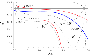
The $\tau=0$ curve goes to $y_{V}=0$ at the isospin bound (see Fig. 2), in accordance with our result in Sec. II that if $\Delta\alpha$ is at the isospin bound and the TT is flat, then $y_{V}=0$. The right-hand side of Eq. (19) is small in this region of $\Delta\alpha$, since the argument of the cotangent is close to $90^{\circ}$ (the central values of the $\pi\pi$ data give $\alpha_{\rm eff}\simeq 106^{\circ}$, so that at the smallest value of $\Delta\alpha\simeq-28^{\circ}$, $\beta+\alpha_{\rm eff}+\Delta\alpha\simeq 102^{\circ}$ and $\alpha_{\rm eff}+\Delta\alpha\simeq 79^{\circ}$). These two facts imply that there is a solution for $\Delta\alpha$ near the isospin bound with a flat TT; however, this is a coincidence and not a necessity.

In Ref. brs it was found that for small $\tau^{(t)}$ the solution for $\Delta\alpha$ was close to the isospin bound. This can be easily seen from Fig. 2. The dashed and dotted curves are steep near the bound for negative $\Delta\alpha$, so changing $\tau$ hardly changes the solution for $\Delta\alpha$. However, for the other solution (corresponding to positive $\Delta\alpha$, and a value of $\alpha$ disfavored by the global CKM fit Charles:2004jd ), the error is significantly larger, since the dependence of $\Delta\alpha$ on $\tau$ is stronger. The allowed region of $\Delta\alpha$ is particularly sensitive to $R_{00}$; for example, for $R_{00}=0.2$ (which is a bit more than $1\sigma$ lower than its present central value) the $|\tau|<10^{\circ}$ constraint would include almost all values of $\Delta\alpha$ that are allowed by the isospin analysis. Note that with the current data the error of $\alpha$ extracted using the constraint of a small $\tau$ increases with decreasing $R_{00}$, contrary to the isospin analysis.

Figure 3: Left plot: confidence level for $\alpha$ imposing $\tau=0$ in the t- (solid line) and c-conventions (dashed line) without using $C_{00}$ in the fit. The t-convention curve uses $\beta$ as an input. Also shown are the results of the traditional isospin analysis Gronau:1990ka ; Charles:2004jd with (light shaded region) and without (dark shaded region) using $C_{00}$. The dot with $1\sigma$ error bar shows the predicton from the global CKM fit (not including the direct measurement of $\alpha$) Charles:2004jd . Right plot: confidence level for $\alpha$ imposing $\tau=0$ in the t-convention with (dotted line) and without (solid line) using the $C_{00}$ result in the fit. Also shown are the constraints in the t-convention imposing $|\tau|<5^{\circ}$, $|\tau|<10^{\circ}$, and $|\tau|<20^{\circ}$ (dashed lines). The shaded region is the same as in the left plot.

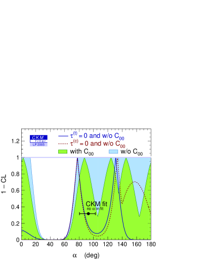
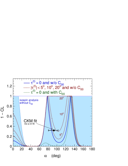
The confidence level (CL) of $\alpha$ obtained by imposing a constraint on $\tau$ is shown in Fig. 3 using the CKMfitter package Charles:2004jd . In the left plot the curves show (see the labels) the CL of $\alpha$ imposing $\tau=0$ in both the t- and c-conventions without using the $C_{00}$ measurement in the fit. For comparison, we also show the result of the usual isospin analysis with and without using $C_{00}$. The plot on the right-hand side shows the CL of $\alpha$ imposing $\tau=0$ in the t-convention with and without using $C_{00}$, and the constraint in the t-convention imposing $|\tau|<5^{\circ}$, $10^{\circ}$, and $20^{\circ}$. The restriction on $\alpha$ from a constraint $|\tau|<\tau_{0}$ becomes quite weak as $\tau_{0}$ increases in the range $10^{\circ}<\tau_{0}<20^{\circ}$. We can compare our results with those of brs , which use as theory input an upper bound on $\epsilon=|{\rm Im}(C^{(t)}_{\pi\pi}/T^{(t)}_{\pi\pi})|$. Assuming $\{\gamma,|\arg(P_{\pi\pi}/T_{\pi\pi})|\}<90^{\circ}$, we find $\sin\tau^{(t)}<\epsilon\,\sqrt{R_{+-}}$, i.e., $\tau^{(t)}<15.5^{\circ}\ (7.8^{\circ})$ for the bounds considered in brs , $\epsilon<0.4\ (0.2)$.

Imposing $\tau=0$ gives only two solutions with $\chi^{2}=0$ with the current data, around $\alpha\sim 78^{\circ}$ and $132^{\circ}$. The first one, which is consistent with the Standard Model (SM) CKM fit, is disfavored by the measurement of $C_{00}$. While the two solutions have comparable errors for $\tau=0$, allowing a finite range of $\tau$ to account for subleading effects increases the error of the $\alpha\sim 132^{\circ}$ solution more rapidly. Imposing a bound on $|{\rm Im}(C/T)|$ brs allows, in addition to $\tau$ being near 0, that $\tau$ is near $\pi$ (mod $2\pi$); however, the theory disfavors the latter possibility. It is constraining $|\tau|$ modulo $2\pi$ and not $\pi$ that makes some of the CL curves not periodic with a period of $\pi$.

These results for $\alpha$ should not be taken at face value, because in the next Section we find that extracting $\tau$ using the SM CKM fit as an input gives significantly larger values of $|\tau|$ than considered here. The implications of this are discussed below.

IV The penguin hierarchy problem

If the penguin amplitudes were small then the statements in (16) would all hold to a good precision, and $\alpha$ could be extracted simply from $S_{+-}$. This is known not to be the case, so the question is to determine which penguins are large or small. This is complicated by the fact that, as explained in Sec. II, the amplitudes $T$, $C$, $P_{uc}$, and $P_{ut}$ are not separately observable from the $B\rightarrow\pi\pi$ data alone. They can be disentangled using $SU(3)$ flavor symmetry and data on $B\rightarrow K\pi$, $K\kern 1.99997pt\overline{\kern-1.99997ptK}{}$, etc.

In this section we propose to use the theory expectation for $\phi_{T}$ in Eq. (8) to test the magnitude of the penguins. (Another test of corrections to factorization in $B\rightarrow\pi\pi$ was proposed in Feldmann:2004mg .) We assume $\phi_{T}=0$, although we may learn from other data that power corrections to tree amplitudes are sizable. For example, a power suppressed strong phase around $30^{\circ}$ is observed in $B\rightarrow D\pi$ decays Mantry:2003uz .

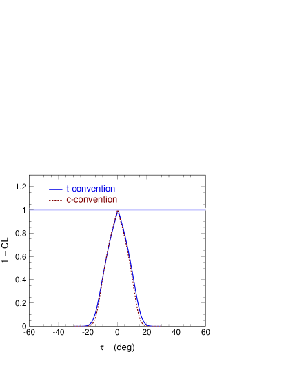
In the t-convention $P_{ut}$ (recall, $P_{ij}\equiv P_{i}-P_{j}$) contributes to the TT in Eq. (7), while in the c-convention it is $P_{uc}$. (We choose, for convenience, the pure tree amplitude $T_{-0}$ to be real.) Thus, comparing the TT in the two conventions teaches us about the relative size of $P_{ut}$ and $P_{uc}$. (The same information can in principle be obtained from the fit in any one convention; this comparison makes the results more transparent.) We use the SM global fit to the CKM matrix that determines the weak phase $\gamma=(59.0^{+6.4}_{-4.9})^{\circ}$ Charles:2004jd . This allows the construction of the tree triangles in both conventions, as explained in Sec. II. Comparing how flat they are, i.e., how small the angle $\tau$ of the TT is, the following outcomes are possible:

Figure 4: Confidence level plots for $\tau=\arg(T_{\pi\pi}/T_{-0})$ in the t- and c-conventions in $\kern 1.79993pt\overline{\kern-1.79993ptB}{}\rightarrow\pi\pi$ (left), and for $\kern 1.79993pt\overline{\kern-1.79993ptB}{}\rightarrow\rho\rho$ (right).

• $|\tau^{(t)}|\ll|\tau^{(c)}|$. This would imply ${\rm Im}(P_{ut})\ll{\rm Im}(P_{uc})$, and the likely explanation would be $|P_{c}|\gg|P_{u}|\sim|P_{t}|$.

• $|\tau^{(t)}|\gg|\tau^{(c)}|$. This would imply ${\rm Im}(P_{ut})\gg{\rm Im}(P_{uc})$, and the likely explanation would be $|P_{t}|\gg|P_{u}|\sim|P_{c}|$.

• $|\tau^{(t)}|\sim|\tau^{(c)}|\ll 1$. This would imply that both ${\rm Im}(P_{ut}/T^{(0)})$ and ${\rm Im}(P_{uc}/T^{(0)})$ are small. In this case the likely explanation would be that $P_{q}/T^{(0)}$ is small for each of the penguin amplitudes.

• $|\tau^{(t)}|\sim|\tau^{(c)}|={\cal O}(1)$ and $|\tau^{(t)}-\tau^{(c)}|\ll 1$. This would imply that ${\rm Im}(P_{ut}/T^{(0)})$ and ${\rm Im}(P_{uc}/T^{(0)})$ are both much larger than ${\rm Im}(P_{ct}/T^{(0)})$. There appears to be no single plausible explanation for such a case. It may indicate that $P_{u}$ (that includes weak annihilation) is large, while $P_{c}$ and $P_{t}$ are small or have small phases. Another, fine tuned, possibility is that both $P_{c}$ and $P_{t}$ have large but nearly equal phases. Last, it might be that $\phi_{T}={\cal O}(1)$, indicating large corrections to the heavy quark limit.

• $|\tau^{(t)}|\sim|\tau^{(c)}|={\cal O}(1)$ and $|\tau^{(t)}-\tau^{(c)}|={\cal O}(1)$. This would imply that ${\rm Im}(P_{ut}/T^{(0)})$, ${\rm Im}(P_{uc}/T^{(0)})$, and ${\rm Im}(P_{ct}/T^{(0)})$ are all large. In this case the likely explanation would be that all penguins are large and comparable to $T^{(0)}$.

Note that the $\tau^{(t)}-\tau^{(c)}$ difference is related to the penguin-to-tree ratio,

$$\tau^{(t)}-\tau^{(c)}=-\arg\bigg{(}1-\frac{|\lambda_{u}|}{|\lambda_{c}|}\,\frac{P_{\pi\pi}^{(t)}}{T_{\pi\pi}^{(t)}}\bigg{)},$$ (20)

and can be determined with better precision than $\tau^{(t,c)}$ separately.

IV.1 $B\rightarrow\pi\pi$

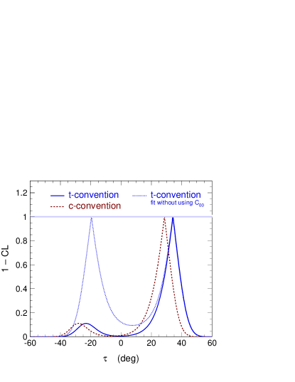
Using the experimental data we can determine $\tau$ in the t- and c-conventions. The results for the confidence levels of $\tau^{(t,c)}$ are shown in the left plot in Fig. 4. At the one sigma level only one solution is allowed (because $C_{00}$ disfavors one of the solutions at a near $2\sigma$ level). Including $C_{00}$ in the fit drives $|\tau|$ to larger values

$$\tau=\cases{\big{(}36^{+6}_{-8}\big{)}^{\circ},&t-convention,\cr\big{(}30^{+6}_{-8}\big{)}^{\circ},&c-convention.\cr}$$ (21)

Note that the central values indicate rather large values for $\tau$ in both conventions. Their difference is more accurately determined by Eq. (20), where the fit gives

$$\tau^{(t)}-\tau^{(c)}=\big{(}5.7^{+2.0}_{-1.7}\big{)}^{\circ}.$$ (22)

Eqs. (21) and (22) favor scenario (iv). While this may have several reasons as explained above, the least fine-tuned one, i.e., a large $P_{u}$ (including weak annihilation) and smaller $P_{c,t}$ penguins (or that the $\phi_{T}\ll 1$ prediction receives large corrections), would be puzzling for any approach to factorization. At present, this is not a very firm conclusion yet. (Note that a similar enhancement of the $u$-penguin amplitude is observed in $\kern 1.79993pt\overline{\kern-1.79993ptB}{}\rightarrow K\pi$ and $b\rightarrow(s\overline{s})s$ decays, if the apparent anomalies therein are interpreted within the SM.)

IV.2 $B\rightarrow\rho\rho$

Since $B\rightarrow\rho\rho$ decays are dominantly longitudinally polarized, the determination of $\alpha$ from this mode is very similar to that from $B\rightarrow\pi\pi$, except that at the few percent level an $I=1$ amplitude may be present Falk:2003uq . Using dynamical input to reduce the uncertainty of $\alpha$ from $B\rightarrow\rho\rho$ has received little attention so far, because the isospin bound puts tight constraints on $\alpha-\alpha_{\rm eff}$. However, this bound may become worse in the future, since the strong present bound is a consequence of the fact that the isospin triangles do not close with the central values of the current world averages. This is a consequence of both the branching ratios, whose central values in units of $10^{-3}$ are $\sqrt{{\cal B}(B\rightarrow\rho^{+}\rho^{0})}=5.14$, $\sqrt{{\cal B}(B\rightarrow\rho^{+}\rho^{-})/2}=3.87$, and $\sqrt{{\cal B}(B\rightarrow\rho^{0}\rho^{0})}<1.05$ (90% CL), and the smallness of $C_{\rho^{+}\rho^{-}}=-0.03\pm 0.20$ Group:2004cx ; rhorho . Therefore, although at present imposing $|\tau|<10^{\circ}$ does not improve the constraint on $\alpha-\alpha_{\rm eff}$ in this mode, such a dynamical input may become useful in the future.

In this case, the $\tau$ values in the two conventions differ by less than a degree as shown in the right plot in Fig. 4, giving $\tau=(0\pm 12)^{\circ}$. This may tend towards the above scenario (iii). If in the future the measured value of the $B\rightarrow\rho^{+}\rho^{0}$ branching ratio decreases (or that of $\rho^{0}\rho^{0}$ increases) then the pure isospin bound will become worse, and the fit results for $\tau$ will also change. If that fit still favors $|\tau^{(t)}|\ll|\tau^{(c)}|$ or $|\tau^{(t)}|\sim|\tau^{(c)}|\ll 1$ [cases (i) or (iii)] then we would feel comfortable imposing a constraint on the magnitude of $\tau^{(t)}$ to improve the determination of the CKM angle $\alpha$.

V Conclusions

The tree amplitudes in $B\rightarrow\pi\pi$ decays can be computed in an expansion of $\mathchar 28931\relax_{\mathrm{QCD}}/m_{b}$ using factorization. In the heavy quark limit the strong phase between the tree amplitudes is suppressed, which may help to improve the determination of the weak phase $\alpha$. Using this theory input as an additional constraint in the fit for $\alpha$, requires some understanding of the power corrections and penguin amplitudes.

While the present measurement of $C_{00}$ does not provide a significant determination of $\alpha$ from the $B\rightarrow\pi\pi$ isospin analysis, it provides useful information about the hadronic amplitudes. The determination of $\alpha$ using the central values of the present data with $C_{00}$ replaced by the assumption of a flat TT gives a solution near the isospin bound. While a $|\tau^{(t)}|<5^{\circ}$ or $10^{\circ}$ theoretical bound is quite powerful to constrain $\alpha$, allowing for larger deviations from the heavy quark limit $(|\tau^{(t)}|<20^{\circ})$ reduces significantly the predictive power of the constraint on $\alpha$. The present $C_{00}$ result, however, disfavors being at the isospin bound at about the $2\sigma$ level. This observation is exhibited by the like-sign $C_{+-}$ and $C_{00}$ measurements, whereas the opposite signs of the $P_{\pi\pi}$ terms in the $\pi^{+}\pi^{-}$ and $\pi^{0}\pi^{0}$ amplitudes would imply opposite signs for $C_{+-}$ and $C_{00}$ if the tree triangle was flat.

We proposed a comparison of fits that can give information about the relative size of the penguins, using only $\pi\pi$ data and the global fit for $\gamma$. While the present data is not yet precise enough to give firm conclusions, its most likely implication is that not only the charm (nor the top) penguins in $B\rightarrow\pi\pi$ are large, but so are the up penguins (including terms proportional to $V_{ub}$ that are power suppressed in the heavy quark limit), thus one may not be able to use theory instead of $C_{00}$. On the other hand, for $B\rightarrow\rho\rho$ decay, it may well be the case that the data will continue to favor $|\tau^{(t)}|\sim|\tau^{(c)}|\ll 1$ or $|\tau^{(t)}|\ll|\tau^{(c)}|$, in which case the theory can be useful to reduce the error on $\alpha$ without a measurement of $C_{00}$.