Monte-Carlo simulation of lepton pair production in $\bar{p}p\rightarrow l^{+}l^{-}+X$ events at $E_{beam}$ = 14 GeV

Abstract

The lepton pair production in collisions of antiproton beam ($E_{beam}$ = 14 GeV) with proton target is studied on the basis of event samples simulated with PYTHIA6 generator. Two types of quark level subprocesses are considered. The first one goes through the production of virtual photon which converts into lepton pair ${q\bar{q}\to\gamma^{*}\to l^{+}l^{-}}$ having a continuous energy spectrum of the final lepton pair invariant mass. The other subprocess proceeds through the $J/\Psi$ resonance production $p+\bar{p}\to J/\Psi+X\to l^{+}l^{-}+X$ with the following decay of J/$\Psi$ into a pair of leptons. The distributions of different kinematical variables which may be useful for the design of the muon system and the electromagnetic calorimeter of the detector of PANDA experiment at FAIR are presented. The analysis of these distribution shows the possibility to measure the proton structure function in a new kinematical region defined by the time-like values of the square of the momentum transferred $1<Q^{2}<6.25$ GeV² and withing a rather wide interval $0.05<x<0.7$ of Bjorken x-variable. It is also argued that the measurement of the total transverse momentum of a lepton-antilepton system may provide important information about the intrinsic transverse momentum $<k_{T}>$ that appears due to the Fermi motion of quarks inside the nucleon. Another interesting possibility is the measurement of the production rate of two or three lepton pairs in one $\bar{p}p$-collision event that can give the information about the rate of multiple quark interactions and the proton space structure. The problems due to the presence of fake leptons that appear from meson decays, as well as due to the background caused by minimum bias events and other QCD processes, are also discussed. The set of cuts which allows one to separate the signal events with lepton pairs from this kind of background events is proposed.

1 Introduction

The measurements of lepton pair production in hadron-hadron interactions (in the following, MMTDY process, see [1] and [2]) have already demonstrated their great potential for studying the properties of elementary particles. As for illustration, it is enough to mention the facts of discovery of charmed J(J/$\Psi$) - meson as well as of beauty $\Upsilon$ - meson which were done first in hadron-hadron collisions and confirmed later in $e^{+}e^{-}$ experiments. Dilepton events may serve as a powerful tool to get out the information about the parton distribution functions (PDFs) in hadrons as it was already shown in a number of high energy experiments [3] and theoretical papers, devoted to the data analysis in the framework of QCD [4]. The plans to study this process are included into the LoI [5], TPR [6] and [7] of PANDA experiment at HESR which may provide an interesting information about quark dynamics inside the nucleon.

This intermediate energy experiment (in the following we shall consider the case of antiproton beam energy $E_{beam}=14$ GeV which corresponds to the center-of-mass energy of the $p\bar{p}$ system $E_{cm}=5.3$ GeV) may play an important role because it allows one to study the energy range where the perturbative methods of QCD (pQCD) come into interplay with a rich physics of bound states and resonances. The physics of hadron resonances formation and decay is strongly connected with the confinement problem, i.e. with the parton dynamics at large distances. A detailed and high-precision experimental study at PANDA may allow one to discriminate between a large variety of existing nonperturbative approaches and models that already exist or are under development now.

To reach the goals declared in the [5], [6], [7] in connection with lepton pair production process [1], [2], one needs to know the possible energy, momentum and angle distributions of the produced individual leptons as well as the analogous distributions for the lepton pair as a whole. So, a detailed Monte-Carlo simulation of $\bar{p}p\rightarrow l^{+}l^{-}+X$ ($l=\mu,e$) process (see Fig.1) is needed. It is also clear that such a sort of simulation is also needed for a proper design of the muon system and electromagnetic calorimeter (see [13], [14]).

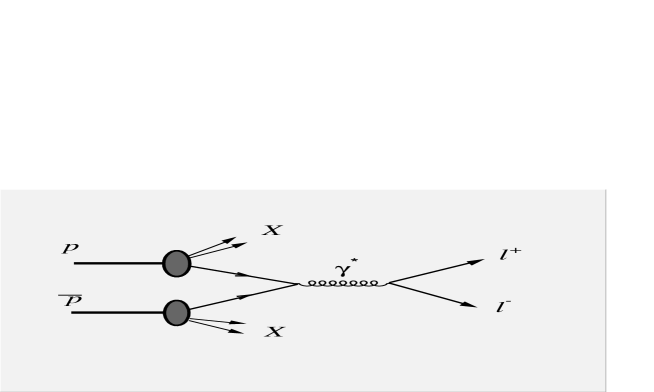
Figure 1: $\bar{p}p\rightarrow l^{+}l^{-}+X$ process

For this aim we utilized here, as for the first step, the well known event generator PYTHIA [15], which is based on the ideas of the quark parton model and is well tested and widely used for the simulation of hadron-hadron interactions. PYTHIA simulation is based on the use of the amplitudes of the relativistic quantum field theory. This allows a proper account of the relativistic kinematics during simulation of different physical variables distributions specific for $\mu^{+}\mu^{-}$- or $e^{+}e^{-}$- pair produced in event. In our case we use the perturbative QCD/QED parton level amplitude of the lepton pair production process ${q\bar{q}\to\gamma^{*}\to l^{+}l^{-}}$ with the continuous spectrum of the invariant mass of lepton pair and the amplitude of J/$\Psi$ - resonance production process $p+\bar{p}\to J/\Psi+X\to l^{+}l^{-}+X$, where J/$\Psi$ decays through the leptonic channel ($J/\Psi\to l^{+}l^{-}$, $l=\mu,e$ ), which are implemented into the PYTHIA package.

Let us underline that the results obtained here on the basis of PYTHIA simulation in some sense may allow to fix the predictions for lepton kinematical distributions which may be obtained in the framework of perturbative theory approach. Therefore, they may be useful at the analysis stage for defining the boundary between the predictions of perturbative and nonperturbative theoretical approaches.

In Section 2 we present the kinematical distributions for individual leptons. The set of plots with energy, transverse momentum and angle distributions are given together with some plots which show different kinds of Energy-Energy, Energy-Angle and Angle-Angle correlations between the physical variables of the leptons produced via the leading order quark level subprocess $q\bar{q}\rightarrow l^{+}l^{-}$. The estimations of events loss due to a possible different choice of geometrical parameters of muon system and electromagnetic calorimeter are given.

Section 3 is devoted to another channel of lepton pair production. The process of $J/\Psi$ resonance production (with its decay into a lepton pair) $p+\bar{p}\to J/\Psi+X\to l^{+}l^{-}+X$ ($l=\mu,e$) is simulated by use of PYTHIA6.4 which includes a sizeable set of parton level subprocesses that can give a contribution to this process. This process was chosen to be a benchmark process for PANDA experiment (see TPR [6]). Thus, the obtained here kinematical distributions of the final state leptons shall have a practical application. In the following we shall call this process as resonance production to distinguish it from the process considered in Section 2, where the invariant mass of two leptons produced in quark level subprocess $q\bar{q}\rightarrow l^{+}l^{-}$ has a continuum spectrum.

Section 4 includes the distributions of the invariant mass and some other physical variables which are characteristic for the signal lepton pair as a whole system. The most interesting among them is the total transverse momentum of a lepton pair which is connected with the intrinsic transverse velocity of a quark inside the proton.

In Section 5 we estimate the size of the kinematical region in $x-Q^{2}$ plane which can be available for measuring the quark distributions in PANDA experiment.

The problems connected with the background from the fake leptons, which may appear together with the signal lepton pair in one and the same event due to meson decays, as well as with the background from other than $q\bar{q}\rightarrow l^{+}l^{-}$ subprocesses, are discussed in Sections 6 and 7, correspondingly. Also we present a set of cuts which allows to separate the background events from the signal ones. The efficiencies of the proposed cuts are also given.

In Section 8 we outline some important physical measurements which can be done by studying the lepton pair production at the energies available for PANDA experiment.

It is worth mentioning that the results presented here can also be useful for the future physical analysis of hadron decays at PANDA because the contribution from $q\bar{q}\rightarrow l^{+}l^{-}$ events may be one of the main background sources in this kind of a study.

2 Distributions of leptons produced in $p\bar{p}$ collisions

We use PYTHIA6 to generate two samples (separately for muons and electrons) of 100 000 ”$\bar{p}p\rightarrow l^{+}l^{-}+X$” events which include the $2\rightarrow 2$ quark level ${q\bar{q}\to\gamma^{*}\to l^{+}l^{-}}$ subprocess. In the following, these events will be called as ”signal events”, and the muons/electrons produced in this subprocess will be called as ”signal” leptons. The fake leptons which are produced in hadron (mainly mesons) decays in the same signal event will be called ”decay” leptons. The simulation is done starting from the assumption of the ideal muon system and electromagnetic calorimeter covering $360^{o}$. No any cuts are used in the following Sections. They will be discussed in the subsection 6.5 and the Section 8.

We consider the case where both initial-state radiation (ISR) and final-state radiation (FSR) are switched on simultaneously by choosing the corresponding values of PYTHIA parameters. Also we have used the CTEQ3L parametrization of parton distributions and the default value of the parameter, which allows one to take into account the primordial $k_{T}$-effect (the effect of quark Fermi motion inside the hadron).

First we consider the distributions of some physical variables which describe the kinematics of individual leptons belonging to the $l^{+}l^{-}$ pair. Simulation shows that there is no difference between $e^{+}e^{-}$ and $\mu^{+}\mu^{-}$ distributions. In all the following figures the vertical axis shows the number of events (per bin) that may be expected per year ($10^{7}sec$) for the luminosity $L=2\cdot 10^{32}cm^{-2}s^{-1}$ (=2 $\cdot 10^{5}mb^{-1}s^{-1}$). The total number of expected events per year are shown as ”Integral” values in the figures. Let us underline that this number can be treated only as an estimation because it strongly depends on the models used in PYTHIA which is basically designed for much higher energies.

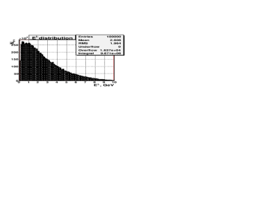
a) b)

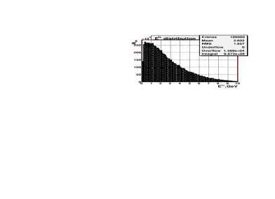
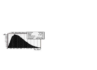
c) d)

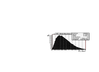
e) f)

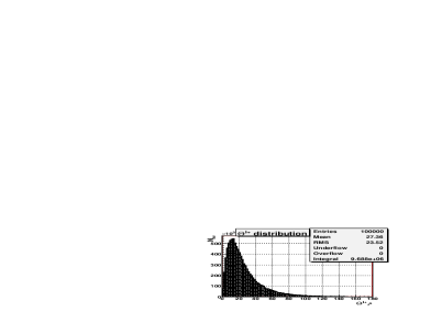
Figure 2: Distributions of number of signal leptons versus: the energy $E^{l^{(+/-)}}$ (top row, plots a and b), the modulus of transverse momentum $P_{T}^{l^{(+/-)}}$ (middle row, plots c and d) and the polar angle $\theta^{l^{(+/-)}}$ (bottom row, plots e and f). Left column: $l^{-}$, right column $l^{+}$.

The distributions of the number of generated signal events ($N_{ev}$) versus the the energy $E^{l^{(+/-)}}$ of the signal leptons, as well as versus the modulus of the transverse momentum $P_{T}^{l^{(+/-)}}$ and of the polar (zenith) angles $\theta^{l^{(+/-)}}$, measured from the z-axis directed along the beam line, are given (top to bottom) in Fig.2. The left column of Fig.2 is for $l^{-}$ distributions and the right one is for $l^{+}$. One can see from the top row of Fig.2 (plots a and b) that the most part of leptons energy is contained in the interval $0<E^{l}<10$ GeV. Its spectrum has a mean value $<E^{l}>=2.6$ GeV and a peak at $E^{l}_{peak}\approx 0.5$ GeV. The $P_{T}^{l}$ spectrum (see the middle row plots c and d of Fig.2) has an analogous peak at $P^{l}_{T_{peak}}\approx 0.4$ GeV. Behind their peaks both $E^{l}$ and $P_{T}^{l}$ spectra fall rather steeply. The main part of $P_{T}^{l}$ spectrum is confined within a rather narrow interval $0<P_{T}^{l}<2$ GeV.

The number of events spectrum versus the polar angle ${\theta^{l}}$ (see bottom row plots e and f of Fig.2) has a peak around ${\theta^{l}}\approx 10^{o}$ and the mean value $<\theta^{l}>=27.3^{o}$. One sees that while the most of signal leptons fly in the forward direction ($\theta^{l}<90^{o}$) there is still a small number of them which fly into the back hemisphere ($\theta^{l}>90^{o}$).

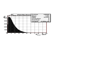
a) b)

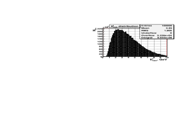
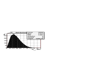
c) d)

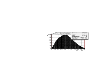
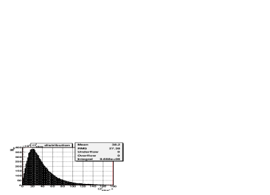
e) f)

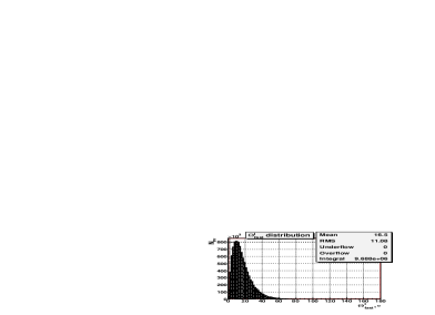
Figure 3: Distributions of number of signal leptons versus: the energy $E^{l^{(+/-)}}$ (top row, plots a and b), the modulus of the transverse momentum $P_{T}^{l^{(+/-)}}$ (middle row, plots c and d) and the polar angle $\theta^{l^{(+/-)}}$ (bottom row, plots e and f) . Left column: low energy ”slow” leptons, right column: high energy ”fast” leptons.

Fig.3 includes the set of plots done separately for the signal leptons having the largest energy $E^{l}_{fast}$ (right column) in the lepton pair and for the leptons having a smaller energy $E^{l}_{slow}$ in the pair (left column). We shall call them, correspondingly, as ”fast” and ”slow” leptons. One can see that the energy spectrum of fast signal leptons (plot b) increases rather fast from the point $E^{l}_{fast}\approx 0.5$ GeV (more than $90\%$ of fast leptons have $E^{l}_{fast}>1$ GeV) up to the peak position at the point $E^{l}_{fast}\approx 2.5$ GeV ($<E^{l}_{fast}>$ = 3.85 GeV). Then it smoothly vanishes at $E^{l}_{fast}=10$ GeV.

In contrast to this picture, the analogous spectrum of the less energetic signal leptons (plot a) starts sharply from zero and reaches a peak at $E^{l}_{slow}\approx 0.4$ GeV (where the spectrum of the fast leptons only starts). Then it goes down and practically vanishes at the point $E^{l}_{slow}\approx 5$ GeV. One may see that the energy spectrum of slow leptons plot a in a pair is more than by half shorter than that one of fast leptons plot b and the mean value of slow leptons energy $<E^{l}_{slow}>=1.36$ GeV is about 3 times less than the mean energy of fast leptons $<E^{l}_{fast}>=3.85$ GeV.

The difference between the $PT^{l}$ spectra of fast and slow leptons is not so large (see, correspondingly, plots d and c in the middle row of Fig.3). They differ only by about 400 MeV shift to the left of the peak position of the slow leptons spectrum and about 340 MeV analogous shift of their mean transverse momentum value. Both of these spectra demonstrate that the main part of slow and fast leptons has $PT^{l}>0.2$ GeV.

The bottom row of the plots demonstrates that the polar (zenith) angle spectrum of less energetic leptons ${\theta^{l}_{slow}}$ (Fig.3 e) is shifted to the higher values as compared to the spectrum of fast leptons ${\theta^{l}_{fast}}$ (Fig.3 f). Its mean value $<{\theta^{l}_{slow}}>=38.2^{o}$ is more than twice as large as the analogous mean value of fast leptons: $<{\theta^{l}_{fast}}>=16.5^{o}$. Thus, we can conclude that almost all fast leptons fly in the forward direction (${\theta^{l}_{fast}}<80^{o}$) and their spectrum practically finishes at ${\theta^{l}_{fast}}\approx 60^{o}$ (plot f) while about $17\%$ of slow leptons (plot e) have ${\theta^{l}_{slow}}>60^{o}$. It is worth noting that about $5\%$ of slow leptons may scatter into the back hemisphere.

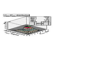
a) b)

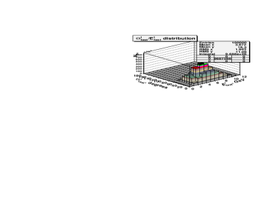
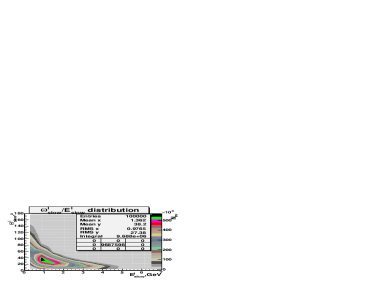
c) d)

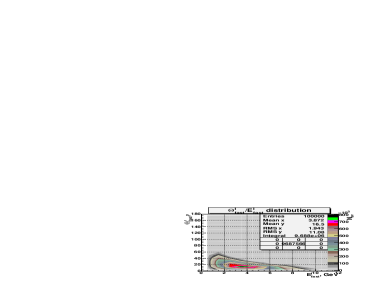
Figure 4: Angle-Energy correlations. a) and c): ${\theta^{l}_{slow}}/{E^{l}_{slow}}$ correlation for slow leptons, b) and d): ${\theta^{l}_{fast}}/{E^{l}_{fast}}$ correlation for fast leptons. Plots c) and d) are the pojections of 3D plots a) and b) on ${\theta^{l}}-{E^{l}}$ planes.

Fig.4 contains two 3-Dimensional ”Angle-Energy” correlation plots for slow ${\theta^{l}_{slow}}/{E^{l}_{slow}}$ (plot $\bf{a}$) and fast ${\theta^{l}_{fast}}/{E^{l}_{fast}}$ (plot $\bf{b}$) leptons in signal pairs. Their vertical axes show the distribution of number of signal events ($N_{ev}$) multiplied by $10^{3}$. 2-dimensional plots $\bf{c}$ and $\bf{d}$ are obtained by projection of plots $\bf{a}$ and $\bf{b}$ onto the $\theta-E$ planes. This allows to show the boundary contours of regions with different density of number of events. The right-hand color vertical strip in each plot $\bf{c}$ and $\bf{d}$ shows the correspondence between the contour color and the density of events. This color strip plays the role of the vertical z axis with the number of events $N_{ev}$ shown in plots a and b. Plots c and d of Fig.4 show the kinematical regions in $\theta-E$ plane which are covered by slow and fast leptons, respectively. Plot c of Fig.4 demonstrates that the value of the polar angle of slow leptons ${\theta^{l}_{slow}}$ drops much steeply with the growth of their energy as compared to the behavior of the polar angle of fast lepton ${\theta^{l}_{fast}}$ shown at the plot $\bf{d}$.

After discussion of individual lepton distributions let us turn to the distributions that characterize the produced pair of leptons as a whole system. Fig.5 shows the Energy-Energy $E^{l}_{slow}/E^{l}_{fast}$ (plots a and c) and Angle-Angle ${\theta^{l}_{slow}}/{\theta^{l}_{fast}}$ (plots b and d) correlations. Plots c and d are the projections of 3D plots a and b on $E^{l}_{slow}-E^{l}_{fast}$ and ${\theta^{slow}}-{\theta^{fast}}$ planes, correspondingly.

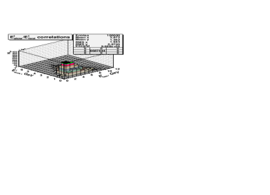
a) b)

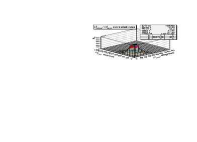
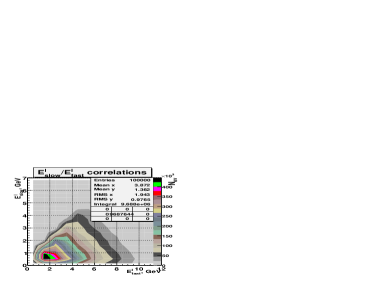
c) d)

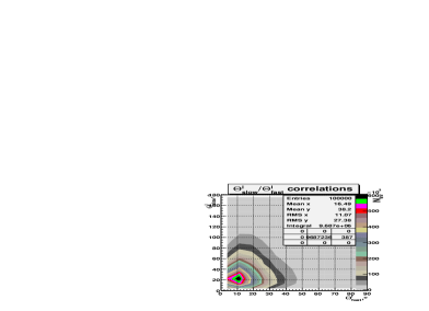
Figure 5: a) and c): Energy-Energy $E^{l}_{slow}/E^{l}_{fast}$ correlations. b) and d): Angle-Angle $\theta^{l}_{slow}/\theta^{l}_{fast}$ correlations. Plots c) and d) are the projections of 3D plots a) and b) on $E^{l}_{slow}-E^{l}_{fast}$ and ${\theta^{slow}}-{\theta^{fast}}$ planes correspondingly.

Data taking of searched signal events is strongly influenced by the cuts on lepton energies which can be imposed from below to suppress the electronic noise and some other background which can be provided by detector effects. The analysis of the plots a and c of Fig.5 is summarized in the Table 1. It demonstrates (in $\%$) the loss of signal events due to application of the kinematical cut $E_{fast}^{l},E_{slow}^{l}\geq E_{cut}$ which sets the lower limit $E_{cut}$ on the value of lepton energy.

Table 1: Efficiency of the $E_{fast}^{l},E_{slow}^{l}\geq E_{cut}$ cut

$E_{cut}$ ( in GeV)	The loss of signal events ( in $\%$)
0.5	24
1.0	45

The efficiency of collection of signal events which contain leptonic $l^{+}l^{-}$ pairs also depends on the angle coverage by the muon system and the Electromagnetic Calorimeter (ECAL). Plots $\bf{b}$ and $\bf{d}$ of Fig.5 show the Angle-Angle ${\theta^{l}_{slow}}/{\theta^{l}_{fast}}$ lepton correlation. The results of its analysis are given in the Table 2 which demonstrates which part (in $\%$) of signal events would be lost due to imposing the upper limit $\theta_{cut}$ (i.e. ${\theta^{l}_{slow}},{\theta^{l}_{fast}}\leq\theta_{cut}$ cut) on the size of muon system or ECAL.

Table 2: Efficiency of the ${\theta^{l}_{slow}},{\theta^{l}_{fast}}\leq\theta_{cut}$ cut

$\theta_{cut}^{0}$  ( in 0)	The loss of signal events ( in $\%$ )
20	80
40	39
60	17
90	5

The last line of Table 2 shows that even in the case when the muon system or the ECAL would cover the angle region $\theta^{l}\leq 90^{o}$, about $5\%$ of the events containing the $l^{+}l^{-}$ signal pairs would be lost. Nevertheless, such geometrical boundary allows to keep about 95$\%$ of signal events with electron or muon pairs. Therefore, we consider this choise of polar angle upper limit as a preferable one for the study of MMTDY process of lepton pair production (with the continuous mass spectrum of this pair).

3 Leptons from J/$\Psi$ decay

The process of J/$\Psi$ resonance production with its further decay into a lepton ($l=\mu,e$) pair $p+\bar{p}\to J/\Psi+X\to l^{+}l^{-}+X$ (see one of the possible reaction on Fig.6) was considered in the PANDA TDR [6] as one of the benchmark processes. Therefore, modeling of the kinematical (energy, transverse momentum and angle) distributions of final state leptons is of practical interest.

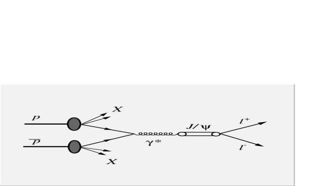
Figure 6: $\bar{p}p\rightarrow J/\Psi+X\to l^{+}l^{-}+X$ process

Like in previous Section, we use the same event generator PYTHIA6.4 which includes the following set of subprocesses with J/$\Psi$ production:

1) $q_{i}\bar{q}_{i}\to\gamma^{*}\to c\bar{c}\to J/\Psi\to l^{+}l^{-}+X$                  86) $gg\to J/\Psi+g\to l^{+}l^{-}+X$ [10]
106) $gg\to J/\Psi+\gamma\to l^{+}l^{-}+X$ [11]                       421) $gg\to c\bar{c}[^{3}S_{1}^{(1)}]g\to l^{+}l^{-}+X$ [12]
422) $gg\to c\bar{c}[^{3}S_{1}^{(8)}]g\to l^{+}l^{-}+X$ [12]                      423) $gg\to c\bar{c}[^{3}S_{0}^{(8)}]g\to l^{+}l^{-}+X$ [12]
424) $gg\to c\bar{c}[^{3}P_{J}^{(8)}]g\to l^{+}l^{-}+X$ [12]                      425) $gq\to c\bar{c}[^{3}S_{1}^{(8)}]q\to l^{+}l^{-}+X$ [12]
426) $gq\to c\bar{c}[^{3}P_{J}^{(8)}]q\to l^{+}l^{-}+X$ [12]                      427) $gg\to c\bar{c}[^{3}S_{1}^{(1)}]q\to l^{+}l^{-}+X$ [12]
428) $q\bar{q}\to c\bar{c}[^{3}S_{1}^{(8)}]g\to l^{+}l^{-}+X$ [12]                      429) $q\bar{q}\to c\bar{c}[^{1}S_{0}^{(8)}]g\to l^{+}l^{-}+X$ [12]
430) $q\bar{q}\to c\bar{c}[^{3}P_{J}^{(8)}]g\to l^{+}l^{-}+X$ [12]                    431) $gg\to c\bar{c}[^{3}P_{0}^{(1)}]g\to l^{+}l^{-}+X$ [12]
432) $gg\to c\bar{c}[^{3}P_{1}^{(1)}]g\to l^{+}l^{-}+X$ [12]                     433) $gg\to c\bar{c}[^{3}P_{2}^{(1)}]g\to l^{+}l^{-}+X$ [12]
434) $gq\to c\bar{c}[^{3}P_{0}^{(1)}]q\to l^{+}l^{-}+X$ [12]                      435) $gq\to c\bar{c}[^{3}P_{1}^{(1)}]q\to l^{+}l^{-}+X$ [12]
436) $gq\to c\bar{c}[^{3}P_{2}^{(1)}]q\to l^{+}l^{-}+X$ [12]                      437) $qq\to c\bar{c}[^{3}P_{0}^{(1)}]g\to l^{+}l^{-}+X$ [12]
438) $q\bar{q}\to c\bar{c}[^{3}P_{1}^{(1)}]g\to l^{+}l^{-}+X$ [12]                      439) $q\bar{q}\to c\bar{c}[^{3}P_{2}^{(1)}]g\to l^{+}l^{-}+X$ [12]

The main contribution to the total cross section of J/$\Psi$ production comes from the following three subprocesses:
1)    $q_{i}\bar{q}_{i}\to\gamma^{*}\to c\bar{c}\to J/\Psi\to l^{+}l^{-}+X$
428) $q\bar{q}\to c\bar{c}[^{3}S_{1}^{(8)}]g\to l^{+}l^{-}+X$
430) $q\bar{q}\to c\bar{c}[^{3}P_{J}^{(8)}]g\to l^{+}l^{-}+X$

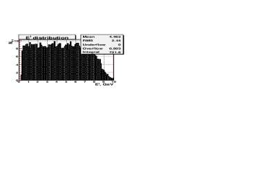
a) b)

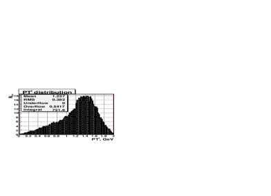
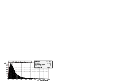
c) d)

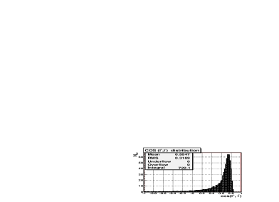
Figure 7: Distributions of the leptons from $J/\Psi$ decay into $l^{+}l^{-}+X$: a) energy $E^{l^{(+/-)}}$, b) modulus of the transverse momentum $P_{T}^{l^{(+/-)}}$; c) polar angle $\theta^{l^{(+/-)}}$; d) cos of the opening angle between the leptons in $l^{+}l^{-}$ pair.

Distributions of the final state leptons, produced in J$/\Psi$ decay, are shown in Fig.7. They are obtained without a use of any cuts and cover the same ranges as the leptons produced in the continuum case (see Fig.2). From comparison of these two Figures one can see that the energy and momentum distributions presented in Fig.7 look very different to those of Fig.2. Thus, plot a of Fig.7 shows a rather flat distribution of the number of events versus the energy of leptons from J$/\Psi$ decay, while the analogous plots a and b of Fig.2 demonstrate that the most part of leptons produced in the continuum case have small energies $E^{l}<1$ GeV. Analogously, as seen from the plot b of Fig.7, the peak of $P_{T}^{l}$ distribution in a case of J$/\Psi$ production appears at the point $P_{T}^{l}\approx 1.4$ which is more than three times higher than the maximum value of $P_{T}^{l}$ in the plot b of Fig.2 ($\approx 0.4$ GeV). As one can see from the plot d of Fig.7, the maximum of cos $(l^{+},l^{-})$ is at $\approx$ 0.75. This value corresponds to the opening angle between the leptons of $\approx 42^{o}$.

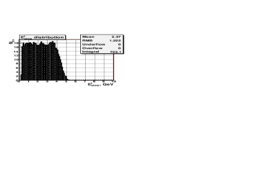
a) b)

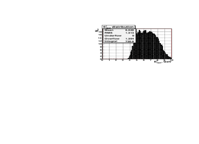
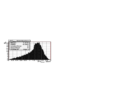
c) d)

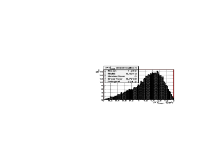
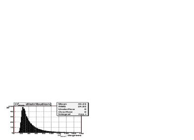
e) f)

Figure 8: Distributions of the leptons from $J/\Psi$ decay into $l^{+}l^{-}+X$: energy $E^{l^{(+/-)}}$ (top row), modulus of the transverse momentum $P_{T}^{l^{(+/-)}}$ (middle row) and polar angle $\theta^{l^{(+/-)}}$ (bottom row). Left column: low energy ”slow” leptons, right column: high energy ”fast” leptons.

Fig.8 is the analog of Fig.3. It presents the distributions of the same leptons produced in J$/\Psi$ decay, but separately for ”slow” and ”fast” ones. One can see that the plots a and b of Fig.8 look much more different from the plots a and b of Fig.3. The main difference is that the energy spectra of slow ($E_{slow}$) and fast ($E_{fast}$) leptons, shown in the plots a and b of Fig.8, cover very different energy intervals which have very small area of their overlapping in the region of $E^{l}\approx 4-5$ GeV. It is also seen from the plots c and d of Fig.8 that transverse momenta of both slow and fast leptons have a rather close mean values about $P_{T}^{l}\approx 1.4$. Plots e and f of Fig.8 demonstrate a good separation of polar angle distributions of slow and fast leptons. It is seen that the most part of the spectrum of slow leptons lay behind the 20^o, while the spectrum of fast leptons polar angles ranges in the interval from 0^o to 25^o and has the mean value $\theta_{fast}^{l}=$12.12 GeV.

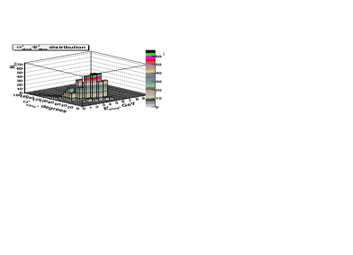
a) b)

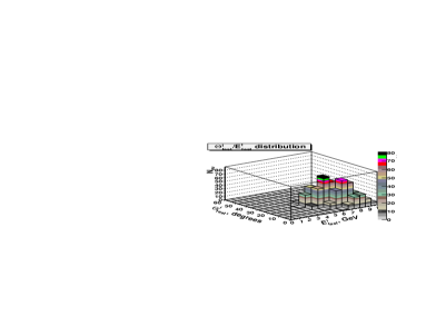
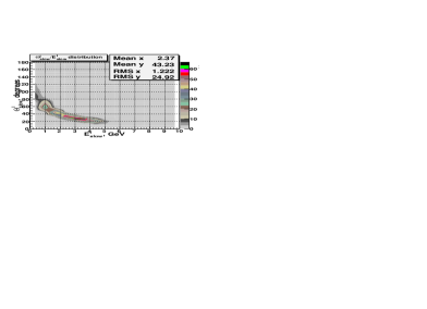
c) d)

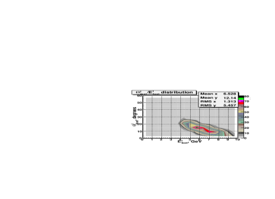
Figure 9: Angle-Energy correlations. a) and c): ${\theta^{l}_{slow}}/{E^{l}_{slow}}$ correlation for slow leptons, b) and d): ${\theta^{l}_{fast}}/{E^{l}_{fast}}$ correlation for fast leptons. Plots c) and d) are the projections of 3D plots a) and b) onto ${\theta^{l}}/{E^{l}}$ plane.

Fig.9 includes the plots which show Angle-Energy correlations of the leptons produced in $J/\Psi$ decay. Plots a and c are for slow leptons, plots b and d are for fast leptons. They are also very different from those shown in Fig.4 for the case of continuum lepton pair production via the process $p\bar{p}+p\to\gamma^{*}\to l^{+}l^{-}+X$. It is seen that fast and slow leptons produced in $J/\Psi$ decay cover very different and well separated regions (see plots c and d of Fig.9) while in the continuum case (see plots c and d of Fig.4) the distributions of fast and slow leptons have a wide area of their overlapping. These regions are rather narrow and have a strip form, that looks different from the case of continuum lepton pair production (see plots c and d of Fig.4).

It is of interest to compare the Energy-Energy and Angle-Angle correlation plots which are presented in Fig.10 for the case of lepton pair production from $J/\Psi$ resonance decay and those shown in Fig.5 for leptons production in continuum case. It is seen from the plot c of Fig.10 that the energy region covered in $E_{slow}-E_{fast}$-plane in the case of $J/\Psi$-resonance production process fits well into the right corner of the region covered covered in the $E_{slow}-E_{fast}$-plane shown in the plot c of Fig.5 for the case of continuum mass MMTDY process of lepton-antilepton pair production.

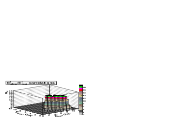
a) b)

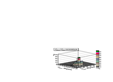
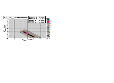
c) d)

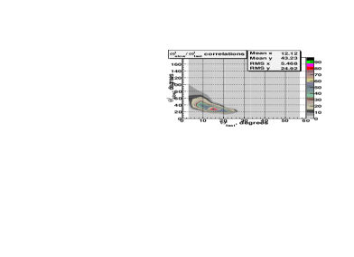
Figure 10: a) and c): Energy-Energy $E^{l}_{slow}/E^{l}_{fast}$ correlations, b) and d): Angle-Angle $\theta^{l}_{slow}/\theta^{l}_{fast}$ correlations. Plots c) and d) are the pojections of 3D plots a) and b) onto $E^{l}_{slow}/E^{l}_{fast}$ and ${\theta^{slow}}-{\theta^{fast}}$ plane correspondingly.

Moreovere, the analogous comparison of the plot d of Fig.10 with the plot d of Fig.5 allows to make an important observation that the area covered in the $\theta_{slow}-\theta_{fast}$ plane fits well into the analogous aria of Angle-Angle correlation plot in Fig.5. From here one can conclude that the choice of polar angle boundary for muon system geometry, which was proposed in Section 2 basing on the analysis of MMTDY process, would be quite suitable for the study of both benchmark $J/\psi$ and MMTDY channels of lepton-antilepton pair production.

4 Distributions of the invariant mass, energy
and transverse momenta of lepton pairs

We consider here a set of physical variables which characterize a produced lepton pair as a whole system. These variables are constructed from the components of the total 4-momentum of initial state quark-antiquark system $P^{q\bar{q}}_{\alpha}=P^{q}_{\alpha}+P^{\bar{q}}_{\alpha}$, ($\alpha=0,1,2,3$) and its analog ${P^{l^{+}l^{-}}_{\alpha}=P^{l^{+}}_{\alpha}+P^{l^{-}}_{\alpha}}$ for a lepton pair ($P^{l^{\pm}}$ is the 4-momentum of lepton l) . Figs.11a, 11b show, correspondingly, the distributions of the invariant masses of initial-state quark-antiquark pair

$$M_{inv}^{q\bar{q}}=\sqrt{(}P^{q\bar{q}})^{2},$$ (1)

and the invariant mass of the final-state lepton-antilepton pair

$$M_{inv}^{l^{+}l^{-}}=\sqrt{(}P^{l^{+}l^{-}})^{2}=Q,~{}~{}~{}{Q^{2}=q^{2}=(P^{l^{+}}_{\alpha}+P^{l^{-}}_{\alpha})^{2}},$$ (2)

been produced in the signal process $\bar{p}p\rightarrow l^{+}l^{-}+X$ which goes through the quark level subprocess ${q\bar{q}\to\gamma^{*}\to l^{+}l^{-}}$. Both invariant mass distributions look rather similar. They are rather short and drop steeply with the growth of invariant mass. The distribution of the invariant mass $M_{inv}^{q\bar{q}}$ of the initial-state $q\bar{q}$-system sharply starts at the point $M_{inv}^{q\bar{q}}=1$ GeV which is the left boundary point due to the internal PYTHIA restriction on the lowest value of the invariant mass of the initial state two-body system of any fundamental quark-parton $2\to 2$ subprocess. The spectrum finishes at $M^{q\bar{q}}_{inv}=M^{l^{+}l^{-}}_{inv}\approx 2.5$ GeV.

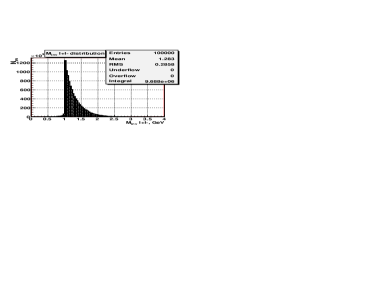
a) b)

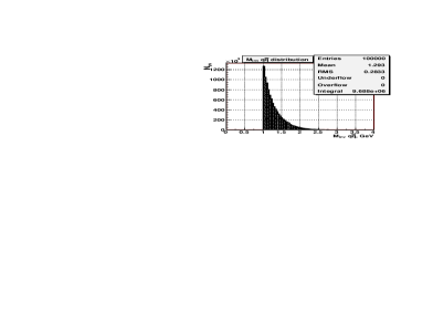
Figure 11: Distribution of number of signal events versus the invariant mass. a) The invariant mass of initial-state quark-antiquark system $M_{inv}^{q\bar{q}}$; b) The invariant mass of final-state lepton-antilepton pair $M^{l^{+}l^{-}}_{inv}$.

Different to the spectrum of the invariant mass of the initial-state $q\bar{q}$-system, the invariant mass $M_{inv}^{l^{+}l^{-}}$ of the final-state $l^{+}l^{-}$ system has a very small tail at smaller than 1 GeV values $M^{l^{+}l^{-}}_{inv}<1$ GeV (see Fig.11a) .

The spectrum of the total lepton pair energy ${E^{l^{+}l^{-}}=E^{l^{+}}+E^{l^{-}}}$ is shown in Fig.12a. It is seen that the lepton pair total energy distribution is by about 2 GeV longer than the spectrum of the fast leptons energy $E^{l}_{fast}$ (see Fig.3b).

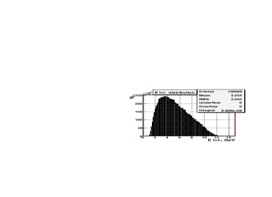
a) b)

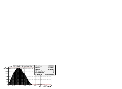
Figure 12: Distribution of number of signal events versus: a) the total lepton pair energy ${E^{l^{+}l^{-}}}$; b) the total transverse momentum $P^{l^{+}l^{-}}_{T}$ of the lepton pair.

The mean value of the total energy of the lepton pair, as seen from Fig.12${\bf{a}}$, is about 5 GeV. From the same plot of Fig.12 it is clearly seen that in more than a half of events the lepton pair energy lays in the interval $4\leq{E^{l^{+}l^{-}}}\leq 12$ GeV. So, one can conclude that the produced lepton pairs are rather energetic and they can carry away quite a noticeable part of the total energy of the colliding $\bar{p}p$-system.

The distribution of the longitudinal component ${P^{l^{+}l^{-}}_{z}=P^{l^{+}}_{z}+P^{l^{-}}_{z}}$ of the total 4-momentum of lepton pair system (not shown here) has a shape which is very similar to the energy ${E^{l^{+}l^{-}}}$ spectrum. The explanation of this fact follows from the shape of the distribution of the modulus of lepton pairs total transverse momentum

$$P^{l^{+}l^{-}}_{T}=|\vec{P}^{l^{+}l^{-}}_{T}|=|\vec{P}^{l^{+}}_{T}+\vec{P}^{l^{-}}_{T}|,$$ (3)

which is presented as the “$P_{T}^{l^{+}l^{-}}$ distribution” in Fig.12b. One may see that the distribution of the transverse component $P^{l^{+}l^{-}}_{T}$ is much more narrow than that one of the energy ${E^{l^{+}l^{-}}}$. It covers the region $0<P^{l^{+}l^{-}}_{T}<2$ GeV, like it was in a case of a single lepton distribution (see plots c and d of Fig.2). $P^{l^{+}l^{-}}_{T}$ has a peak position at about 1 GeV, that is twice as large as the analogous peak position of a single lepton $P^{l}_{T}$ shown in the same plots c and d of Fig.2. Thus, we see that the main contribution to the value of lepton pair energy comes from the longitudinal component ${P^{l^{+}l^{-}}_{z}}$.

It is worth noting that according to Fig.1 the square of the invariant mass $(M_{inv}^{l^{+}l^{-}})^{2}=Q^{2}=q^{2}=(P^{l^{+}}+P^{l^{-}})^{2}$ has the meaning of the square of the momentum transferred from the quark-antiquark pair to the lepton pair. Therefore, it plays the same role as the $Q^{2}$ in the processes of deep-inelastic scattering (DIS) of lepton over the proton. From this point of view the diagram shown in Fig.1 looks like the cross chanel analog of the diagram of DIS scattering of a lepton over the proton with the inclusive production of a proton in the final state. The essential difference is that in DIS case the momentum transferred is defined by the relation $q_{dis}=P^{l}_{in}-P^{l}_{out}$ ($P^{l}_{in}$ and $P^{l}_{out}$ are, respectively, the 4-momenta of incoming and outgoing leptons) , which differs from the definition of $Q^{2}$ given above for the case of MMTDY process. Therefore, its square has the negative value $q_{dis}^{2}\leq$ 0, while in MMTDY process its square is positive: $q^{2}\equiv(P^{l^{+}}+P^{l^{-}})^{2}\geq 0$.

To conclude this Section let us mention that the measurement of the invariant mass of lepton pair would allow to separate the background to $J/\psi$ production events up to a good accuracy.

5 Estimation of the size of $x-Q^{2}$ region available for measurement of proton structure function

The distributions of Bjorken x-variables are shown in Fig.13 for up- (plot a) and down- (plot b) quarks . They represent the corresponding quark components of the proton structure function which was used in the present simulation with CTEQ3L PDF.

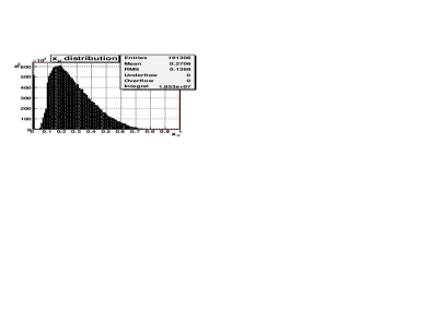
a) b)

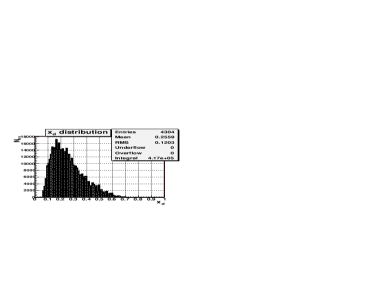
Figure 13: x distributions of valence: a) up quarks; b) down quarks.

The most ineresting for us is the information about the size of the x-region which will be available at PANDA energies. We see from both plots of Fig.13 that x-varaiable spans the interval $0.05<x<0.7$. Recall that in $\bar{p}p$ collisions the transverse momentum $P_{T}$ plays the role of the transferred momentum q.

So, combining the results from Figs.11 and 13 we can conclude that, according to the results of simulation with PYTHIA, we can hope to get the information about valence quark distributions in the kinematical region defined by the following boundaries: $0.05\leq x\leq 0.7$ and $Q^{2}\leq 6.2$ GeV ($Q^{2}\equiv q^{2}=(P^{l^{+}l^{-}}_{T})^{2}$). The important point that should be stressed here is that different to lepton-hadron scattering, which provides the information about the structure functions in the region of negative, i.e. ”space-like” values of the square of transversed momentum $q_{dis}^{2}=(P^{l}_{in}-P^{l}_{out})^{2}$, the ”annihilation” process $\bar{p}p\rightarrow l^{+}l^{-}+X$ allows to get the information about the structure functions in a region of positive, i.e. ”time-like” values of $q^{2}\geq 0$. Such a measurement of quark distributions will be a good supplement to the planned measurement of proton elastic formfactor in the region of ”time-like” values of $q^{2}\geq 0$ (see [6]) and the planned measurements of deep-inelastic process in a region of small values of $q^{2}\leq 0$ at JLab and DESY.

6 Fake leptons in signal events

The signal events, defined by the $q\bar{q}\rightarrow l^{+}l^{-}$ subprocess, also contain some hadrons in the final state. Fortunately, their number is essentialy restricted by the upper limit on the beam energy that may be available at PANDA experiment. This circumstance may simplify greatly the identification of final state particles and the physical analysis due to reduction of the phase space and therefore to the reduction of the number of hadrons and other particles which may be produced in event directly or in the decays cascades of other hadrons. These hadrons may decay within the detector volume and thus produce the background leptons which may fake the signal leptons ($\mu$, e) produced in a signal annihilation subprocess. In signal events with electron-positron pair producton the fake electrons/positrons may appear also from muon decays.

In this Section we shall consider separatly the signal events with muon pair production (subsections 6.1 and 6.3) and the signal events with electron pair production (subsection 6.4). The subsection 6.2 includes the discussion of different kinematical distributions for charged pions which povide the main contribution to fake muons. Our analysis of fake leptons is based on two different samples. One of them is the sample with signal muon pair events production while the second one with electron pair production events. This samples were used in Section 2.

6.1 Fake muons

We shall first discuss the case of background muons which may be produced additionally to a signal ”$\mu^{+}\mu^{-}$”- pair in the signal events due to hadron decays. For this reason, we shall call these fake muons also as “decay muons” (in the following we do not distinguish $\mu^{+}$ and $\mu^{-}$). The distribution which shows the number of the main hadronic “parents” of muons in signal events is presented in the plot a of Fig.14, while Fig.14 b shows the distribution of muon “grandparents”, i.e. the “parents of muon parents”.

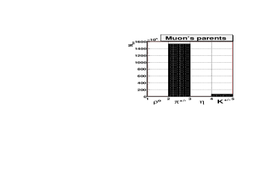
a) b)

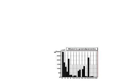
Figure 14: Distributions of: a) parents of fake $\mu$’s; b) grandparents of fake $\mu$’s

The correspondence between the bin number on the x-axis and the name of the related grandparent of the muon can be found from the right column of Table 7 of the Section 11 (Appendix: Tables). ) is of about one order less. From Fig.14 b and the right column of Table 7 of the Section 11 (Appendix: Tables) one can conclude that the strings (bin 2 in Fig.14 b), $\omega$ (bin 6) and $\Lambda^{0}$ (bin 20) are the main grandparents of muons. It is of interest to consider in more detail the kinematical distributions of charged pions as the main source of fake muons and to compare them with the distributions of produced muons. We shall do it in the following subsection.

6.2 Kinematical distributions of parent pions

The left-hand side of Figure 15 includes (like Figs.2 and 3) three plots (a, c, e) containing the distributions (top to bottom) of the number of events versus the energy $E_{\pi}$ (plot a), the transverse momentum ${PT_{\pi}}$ (plot c) and the polar angle $\theta_{\pi}$ (plot e) of charged pions which appear in the sample of generated by PYTHIA signal muon events (100 000) based on the quark level subprocess $q+\bar{q}\to\mu^{+}\mu^{-}$ (this sample was discussed in the Section 2 and in the begining of this Section).

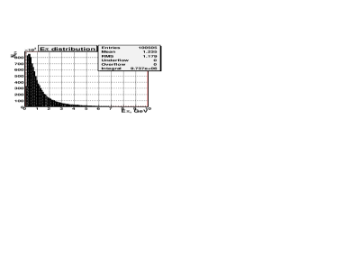
a) b)

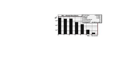
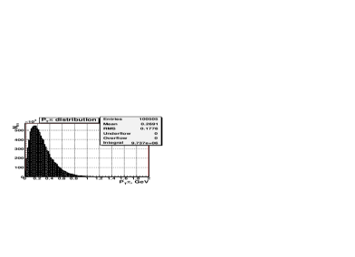
c) d)

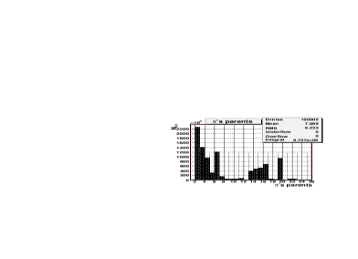
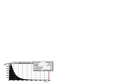
e) f)

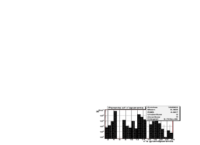
Figure 15: Left column: distributions of the number of pions versus a): the energy $E_{\pi}$; c): transverse momentum $P_{T}{\pi}$ and e): polar angle ${\theta_{\pi}}$ of the produced pions. Right column: distributions b): of the total number $N_{\pi}$ of charged ${\pi}$-mesons in the signal events; d): of the particles that give birth to the pions ($\pi$’s parents) and f): of the particles which are parents to $\pi$’s parents

The plot b in the same Fig.15 shows the distribution of number $N_{\pi}$ of charged ${\pi}$-mesons produced per event in generated signal events. The first left bin in this plot shows the number of events without charged pions. One may see that there is a huge number of signal events (about $42\%$) which do not contain at all any charged pions (the final states in the most part of these events, as it can be seen from the PYTHIA event listings, do include mostly nucleon-antinucleon pairs). Thus, with a good accuracy, we may expect that about $42\%$ (taking in account charged kaons decays) of events, which include the signal muon pairs, will not contain any additional fake decay muons. Let us underline that PYTHIA provides a good (at least one of the best if not the best) but still a model approximation to the hadronization processes.

From the second and the third bins of $N_{\pi}$ of the same plot b one sees that about $24\%$ of signal events may have only one charged pion and about $27\%$ of events may have two charged pions in the final states. The other bins of the same plot b demonstrate that about $5\%$ of events may have three charged pions, about $1.5\%$ of events do contain 4 final-state charged pions and there is a very small fraction of events containing from 5 to 6 final-state pions .

The origin of all produced pions may be seen from the plot d (“$\pi$’s parents”) of Fig.15, where each bin on the x-axis corresponds to the parent particle of a pion (one can find the correspondence of the number of the bin to the name of a parent particle using the left-hand column of Table 8 of Section 11 (Appendix: Tables). From this plot d and Table 8 one can see that the dominant source (bin 2) for pion production are the strings (about $22\%$) which are one of the main objects in LUND fragmentation model. The bins 3-6 do correspond, respectively, to the $\rho$-, $\eta$- and $\omega$-mesons. The decays of these light vector mesons give quite a noticeable contribution (about $39\%$ of all entries). The contribution of parent K-mesons (bins 7-10) is close to $4\%$ of all entries. The next sizable portion of pions (about $21\%$ of entries) comes from the family of $\Delta$-resonances (bins 13-16) and from decays of $\Lambda^{o}$ (see the corresponding 19-th bin which contains about $10\%$ of entries).

In the same way, the corresponding distributions of pion’s grandparents are shown in the plot f of Fig.15 (see also the right-hand column of Table 8 of Section 11, (Appendix: Tables). One can see that among the grandparents the denominating position belongs to the strings (their 4-th bin contains more than $74\%$ of entries). Then follow the bins which include K-mesons (bins 7-9) and also $\eta^{{}^{\prime}}$- and $\phi$- mesons (bins 10 and 11) which all together include about $2.5\%$ of events. A new object in this grandparents plot, comparing to that one of the parents, is a group of diquarks (bins 12-14), which total contribution is about $18.5\%$ of entries. The group of $\Sigma$- and $\Xi$-resonances (bins 16-23) gives a bit more than $3.5\%$ of pions parents.

6.3 Kinematical and vertex distributions of fake decay muons in signal events

Fig.16 includes a set of plots with the distributions of background fake decay muons, which are contained in the generated sample of 100 000 signal muon events described in the Section 2. This decay muons come from all possible decay channels of produced hadrons including the pion decays which were discussed above. It is clear that not all hadrons will decay within the detector volume. Therefore, in this subsection we have used the existing PYTHIA option which allows to take into account the restricted decay volume. As for the first approximation for a real PANDA detector volume we have chosen the cylinder with R=2.5m and L=8m. Because of this the number of entries in all the plots of Fig.16 (exept the plot b, which shows the number of all generated events) is equal to 16601. It means that the fraction of signal processes, which include fake muons, reduces to about 16.6 $\%$ after taking into account the detector size.

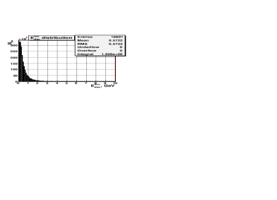
a) b)

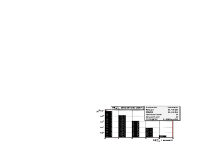
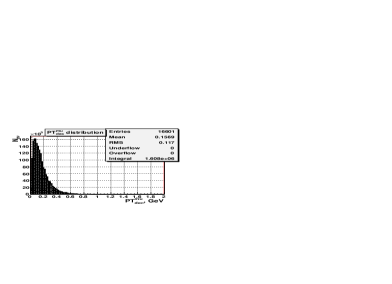
c) d)

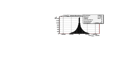
e) f)

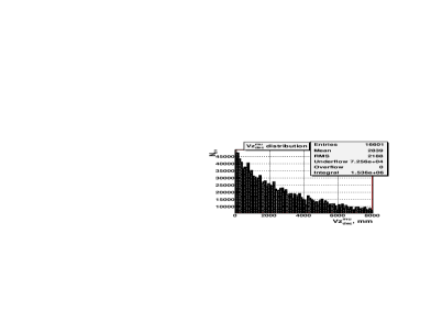
Figure 16: Left column: distributions of the number of decay muons versus their a): the energy $E^{\mu}_{dec}$; c): transverse momentum $PT^{\mu}_{dec}$ and e): polar angle $\theta^{\mu}_{dec}$. Right column: distributions of b): the total number $N^{\mu}_{bkg}$ of fake muons per the signal event; d): x coordinate of the fake muon production vertex and f): z coordinate of the fake muon production vertex

The distribution of a number of muon signal events versus a number of fake decay muons $N^{\mu}_{bkg}$, contained in each event, is shown in the plot b. It is seen that there can be up to 4 muons in the final state. From the first bin of this plot one may see that about $83\%$ of events have no background fake muons at all. This value agrees well with the number of entries shown in the plot a which was discussed above. The amount of events free of fake muons does not corresponds to the previously discussed amount of the events without charged pions because of applied restriction of the decay volume. It is also seen from the plot b that the numbers of events with one fake muon, with two and three fake muons are about by, respectively, one, two and three orders less than the number of events without any fake muon.

The left column of Fig.16 includes (from top to bottom) the energy $E^{\mu}_{dec}$, transverse momentum $PT^{\mu}_{dec}$ and polar angle $\theta^{\mu}_{dec}$ distributions of muons which appear from hadron decays. From comparison of these plots with their analogs from Fig.2, i.e. of those which are done for the signal muons, one may see that the fake muons are less energetic than the signal ones. One may also find that the mean value of the signal muons energy (see plots a, b of Fig.2) $<E^{\mu}>$ = 2.6 GeV corresponds to such a point in the energy spectrum of fake muons which decay in the restricted volume, where the contribution of fake muons (in the same signal events) is very low. Analogously, the mean value of the PT-distribution of signal muons $<PT^{\mu}_{signal}>=0.7$ GeV (see Fig.2) corresponds to that point where the spectrum of $PT^{\mu}_{dec}$ practically vanishes.

Therefore, one has to look for the set of some reasonable cuts (chosen with an account of the real detector effects) on a muon energy $E^{mu}$ as well as on its $PT^{mu}$ value, which may lead to an essential reduction of decay muons contribution and to keep at the same time the main part of signal events. For example, the comparison of the plots a and c of the Fig.2 with the analogous plots in Fig.16, leads to a conclusion that the cuts $E^{\mu}>0.2$ GeV, $PT^{\mu}>0.2$ GeV may allow to get rid of about $66\%$ of decay muons in the signal events and to save the most of signal (i.e. belonging to signal $\mu^{+}\mu^{-}$- pair) slow and fast muons. We shall return to this problem a bit later.

Another way which may help to discriminate the signal muons from the ”decay” ones is to use the information about the position of fake muon production vertex and the reconstruction of the invariant mass of the parent and grandparent hadrons. The plots d and f of Fig.16 contain the distributions of Vx- and Vz- (z-axis is chosen along the beam direction) components of the 3-vector $V=(Vx,Vy,Vz)$, which gives the position of a fake muon production vertex in millimeters (mm) Let us note that these plots are obtained within the PYTHIA level of simulation, i.e. without an account of details of detector construction and the effects caused by the magnetic field. Withing this approximation the distributions of Vx- and Vy- components have to be similar. For this reason, we shall show in the following only the distribution of Vx- component. Seen from the Fig.16 the Vz component of about $3-5\%$ of events may be rather close to zero, i.e. to the interaction point. The corresponding fake muons, produced near the interaction point, may give rise to the most difficult background. The contribution of the background muons from the other type of events (based mainly on minimum bias and QCD partonic subprocesses) will be discussed in the following Section 7.

6.4 Fake electrons

Now let us consider the situation with fake decay electrons and positrons background in the case of signal processes based on the quark level subprocess of electron-positron pair production . Fake electrons produced in these decays will be also called in the following as “decay” ones. Recall, as it was already mentioned in the Section 2 and in the begining of the present one, that we shall use the sample of 100000 generated signal events with $e^{+}e^{-}$ production.

Fig.17a presents the contribution of different parent particles into the process of creation of the fake electrons. It clearly demonstrates that among all shown sources of fake electrons the contribution of neutral pion $\pi^{0}$ decay (bin 2) is a dominat one. It provides a much higher (about of one order) contribution than all of other decay channels. The electrons/positrons may appear in neutral pion decay only through the channel of Dalitz decay into a photon and an electron-positron pair: $\pi^{0}\rightarrow\gamma+e^{+}e^{-}$. The next contribution, which is by about one order less, give, in decending order, muon (bin 1), $\eta$- and K-mesons decays as well as the decay of $\Lambda^{0}$. Neutral pions in their turn may arise from decays of $\eta$- and $\omega$-mesons or heavier mesons and baryons, produced as resonance states according to the LUND fragmentation model.

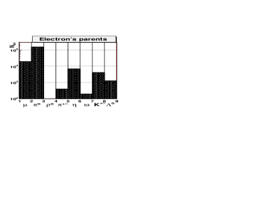
a) b)

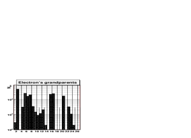
Figure 17: Distributions of: a) parents of fake $e^{+}/e^{-}$; b) grandparents of fake $e^{+}/e^{-}$

Fig.17 b shows the distribution of a number of background electrons versus the type of their grandparents. The correspondence between the bin numbers shown on the x-axis and the name of the grandparent particle can be found from the left column of the Table 7 of Appendix: (Tables which are presented in the Section 11). From comparison with this Table one can see that the strings (bin 2) are the main source of electron parents. Then follow a group of $\rho$-, $\eta$- and $\omega$-mesons (bins 5-7) as well as the group of $\Delta$-resonances (bins 15-16) and $\Lambda^{o}$ (bin 20). Two orders less contribution is provided by the group of kaons (bins 8-11) which is followed by $\eta^{{}^{\prime}}$ resonance (bin 12) and the group of $\Sigma$-resonances (bins 22-24).

The plots, containing the distributions of the fake decay electrons which appear in signal events (based on the $q\bar{q}\to e^{+}e^{-}$ subprocess) are presented in Fig.18. They are done basing on the sample of 100 000 generated by PYTHIA signal events which were discussed in the Section 2 and contain signal $e^{+}e^{-}$ pairs. Like in previouse subsection we use here the same restriction on the detector volume.

a) b)

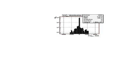
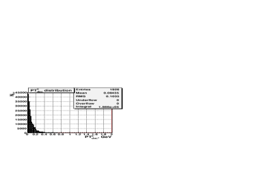
c) d)

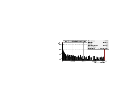
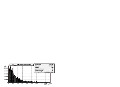
e) f)

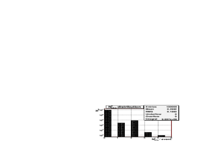
Figure 18: Left column: distributions of the number of decay electrons versus their: a):the energy $E^{e}_{dec}$; c): transverse momentum $PT^{e}_{dec}$ and e): polar angle $\theta^{e}_{dec}$. Right column: distributions of b): the total number $N^{e}_{bkg}$ of fake muons per the signal event; d): x coordinate of the fake $e^{+}/e^{-}$ production vertex and f): z coordinate of the fake $e^{+}/e^{-}$ production vertex

From the statistics frame in the upper part of plots one may see that in a case of decay electrons the number of entries is 1926 (i.e. the fraction of the signal processes which includes fake electrons is about $2\%$).

The comparison of the energy $E^{e}_{dec}$ and transverse momentum $PT^{e}_{dec}$ distributions of fake electrons in signal events, which are given in the left-hand column of Fig.18, with the analogous plots for fake muons from the left-hand column of Fig.16, allows to conclude that in electron case the distributions fall at least twice steeply than in muon one.

Analogously with the previous subsection, the comparison of the same $E^{e}_{dec}$ and transverse $PT^{e}_{dec}$ distributions of fake electrons in signal events, shown in plots a and c of Fig.18, with the plots a and c of Fig.2 for signal electrons leads to the conclusion that the soft cuts like $E^{e}>0.2$ GeV and $PT^{e}>0.2$ GeV may allow to eliminate the most of fake electrons at the cost of about $10\%$ loss of signal events.

The right-hand column of Fig.18 includes plots b and d. They contain the values of the Vx- and Vz- components of the 3-vector V which points the position of electron production vertex. In contrast to the form of vertex distribution for muon production case (see the plot d in Fig.16), the concentration of Vz-component of electron production (see plot d in Fig.18) near the interaction point poses the essential difference of a $e^{+}e^{-}$ channel as compared to a case of $\mu^{+}\mu^{-}$ channel. In the last case, the most of background muons are produced by light charged pions which may decay in flight at a rather large distance from the interaction point. It is also seen from plot f in Fig.18 and the analogous plot a in Fig.16 that the number of fake electrons or fake muons in signal events may be up to four in both cases.

6.5 Cuts for fake leptons reduction in signal events

The analysis of distributions discussed above leads to the conclusion that the following cuts:

$\bullet$ 1) we select the events with the only two leptons with $E_{l}\geq$ 0.2 GeV, $PT_{l}\geq$ 0.2 GeV;

$\bullet$ 2) the charges of these two leptons must be of the opposite sign;

$\bullet$ 3) the vertex of lepton origin lies within the range $R_{vtx}\leq$ 15 mm from the interaction point;

which, being applied to the sample of signal events, can allow one to select a subsample which include a strongly reduced fraction (fr) of events containing fake leptons ($fr_{e}=0.008\%$ for the case of electron pair production and $fr_{\mu}=0.001\%$ for the muon pair production). The loss of the signal events due to application of cuts 1)–3) is shown in Table 3.

Table 3: Loss of the signal events (in $\%$) after application of cuts 1)–3)

N of cuts	$e^{+}e^{-}production$	$\mu^{+}\mu^{-}production$
1	$14.330\%$	$16.525\%$
1 $\&$ 2	$14.340\%$	$16.805\%$
1 $\&$ 2 $\&$ 3	$14.341\%$	$17.108\%$

One can see from this Table that it is possible to select the signal events which are almost free of background fake leptons at the cost of diminishing of the signal events sample by $\approx$ 17 $\%$ for $\mu^{+}\mu^{-}$ and $\approx$ 14$\%$ for $e^{+}e^{-}$ production.

7 QCD and minimum-bias background events

The other source of the background is the leptons produced in the minimum-bias (low - $P_{T}$ and diffractive scattering) events and QCD background these are mainly $q+g\rightarrow q+g$, $g+g\rightarrow g+g$ and $q+q^{\prime}\rightarrow q+q^{\prime}$) processes, where the possibility of appearance of two (and more) leptons in the final state is very high. For analysis of these processes $10^{6}$ events of antiproton diffraction over proton target with $E_{beam}=$14 GeV were generated with PYTHIA 6.4. These events include mentioned above processes, including the signal one $\bar{q}+q\to l^{+}l^{-}$. According to PYTHIA the total cross section of these processes $\sigma^{bkg}_{tot}=50.17$mb is about $10^{7}$ times higher than the cross section of the signal MMTDY subprocess $q+\bar{q}\rightarrow l^{+}+l^{-}$: $\sigma^{\bar{q}q\to l^{+}l^{-}}=5.57\cdot 10^{-6}$mb. In the following subsections 7.1-7.2 we shall present the distributions obtained without use of any cuts.

7.1 Muon background.

The distribution of the parents of muons produced in background minimum-bias and QCD events is presented in Fig.19 a. It is seen that, like in a case of fake muons in signal events (see Fig. 14 a), the main contribution comes from $\pi^{\pm}$- and $K^{\pm}$-meson decays. Fig.19 b shows the distribution of muons grandparents. One can see (using the right-hand column of Table 7 of the Section 11 (Appendix: Tables) that the main grandparents of muons in QCD and minimum-bias events are the clusters and strings (bins 1, 2) as well as the $\rho$-, $\eta$- and $\omega$-mesons (bins 3-6). Then follow the $\Delta$-resonances (bins 16, 17) and $\Lambda^{0}$ (bin 20).

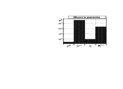
a) b)

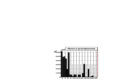
Figure 19: Distributions of: a) parents of background $\mu^{+}/\mu^{-}$; b) grandparents of background $\mu^{+}/\mu^{-}$

The kinematical and other distributions of muons produced in the above mentioned generated background minimum-bias and QCD events are shown in Fig.20 It is seen that the kinematical distributions (plots b, c, e) do not differ so much (that is natural) from those of fake “decay” muons produced in the signal $p\bar{p}\rightarrow l^{+}l^{-}+X$ processes (see Fig.16).

a) b)

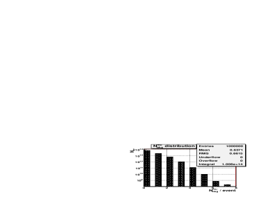
c) d)

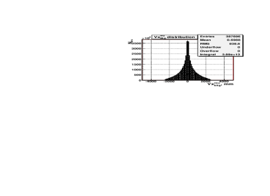
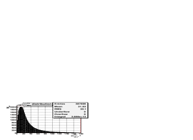
e) f)

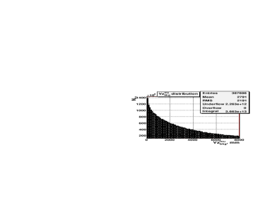
Figure 20: Left column: distributions of the number of background muons versus a): energy $E^{\mu}_{bkg}$; c): transverse momentum $PT^{\mu}_{bkg}$ and e): polar angle $\theta^{\mu}_{bkg}$. Right column: distributions b): of the total amount $N^{\mu}_{bkg}$ of muons per event; d): x coordinate of the background muon production vertex and f): z coordinate of the background muon production vertex

The distribution of the number of generated background events versus the amount of fake muons produced per event, i.e. $N^{\mu}_{bkg}$, is shown in plot b) of Fig.20. It differs noticeably from its analog shown in Fig.16 which contains only the distribution of fake ”decay” muons in signal lepton pair production events. The number of muons in the final state, contained in one and the same background event, can be up to 7. It means that the probability of production of the pair of fake muons with the charges of the opposite signs (like in signal events) is rather high in these background events. Such pairs may fake quite well the signal events.

The distribution plots of the production vertexes of background muons are shown in the right column of Fig.20. It is seen from the plot f of Fig.20 that the most of the muon production vertexes are spread over detector volume while for some of events these vertexes are rather close to the interaction point. So the information about the vertex position can be useful for background separation.

7.2 Electron background

Let us consider now the case of electrons produced in the background minimum-bias and QCD events. The distribution of the parents of background electron in the discussed above sample of minimum-bias and QCD events is presented in Fig.21 a. It is seen that, like in a case of fake electrons in signal events (see Fig. 17 a), the main contribution comes from $\pi^{0}$-, $\eta$-, charged $K$-mesons (bins 2, 5 and 7, respectively) and also from muon decays (bin 1). The main source of fake electrons are decays of neutral pions ($\pi^{0}\rightarrow\gamma+e^{+}e^{-}$). They can appear directly or from decays of $\rho$-, $\eta$-, $\omega$- , K- mesons, as well as from $\Delta$- resonances decays.

From the Fig.21 b one may see that in the minimum-bias and QCD events sample the structure of the distributions of electron grandparents is rather

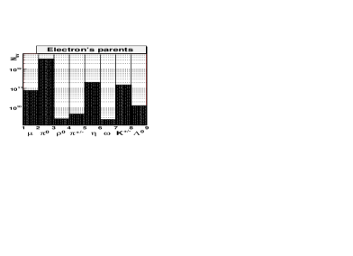
a) b)

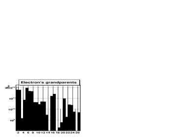
Figure 21: Distributions of: a) parents of background $e^{+}/e^{-}$; b) grandparents of background $e^{+}/e^{-}$

different from its analog presented in Fig.17 b for a case of fake electrons in the sample of signal events with the signal electron-positron pairs. Namely, different to the plot Fig.17 b the charged $\rho$-mesons (bin 5) takes the dominant position in the plot Fig.21 b. Then follows the noticeably increased contribution of clusters (bin 1) which height reaches the height of strings contribution (bin 2). It is also seen that on total the contribution of light vector mesons ($\rho$, $\eta$ and $\omega$ (bins 5-7)), as well as the contribution of K- (bins 8-11) and $\eta^{{}^{\prime}}$-, $\phi$- mesons (bins 12,13), have grown up as comparing to the higher bins (15, 16 and 20), which correspond to $\Delta$- and $\Sigma$- barions, respectively.

a) b)

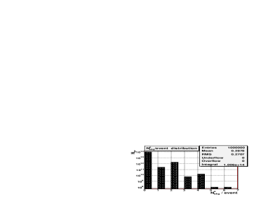
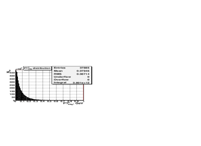
c) d)

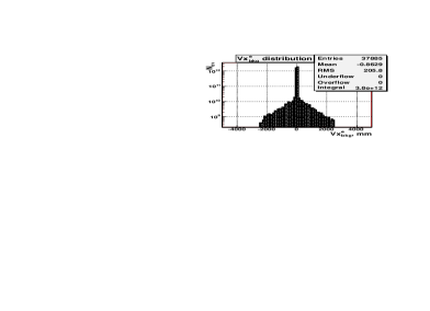
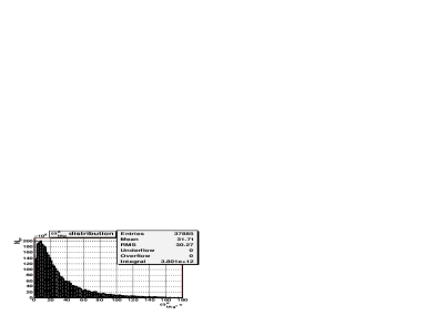
e) f)

Figure 22: Left column: distributions of the number of background electrons versus a): the energy $E^{e}_{bkg}$; c): transverse momentum $PT^{e}_{bkg}$ and e): polar angle $\theta^{e}_{bkg}$. Right column: distributions b): of the total amount $N^{e}_{bkg}$ of electrons per the background event; d): x coordinate of the background $e^{+}/e^{-}$ production vertex and f): z coordinate of the background $e^{+}/e^{-}$ production vertex

The distributions obtained from the sample of mentioned above generated minimum-bias and QCD background events, are shown in Fig.22. The kinematical distributions (plots a, c and e) are rather similar to the distributions of fake decay electrons in the signal events which were discussed in the subsection 6.4 and presented at Fig.18. From Fig.22 one may see that the total number of electrons in the sample of generated 1000000 minimum-bias and QCD events is equal to 37885. This number is of order less than the number of fake muons produced in the same sample of $10^{6}$ minimum-bias and QCD events (see previous subsection 7.1). Plot b) of Fig.22 shows the distribution of the number of generated minimum-bias and QCD events versus the number of decay electrons per event. The third bin in this plot, as well as the other bins to the right from it, show how many events may contain two and more electrons. In these events there may appear the $e^{+}e^{-}$-pairs, which potentially may fake the signal events. It is clearly seen that the probability of appearance of 2 and more electrons in the final state reduces to a value of about few percents of the total number of generated events.

The plots d and f of Fig.22 show the distributions of the position of the electron production vertex in the background sample in the transversal ($Vx^{e}_{dec}$) and the longitudinal ($Vz^{e}_{dec}$) directions. It is seen that the most of background electrons, originating from hadron decays, are produced near the interaction point ($V_{x}=0$ and $V_{z}=0$), like it take place in Fig.18.

8 Background separation

To reduce the background contribution from the minimum bias and QCD events we added two new cuts to the previously used cuts 1)-3) (see Section 6.5). Finaly, we use the following selection cuts:

$\bullet$ 1.) the events with the only two leptons with $E_{l}\geq$ 0.2 GeV, $PT_{l}\geq$ 0.2 GeV;

$\bullet$ 2.) the charges of these two leptons must be of the opposite sign;

$\bullet$ 3.) the vertex of lepton origin lies within the radius $R_{vtx}\leq$ 15mm

from the interaction point;

$\bullet$ 4.) $M_{inv}(l^{+},l^{-})\geq$ 0.9 GeV;

$\bullet$ 5.) lepton isolation criteria: the summed energy E_sum of all the particles around

the lepton within the cone of the radius R=$\sqrt{\Delta^{2}_{\varphi}+\Delta^{2}_{\eta}}$ = 0.2 in the $\eta-\varphi$ space

is not higher than E${}^{max}_{sum}=0.5$ GeV .

Here $\Delta_{\varphi}=\varphi_{l}-\varphi_{p}$ is the difference of the lepton’s (l) azimuth angle $\varphi_{l}$ and the azimuth angle $\varphi_{p}$ of the particle (p), contained within the cone of the radius R around the lepton. Analogously, $\Delta_{\eta}=\eta_{l}-\eta_{p}$ is the difference of the lepton and the particle pseudorapidities.

Few words are in order now about the choice of the last two cuts. Tables 4 and 5 show, for muon pair and electron pair production cases, respectively, the influence of the variation of the cut on dilepton invariant mass $M_{inv}(l^{+},l^{-})$ on the loss of signal events and the value of signal to background ratio S/B (after application of the cuts 1.)-3.). It is seen from Table 4 that in $\mu^{+}\mu^{-}$ case the growth of the maximal value of $M_{inv}(l^{+},l^{-})$ up to $M_{inv}(l^{+},l^{-})=1.2$ GeV allows to get rid completely of the background at cost of loosing of 35 $\%$ of signal events, while in $e^{+}e^{-}$ case, see Table 5, the same upper limit leads only to S/B$=$ 2.3.

Table 4: Efficiency of the $M_{inv}^{l^{+}l^{-}}$ cut for the case of $\mu^{+}\mu^{-}production$

$M_{inv}^{\mu^{+}\mu^{-}}\geq$ (GeV)	S/B for	Efficiency	The rest of signal events
0.9	0.12	0.0805	85$\%$
1.0	0.22	0.0444	82$\%$
1.03	0.50	0.0198	81$\%$
1.05	0.69	0.0136	78$\%$
1.1	1.50	0.0063	76$\%$
1.2	BKG = 0	0	65$\%$

Table 5: Efficiency of the $M_{inv}^{l^{+}l^{-}}$ cut for the case of $e^{+}e^{-}production$

$M_{inv}^{e^{+}e^{-}}\geq$ (GeV)	S/B for	Efficiency	The rest of signal events
0.9	0.093	0.0059	84$\%$
1.0	0.146	0.0035	81$\%$
1.03	0.375	0.0014	78$\%$
1.05	0.395	0.0012	74$\%$
1.1	0.762	0.0006	69$\%$
1.2	2.3	0.0002	61$\%$

The results of all the five cuts sequent application to the sample of inelastic $\bar{p}p\to X$ events which contains the minimum-bias and QCD events (incuding the signal events based on the parton level annihilation subprocess ${q\bar{q}\to\gamma^{*}\to l^{+}l^{-}}$ ) are collected in the Table 6. It is seen that the first three cuts allow to enlarge the the S/B ratio by about one order in a case of muon pair production. At the same time, the third cut is inefficient for the case of $e^{+}e^{-}$-pair production. The forth cut $M_{inv}(l^{+},l^{-})\geq$ 0.9 GeV allows to increase the S/B ratio in $e^{+}e^{-}$ case by more than two orders and by about three ordes the S/B ratio for $\mu^{+}\mu^{-}$ case.

Table 6: Cuts influence for background events.

N of cuts	S/B for $\mu^{+}\mu^{-}production$	Efficiency	S/B for $e^{+}e^{-}production$	Efficiency
1	1.41 $\cdot 10^{-5}$	0.007	5.34 $\cdot 10^{-4}$	1.78 $\cdot 10^{-4}$
2	2.12 $\cdot 10^{-5}$	0.665	5.41 $\cdot 10^{-4}$	0.98
3	9.94 $\cdot 10^{-5}$	0.002	5.47 $\cdot 10^{-4}$	0.99
4	0.123	0.08	9.27 $\cdot 10^{-2}$	0.006
5	Background = 0	–	3.8	0.024

The plots presented in the Figs.23, 24 are done to illustrate the action of the lepton isolation criterion used in the definition of the fifth cut. They show the distributions of the total energy of the particles which are contained within the cones of the radius R around the leptons. Figures 23 and 24 present these distributions for the electron and muon cases, correspondingly. By comparing the plots a (for leptons from the signal events) with the plots b (for background leptons from minimum-bias and QCD events) one can easily see that the signal events have much smaller summarized energy content within the cone of $R\leq 0.2$ than the energy content in background events. This observation is used in the cut 5.

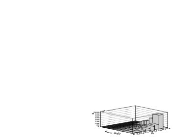
a) b)

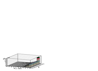
Figure 23: Lepton isolation for the e case. Distributions of the summarized energy $E_{sum}$ within the cone of the radius R=0.1, 0.2, 0.3…. : a) signal events, b) background events.

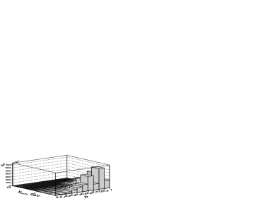
a) b)

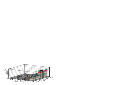
Figure 24: Isolation for the $\mu$ case. Distributions of the summarized energy $E_{sum}$ within the cone of the radius R=0.1, 0.2, 0.3…. : a) signal events, b) background events.

From the Table 6 one can see that the last cut on the lepton isolation, i.e. the choice of only those final state leptons which have the restricted value of the summarized energy (not greater than $E_{sum}$=0.5 GeV) of other particles contained within the cone of some fixed radius R$=\sqrt{\varphi^{2}+\eta^{2}}=$NR (NR$=0.1,0.2,0.3...$) around the direction of the lepton 3-momentum, allows one to achieve (choosing NR$=0.2$) the value of the signal to background ratio equal to S/B = 3.8 for electron production case and completely to get rid of background in muon production case. In both cases the application of the fifth cut leads to additional 8$\%$ loss of the signal events left after application of the first four cuts. Let us note that the same criteria, but with the use of a more restricted form of the forth cut $M_{inv}(e^{+},e^{-})\geq$ 1.0 GeV, allows to increase the signal to background ratio up to S/B = 9 in $e^{+}e^{-}$ case.

9 Remarks on the possibility of measuring the multi-parton interactons and the intrinsic quark transverse momentum in the proton.

In addition to the opportunity to get the information about parton distribution functions, which was already discussed in Section 5, let us also mention here three other ones which may be useful for studying quark dynamics in proton and its PDFs.

The first two are connected with the processes of two

$$\bar{p}p\rightarrow l_{1}^{+}l_{1}^{-}+l_{2}^{+}l_{2}^{-}+X$$ (4)

or even three lepton pairs

$$\bar{p}p\rightarrow l_{1}^{+}l_{1}^{-}+l_{2}^{+}l_{2}^{-}+l_{3}^{+}l_{3}^{-}+X$$ (5)

production in one event.

Both of these processes can include two and three quark annihilation $q\bar{q}\rightarrow l^{+}l^{-}$ subprocesses, respectively. The total cross sections of such processes can be smaller as compared to the $\bar{p}p\rightarrow l^{+}l^{-}+X$ process which includes a single $q\bar{q}\rightarrow l^{+}l^{-}$ subprocess. Nevertheless, they may contain interesting physical information which can be more easily extracted at the intermediate energies than at the higher ones.

First, the measurement of the characteristics of the system of other than lepton pairs particles, produced in the process (4), will give us the opportunity to get the information about the so-called ”underlying” event. The study of the analogous distribution in the process (5), in which all valence quarks (and antiquarks) in proton (and antiproton) will annihilate into lepton-antilepton pairs, may provide the information about gluon content in the proton. The understanding of the physics of the ”underlying” event, i.e. the interaction of partons which do not participate in the hard subprocess $q\bar{q}\rightarrow l^{+}l^{-}$, is very important for the interpretation of the results of the present Tevatron and future LHC experiments.

The second opportunity, also provided by the processes (4) and (5), is the study of the so-called multiple parton hard interaction processes in pp- and $p\bar{p}$ interactions which are widely discussed in connection with the problem of a proper account of background contribution to the processes which are planned for seaches of the New Physics signals at Tevatron and LHC. It is worth mentioning that the measurements of the proceses (4) and (5) can be done for the case when final state lepton pairs would have different flavor, like $\bar{p}p\rightarrow e^{+}e^{-}+\mu^{+}\mu^{-}+X$. In such case we shall have the situation when four hadronic jets events, used in previous measurements of multiple interactions [22]-[24], are substituted by events withfour leptons. This substitution shall increase the precision of measurement of the parameters of multiple interections as it was shown in recent measurements done with ”3jet + photon” final states [25], [26].

Besides getting the information about the fraction of multiple interactions their study opens the possibility to get the information about the spatial distribution of quarks within the proton. It is obvious that in a case of uniform distribution of quarks within the proton volume the occurrence of the first parton-parton interaction would not influence on the probability of happening of the second interaction, while in a case when the quarks are concentrated in small region the probability of happening of the second interaction becomes higher if one of the quarks has taken part in the first interaction.

The third opportunity is connected with the possibility to measure the characteristics of internal quark motion in the proton. This possibility is based on the fact that the shape of the distribution of the modulus of the vector sum of quark and antiquark transverse momentum vectors

$$P^{q\bar{q}}_{T}=|\vec{P}^{q\bar{q}}_{T}|=|\vec{P}^{q}_{T}+\vec{P}^{\bar{q}}_{T}|$$ (6)

practically coincides (due to the transverse momentum conservation law) with the shape of the above-considered distribution of the modulus of the lepton pair transverse momentum $P^{l^{+}l^{-}}_{T}$, shown in the plot b of Fig.12.

The variable $P^{q\bar{q}}_{T}$ is of special interest because it contains the information about two important physical features of quark dynamics inside the hadron. Indeed, in our case when a beam antiproton is directed along the z axis and it scatters over the proton fixed target, there may be only two sources of transverse motion of quarks in the initial state :

A) internal Fermi-motion of quarks (with some transverse velocity) inside a proton, i.e. the so-called ”$k_{T}$-effect”;

B) initial-state radiation (ISR) of gluons or photons from quarks before hard quark-antiquark annihilation;

The importance of these two effects was recently discussed [33] in connection with the interpretation of prompt photon production study in the experiment E706 at Fermilab [27] and also with the study of ”${\gamma/Z+jet}$” events, which are sensitive to the shape of gluon distribution, at the LHC [29] and Tevatron [30], [31].

10 Conclusion.

The modeling of dilepton production in antiproton scattering over proton target $\bar{p}p\rightarrow l^{+}l^{-}+X$ is done for the intermediate energy $E_{beam}=14$ GeV on the basis of PYTHIA event generator and the parton level subprocess of quark-antiquark annihilation $\bar{q}q\rightarrow l^{+}l^{-}$.

The distributions of most essential kinematical variables of individual leptons, are are presented in Section 2. They show that the energy and angle spectra of the fast (most energetic) leptons in a pair are very different from those of slow leptons: the mean value $<{E^{l}_{fast}}>=3.85$ GeV is about three times higher than that one of slow leptons $<{E^{l}_{slow}}>=1.36$ GeV. The simulation has also shown a tendency which may be a rather general one: fast leptons fly predominantly at smaller angles $<{\theta^{l}_{fast}}>=16.5^{o}$ as compared to the angles of slow ones $<{\theta^{l}_{slow}}>$= $38.2^{o}$. It is worth noting that about $6\%$ of events may have slow leptons, that may scatter into the back hemisphere, i.e. ${\theta^{l}_{slow}}>90^{o}$. The angle-energy, energy-energy and angle-angle correlations among a slow and a fast lepton in the same lepton pair in event are also described in Section 2 and are presented in Figs.4, 5 together with the corresponding distributions of the number of events versus the corresponding lepton energies and angles.

These distributions allow one to estimate the energy, transverse momentum and angle ranges that may be covered by leptons produced in quark-antiquark annihilation process. They were useful for proper design of muon system and may be also used for the electromagnetic calorimeter. Tables 1 and 2 show the estimation of the loss of signal events depending on the choise of cuts on the lower values of lepton energy and, respectively, on the upper limit of the angle size of the muon system and the electromagnetical calorimeter. From these Tables one can see that, for instance, the choise of cuts $E^{min}_{cut}=0.5$ GeV and $\theta^{l}_{max}=90^{o}$ results in about 30$\%$ loss of signal events. The simulation PYTHIA has shown that one may expect to gain about $7\cdot 10^{7}$ MMTDY events per year for the luminosity $L=2\cdot 10^{5}mb^{-1}s^{-1}$.

The analogous study was done on the basis of PYTHIA in the Section 3 for the leptons which may appear in decay of J/$\Psi$ mesons, produced in the benchmark process $\bar{p}p\rightarrow J/\Psi+X$. It was shown that the leptons, produced in J/$\Psi\rightarrow l^{+}l^{-}$ decay, fit well into the same angle regions as the leptons produced in MMTDY process $\bar{p}p\rightarrow l^{+}l^{-}+X$. The reconstruction of the lepton pair invariant mass can allow to get rid of background without a sizable loss of signal events.

In Section 4 the study of kinematical characteristics of lepton pair as a whole system was done. It is shown that the spectrum of the invariant mass of the lepton pair decreases rather fast and vanishes at $M^{l{+}l{-}}_{inv}=2.5$ GeV. At the same time the lepton pairs total energy $E^{l^{+}l^{-}}$ spectrum starts at around 1 GeV and extends up to the value of 12 GeV. It is also demostraited that about a half of the events have the lepton pair energy higher than 5 GeV. It is shown that one can expect that in about 50$\%$ of events the lepton pairs would be rather energetic and they can take away from 33$\%$ up to 80$\%$ of the total energy of the final state system. The square of the invariant mass $(M_{inv}^{l^{+}l^{-}})^{2}=Q^{2}=q^{2}=(P^{l^{+}}+P^{l^{-}})^{2}$ has the meaning of the square of the momentum transfered from the hadronic system of quark-antiquark pair to the electromagnetic system of final state dilepton pair.

In Section 5 the analysis of distributions, obtained by PYTHIA, allowed to determine the region in x-Q²-plane which can be available for measuring the proton structure function at PANDA. This region is defined by the following boundaries: $0.05\leq x\leq 0.7$ and $Q^{2}\leq 6.25$ GeV. Let us emphasize that the measurements in this region of positive (”time-like”) $q^{2}\equiv(P^{l^{+}}+P^{l^{-}})^{2}=Q^{2}\geq 0$ would be a good extension of studies planned to be done at JLab in the region of negative (”space-like”) values of $q_{dis}^{2}=(P^{l}_{in}-P^{l}_{out})^{2}\leq 0$.

An important problem of background suppresion is considered in Sections 6, 7 and 8. In Section 6 we have concentrated on the fake leptons which can appear from hadron decays in the same signal process. We studied signal processes with dimuon production separately from the processes with electron pair production using for this two separate event samples with signal muon pair and, respectively, electron pair production. First we have considered the case of $\mu^{+}\mu^{-}$ production. The histograms which demonstrate the relative contribution of different parents and grandparents of produced muons are presented in the subsection 6.1. It is shown that charged pion decays produce the main part of fake muons. The next dominant source is the decays of charged K-mesons (its contribution is by more than two ordes less than that one from pions).

Some details about pion source are presented in the subsection 6.2 where it was shown that about 42$\%$ of signal events do not contain at all any charged pions, while 24$\%$ of them contain only one pion and 27$\%$ include two charged pion in the final state. About 5$\%$ of signal events include tree charged pions and 1.5$\%$ have four charged pions. This prediction of PYTHIA indicate that the reconstraction of invariant masses of parent and grandparent hadrons can be a quite reliable way for fixing the origin of produced fake muons.

The kinematical plots, shown in subsection 6.3 (and in subsection 6.4 for fake electrons) are done by applying a geometrical restriction on the detector volume. This restriction produced a strong reduction of the fraction of fake leptons. In result the energy and transverse momentum spectra of fake muons became essentialy shorter than their analogs shown in the Section 2. The fraction of signal events which include fake muons has reduced down to about 16.6$\%$ (in comparison with pion distributions). It means that, according to PYTHIA, about 83$\%$ of signal events would not contain fake muons at all due to the used restriction of the decay volume. The analogous parent, grandparent and kinematical distributions were obtained in subsection 6.4 for a case of background electrons. It is found that the application of geometrical restriction on the detector volume provides the reduction of signal events fraction (containing fake electrons) down to 2$\%$.

The set of three cuts are proposed in the subsection 6.5 which, being applied together with the mentioned above restriction on the detector volume, allows a further reduction of the fraction of the signal events containig fake decay leptons. Namely, they are: $fr_{\mu}=0001\%$ in a case of $\mu^{+}\mu^{-}$ production and $fr_{e}=0.008\%$ in $e^{+}e^{-}$. Let us underline that this strong reduction of the fraction the signal events including fake leptons was achieved at the cost of the loss of a noticeable number of selected signal events. These losses are: $\approx 17\%$ for $\mu^{+}\mu^{-}$ and $\approx 14\%$ for $e^{+}e^{-}$ production.

Much more dangerous background, provided by minimum-bias and QCD events, was studied in the Sections 7 and 8. The former includes two subsections in which the figures with parent and grandparent relative contributions as well as the with kinematical distributions for $\mu^{+}\mu^{-}$ and $e^{+}e^{-}$ cases are presented, respectively. Subsection 8 contains the set of five cuts which include three cuts which were previously used to reduce the number of events containing fake decay leptons. The fourth cut reduces the spectrum of the invariant mass of dilepton system by the condition $M_{inv}(l^{+},l^{-})\geq 0.9$ GeV, while the fifth cut uses the isolation criteria for the lepton. It is shown that dispite the fact that the cross section of minimum-bias process $\sigma^{minbs}_{tot}$ is by about 7 oders larger than the cross section of the signal process $\sigma^{\bar{q}q\to l^{+}l^{-}}_{tot}$ the application of these five cuts allows to get rid completely of minimum-bias and QCD background contribution in $\mu^{+}\mu^{-}$case and to reach the value of S/B = 3.8 for $e^{+}e^{-}$ case. It is worth mentioning that the application of the fourth and the fifth cuts leades to an additional loss of the number of selected signal events by 8$\%$.

The Section 9 contains three important remarks about the physical potential of studing events having several lepton-antilepton pairs in the final state. First, it is stressed that the study of events with two (and, maybe, even three) lepton pairs would allow to enlarge the precision of the parameters of multiple quark interactions. It will also essentialy extend the region of QCD studies because up to now there were done only five dedicated measurements of such events in proton-proton and antiproton-proton collisions. The first three processes considered the case when four jets were produced in the final state, while the last two measurements have used the events in which the final state was including tree jets plus one direct photon. Therefore, the measurements in which the jets would be substituted by leptons would allow to reach a higher level of precision.

It was also noted that at the same time such events, based on the processes of valence quarks annihilation in the colliding protons, will provide a clean information about the dynamics of spectator quarks interactions, i.e. about the so-called ”underlaying events”. It is worth mentioning that the most interesting would be the measurements with three leptons pairs production, because in this case the underlaying processes would be defined mostly by soft gluon interactions.

The third opportunity, which was discussed in the Section 8, can be based on the measurement of the transverse momentum of lepton pair which is directly connected with the transverse momentum of the system of two annihilating quarks. The latter can be caused by the so-called ”$k_{T}-effect$” which is connected with the so called ”Fermi-motion” of quarks inside the proton or the radiation of gluons by initial-state quarks. This information is of a big interest for the interpretation of QCD effects observed at high energy hadron colliders.

It should be underlined that the present PYTHIA simulation does not take into account the detector effects (like the magnetic field and the material of the apparatus, for example). Hence, the obtained plots, which describe the unbiased distributions of the produced free particles, may be mainly useful for preliminary estimations and working out the criteria (cuts) for selection of experimental events for further physical analysis. The detailed GEANT simulation with account of detector design (and based on the simulated PYTHIA event sample described here) will be a subject of our following publication. Nevertheless, one can expect that there is a high probability that the main features of the real process, corrected to detector effects, would be rather similar to those shown in the plots presened in this article.

11 Acknowledgements.

One of the authors (A.N.S.) acknowledge support from Russian-German ”FAIR Russia Research Centre“ (which is also supported from Russian Federal Agency for Atomic Energy ”Rosatom“ and German Helmholtz Association).

12 Appendix: Tables.

Table 7: Bin correspondence to the particle names for the case of e’s and ${\mu}$’s grandparents.

Bin number	Name of e’s grandparent particle	Name of $\mu$’s grandparent partticle
1	cluster	cluster
2	string	string
3	$\rho^{0}$	$\rho^{0}$
4	$\pi^{+}$	$\rho^{+}$
5	$\rho^{+}$	$\eta$
6	$\eta$	$\omega$
7	$\omega$	$K^{0}_{S}$
8	$K^{0}_{S}$	$K^{*0}$
9	$K^{*0}$	$K^{+}$
10	$K^{+}$	$K^{*+}$
11	$K^{*+}$	$\eta^{\prime}$
12	$\eta^{\prime}$	$\phi$
13	$\phi$	$\Delta^{-}$
14	$\Delta^{-}$	$\Delta^{0}$
15	$\Delta^{0}$	$K^{+/-}$ like string
16	$\Delta^{+}$	$\Delta^{+}$
17	$K^{+/-}$ like string	$\Delta^{++}$
18	$\Delta^{++}$	$\Sigma^{-}$
19	$\Sigma^{*-}$	$\Sigma^{*-}$
20	$\Lambda^{0}$	$\Lambda^{0}$
21	$\Sigma^{0}$	$\Sigma^{*0}$
22	$\Sigma^{*0}$	$\Sigma^{+}$
23	$\Sigma^{+}$	$\Sigma^{*+}$
24	$\Sigma^{*+}$	$\Xi^{-}$
25	$\Xi^{*-}$	$\Xi^{*-}$
26	$\Xi^{0}$	$\Xi^{*0}$

Table 8: Bin correspondence to the particle names for the case of $\pi^{+/-}$ ’s parents and grandparents.

Bin number	Name of ${\pi}$’s parent particle	Name of ${\pi}$’s grandparent particle
1	cluster	d - quark
2	string	u - quark
3	$\rho^{0}$	cluster
4	$\rho^{+}$	string
5	$\eta$	$\rho^{0}$
6	$\omega$	$\omega$
7	$K^{0}_{S}$	$K^{0}$
8	$K^{*0}$	$K^{*0}$
9	$K^{+}$	$K^{*+}$
10	$K^{*+}$	$\eta^{\prime}$
11	$\eta^{\prime}$	$\phi$
12	$\phi$	$ud-diquark,S=0$
13	$\Delta^{-}$	$ud-diquark,S=1$
14	$\Delta^{0}$	$uu-diquark,S=1$
15	$\Delta^{+}$	neutron
16	$\Delta^{++}$	$\Sigma^{*-}$
17	$\Sigma^{-}$	$\Sigma^{0}$
18	$\Sigma^{*-}$	$\Sigma^{*0}$
19	$\Lambda^{0}$	$\Sigma^{*+}$
20	$\Sigma^{*0}$	$\Xi^{-}$
21	$\Sigma^{+}$	$\Xi^{*-}$
22	$\Sigma^{*+}$	$\Xi^{0}$
23	$\Xi^{-}$	$\Xi^{*0}$
24	$\Xi^{*-}$
25	$\Xi^{*0}$

References

- [1] V.A. Matveev, R.M. Muradian, A.N. Tavkhelidze, JINR P2-4543, JINR, Dubna, 1969; SLAC-TRANS-0098, JINR R2-4543, Jun 1969; 27p.
- [2] S.D. Drell, T.M. Yan, SLAC-PUB-0755, Jun 1970, 12p.; Phys. Rev. Lett. 25(1970)316-320, 1970
- [3] CERN UA1 Collaboration, C. Albajar et al., Phys. Lett., B209 (1988) 397; FNAL E772 Collaboration, P.L. Gaughey et al. Phys. Rev. D50 (1994) 3038
- [4] A.D. Martin et al., Eur. Phys. J. C4 (1998) 463
- [5] “Strong interaction studies with antiprotons. Letter of intent for PANDA (antiproton annihilations at Darmstadt)”. By PANDA Collaboration (M. Kotulla et al.). Jan 2004. 34pp. Electronic Version from a server EXP GSI-FAIR-PANDA
- [6] “Strong Interaction Studies with Antiprotons. Technical Progress Report for PANDA; FESR-ESAC/Pbar/Technical Progress Report, by PANDA Collaboration, GSI, 2005
- [7] ”Physics Book of PANDA” by PANDA Collaboration, GSI, 2007
-
[8]
M.Maggiora et al., “Spin physics with antiprotons”,
hep-ph/0504011, 2005;
V.Abazov et al., “A study of spin-dependent interactions with antiprotons: the structure of the nucleon.” hep-ph/0507077, 2005 -
[9]
F.Rathmann, P.Lenisa, Spin physics at GSI,
hep-ex/0412078, 2004;
V.Barone et al., Antiproton-proton scattering experiments with polarization, hep-ph/0505054, 2005 - [10] R.Baier and R.Rückl, Z.Phys. C19 (1983) 25
- [11] M.Drees and C.S.Kim, Z.Phys. C53 (1991) 673
- [12] G.T.Bodwin, E.Braaten and G.P.Lepage, Phys. Rev. D51 (1995) 1125 [Erratum: ibid D55 (1997) 5883]; M.Beneke, M.Krämer and M.Vänttinen, Phys. Rev. D57 (1998) 4258; B.A.Kniehl and J.Lee, Phys. Rev. D62 (2000) 114027
- [13] A.N.Skachkova, N.B.Skachkov, “Muon pair production in proton-antiproton interactions at intermediate energies”, hep-ph/0412279, 2004
- [14] A.N.Skachkova, N.B.Skachkov, “Monte-Carlo simulation of lepton pair production in events at GeV”, hep-ph/0506139, 2005
- [15] T.Sjöstrand, S.Mrenna, P.Skands, JHEP 05(2006) 026; hep-ph/0603175, LU TP 06-13; FERMILAB-PUB-052-CD-T, March 2006
- [16] B. Andersson, G. Gustafson and C. Peterson, Z. Phys. C1 (1979) 105; B. Andersson, G. Gustafson, Z. Phys. C3 (1980) 22; B. Andersson, G. Gustafson and T. Sjöstrand, Z. Phys. C6 (1980) 235; Z. Phys. C12 (1982) 49
- [17] B. Andersson, G. Gustafson and T. Sjöstrand, Phys. Lett. B94 (1980) 211
- [18] B. Andersson, G. Gustafson, I. Holgersson and O. Mansson, Nucl. Phys. B178 (1981) 242
- [19] B. Andersson, G. Gustafson, G.Ingelman and T. Sjöstrand, Z. Phys. C9 (1981) 233
- [20] B. Andersson, G. Gustafson and T. Sjöstrand, Nucl. Phys. B197 (1982) 45
-
[21]
B. Andersson, G. Gustafson, G. Ingelman and T. Sjöstrand,
Phys. Rep. 97 (1983) 31 - [22] T. Akesson et al. (AFS Collab.), Z.Phys. C 34 (1987) 163
- [23] J. Alitti et al. (UA2 Collab.), Phys. Lett. B 268 (1991) 145
- [24] F. Abe et al. (CDF Collab.) Phys. Rev. D 47 (1993) 4857
- [25] F. Abe et al. (CDF Collab.) Phys. Rev. Lett. 79 (1997) 584, Phys. Rev. D 56 (1997) 3811,
- [26] V. M. Abazov et al. (D0 Collab.) Phys. Rev. D 81 (2010) 052012
- [27] Fermilab E706 Collab., L. Apanasevich et al., Phys. Rev. D70:092009, 2004, hep-ex/0407011; Phys. Rev. Lett. 81:2642-2645, 1998, hep-ex/9711017
- [28] N.B. Skachkov, V.F. Konoplyanikov D.V. Bandourin, Third Annual RDMS CMS Collaboration Meeting. CMS-Document, 1997–168. CERN, December 16-17, 1997, p.139-153
- [29] D.V. Bandurin, V.F. Konoplyanikov, N.B. Skachkov, hep-ex/0207028
- [30] D.V. Bandurin, N.B. Skachkov, D0-NOTE-3948, FNAL, Mar.2002, hep-ex/0203003, 2002; Phys. Part. Nucl. 35:66-106, 2004 (Fiz. Elem. Chast. Atom. Yadra 35:113-177,2004), hep-ex/0304010
- [31] V. M. Abazov et al. (D0 Collab.), Phys. Lett. Ḇ 666 (2008) 435; Phys. Rev. Lett. D 102 (2009) 192002
- [32] R. Brun and F. Rademakers, ROOT - An Object Oriented Data Analysis Framework, Proceedings AIHENP ’96 Workshop, Lausanne, Sep. 1996, Nucl. Inst. & Meth. in Phys. Res. A389 (1997) 81. See also http://root.cern.ch/
-
[33]
L. Apanasevich et al., Phys. Rev. D59:074007,1999; hep-ph/9808467;
J. Huston; Int. J.Mod.Phys. A16S1A:205-208,2001;