hep-ph/0501086 DFPD-05/TH/18

Gauge coupling Unification and SO(10) in 5D

Maria Laura Alciati     and    Yin Lin 

Dipartimento di Fisica ‘G. Galilei’, Università di Padova

INFN, Sezione di Padova, Via Marzolo 8, I-35131 Padua, Italy

We analyze the gauge unification in minimal supersymmetric SO(10) grand unified theories in 5 dimensions. The single extra spatial dimension is compactified on the orbifold $S^{1}/(Z_{2}\times Z_{2}^{\prime})$ reducing the gauge group to that of Pati-Salam $SU(4)_{C}\times SU(2)_{L}\times SU(2)_{R}$. The Standard Model gauge group is achieved by the further brane-localized Higgs mechanism on one of the fixed points. There are two main different approaches developed in literature. Higgs mechanism can take place on the Pati Salam brane, or on the $SO(10)$ preserving brane. We show, both analytically and numerically, that in the first case a natural and succesfull gauge coupling unification can be achieved, while the second case is highly disfavoured. For completeness, we consider either the case in which the brane breaking scale is near the cutoff scale or the case in which it is lower than the compactification scale.

1 Introduction

Grand unification is one of the most serious candidates for unification of particles and gauge interactions. Many properties of the Standard Model (SM) that seem mysterious or accidental, like the particle content, the cancellation of gauge anomalies, the quantization of the electric charge, appear natural in the context of grand unified theories (GUTs). The minimal supersymmetric (SUSY) GUTs lead to a successful prediction of the weak mixing angle from unification of gauge coupling constants at the scale $M_{U}\sim 10^{16}$ GeV. Also the observed smallness of neutrino masses suggests the existence of right handed massive neutrinos with at least one having mass close to the GUT scale.

The conventional SUSY GUTs alone have many shortcomings that remain to be completed, such as the so-called doublet-triplet (D-T) splitting problem and the too fast proton decay problem. An appealing mechanism to achieve the desired D-T splitting is when the grand unified symmetry is broken by the compactification mechanism in models with extra spatial dimensions [5]. It has further been realized that SUSY GUTs formulated in five or more space-time dimensions give rise to many new prospectives. In such a framework, proton could be made stable by construction [6, 7] or can proceed through dimension six operators [9]. The $\mu$ problem is naturally absent when the gauge group is broken by geometry of the extra-dimensions due to a continuous $U(1)_{R}$ symmetry [1, 9, 11].

The purpose of this work is to study the gauge coupling unification in five-dimensional SUSY SO(10) GUTs described in [1] and [2]. In the context of GUTs based on the gauge group $SO(10)$, an entire generation of quarks and leptons belongs to the same irreducible spinor representation together with a right handed neutrino. Predicting the existence of right handed neutrinos, $SO(10)$ provides a particularly interesting framework to realize the see-saw mechanism explaining naturally the smallness of neutrino masses. However, the breaking of SO(10) in five-dimensions (5D) to the SM group is more complicated than the breaking of SU(5) in 5D. Since the reduction of grand unified symmetries by the type of orbifolding considered here does not reduce the rank of the group [8], the breaking of SO(10) in 5D must be achieved by a combination of orbifold compactification and conventional brane-localized Higgs mechanism. Two different approaches have been considerd in literature and their main difference deals with different localization of Higgs mechanism, that can takes place either on the PS brane [2] or on the SO(10) preserving brane [1].

We perform a detailed analysis in order to point out the impact of different choices of SO(10) breaking on the unification of gauge coupling constants. As guiding principles, we want to reproduce MSSM spectrum at low energies, while maintaining the nice feature of orbifold GUTs like the automatic D-T splitting. We find, both analitically and numerically, that the influence of the Higgs mechanism on the unification is not trivial and needs seriously to be taken under consideration.

In Sec. 2.1 and 2.2 we shortly review the orbifold construction and we focus on two different breaking chains in order to reduce SO(10) gauge group, namely Pati Salam breaking chain and SU(5) breaking chain. We notice that only the former can succesfully maintain the automatic D-T splitting and so we concentrate our studies on that. The further breaking of the Pati-Salam gauge symmetry to the SM gauge group can be accomplished via brane-localized Higgs machanism. In Sec. 2.3 we carefully analyse the effects of the Higgs mechanism, considering the models [1] and [2] already mentioned, denoting them as Pattern I and Pattern II respectively. For each of them we study all the possible values that can be assumed by the vacuum expectation value (VEV) of the Higgs field, focusing on two different regimes, that is high scale brane breaking (Case A) and brane breaking at an intermediate scale (Case B). Then in Sec. 3, following [4], we perform a detailed next-to-leading order analysis of gauge coupling unification, including two-loop running, heavy thresholds coming from KK particles, light thresholds from SUSY particles and SO(10) violating terms, due to the presence of kinetic terms at the PS brane, allowed in principle by the theory. We pay a particular attention to the study of the heavy thresholds, highlighting the main difference between various patterns. It’s well known that the renormalization group equations, including the two loop contributions, predict a value of the strong coupling constant $\alpha_{3}(m_{z})$ higher than nearby 9$\%$ of its experimental value. A more precise gauge coupling unification can be obtained requiring an opposite contribution derived from KK particles in order to bring back $\alpha_{3}(m_{z})$ inside the experimental interval. What we notice is that only for Pattern II and for the case of high scale brane breaking, the KK corrections have the correct sign. In Sec. 4 we confirm our previus results by performing a more detailed numerical analysis and in Sec. 5 we conclude.

2 SO(10) grand unification models in 5 dimensions

2.1 Orbifold construction

We consider minimal supersymmetric SO(10) GUTs in 5 dimensions based on models constructed in [1, 2]. The 5-dimensional space-time is factorized into a product of the ordinary 4-dimensional space-time M₄ and of the orbifold $S^{1}/(Z_{2}\times Z_{2}^{\prime})$, with coordinates $x^{\mu}$, ($\mu=0,1,2,3$) and $y=x^{5}$. The fifth dimension lives on a circle $S^{1}$ of radius $R$ with the identification provided by the two reflections: $Z_{2}:y\rightarrow-y,$ and $Z_{2}^{\prime}:y^{\prime}\rightarrow-y^{\prime}$ with $y^{\prime}\equiv y-\pi R/2$. After the orbifolding, the fundamental region is the interval from $y=0$ to $y=\pi R/2$ with two inequivalent fixed points at the two sides of the interval. The origin $y=0$ and $y=\pi R$ represent the same physical point and similarly for $y=+\pi R/2$ and $y=-\pi R/2$. When speaking of the brane at $y=0$, we actually mean the two four-dimensional slices at $y=0$ and $y=\pi R$, and similarly $y=\pi R/2$ stands for both $y=\pm\pi R/2$.

Generic bulk fields $\phi(x^{\mu},y)$ are classified by their orbifold parities $P$ and $P^{\prime}$ defined by $\phi(x^{\mu},y)\to\phi(x^{\mu},-y)=P\phi(x^{\mu},y)$ and $\phi(x^{\mu},y^{\prime})\to\phi(x^{\mu},-y^{\prime})=P^{\prime}\phi(x^{\mu},y^{\prime})$. We denote by $\phi_{\pm\pm}$ the fields with $(P,P^{\prime})=(\pm,\pm)$ with the following $y$-Fourier expansions:

$$\phi_{++}(x^{\mu},y) = \sqrt{1\over{2\pi R}}\phi^{(0)}_{++}(x^{\mu})+\sqrt{1\over{\pi R}}\sum_{n=1}^{\infty}\phi^{(2n)}_{++}(x^{\mu})\cos{2ny\over R}~{}~{}~{},$$

$$\phi_{+-}(x^{\mu},y) = \sqrt{1\over{\pi R}}\sum_{n=0}^{\infty}\phi^{(2n+1)}_{+-}(x^{\mu})\cos{(2n+1)y\over R}~{}~{}~{},$$

$$\phi_{-+}(x^{\mu},y) = \sqrt{1\over{\pi R}}\sum_{n=0}^{\infty}\phi^{(2n+1)}_{-+}(x^{\mu})\sin{(2n+1)y\over R}~{}~{}~{},$$

$$\phi_{--}(x^{\mu},y) = \sqrt{1\over{\pi R}}\sum_{n=0}^{\infty}\phi^{(2n+2)}_{--}(x^{\mu})\sin{(2n+2)y\over R}~{}~{}~{}.$$ (1)

where $n$ is a non negative integer. The Fourier component $\phi^{(n)}(x)$ of fields with opposite parities $(P,P^{\prime})$ acquires a mass $(2n+1)/R$ upon compactification, while the component of fields with same parities acquires a mass $(2n+2)/R$. As we will see, the structure of the even and odd Kaluza-Klein (KK) towers is crucial for the gauge unification. Only $\phi_{++}$ has a massless component and only $\phi_{++}$ and $\phi_{+-}$ are non-vanishing on the $y=0$ brane. The fields $\phi_{++}$ and $\phi_{-+}$ are non-vanishing on the $y=\pi R/2$ brane, while $\phi_{--}$ vanishes on both branes.

2.2 Gauge symmetry breaking

2.2.1 Pati Salam breaking chain

The theory under investigation is invariant under N=1 SUSY in 5D, which corresponds to N=2 in four dimensions, and under SO(10) gauge symmetry. The gauge supermultiplet is in the adjoint representation of SO(10) and can be arranged in an N=1 vector supermultiplet $V$ and an N=1 chiral multiplet $\Phi$. We introduce a bulk Higgs hypermultiplet in the fundamental representation of SO(10) which consists in two N=1 chiral multiplets $H_{10}$, $\hat{H}_{10}$ from 4-dimensional point of view.

The parities of the fields are assigned in such a way that compactification reduces N=2 to N=1 SUSY and breaks SO(10) down to the PS gauge group $SU(4)_{C}\times SU(2)_{L}\times SU(2)_{R}$. The $P$ and $P^{\prime}$ assignments are given in Table 1 [1, 2]. The break down of N=2 to N=1 is quite simple and is achieved by the parity $P$. As illustrated in Table 1, $H_{10}$ and $V$ have even $Z_{2}$ parities, while $\hat{H}_{10}$ and $\Phi$ have odd $Z_{2}$ parities and then vanish on the brane $y=0$. The additional parity $P^{\prime}$ respects the surviving N=1 SUSY and can break the GUT gauge group. In fact, if we denote the PS and the SO(10)/PS gauge bosons as $V^{+}$ and $V^{-}$ respectively, from the assignments of $Z_{2}^{\prime}$ parities of Table 1 for $V^{+}$ and $V^{-}$, it turns out that, on the brane $y=\pi R/2$, only $V^{+}$ survives with the PS gauge symmetry.

The projection $Z_{2}^{\prime}$ can furthermore split the Higgs chiral multiplet $H_{10}$ ($\hat{H}_{10}$) in two chiral multiplets: $H_{10}=(H_{6},H_{4})$($\hat{H}_{10}=(\hat{H}_{6},\hat{H}_{4}))$. $H_{4}$ contains scalar Higgs doublets $H^{D}_{u}$ and $H^{D}_{d}$ and $H_{6}$ contains the corresponding scalar triplets $H^{T}_{u}$ and $H^{T}_{d}$. As an important consequence of the parity assignments for the Higgs fields in Table 1, only the Higgs doublets and their superpartners are massless, while color triplets and extra states acquire masses of order $1/R$, giving rise to an automatic D-T splitting.

Gauge symmetry would allow a mass term for the $H_{10}$ on the brane $y=0$ or a mass term for the $H_{4}$ ( and/or the $\hat{H}_{6}$ ) on the brane $y=\pi R/2$ as pointed out in [1], thus spoiling the lightness of the Higgs doublets achieved by compactification, but such a term can be forbidden by explicitly requiring an additional U(1)_R symmetry [9, 11]. Therefore, before the breaking of the residual N=1 SUSY, the mass spectrum is the one shown in Table 1.

$(P,P^{\prime})$	field	mass
$(+,+)$	$V^{+}$, $H_{4}$	$\frac{2n}{R}$
$(+,-)$	$V^{-}$, $H_{6}$	$\frac{(2n+1)}{R}$
$(-,+)$	$\Phi^{-}$, $\hat{H}_{6}$	$\frac{(2n+1)}{R}$
$(-,-)$	$\Phi^{+}$, $\hat{H}_{4}$	$\frac{(2n+2)}{R}$

Table 1: Parity assignment and masses ($n\geq 0$) of fields in the vector and Higgs supermultiplets. $V^{+}$ are PS gauge bosons; $V^{-}$ are SO(10)/PS gauge bosons. $H_{4}$ contains the two MSSM scalar Higgs doublets while $H_{6}$ the corresponding Higgs triplets.

We notice that the broken gauge group at fixed points does not contain any $U(1)$ factors, so that the charge quantization is preserved.

2.2.2 $SU(5)$ breaking chain

The parities of the fields can be also assigned in such a way that compactification reduces N=2 to N=1 SUSY and breaks $SO(10)$ down to the gauge group $SU(5)\times U(1)$. Within this breaking chain, compactification would preserve SU(5) gauge symmetry, that is complete SU(5) multiplets survive after the orbifolding. So it’s impossible to achieve an automatic doublet-triplet splitting, because doublets and triplets continue to belong to the same multiplet. We choose not to consider this case as we would lose one of the most attractive feature of models with extradimensions, namely avoiding to introduce an ad hoc and complicated scalar potential in order to explain the heaviness of Higgs triplets, while keeping the lightness of Higgs doublets. Another unpleasant feature of this breaking chain is the presence of the additional $U(1)$ factor that spoils the charge quantization.

2.3 Effects of brane Higgs mechanism

The breaking of Pati-Salam gauge symmetry to the SM gauge group can be accomplished via brane-localized Higgs mechanism. There are two different ways to realize Higgs mechanism on the brane in order to obtain the MSSM in the massless spectrum. The first way is to introduce a pair of Higgs in the spinorial representation $(\bf{16})+(\bf{\bar{16}})$ of SO(10) living on the SO(10) preserving brane $y=0$. This breaks the gauge group SO(10) down to SU(5) on the brane $y=0$. We will call this pattern of gauge symmetry breaking “Pattern I”. Alternatively the reduction of Pati-Salam gauge group into the SM gauge group can be achieved directly on the symmetry breaking brane $y=\pi R/2$ by two Higgs in the $({\bf 4,1,2})+({\bf\bar{4},1,2})$ of $SU(4)_{C}\times SU(2)_{L}\times SU(2)_{R}$. This second possibility will be denoted as “Pattern II”. To simplify, we will denote the Higgs field as $\Sigma$ either for the Pattern I or for the Pattern II. In all the two cases, we assume for $\Sigma$ a VEV along the right-handed neutrino direction $\nu_{R}$ and the resulting 4-dimensional theory has the SM gauge symmetry.

In order to preserve the gauge unification, one would expect that the SUSY Pati-Salam or SO(10) is broken on the brane at the cutoff scale as traditional 4-dimensional SUSY GUTs [12]. In higher dimensions, KK states from bulk fields, charged under the SM gauge group, are important contributions for the gauge unification. For our purpose, to be as general as possible, we take the brane breaking scale $\langle\Sigma\rangle=u_{\Sigma}$ to be either near the cutoff scale $\Lambda$ where the gauge coupling is truly unified or at a scale less than the compactification scale $M_{c}$. We will explicitly show that the brane breaking cannot be achieved at intermediate scales $u_{\Sigma}\leq M_{c}$ including $u_{\Sigma}\sim M_{c}$.

Figure 1: A graphic reppresentation of Pattern I

The breaking of the gauge symmetry by the brane field $\Sigma$ gives a mass to the gauge fields localized on the brane [3], without affecting the spectrum of bulk Higgs fields. Precisely the Lagrangian has to be modified by the introduction of the following terms :

$$\rm{Pattern~{}I}:~{}{\cal L}~{}\subset~{}\delta(y)u_{\Sigma}^{2}A_{\mu}^{2},\qquad\rm{Pattern~{}II}:~{}{\cal L}~{}\subset~{}\delta\left(y-\frac{\pi R}{2}\right)u_{\Sigma}^{2}A_{\mu}^{2}$$ (2)

where $A_{\mu}$ are broken gauge bosons in SO(10)/SU(5) for Pattern I and that of PS/SM for Pattern II.

• Pattern I

  In this pattern, $A_{\mu}$ can be $(+,+)$ or $(+,-)$ with respect $Z_{2}\times Z_{2}^{\prime}$. To be explicit, $A^{(+,+)}_{\mu}$ are those bosons belonging to (SO(10)/SU(5))$\cap$PS $=$ PS/SM and $A^{(+,-)}_{\mu}$ belong to (SO(10)/SU(5))$\cap$(SO(10)/PS)  $=$ SO(10)/(SU(5)$\cup$PS). The wave functions are respectively

  $$A^{(+,+)}_{\mu}(x,y) = \sum_{n}N_{n}A^{(+,+)}_{\mu n}(x)\cos\left[M_{n}\left(\frac{\pi R}{2}-y\right)\right]~{};$$

  $$A^{(+,-)}_{\mu}(x,y) = \sum_{n}N_{n}A^{(+,-)}_{\mu n}(x)\sin\left[M_{n}\left(\frac{\pi R}{2}-y\right)\right]~{},$$

  where $N_{n}$ is normalization constant. Accounting for the correct jumping conditions at $y=0$ the KK masses $M_{n}$ are given by:

  $$\rm{for~{}}A^{(+,+)}_{\mu}: M_{n}\tan\left(\frac{M_{n}\pi R}{2}\right)=\frac{g_{5}^{2}u_{\Sigma}^{2}}{2}~{};$$

  $$\rm{for~{}}A^{(+,-)}_{\mu}: M_{n}\cot\left(\frac{M_{n}\pi R}{2}\right)=\frac{g_{5}^{2}u_{\Sigma}^{2}}{2}~{}.$$ (3)

• Pattern II

  

  Figure 2: A graphic reppresentation of Pattern II

  In the second pattern, differently, all gauge bosons $A_{\mu}$ have $(+,+)$ parity with respect to $Z_{2}\times Z_{2}^{\prime}$ and belong to PS/SM. The wave function is now more simple:

  $$A_{\mu}=\sum_{n}N_{n}A_{\mu n}(x)\cos\left(M_{n}y\right)~{}$$

  and accounting for the correct jumping conditions at $y=\pi R/2$ the KK masses $M_{n}$ are given by:

  $$M_{n}\tan\left(\frac{M_{n}\pi R}{2}\right)=\frac{g_{5}^{2}u_{\Sigma}^{2}}{2}.$$ (4)

  2.3.1 High scale brane breaking $\langle\Sigma\rangle\approx\Lambda$: Case A

  We first consider the case when the PS gauge group is broken on the brane near the cutoff scale of our theory, $\Lambda$.

• Pattern I

  When the PS gauge group is broken maximally near the cutoff scale $\Lambda$, we have $g_{5}^{2}u_{\Sigma}^{2}R\gg 1$ and approximate solutions of the algebraic equations governing the KK masses can be easily found in this limit. It’s important to point out that the effect of the high scale localized mass term is to change the boundary condition for $A_{\mu}$ in such a way that states with even KK mass are transfered to states with odd mass and vice versa. We find

  $$\rm{for~{}}A^{(+,+)}_{\mu}: M_{n}=\frac{2n}{R}\rightarrow M_{n}\simeq\frac{2n+1}{R}\left(1-\frac{1}{a}\right),$$ (5)

  $$\rm{for~{}}A^{(+,-)}_{\mu}: M_{n}=\frac{2n+1}{R}\rightarrow M_{n}\simeq\frac{2n+2}{R}\left(1+\frac{1}{a}\right),$$ (6)

  where $a=\pi g_{5}^{2}u_{\Sigma}^{2}R/4\gg 1$ and $n\geq 0$.

• Pattern II

  The jumping condition at $y=\pi R/2$ leads then to the following gauge boson spectrum in the limit $a=\pi g_{5}^{2}u_{\Sigma}^{2}R/4\gg 1$:

  $$M_{n}\simeq\frac{2n+1}{R}\left(1-\frac{1}{a}\right)~{}.$$ (7)

  A predictive framework of a gauge theory formulated in more than four dimensions requires generally that the theory is strongly coupled at the cutoff scale [10]. Naive dimensional analysis with the strong coupling assumption gives $g_{5}^{2}=16\pi^{3}/\Lambda$ and $\langle\Sigma\rangle=\Lambda/4\pi$. In order to account for the dependence of the gauge coupling unification on $u_{\Sigma}$, we introduce an new parameter $x$ defined by $u_{\Sigma}=x\Lambda/4\pi$ with $x\leq 1$. Then we can parametrize $a$ as

  $$a=\frac{x^{2}\pi^{2}}{4}\frac{\Lambda}{M_{c}}~{}.$$ (8)

2.3.2 Brane breaking at a intermediate scale $\langle\Sigma\rangle\leq M_{c}$: Case B

We now consider the regime $u_{\Sigma}\ll M_{c}$. In this limit, either for the Pattern I or II, there are not any shifts between even and odd KK levels due to the brane breaking. In the following, we will treat the Pattern I and II together. The structure of even and odd KK masses remains approximately intact except for a small correction:

$$M_{n}=\frac{2n+1}{R} \rightarrow M_{n}\simeq\frac{2n+1}{R}\left[1+\frac{b}{(2n+1)^{2}\pi^{2}}\right],$$ (9)

$$M_{n}=\frac{2n+2}{R} \rightarrow M_{n}\simeq\frac{2n+2}{R}\left[1+\frac{b}{(2n+2)^{2}\pi^{2}}\right],$$ (10)

where now $b=\pi g_{5}^{2}u_{\Sigma}^{2}R/4\ll 1$ and $n\geq 0$. Since the small correction $\sim b/(n\pi)^{2}$ is smaller when $n$ increases, its contribution to the gauge coupling unification is effectively neglected. What the Eqs. (9, 10) do not yet account for are the zero modes $A^{(+,+)}_{\mu 0}$ ($\subset$PS) which, before the brane breaking, are all massless. Unlike the case where the PS gauge group is broken maximally, here the subset of $A^{(+,+)}_{\mu 0}$ belonging to PS/SM acquires a mass of order of $u_{\Sigma}$:

$$M_{0}\approx\frac{g_{5}}{\sqrt{\pi R}}u_{\Sigma}=g_{4}u_{\Sigma}\sim u_{\Sigma},$$ (11)

where $g_{4}$ is the effective 4-dimensional gauge constant. In other words, when the PS gauge group is broken at an intermediate scale, the main effect of the localized Higgs mechanism is to shift the zero-mode. Moreover, regarding the gauge coupling unification, as we will see, this shift of the zero-mode plays a very important role.

In the end, we are left with the regime $u_{\Sigma}\approx M_{c}$. In this case, the spectrum of the gauge bosons can only be obtained by resolving numerically the algebraic equations (3) and (4). Since we are interested in the gauge coupling unification we will not report the solution here. Even though numerically more complicated, also for $u_{\Sigma}\approx M_{c}$, we find that the leading contribution of the brane breaking to the spectrum of the gauge bosons is to give a mass of order of $M_{c}$ for $A^{(+,+)}_{\mu 0}$ belonging to PS/SM.

2.4 Supersymmetry breaking

The gauge coupling unification has a certain dependence on the light supersymmetric spectrum which arises from the threshold corrections around the SUSY breaking scale. There are several SUSY breaking mechanisms that can be adapted to the present setup, but there is no compelling reason to prefer one to the other. It is possible to break SUSY by non-trivial boundary conditions on the bulk superfields [15, 16, 17]. SUSY can also be broken by an intrinsic four-dimensional mechanism on either of the two branes. The soft SUSY breaking spectrum in MSSM must be very special in order to avoid unacceptably large flavor violation. For this reason, the SUSY breaking sector and the transmission of SUSY breaking to the observable sector are notoriously a source of ambiguities and phenomenological problems. For our purpose, since the gauge coupling unification is slightly affected by the light SUSY particles, in order to parametrize our ignorance of the SUSY spectra, we will assume a variety of spectra as in [4]. These spectra correspond to the so-called Snowmass Points and Slopes (SPS), a set of benchmark points and parameter lines in the MSSM parameter space corresponding to different scenarios [19]. As we will see, this uncertainty is of a certain relevance but it is not the dominant one.

3 Gauge coupling unification

Following [4], in this section we will provide a detailed analysis for the unification of gauge couplings. The low-energy coupling constants $\alpha_{i}(m_{Z})$ $(i=1,2,3)$ in the $\overline{MS}$ scheme are related to the unification scale $\Lambda_{U}$, the common value $\alpha_{U}=g_{U}^{2}/(4\pi)$ at $\Lambda_{U}$ and the compactification scale $M_{c}$ by the renormalization group equations (RGE):

$$\frac{1}{\alpha_{i}(m_{Z})}=\frac{1}{\alpha_{U}}+\frac{b_{i}}{2\pi}\log\left(\frac{\Lambda_{U}}{m_{Z}}\right)+\delta^{NL}_{i}~{}.$$ (12)

Here $b_{i}$ are the coefficient of the SUSY $\beta$ functions at one-loop, $(b_{1},b_{2},b_{3})=(33/5,1,-3)$, for 3 generations and 2 light Higgs SU(2) doublets. We recall that $g_{1}$ is related to the hypercharge coupling constant $g_{Y}$ by $g_{1}=\sqrt{5/3}~{}g_{Y}$. Since the outcome of the gauge coupling unification does not depend on the universal contribution of $\beta$ functions, we will employ the convention with $b_{1}=0$, so $b_{i}=(0,-28/5,-48/5)$. In eq. (12), $\delta^{NL}_{i}$ stand for non-leading contributions and depend upon $M_{c}$. More precisely:

$$\delta^{NL}_{i}=\delta^{(2)}_{i}+\delta^{(l)}_{i}+\delta^{(h)}_{i}+\delta^{(b)}_{i}~{}.$$ (13)

• $\delta^{(2)}_{i}$ represent two-loop running effects, coming from the gauge sector [22]:

  $$\delta_{i}^{(2)}=\frac{1}{\pi}\sum_{j=1}^{3}\frac{b_{ij}}{b_{j}}\log\left[1+b_{j}\left(\frac{3-8\sin^{2}\theta_{W}}{36\sin^{2}\theta_{W}-3}\right)\right]~{}.$$ (14)

• $\delta^{(l)}_{i}$ are light threshold corrections at the SUSY breaking scale[23]:

  $$\delta_{i}^{(l)}=-\frac{1}{\pi}\sum_{j}b_{i}^{(l)}(j)\log\left(\frac{m_{j}}{m_{Z}}\right)~{}~{}~{}$$ (15)

  where the index $j$ runs over the spectrum of SUSY particles of masses $m_{j}$ and extra Higgses. In the approximation where all particles have a common mass $m_{SUSY}$ the SUSY contribution to coupling constants can be simply written as:

  $$\delta_{1}^{(l)}=-\frac{5}{4\pi}\log\frac{m_{SUSY}}{m_{Z}}~{}~{}~{}\delta_{2}^{(l)}=-\frac{25}{12\pi}\log\frac{m_{SUSY}}{m_{Z}}~{}~{}~{}\delta_{3}^{(l)}=-\frac{2}{\pi}\log\frac{m_{SUSY}}{m_{Z}}~{}~{}~{}.$$ (16)

  The $\beta$-function coefficients $b_{ij}$ and $b^{(l)}_{i}$ can be found in [4], see their Eq. (4.6) and Table 7 for some more details.

• The contributions $\delta_{i}^{(b)}$ in (13) are originated by kinetic terms for the gauge bosons of $SU(4)_{C}\times SU(2)_{L}\times SU(2)_{R}$ on the brane at $y=\pi R/2$. These terms, which break SO(10), are allowed by the symmetries of the theory and, even if we set them to zero at the tree-level, they are generated by radiative corrections [13, 14]. The brane kinetic terms arise from unknown ultraviolet physics above the cutoff scale $\Lambda$ and aim to modify the boundary value of the gauge coupling constants $g_{i}(\Lambda)$. Employing the strong coupling assumption, $g_{i}(\Lambda)$ receive mainly two contributions [4]:

  $$\frac{1}{g_{i}^{2}(\Lambda)}\approx\frac{\Lambda R}{8\pi^{2}}+O(\frac{1}{16\pi^{2}})~{}~{}~{}.$$ (17)

  The first contribution comes from the SO(10)-invariant gauge coupling constant at the cutoff scale $\Lambda$ while the second one estimates the non universal contributions arising from the brane kinetic terms. From (17) we see that in order to rescue the predictivity of our 5-dimensional theory, such as the gauge coupling unification, the SO(10)-symmetric component needs to dominate over the non-symmetric one. Since it is welcome to keep the ultraviolet threshold contributions under control, in what follow we will assume $\Lambda R\gg 1$.

  Concretely, given our ignorance about the ultraviolet completion of our model, we will regard the threshold contributions $\tilde{\delta}_{i}^{(b)}$ from brane kinetic terms for the PS gauge bosons as random numbers with a flat distribution as in [4]. Observe that $\tilde{\delta}_{i}^{(b)}$ are different from $\delta_{i}^{(b)}$ because the latter are associated to the SM gauge group. $\delta_{i}^{(b)}$ can be written easily in terms of $\tilde{\delta}_{i}^{(b)}$:

  $$\delta_{1}^{(b)}=\frac{3}{5}\tilde{\delta}_{1}^{(b)}+\frac{2}{5}\tilde{\delta}_{3}^{(b)},\qquad\delta_{2}^{(b)}=\tilde{\delta}_{2}^{(b)},\qquad\delta_{3}^{(b)}=\tilde{\delta}_{3}^{(b)}.$$ (18)

  As a “guide-line” for our numerical computation, we will use the following “natural” interval for the contributions from brane kinetic terms:

  $$\tilde{\delta}_{i}^{(b)}\in\left[-\frac{1}{2\pi},+\frac{1}{2\pi}\right]~{}.$$ (19)

  From (18), it’s clear that $[-1/2\pi,1/2\pi]$ is the “natural” interval also for $\delta_{i}^{(b)}$.

• $\delta^{(h)}_{i}$ are heavy threshold corrections at the compactification scale $M_{c}$. As becomes clear in the following, $\delta^{(h)}_{i}$ are the only contributions that feel the effects of the different patterns of the gauge symmetry breaking.

3.1 Next to leading effects

A successful model of GUTs should be well in agreement with the following experimental data [21]:

$$\alpha_{em}^{-1}(m_{Z}) = 127.906\pm 0.019$$

$$\sin^{2}\theta_{W}(m_{Z}) = 0.2312\pm 0.0002$$

$$\alpha_{3}(m_{Z}) = 0.1187\pm 0.0020~{}.$$ (20)

It’s well known that, at leading order, from the input values of $\alpha_{em}(m_{Z})$ and $\sin^{2}\theta_{W}(m_{Z})$ we obtain the prediction:

$$\alpha_{3}^{LO}(m_{Z})\approx 0.118~{},$$ (21)

compatible in an excellent level with the experimental value. To investigate the effects up to the next to leading order, it’s suitable to parametrize the $\alpha_{3}(m_{Z})$ in function of the next to leading contributions $\delta^{NL}_{i}$ in the following way:

$$\alpha_{3}(m_{Z}) = \alpha_{3}^{LO}(m_{Z})\left[1-\alpha_{3}^{LO}(m_{Z})\delta_{s}\right]$$

$$\delta_{s} = \frac{1}{7}\left(5\delta^{NL}_{1}-12\delta^{NL}_{2}+7\delta^{NL}_{3}\right)~{}.$$ (22)

Before analyzing numerically the evolution of RGE for the gauge coupling constants including all non-leading effects, we could investigate a qualitative prediction of the strong coupling constant $\alpha_{3}(m_{Z})$, forgetting for a moment the heavy thresholds $\delta^{(h)}_{i}$. From our previous discussion, we can already evaluate $\delta_{s}$ from the contributions of two-loop corrections and light thresholds independent from $M_{c}$:

$$\delta_{s}^{(2)} \approx -0.82$$

$$\delta_{s}^{(l)} \approx -0.50+\frac{19}{28\pi}\log\frac{m_{SUSY}}{m_{Z}}~{}.$$

Considering the SUSY spectra adopted for our numerical analysis, we find that the combined effect $\delta_{s}^{(2)}+\delta_{s}^{(l)}$ gives $\delta_{s}\lesssim-0.62$ (but typically $\delta_{s}\approx-0.79$) and would raise the prediction of $\alpha_{3}(m_{Z})$ at least to approximately 0.127 (but typically to 0.129).

Since $(-1/2\pi,+1/2\pi)$ is “the natural interval” of the random contribution $\delta^{(b)}_{i}$, from (3.1), we have $\delta_{s}^{(b)}\leq\frac{1}{2\pi}\frac{1}{7}(5+12+7)\approx 0.55$. Including all contributions independent on the compactification scale together, $\delta_{s}$ is then always negative. Consequently, in order to bring back $\alpha_{3}(m_{Z})$ inside the experimental interval, or the correction $\delta^{(h)}_{s}$ from heavy thresholds must be positive or we have to unnaturally enlarge the random interval of $\delta^{(b)}_{i}$. As we will see later, the sign of $\delta^{(h)}_{s}$ can be positive or negative depending on whether the PS gauge group is broken on the brane by Pattern I or II. The sign of $\delta^{(h)}_{s}$ depends also on the scale of the localized Higgs VEV $\langle\Sigma\rangle$, that is Case A or B. From this point of view, the request for the precise and natural unification of the gauge couplings allows us to select the pattern of the gauge symmetry breaking of SO(10) in 5D.

3.2 Heavy Thresholds

The heavy thresholds are strongly model-dependent and affect the desired gauge coupling unification. In this section we will give an extensive study of the heavy threshold effects for the various patterns of the gauge symmetry breaking mechanism on brane discussed in Sec. (2.3). The aim is to calculate the next-to-leading effect on the prediction of the strong coupling constant $\alpha_{3}(m_{Z})$ given by (3.1) due to the heavy threshold contributions. As already announced from our qualitative analysis in Sec. (3.1), a successful gauge coupling unification favors patterns with positive $\delta^{(h)}_{s}$. To evaluate the heavy threshold effects, we use the leading logarithmic approximation for the particles whose masses are smaller than the cut-off scale $\Lambda$, that is

$$\delta^{(h)}_{i}=\frac{b_{i}}{2\pi}\sum_{n}\log\frac{\Lambda}{M_{n}}~{}.$$ (23)

In (23), the sum is performed on all states belonging to the Kaluza-Klein towers of the gauge bosons and the Higgs fields.

3.2.1 Case A

Starting with the case where the PS gauge group is broken on brane by a VEV of the cutoff scale $\Lambda$, we find from (23) that, for both pattern I and II, the heavy threshold contributions to RGE are given by the formula:

$$\delta^{(h)}_{i}\approx\frac{\alpha_{i}}{2\pi}\sum_{n=0}^{N}\log\frac{(2n+2)}{(2n+1)}+\frac{\beta_{i}}{2\pi}\frac{(2N+2)}{a}~{},$$ (24)

with the coefficients $\alpha_{i}$ and $\beta_{i}$ depending on the patterns and listed in Table 2. The sums stop at $N$ so that $(2N+2)M_{c}$ is the Kaluza-Klein level closest to, but still smaller than, the cutoff $\Lambda$:

$$(2N+2)\approx\frac{\Lambda}{M_{c}}~{}.$$ (25)

For large $N$, that is for $\Lambda R\gg 1$

$$\sum_{n=0}^{N}\log\frac{(2n+2)}{(2n+1)}\approx\frac{1}{2}\log(N+1)+\frac{1}{2}\log\pi\approx+\frac{1}{2}\log\frac{\Lambda}{M_{c}}+\frac{1}{2}\log\frac{\pi}{2}~{}.$$ (26)

In this limit where the strong coupling condition is verified, we can use the expression (8) and the heavy thresholds (24) become:

$$\delta^{(h)}_{i}\approx\frac{\alpha_{i}}{4\pi}\log\frac{\Lambda}{M_{c}}+\frac{\beta_{i}}{2\pi}\frac{4}{x^{2}\pi^{2}}+...~{}~{}~{},$$ (27)

where dots stand for universal contributions. We insist on the fact that, up to an irrelevant universal contribution redefining the initial condition $\alpha_{U}$, all the effect comes from the shift between even and odd Kaluza-Klein levels that removes the degeneracy within full SU(5) and SO(10) multiplets.

$\alpha_{i}$	$\rm{I}$	$\rm{II}$	$\beta_{i}$	$\rm{I}$	$\rm{II}$
1	0	0	1	0	0
2	$\frac{44}{5}$	$\frac{16}{5}$	2	$\frac{28}{5}$	$\frac{14}{5}$
3	$\frac{54}{5}$	$\frac{36}{5}$	3	$\frac{18}{5}$	$\frac{9}{5}$

Table 2: $\alpha_{i}$ and $\beta_{i}$ defined in (24) for the patterns I and II. The gauge symmetry breaking on brane is achieved by a cutoff scale VEV.

From (27) and using the coefficients given in Tab. 2, it’s easy to understand qualitatively the KK contributions for $\alpha_{3}(m_{Z})$:

$$\delta^{(I)}_{s} = \frac{-15}{14\pi}\log\frac{\Lambda}{M_{c}}-\frac{12}{\pi^{3}}\frac{1}{x^{2}}~{},$$ (28)

$$\delta^{(II)}_{s} = \frac{3}{7\pi}\log\frac{\Lambda}{M_{c}}-\frac{6}{\pi^{3}}\frac{1}{x^{2}}~{}.$$ (29)

For the Pattern I, $\delta^{(I)}_{s}$ is always negative and consequently the heavy thresholds would further raise the prediction of $\alpha_{3}(m_{Z})$ as explained previously. In this case the compactification scale is necessarily very close to the cutoff scale, both similar to the unification scale in conventional GUTs. However, as already discussed before, $\Lambda R\gg 1$ is assumed in order to garantee the dominance of SO(10)-symmetric bulk contributions over the non symmetric brane contributions. Furthermore Eq. (17) predicts, in the strong coupled case, a hierarchy of order $(4\pi)^{2}$ between the cutoff scale and the compactification scale. As a conclusion, the Pattern I is highly disfavored regarding the gauge coupling unification. Contrarily, in the Pattern II, the contribution proportional to $\log\Lambda/M_{c}$ has the right sign with a relatively small coefficient. As a result, if we neglect the dependence on $x$, a considerable large gap $\Lambda/M_{c}\gtrsim 100$ is required to reproduce the experimental value of $\alpha_{3}(m_{Z})$. This is very welcome from the view-point of the the predictivity of our theory.

3.2.2 Case B

We follow then with the case of the brane breaking by an intermediate scale VEV, the leading heavy threshold contributions to RGE can be found analytically only in the limit $u_{\Sigma}\ll M_{c}$:

$$\delta^{(h)}_{i}\approx\frac{\alpha_{i}}{2\pi}\sum_{n=0}^{N}\log\frac{(2n+2)}{(2n+1)}+\frac{\beta_{i}}{2\pi}\log\frac{\Lambda}{u_{\Sigma}}~{},$$ (30)

where we have neglected the small corrections $\sim b/(n\pi)^{2}$ to the spectrum of gauge bosons given in Eqs. (9, 10). In this case, the result formula (30) is the same for both patterns I and II with the same coefficients $\alpha_{i}$ and $\beta_{i}$.

For large $N$, we can use the approximation (26) and then, put $u_{\Sigma}=yM_{c}$ with $y\ll 1$, the expression (30) becomes

$$\delta^{(h)}_{i}\approx\frac{\sigma_{i}}{4\pi}\log\frac{\Lambda}{M_{c}}+\frac{\beta_{i}}{2\pi}\log\frac{1}{y}+...$$ (31)

Curiously, the coefficients $\sigma_{i}$ are exactly the same of $\alpha_{i}$ in Tab. 2 for the Pattern I.

$\alpha_{i}$	$\rm{I}$	$\rm{II}$	$\beta_{i}$	$\rm{I}$	$\rm{II}$	$\sigma_{i}$	$\rm{I}$	$\rm{II}$
1	0	0	1	0	0	1	0	0
2	$-\frac{12}{5}$	$-\frac{12}{5}$	2	$\frac{28}{5}$	$\frac{28}{5}$	2	$\frac{44}{5}$	$\frac{44}{5}$
3	$\frac{18}{5}$	$\frac{18}{5}$	3	$\frac{18}{5}$	$\frac{18}{5}$	3	$\frac{54}{5}$	$\frac{54}{5}$

Table 3: $\alpha_{i}$, $\beta_{i}$ and $\sigma_{i}$ defined in (30), (31) for the patterns I and II. The gauge symmetry breaking on brane is achieved by a scale $\langle\Sigma\rangle\ \ll M_{c}$.

We can then proceed with the calculation of the $\delta^{(h)}_{s}$ in order to point out the heavy threshold contributions for $\alpha_{3}(m_{Z})$. The result is the same for both patterns I, II:

$$\delta^{(h)}_{s}=\delta^{(I)}_{s}=\delta^{(II)}_{s}=\frac{-15}{14\pi}\log\frac{\Lambda}{M_{c}}-\frac{3}{\pi}\log\frac{1}{y}~{}.$$ (32)

The logarithmic contribution $-15/14\pi\log(\Lambda/M_{c})$ is identical to that obtained in Eq. (28) and the term proportional to $\log(1/y)$ can give a further large negative contribution to $\delta^{(h)}_{s}$ since $y\ll 1$. Then the limit $\langle\Sigma\rangle\ \ll M_{c}$ is really ruled out regarding the gauge coupling unification.

The previous conclusion is not essentially changed when we move to the regime $\langle\Sigma\rangle\ \approx M_{c}$. For this regime, in fact, we can employ the numerical solutions of the algebraic equations (3) and (4) for the gauge boson spectra. We obtain subsequently the numerical dependence of $\delta^{(h)}_{s}$ on $N\sim\Lambda/M_{c}$ and find that $\delta^{(h)}_{s}$ is negative anyway for both patterns I, II. Then the Case B, where the brane-localized Higgs gives a VEV less than the compactification scale, is also strongly disfavored from the viewpoint of the unification of the gauge coupling constants.

4 Numerical results

In this section we will perform a more detailed numerical study in order to confirm the preliminary analysis given in sections (3.1) and (3.2). We use the experimental inputs shown in eq. (20) and the non-leading contributions $\delta^{NL}_{i}$ given in eq. (13) to solve the renormalization group equations (12). It’s clear that physical solutions shall satisfy the condition $\Lambda/M_{c}>1$, being $\Lambda$ the cutoff scale. We remember that only for the Pattern II of the Case A we have obtained a positive $\delta^{(h)}_{s}$ and in all the other cases $\delta^{(h)}_{s}<0$. We will analyze the Pattern I and II separately.

• Pattern I

  From the previous analytical analysis and the numerical inspection, we find that, either for Case A or Case B, $\delta^{(h)}_{s}<-15/14\pi\log(\Lambda/M_{c})$. As a guide line, it’s sufficient to consider only the heavy thresholds proportional to $\log(\Lambda/M_{c})$. Even in this most favored situation for the gauge coupling unification, we can not find any numerical solutions at all with $\Lambda/M_{c}>1$ for Pattern I if we consider the “natural” interval: $b_{i}^{(b)}\in(-1/2\pi,+1/2\pi)$.

  In principle, the gauge coupling unification can be restored if we increase the contribution from the brane kinetic terms to intervals larger than $(-1/2\pi,+1/2\pi)$. But since the mean contribution of the random values of $b_{i}^{(b)}$ is zero, this indicates that, for the pattern under consideration, the solutions of RGE, if they exist, must be highly fine-tuned. In fact, we see from the scatter plots Fig. 3 that, even using a larger interval $(-2/\pi,+2/\pi)$, the solutions are obtained for $\Lambda/M_{c}>1$ only in $7\%$ of the random numbers of $\delta^{(b)}_{i}$, that is with very special combinations of $\delta^{(b)}_{i}$.

  

  

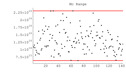
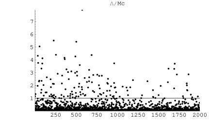
  Figure 3: The random samplings of the compactification scale $M_{c}$ and the ration $\Lambda/M_{c}$ for Pattern I. Level of fine-tuning: 7 $\%$. The physical solutions satisfy $\Lambda/M_{c}>1$.The range of the contributions from the SO(10)-breaking brane terms is $\delta_{i}^{(b)}\in\left[-2/\pi,+2/\pi\right]$. The horizontal lines in the first figure correspond to the maximum and the minimum values of $M_{c}$.

  Since we want to construct a predictive theory, it’s hopeful that the SO(10) symmetric contribution to the gauge coupling constants dominates over the SO(10) non-symmetric one. For this reason, the growth of $\delta^{(b)}_{i}$ leads a corresponding growth of $\Lambda R$ in order to keep under control the brane kinetic contribution. Nevertheless, as shown in the scatter plots Fig. 3, the numerical solutions have likely low values of $\Lambda/M_{c}$ ( $\Lambda/M_{c}<10$). Consequently the highly fine-tuned solutions are not acceptable anyway.

• Pattern II

  In the case with high VEV scales, Case A, there are numerical solutions even if we turn off the brane kinetic contributions $\delta_{i}^{(b)}$. The brane kinetic terms introduce a theoretical uncertainty on the determination of the compactification scale. We have used Eq.(27) to perform our numerical solutions of RGE and the Fig.4 and Fig.5 show the compactification scale $M_{c}$ and the ration $\Lambda/M_{c}$ versus SUSY spectrum for the Case A with 2 different values of $x$. The dominant errors come from the unknown SO(10) violating brane interactions parametrized by the random distribution $\delta_{i}^{(b)}\in(-1/2\pi,+1/2\pi)$. From the graphics of the ration $\Lambda/M_{c}$, we can see that the average value of $\Lambda/M_{c}$ for $x=1$ is about 1000 and it depends very sensitively on the parameter $x$.

  In the other regime, $\langle\Sigma\rangle\leq M_{c}$, that is Case B, the situation changes completely because $\delta^{(h)}_{s}<0$. We have shown numerically that this case is essentially similar to that of Pattern I and we will not reproduce the scatter plots for this case. For the most extreme regime where $\langle\Sigma\rangle\ll M_{c}$, we have already shown analytically in Sec. (3.2.2) that Pattern II is ruled out. Moving to $\langle\Sigma\rangle\approx M_{c}$, the numerical check shows that $\delta^{(h)}_{s}>-15/14\pi\log(\Lambda/M_{c})$ for low values of $\Lambda/M_{c}\lesssim 100$ but the sign is always negative, then the conclusion is unchanged. Then Case B is strongly disfavored for Pattern II.

  

  

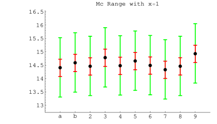
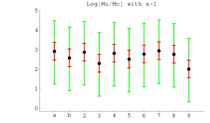
  Figure 4: Compactification scale $M_{c}$ and the ration $\Lambda/M_{c}$ versus SUSY spectrum for the Case A of the Pattern II with $x=1$. The shorter error bar represent the parametric error dominated by the experimental uncertainty on $\alpha_{3}(m_{Z})$, the wider bar includes the dominant source of error, the SO(10)-breaking brane terms $\delta_{i}^{(b)}\in\left[-1/2\pi,+1/2\pi\right]$.

  

  

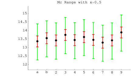
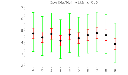
  Figure 5: Compactification scale $M_{c}$ and the ration $\Lambda/M_{c}$ versus SUSY spectrum for the Case A of the Pattern II with $x=1/2$. Error bars as in Fig. 4.

5 Conclusion

SUSY GUTs with extradimensions based on SO(10) gauge group, not only mantain the beautiful feature of unifying all matter including right handed neutrino in the same gauge multiplet, but also overcome some problems derived from the difficulty to explain the lightness of Higgs doublets and the heavyness of Higgs triplets, both occuring in the same gauge multiplet, without the introduction of a complicated or fine-tuned scalar sector, as happened in four-dimensional GUTs. The complete breaking of SO(10) gauge group, with rank equal to 5, to the SM gauge group, with rank 4, requires both orbifold and Higgs mechanisms. The latter can proceed in two different ways, but preferring one to another is not a trivial choice, as it has a great impact on the gauge coupling unification as we have showed in this paper.

Conventional four-dimensional SUSY GUTs predict in general a value of the strong coupling constant $\alpha_{3}(m_{z})$ higher than the largest value allowed by its experimental error. In 5D, it’s possible to improve the precision of the gauge coupling unification including the contribution derived from KK particles since this heavy threshold contribution could bring back $\alpha_{3}(m_{z})$ inside the experimental interval. The correct sign of heavy thresholds depends on the patterns used to break the SO(10) gauge symmetry to that of the SM. If we want to preserve the requirement of a precise natural unification, which is the inspiring principle of GUTs, we are inclined to prefer Higgs mechanism on the PS brane with a VEV near the cutoff scale, as it gives the desired prediction for the sign of the Kaluza Klein contributions, restoring the correct value for the $\alpha_{3}(m_{z})$ for a ration $\Lambda/M_{c}\gtrsim 100$.

We have then performed a detailed analysis of the gauge coupling unification for all possible models, in which the SO(10) gauge symmetry can be reduced to the Standard Model preserving the automatic D-T splitting, including all next-to-leading effects. We have provided also a numerical confirmation of our result. Our conclusion is that, as far as concerning the gauge coupling unification, Higgs mechanism on the PS brane is to be preferred to the one on the SO(10) preserving brane.

Acknowledgments We thank Ferruccio Feruglio for useful discussions and for his encouragement in our work. This project is partially supported by the European Program MRTN-CT-2004-503369.

References

- [1] R. Dermisek and A. Mafi, Phys. Rev. D 65 (2002) 055002.
- [2] H. D. Kim and S. Raby, JHEP 0301 (2003) 056.
- [3] Y. Nomura, D. R. Smith and N. Weiner, Nucl. Phys. B 613 (2001) 147.
- [4] M. L. Alciati, F. Feruglio, Y. Lin and A. Varagnolo, JHEP 0503 (2005) 054.
- [5] Y. Kawamura, Prog. Theor. Phys. 105 (2001) 999.
- [6] G. Altarelli and F. Feruglio, Phys. Lett. B 511 (2001) 257.
- [7] A. Hebecker and J. March-Russell, Nucl. Phys. B 613 (2001) 3.
- [8] A. Hebecker and J. March-Russell, Nucl. Phys. B 625 (2002) 128.
- [9] L. J. Hall and Y. Nomura, Phys. Rev. D 64 (2001) 055003.
- [10] Y. Nomura, Phys. Rev. D 65 (2002) 085036.
- [11] L. J. Hall and Y. Nomura, Phys. Rev. D 66 (2002) 075004.
- [12] S. P. Martin and P. Ramond, Phys. Rev. D 51, 6515 (1995); N. G. Deshpande, B. Dutta and E. Keith, Phys. Lett. B 384 (1996) 116.
- [13] R. Contino, L. Pilo, R. Rattazzi and E. Trincherini, Nucl. Phys. B 622 (2002) 227.
- [14] H. Georgi, A. K. Grant and G. Hailu, Phys. Lett. B 506 (2001) 207
- [15] J. Scherk and J. H. Schwarz, Phys. Lett. B 82 (1979) 60; J. Scherk and J. H. Schwarz, Nucl. Phys. B 153 (1979) 61.
- [16] P. Fayet, Phys. Lett. B 159 (1985) 121.
- [17] R. Barbieri, L. J. Hall and Y. Nomura, Phys. Rev. D 66 (2002) 045025; R. Barbieri, L. J. Hall and Y. Nomura, Nucl. Phys. B 624 (2002) 63.
- [18] L. J. Hall, H. Murayama and N. Weiner, Phys. Rev. Lett. 84 (2000) 2572; N. Haba and H. Murayama, Phys. Rev. D 63 (2001) 053010.
- [19] B. C. Allanach et al., in Proc. of the APS/DPF/DPB Summer Study on the Future of Particle Physics (Snowmass 2001) ed. N. Graf, Eur. Phys. J. C 25 (2002) 113.
- [20] See, for instance: G. Costa and F. Feruglio, Nuovo Cim. A 69 (1982) 195; G. Costa and F. Zwirner, Riv. Nuovo Cim. 9N3 (1986) 1.
- [21] S. Eidelman et al. [Particle Data Group Collaboration], Phys. Lett. B 592, 1 (2004).
- [22] D. R. T. Jones, Phys. Rev. D 25 (1982) 581; M. B. Einhorn and D. R. T. Jones, Nucl. Phys. B 196 (1982) 475.
- [23] See for instance: Y. Yamada, Z. Phys. C 60 (1993) 83.