Abstract

In this paper we describe the implementation of processes $f_{1}\bar{f}_{1}ZZ\to 0$ and $f_{1}\bar{f}_{1}HZ\to 0$ into the framework of SANC system. The $f_{1}$ stands for a massless fermion $f$ whose mass is kept non-zero only in arguments of $\ln$ functions and $\to 0$ means that all 4-momenta flow inwards. The derived scalar form factors can be used for any cross channel after an appropriate permutation of their arguments ($s,t,u$). We present the covariant and helicity amplitudes for these processes: for the former only in the annihilation channel $f_{1}\bar{f}_{1}\to ZZ$, while for the latter in annihilation $f_{1}\bar{f}_{1}\to HZ$ and decay $H\to Zf_{1}\bar{f}_{1}$ channels. We briefly describe additional precomputation modules which were not covered in the previous paper. For the processes $f_{1}\bar{f}_{1}\to HZ(ZZ)$ and decay $H\to Zf_{1}\bar{f}_{1}$ we present compact results of calculation of the accompanying bremsstrahlung and discuss exhaustive numerical results.

As applications there are two types of the Monte Carlo generators for the process $H\to 4\mu$. The first one is the generator based on a single resonance approximation for one of the $Z$ bosons. The second one, exploiting the double resonance approximation, is not described in this article. For the generator in the single approximation we present a short description.

Whenever possible, we compare our results with those existing in the literature. For example, we present a comparison of the results for $H\to 4\mu$ decay with those obtained by MC generator Prophecy4f.

SANC client for version v.1.10 can be downloaded from servers at CERN http://pcphsanc.cern.ch/ (137.138.39.23) and Dubna http://sanc.jinr.ru/ (159.93.75.10).

(Submitted to Computer Physics Communications)

^⋆ Supported in part by EU grant MTKD-CT-2004-510126, in the partnership with CERN PH/TH Division.
Supported in part by INTAS grant $N^{o}$ 03-51-4007.
^∗ Corresponding author.
^∗E-mail addresses: sanc@jinr.ru, bardindy@mail.cern.ch (D. Bardin)

1 Introduction

In this paper we continue to describe the computer system SANC Support of Analytic and Numerical Calculations for experiments at Colliders [1] intended for semi-automatic calculations of realistic and pseudo-observables for various processes of elementary particle interactions at the one-loop precision level. This is done in the spirit of the first description of the SANC system (see [1] and references therein which we recommend as a first acquaintance with the system).

Here we consider the implementation of several processes of $ffbb\to 0$ kind (where $f$ stands for a fermion, $b$ for a boson of the Standard Model (SM), while for concrete bosons we use $A$ for the photon and $Z,\;W^{\pm},\;H$) One should emphasize also that the notation $ffbb\to 0$ means that all external 4-momenta flow inwards; this is the standard SANC convention which allows to compute one-loop covariant amplitude (CA) and form factors (FF) only once and obtain it for a concrete channel by means of a crossing transformation. The present level of the system is realized in version v.1.10. Compared to version v.1.00, it is upgraded both physics-wise and computer-wise. As far as physics is concerned it contains an upgraded treatment of $u\bar{d}\to l^{+}\nu_{l}$ and $d\bar{u}\to l^{-}\bar{\nu}_{l}$ processes (see Ref. [2]) and a complete implementation of $F\to f+f_{1}+\bar{f^{{}^{\prime}}_{1}}$ CC decays up to numbers and MC generators. (Here $F$ and $f$ stand for massive fermions and $f_{1}$ and $\bar{f^{{}^{\prime}}_{1}}$ for massless fermions of the first generation.) Although the version 1.10 tree literally contains only $t\to b+l^{+}+\nu_{l}$ decay [3], any decay of the kind $F\to f+f_{1}+\bar{f^{{}^{\prime}}_{1}}$ may be treated in a similar manner and we are going to implement them into the next versions. The complete description of these CC decays will be given elsewhere [4]. Version 1.10 contains also the process $H\to f_{1}\bar{f}_{1}A$ in three cross channels [5] in EW branch, $\gamma\gamma\to\gamma\gamma$ scattering [6] and $l\,l\to\gamma\gamma^{*}$ in QED branch, as well as a new QCD branch [7].

New in version 1.10 are also several $ffbb\to 0$ processes, to whose implementation this paper is devoted. We describe here two of them: $f_{1}\bar{f}_{1}ZZ\to 0$ and $f_{1}\bar{f}_{1}HZ\to 0$, the latter one being used in two channels — annihilation and decay.

In the annihilation channel, these processes were considered in the literature extensively (see, for instance, [8] and [9]–[10]), however, we are not aware of publications devoted to the $H\to Zf_{1}\bar{f}_{1}$ decay.

These processes are relevant for $H$ search at LHC: the processes $f_{1}\bar{f}_{1}\to ZZ$ are one of the backgrounds while the one-loop calculations of the decay $H\to Zf_{1}\bar{f}_{1}$ was also used for an improved treatment of the decay $H\to 4\mu$ for an intermediate Higgs mass interval 130 GeV $\leq M_{\scriptscriptstyle{H}}\leq$ 150 GeV, see section 7.

Furthermore, in the spirit of the adopted SANC approach, all $2f2b\to 0$ processes can be computed with off shell bosons thereby allowing their use also as building blocks for future studies of $5\to 0$ processes.

The process $f_{1}\bar{f}_{1}ZZ$ is very similar to the processes $ffb\gamma$ ($b=\gamma,\,Z\,,H$) whose precomputation was described in detail in Ref. [1]. Its tree level amplitude is represented by two diagrams in $t$ and $u$ channels, Fig. 1.

$$\begin{array}[]{ccc}\vbox{\hbox{ \begin{picture}(132.0,132.0)(0.0,0.0) \put(0.0,0.0){} \put(0.0,0.0){} \put(0.0,0.0){} \put(0.0,0.0){} \put(0.0,0.0){} \put(0.0,0.0){} \put(0.0,0.0){} \put(0.0,0.0){} \put(0.0,0.0){} \put(0.0,0.0){} \put(0.0,0.0){} \raise 132.0pt\hbox to0.0pt{\kern-32.0pt\makebox(0.0,0.0)[lt]{\sf ii}\hss} \ignorespaces \raise 118.0pt\hbox to0.0pt{\kern 42.0pt\makebox(0.0,0.0)[lb]{$p_{4}$}\hss} \ignorespaces \raise 5.0pt\hbox to0.0pt{\kern 42.0pt\makebox(0.0,0.0)[lb]{$p_{3}$}\hss} \ignorespaces \raise 60.0pt\hbox to0.0pt{\kern 42.0pt\makebox(0.0,0.0)[lb]{$t$-channel}\hss} \ignorespaces \raise 106.0pt\hbox to0.0pt{\kern-15.0pt\makebox(0.0,0.0)[lb]{$\nu$}\hss} \ignorespaces \raise 105.0pt\hbox to0.0pt{\kern 60.0pt\makebox(0.0,0.0)[lb]{vu=typeFU}\hss} \ignorespaces \raise 18.0pt\hbox to0.0pt{\kern 60.0pt\makebox(0.0,0.0)[lb]{vd=typeFD}\hss} \ignorespaces \raise 137.0pt\hbox to0.0pt{\kern-42.0pt\makebox(0.0,0.0)[lb]{fu=typeIU}\hss} \ignorespaces \raise-12.0pt\hbox to0.0pt{\kern-42.0pt\makebox(0.0,0.0)[lb]{fd=typeID}\hss} \ignorespaces \raise 17.0pt\hbox to0.0pt{\kern-15.0pt\makebox(0.0,0.0)[lb]{$\mu$}\hss} \ignorespaces \raise 123.0pt\hbox to0.0pt{\kern-4.0pt\makebox(0.0,0.0)[lb]{$p_{1}$}\hss} \ignorespaces \raise 3.0pt\hbox to0.0pt{\kern-4.0pt\makebox(0.0,0.0)[lb]{$p_{2}$}\hss} \ignorespaces \raise-13.0pt\hbox to0.0pt{\kern 35.0pt\makebox(0.0,0.0)[lb]{a)}\hss} \ignorespaces \end{picture}}}&&\vbox{\hbox{ \begin{picture}(132.0,132.0)(0.0,0.0) \put(0.0,0.0){} \put(0.0,0.0){} \put(0.0,0.0){} \put(0.0,0.0){} \put(0.0,0.0){} \put(0.0,0.0){} \put(0.0,0.0){} \put(0.0,0.0){} \put(0.0,0.0){} \put(0.0,0.0){} \put(0.0,0.0){} \raise 132.0pt\hbox to0.0pt{\kern-32.0pt\makebox(0.0,0.0)[lt]{\sf ii}\hss} \ignorespaces \raise 118.0pt\hbox to0.0pt{\kern 42.0pt\makebox(0.0,0.0)[lb]{$p_{3}$}\hss} \ignorespaces \raise 5.0pt\hbox to0.0pt{\kern 42.0pt\makebox(0.0,0.0)[lb]{$p_{4}$}\hss} \ignorespaces \raise 60.0pt\hbox to0.0pt{\kern 42.0pt\makebox(0.0,0.0)[lb]{$u$-channel}\hss} \ignorespaces \raise 106.0pt\hbox to0.0pt{\kern-15.0pt\makebox(0.0,0.0)[lb]{$\nu$}\hss} \ignorespaces \raise 105.0pt\hbox to0.0pt{\kern 60.0pt\makebox(0.0,0.0)[lb]{vd=typeFD}\hss} \ignorespaces \raise 18.0pt\hbox to0.0pt{\kern 60.0pt\makebox(0.0,0.0)[lb]{vu=typeFU}\hss} \ignorespaces \raise 137.0pt\hbox to0.0pt{\kern-42.0pt\makebox(0.0,0.0)[lb]{fu=typeIU}\hss} \ignorespaces \raise-12.0pt\hbox to0.0pt{\kern-42.0pt\makebox(0.0,0.0)[lb]{fd=typeID}\hss} \ignorespaces \raise 17.0pt\hbox to0.0pt{\kern-15.0pt\makebox(0.0,0.0)[lb]{$\mu$}\hss} \ignorespaces \raise 123.0pt\hbox to0.0pt{\kern-4.0pt\makebox(0.0,0.0)[lb]{$p_{1}$}\hss} \ignorespaces \raise 3.0pt\hbox to0.0pt{\kern-4.0pt\makebox(0.0,0.0)[lb]{$p_{2}$}\hss} \ignorespaces \raise-13.0pt\hbox to0.0pt{\kern 35.0pt\makebox(0.0,0.0)[lb]{b)}\hss} \ignorespaces \end{picture}}}\end{array}$$

Figure 1: Born $ffHZ(ZZ)\to 0$ diagrams, $t$ and $u$ channels.

Figure 2: Born $ffHZ\to 0$ diagrams, $s$ channel.

Note, that in this and in the following figures, fu=typeIU etc. denote “types” of external particles, see Table 2 of [1] as well as the discussion in the beginning of section 4.

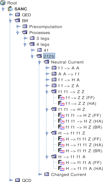
Figure 3: New processes in the EW part.

For the process $f_{1}\bar{f}_{1}\to HZ$ these two diagrams do not contribute in the tree approximation since fermion $f_{1}$ is considered to be massless. However, in this case there exists an $s$ channel amplitude, Fig. 2,

All $ffbb$ processes are fully implemented at Level 1 of analytical calculations. Several new modules which compute the contribution of the $bbb$ vertices to $ffbb\to 0$ processes are added to the precomputation tree, as well as three other modules relevant for the $s$ channel diagram.

The modified “Precomputation” tree is shown in Fig. 5 and discussed in section 3.

The modified branch 2f2b for the “Processes” tree is shown in Fig. 3. It contains four new sub-menus $f_{1}\bar{f}_{1}\to ZZ$, $f_{1}\bar{f}_{1}\to HZ$, $H\to f_{1}\bar{f}_{1}Z$ and $H\to f_{1}\bar{f}_{1}A$ which in turn are branched into scalar Form Factors (FF) and Helicity Amplitudes (HA) (two for the process $f_{1}\bar{f}_{1}HZ$ corresponding to two annihilation and decay channels) and the accompanying bremsstrahlung contributions (BR).

These processes are implemented also at Level 2, where the s2n.f package produces the results in the “Semi Analytic” mode (see Fig. 20 of Ref. [1]). For the three decays we have relevant “Monte Carlo” generators which, however, are not yet implemented into the system.

The paper is organized as follows:

In section 2 we describe the covariant (CA) and helicity amplitudes for three of four new $ffbb\to 0$ processes available in version 1.10.

Section 3 contains a brief description of new precomputation modules. In section 4 we describe in some more detail the renormalization procedure for the $f_{1}\bar{f}_{1}HZ\to 0$ process, i.e. calculation of FFs. Section 5 contains the results for the accompanying bremsstrahlung in the semi-analytic mode for two $f_{1}\bar{f}_{1}HZ\to 0$ channels. Section 6 contains numerical results for the processes $f_{1}\bar{f}_{1}\to HZ(ZZ)$ and decay $H\to Zf_{1}\bar{f}_{1}$. Finally, section 7 contains a brief description a Monte Carlo generator for process $H\to 4\mu$ in the single resonance approximation. The first results of numerical comparison with those of Prophecy4f [11]–[12] are also presented.

2 Amplitude Basis, Scalar Form Factors, Helicity Amplitudes

2.1 Introduction

In this section we continue the presentation of formulae for the amplitudes of $ffbb\to 0$ processes started in section 2 of Ref. [1]. As usual, we begin with the calculation of CAs corresponding to a result of the straightforward computation of all diagrams contributing to a given process at the one-loop level. It is represented in a certain basis of structures, made of strings of Dirac matrices and external momenta, contracted with polarization vectors of vector bosons. The amplitude is parameterized by a number of FFs, which we denote by ${\cal F}$ with an index labeling the corresponding structure. The number of FFs is by construction equal to the number of structures, however for the cases presented below some of the FFs can be equal, so the number of independent FFs may be less than the number of structures. For the existing tree level structures the corresponding FFs have the form

$${\cal F}=1+\frac{\alpha}{4\pi s_{\scriptscriptstyle{W}}^{2}}{\tilde{\cal F}}\,,$$ (1)

where “1” is due to the Born level and ${\tilde{\cal F}}$ is due to the one-loop level. As usual, we use various coupling constants:

$$Q_{f}\,,\quad I^{(3)}_{f}\,,\quad\sigma_{f}=v_{f}+a_{f}\,,\quad\delta_{f}=v_{f}-a_{f}\,,\quad s_{\scriptscriptstyle{W}}=\frac{e}{g}\,,\quad c_{\scriptscriptstyle{W}}=\frac{M_{\scriptscriptstyle{W}}}{M_{\scriptscriptstyle{Z}}}\,,\quad\mbox{\it etc.}$$ (2)

Given a CA, SANC computes a set of HAs, denoted by ${\cal H}_{\lambda_{1}\lambda_{2}\lambda_{3}\dots}$, where $\lambda_{1}\lambda_{2}\lambda_{3}\dots$ denote the signs of particle spin projections onto a quantization axis.

2.2 $f\bar{f}\to ZZ$ process

Here we present the CA of the process $f(p_{2})\bar{f}(p_{1})\to Z(p_{3})Z(p_{4})$ in the annihilation channel , see Fig. 1.

It contains 10 left $(\gamma_{+})$ and 10 right $(\gamma_{-})$ structures:

$${\cal A}_{\scriptscriptstyle{f}fZZ} = k_{0}\,\Biggl{\{}\Biggl{[}{\bar{v}}\left({p_{1}}\right)\biggl{(}/\!\!\!p_{3}\gamma_{+}(p_{1})_{\mu}(p_{1})_{\nu}{\cal F}^{+}_{1}(s,t)+/\!\!\!p_{3}\gamma_{+}(p_{1})_{\mu}(p_{2})_{\nu}{\cal F}^{+}_{2}(s,t)$$ (3)

$$\phantom{-\frac{i}{8c_{\scriptscriptstyle{W}}^{2}}\,\Biggl{\{}\Biggl{[}}+/\!\!\!p_{3}\gamma_{+}(p_{1})_{\nu}(p_{2})_{\mu}{\cal F}^{+}_{3}(s,t)+/\!\!\!p_{3}\gamma_{+}(p_{2})_{\mu}(p_{2})_{\nu}{\cal F}^{+}_{4}(s,t)+/\!\!\!p_{3}\gamma_{+}\delta_{\mu\nu}{\cal F}^{+}_{5}(s,t)$$

$$\phantom{-\frac{i}{8c_{\scriptscriptstyle{W}}^{2}}\,\Biggl{\{}\Biggl{[}}+\gamma_{\mu}/\!\!\!p_{3}\gamma_{\nu}\gamma_{+}{\cal F}^{+}_{6}(s,t)+\gamma_{\mu}\gamma_{+}(p_{1})_{\nu}{\cal F}^{+}_{7}(s,t)+\gamma_{\mu}\gamma_{+}(p_{2})_{\nu}{\cal F}^{+}_{8}(s,t)$$

$$\phantom{-\frac{i}{8c_{\scriptscriptstyle{W}}^{2}}\,\Biggl{\{}\Biggl{[}}+\gamma_{\nu}\gamma_{+}(p_{1})_{\mu}{\cal F}^{+}_{9}(s,t)+\gamma_{\nu}\gamma_{+}(p_{2})_{\mu}{\cal F}^{+}_{10}(s,t)\biggr{)}u\left({p_{2}}\right)\varepsilon^{\scriptscriptstyle{Z}}_{\nu}(p_{3})\varepsilon^{\scriptscriptstyle{Z}}_{\mu}(p_{4})\Biggr{]}$$

$$\phantom{-\frac{i}{8c_{\scriptscriptstyle{W}}^{2}}\,\Biggl{\{}\Biggl{[}}+\Biggl{[}\gamma_{+}\to\gamma_{-},\,{\cal F}^{+}_{i}\to{\cal F}^{-}_{i}\Biggr{]}\Biggr{\}},$$

where

$$k_{0}=-\frac{ig^{2}}{8c_{\scriptscriptstyle{W}}^{2}}\qquad\mbox{and}\qquad\gamma_{\pm}=I\pm\gamma_{5}\,.$$ (4)

Furthermore,

$$\left(p_{1}+p_{2}\right)^{2}=-s,\qquad\left(p_{2}+p_{3}\right)^{2}=-t,\qquad\left(p_{2}+p_{4}\right)^{2}=-u.$$ (5)

Now we give the explicit form of the CA in the tree (Born) approximation:

$${\cal A}^{\scriptscriptstyle{B}orn}_{\scriptscriptstyle{f}fZZ} = k_{0}\,\Biggl{\{}\Biggl{[}\sigma_{f}^{2}{\bar{v}}\left({p_{1}}\right)\Biggl{(}\frac{t+u}{tu}\,\gamma_{\mu}/\!\!\!p_{3}\gamma_{\nu}\gamma_{+}+\frac{2}{t}\,\gamma_{\mu}\gamma_{+}(p_{2})_{\nu}\ +\frac{2}{u}\,\biggl{(}/\!\!\!p_{3}\gamma_{+}\delta_{\mu\nu}$$ (6)

$$-\gamma_{\mu}\gamma_{+}(p_{1})_{\nu}+\gamma_{\nu}\gamma_{+}(p_{1})_{\mu}+\gamma_{\nu}\gamma_{+}(p_{2})_{\mu}\biggr{)}\Biggr{)}u\left({p_{2}}\right)\varepsilon^{\scriptscriptstyle{Z}}_{\nu}(p_{3})\varepsilon^{\scriptscriptstyle{Z}}_{\mu}(p_{4})\Biggr{]}$$

$$+\Biggl{[}\sigma_{f}^{2}\to\delta_{f}^{2},\;\gamma_{+}\to\gamma_{-}\Biggr{]}\Biggr{\}}.$$

Note that this is decomposed into 12 structures of 20 and is highly asymmetric in $t$ and $u$. This is due to our choice of the 4-momentum $p_{3}$ and of the ordering of Lorentz indices $\mu$ and $\nu$ in Eq. (6).

Equation 6 may be parameterized by only two FFs if one introduces two “Born-like structures (BLS)” given by expressions in big round brackets by means of eliminating the 5th structure $/\!\!\!p_{3}\gamma_{+}\delta_{\mu\nu}$ in favor of BLS; to this structure and to the corresponding ${\cal F}^{\pm}_{0}(s,t)$ we assign the subindex “0”:

$$/\!\!\!p_{3}\gamma_{\pm}\delta_{\mu\nu} = -\frac{u}{2}\Bigg{[}{\mbox{\rm BLS}}^{\pm}_{0}+\left(\frac{1}{t}+\frac{1}{u}\right)\gamma_{\mu}/\!\!\!p_{3}\gamma_{\nu}\gamma_{\pm}\Bigg{]}-\frac{u}{t}\gamma_{\mu}\gamma_{\pm}(p_{2})_{\nu}+\gamma_{\mu}\gamma_{\pm}(p_{1})_{\nu}-\gamma_{\nu}\gamma_{\pm}(p_{1})_{\mu}+\gamma_{\nu}\gamma_{\pm}(p_{2})_{\mu}\;.$$ (7)

Moreover, between the 20 FFs there are four identities:

$${\cal F}^{\pm}_{4}(s,t)={\cal F}^{\pm}_{1}(s,t),\quad{\cal F}^{\pm}_{10}(s,t)=-{\cal F}^{\pm}_{7}(s,t).$$ (8)

Therefore, there are 16 independent FFs but 18 independent non-zero HAs for process $f_{1}\bar{f}_{1}\to ZZ$:

$${\cal H}_{+-\pm\mp} = k^{s}_{0}c_{\pm}\biggl{\{}\mp 2\sigma_{e}^{2}\left(\frac{1}{t}+\frac{1}{u}\right){\cal F}^{+}_{0}(s,t)+\frac{s}{4}c_{\mp}\beta\left[2{\cal F}^{+}_{1}(s,t)-{\cal F}^{+}_{2}(s,t)-{\cal F}^{+}_{3}(s,t)\right]$$

$$\mp 2{\cal F}^{+}_{7}(s,t)\pm{\cal F}^{+}_{8}(s,t)\mp{\cal F}^{+}_{9}(s,t)\biggr{\}},$$

$${\cal H}_{-+\pm\mp} = k^{s}_{0}c_{\mp}\biggl{\{}\mp 2\delta_{e}^{2}\left(\frac{1}{t}+\frac{1}{u}\right){\cal F}^{-}_{0}(s,t)-\frac{s}{4}c_{\pm}\beta\left[2{\cal F}^{-}_{1}(s,t)-{\cal F}^{-}_{2}(s,t)-{\cal F}^{-}_{3}(s,t)\right]$$

$$\mp 2{\cal F}^{-}_{7}(s,t)\pm{\cal F}^{-}_{8}(s,t)\mp{\cal F}^{-}_{9}(s,t)\biggr{\}},$$

$${\cal H}_{+-\pm\pm} = k^{s}_{0}\biggl{\{}-2\sigma_{e}^{2}\left(\frac{\beta^{c}_{-}}{t}-\frac{\beta^{c}_{+}}{u}\right){\cal F}^{+}_{0}(s,t)-\frac{s}{4}\sin^{2}{\vartheta_{\scriptscriptstyle{Z}}}\beta\left[2{\cal F}^{+}_{1}(s,t)-{\cal F}^{+}_{2}(s,t)-{\cal F}^{+}_{3}(s,t)\right]$$

$$+2\left[\beta_{\mp}{\cal F}^{+}_{6}(s,t)+\cos{{\vartheta}_{\scriptscriptstyle{Z}}}{\cal F}^{+}_{7}(s,t)\right]\pm c_{\mp}{\cal F}^{+}_{8}(s,t)\pm c_{\pm}{\cal F}^{+}_{9}(s,t)\biggr{\}},$$

$${\cal H}_{-+\mp\mp} = k^{s}_{0}\biggl{\{}2\delta_{e}^{2}\left(\frac{\beta^{c}_{-}}{t}-\frac{\beta^{c}_{+}}{u}\right){\cal F}^{-}_{0}(s,t)+\frac{s}{4}\sin^{2}{{\vartheta}_{\scriptscriptstyle{Z}}}\beta\left[2{\cal F}^{-}_{1}(s,t)-{\cal F}^{-}_{2}(s,t)-{\cal F}^{-}_{3}(s,t)\right]$$

$$-2\left[\beta_{\mp}{\cal F}^{-}_{6}(s,t)+\cos{{\vartheta}_{\scriptscriptstyle{Z}}}{\cal F}^{-}_{7}(s,t)\right]\mp\frac{1}{2}c_{\mp}{\cal F}^{-}_{8}(s,t)\mp\frac{1}{2}c_{\pm}{\cal F}^{-}_{9}(s,t)\biggr{\}},$$

$${\cal H}_{+-\pm 0} = k_{1}^{\pm}\biggl{\{}2\sigma_{el}^{2}\left[\frac{\beta^{c}_{-}}{t}-\frac{\beta^{c}_{+}}{u}\pm\frac{2M_{\scriptscriptstyle{Z}}^{2}}{s}\left(\frac{1}{t}+\frac{1}{u}\right)\right]{\cal F}^{+}_{0}(s,t)$$

$$-\frac{s}{4}c_{\mp}\beta\left[\mp 2\cos{{\vartheta}_{\scriptscriptstyle{Z}}}{\cal F}^{+}_{1}(s,t)\mp\beta^{c}_{-}{\cal F}^{+}_{2}(s,t)\pm\beta^{c}_{+}{\cal F}^{+}_{3}(s,t)\right]$$

$$\pm\beta_{-}^{2}{\cal F}^{+}_{6}(s,t)-\left(\beta^{c}_{+}\mp c_{\mp}\right){\cal F}^{+}_{7}(s,t)\mp c_{\mp}{\cal F}^{+}_{8}(s,t)+\beta^{c}_{-}{\cal F}^{+}_{9}(s,t)\biggr{\}},$$

$${\cal H}_{+-0\pm} = k_{1}^{\mp}\biggl{\{}2\sigma_{e}^{2}\left[\frac{\beta^{c}_{-}}{t}-\frac{\beta^{c}_{+}}{u}\mp\frac{2M_{\scriptscriptstyle{Z}}^{2}}{s}\left(\frac{1}{t}+\frac{1}{u}\right)\right]{\cal F}^{+}_{0}(s,t)$$

$$-\frac{s}{4}c_{\pm}\beta\left[\pm 2\cos{{\vartheta}_{\scriptscriptstyle{Z}}}{\cal F}^{+}_{1}(s,t)\pm\beta^{c}_{-}{\cal F}^{+}_{2}(s,t)\mp\beta^{c}_{+}{\cal F}^{+}_{3}(s,t)\right]$$

$$\pm 4\frac{M_{\scriptscriptstyle{Z}}^{2}}{s}{\cal F}^{+}_{6}(s,t)-\left(\beta^{c}_{+}\pm c_{\pm}\right){\cal F}^{+}_{7}(s,t)-\beta^{c}_{-}{\cal F}^{+}_{8}(s,t)\mp c_{\pm}{\cal F}^{+}_{9}(s,t)\biggr{\}},$$

$${\cal H}_{-+\pm 0} = k_{1}^{\mp}\biggl{\{}2\delta_{el}^{2}\left[\frac{\beta^{c}_{-}}{t}-\frac{\beta^{c}_{+}}{u}\mp\frac{2M_{\scriptscriptstyle{Z}}^{2}}{s}\left(\frac{1}{t}+\frac{1}{u}\right)\right]{\cal F}^{-}_{0}(s,t)$$

$$+\frac{s}{4}c_{\pm}\beta\left[\mp 2\cos{{\vartheta}_{\scriptscriptstyle{Z}}}{\cal F}^{-}_{1}(s,t)\mp\beta^{c}_{-}{\cal F}^{-}_{2}(s,t)\pm\beta^{c}_{+}{\cal F}^{-}_{3}(s,t)\right]$$

$$\mp\beta_{+}^{2}{\cal F}^{-}_{6}(s,t)-\left(\beta^{c}_{+}\pm c_{\pm}\right){\cal F}^{-}_{7}(s,t)\pm c_{\pm}{\cal F}^{-}_{8}(s,t)+\beta^{c}_{-}{\cal F}^{-}_{9}(s,t)\biggr{\}},$$

$${\cal H}_{-+0\pm} = k_{1}^{\pm}\biggl{\{}2\delta_{el}^{2}\left[\frac{\beta^{c}_{-}}{t}-\frac{\beta^{c}_{+}}{u}\pm\frac{2M_{\scriptscriptstyle{Z}}^{2}}{s}\left(\frac{1}{t}+\frac{1}{u}\right)\right]{\cal F}^{-}_{0}(s,t)$$

$$\pm\frac{s}{4}c_{\mp}\beta\Bigl{(}2\cos{{\vartheta}_{\scriptscriptstyle{Z}}}{\cal F}^{-}_{1}(s,t)+\beta^{c}_{-}{\cal F}^{-}_{2}(s,t)-\beta^{c}_{+}{\cal F}^{-}_{3}(s,t)\Bigr{)}$$

$$\mp 4\frac{M_{\scriptscriptstyle{Z}}^{2}}{s}{\cal F}^{-}_{6}(s,t)-\left(\beta^{c}_{+}\mp c_{\mp}\right){\cal F}^{-}_{7}(s,t)-\beta^{c}_{-}{\cal F}^{-}_{8}(s,t)\pm c_{\mp}{\cal F}^{-}_{9}(s,t)\biggr{\}},$$

$${\cal H}_{\pm\mp 00} = \frac{k^{s}_{0}}{2}\frac{s}{M_{\scriptscriptstyle{Z}}^{2}}\biggl{\{}\mp 2\left(\begin{array}[]{c}\sigma_{el}^{2}\\ \delta_{el}^{2}\end{array}\right)\left[\frac{\beta^{c}_{-}}{t}-\frac{\beta^{c}_{+}}{u}+2\beta_{f}\frac{M_{\scriptscriptstyle{Z}}^{2}}{s}\left(\frac{1}{t}-\frac{1}{u}\right)\right]{\cal F}^{\pm}_{0}(s,t)$$ (12)

$$\mp\frac{1}{4}s\beta\left[2\beta^{c}_{+}\beta^{c}_{-}{\cal F}^{\pm}_{1}(s,t)+(\beta^{c}_{-})^{2}{\cal F}^{\pm}_{2}(s,t)+(\beta^{c}_{+})^{2}{\cal F}^{\pm}_{3}(s,t)\right]$$

$$+4\beta\frac{M_{\scriptscriptstyle{Z}}^{2}}{s}{\cal F}^{\pm}_{6}(s,t)\pm 2\beta^{c}_{+}{\cal F}^{\pm}_{7}(s,t)\pm\beta^{c}_{-}\left[{\cal F}^{\pm}_{8}(s,t)-{\cal F}^{\pm}_{9}(s,t)\right]\biggr{\}}.$$

Here we use the following shorthand notation:

$$k^{s}_{0} = \frac{k_{0}s}{2}\sin{\vartheta}_{\scriptscriptstyle{Z}},\quad k^{\pm}_{1}=\frac{k_{0}s}{2}\frac{\sqrt{s}}{\sqrt{2}M_{\scriptscriptstyle{Z}}}c_{\pm}\,,\quad c_{\pm}=1\pm\cos{\vartheta}_{\scriptscriptstyle{Z}},\qquad$$

$$\beta_{\pm} = \beta\pm 1,\qquad\quad\beta^{c}_{\pm}=\beta\pm\cos{\vartheta}_{\scriptscriptstyle{Z}},\qquad\beta=\frac{\sqrt{\lambda(s,M_{\scriptscriptstyle{Z}}^{2},M_{\scriptscriptstyle{Z}}^{2})}}{s}\,,$$ (13)

and $\vartheta_{\scriptscriptstyle{Z}}$ is the CMS angle between $\vec{p}_{2}$ and $\vec{p}_{3}$. The invariant $t$ and the cosine $\cos{\vartheta}_{\scriptscriptstyle{Z}}$ are related by

$$t=M_{\scriptscriptstyle{Z}}^{2}-\frac{1}{2}s(1-\beta\cos{\vartheta}_{\scriptscriptstyle{Z}})\,.$$ (14)

The number 18 is the product of 2 initial massless helicity states and 3$\times$3 states for the final $Z$ bosons.

2.3 $f_{1}\bar{f}_{1}\to HZ$ process

There are six structures for the $f_{1}\bar{f}_{1}\to HZ$ process if the fermion mass is neglected

$${\cal A}_{\scriptscriptstyle{ffHZ}} = k\,\Biggl{\{}\Biggl{[}{\bar{v}}\left({p_{1}}\right)\biggl{(}\gamma_{\nu}\gamma_{+}\sigma_{f}{\cal F}^{+}_{0}(s,t)+/\!\!\!p_{3}\gamma_{+}(p_{1})_{\nu}{\cal F}^{+}_{1}(s,t)+/\!\!\!p_{3}\gamma_{+}(p_{2})_{\nu}{\cal F}^{+}_{2}(s,t)\biggr{)}u\left({p_{2}}\right)\varepsilon^{\scriptscriptstyle{Z}}_{\nu}(p_{3})\Biggr{]}$$ (15)

$$\phantom{-\frac{ig^{2}}{8c_{\scriptscriptstyle{W}}^{2}}}+\Biggl{[}\sigma_{f}\to\delta_{f},\;\gamma_{+}\to\gamma_{-},\;{\cal F}^{+}_{i}(s,t)\to{\cal F}^{-}_{i}(s,t)\Biggr{]}\Biggr{\}},$$

where

$$k=-\frac{ig^{2}}{4c_{\scriptscriptstyle{W}}^{2}}\frac{M_{\scriptscriptstyle{Z}}}{M_{\scriptscriptstyle{Z}}^{2}-s}\,.$$ (16)

The structures for the decay $H\to f_{1}\bar{f}_{1}Z$ may be obtained by simple replacement of 4-momenta $p_{1}\to-p_{3},\,p_{2}\to-p_{4},\,p_{4}\to-p_{1}\,(p_{3}\to p_{2})$ of the structures (15).

Note, that the two terms $\gamma_{\nu}\gamma_{+}\sigma_{f}{\cal F}^{\pm}_{0}(s,t)$ correspond to the Born level.

As far as HAs are concerned, we present them in both channels: annihilation and decay.

2.3.1 HAs in annihilation channel $f_{1}\bar{f}_{1}\to HZ$

There are 6 HAs in this case:

$${\cal H}_{+-+} = \phantom{+}k^{s}_{0}c_{+}\Bigl{\{}k^{-}_{1}\left[{\cal F}^{+}_{2}(s,t)-{\cal F}^{+}_{1}(s,t)\right]-4\sigma_{e}{\cal F}^{+}_{0}(s,t)\Bigr{\}},$$

$${\cal H}_{-++} = -k^{s}_{0}c_{-}\Bigl{\{}k^{+}_{1}\left[{\cal F}^{-}_{1}(s,t)-{\cal F}^{-}_{2}(s,t)\right]+4\delta_{e}{\cal F}^{-}_{0}(s,t)\Bigr{\}},$$

$${\cal H}_{+--} = -k^{s}_{0}c_{-}\Bigl{\{}k^{+}_{1}\left[{\cal F}^{+}_{1}(s,t)-{\cal F}^{+}_{2}(s,t)\right]+4\sigma_{e}{\cal F}^{+}_{0}(s,t)\Bigr{\}},$$

$${\cal H}_{-+-} = \phantom{+}k^{s}_{0}c_{+}\Bigl{\{}k^{-}_{1}\left[{\cal F}^{-}_{2}(s,t)-{\cal F}^{-}_{1}(s,t)\right]-4\delta_{e}{\cal F}^{-}_{0}(s,t)\Bigr{\}},$$

$${\cal H}_{+-0} = \phantom{+}k^{s}_{0}k_{2}\Bigl{\{}{\sqrt{\lambda(s,M_{\scriptscriptstyle{Z}}^{2},M_{\scriptscriptstyle{H}}^{2})}}\left[\beta^{c}_{+}{\cal F}^{+}_{1}(s,t)+\beta^{c}_{-}{\cal F}^{+}_{2}(s,t)\right]+4\sigma_{e}{\cal F}^{+}_{0}(s,t)\Bigr{\}},$$

$${\cal H}_{-+0} = -k^{s}_{0}k_{2}\Bigl{\{}{\sqrt{\lambda(s,M_{\scriptscriptstyle{Z}}^{2},M_{\scriptscriptstyle{H}}^{2})}}\left[\beta^{c}_{+}{\cal F}^{-}_{1}(s,t)+\beta^{c}_{-}{\cal F}^{-}_{2}(s,t)\right]+4\delta_{e}{\cal F}^{-}_{0}(s,t)\Bigr{\}}.$$ (17)

where

$$k^{s}_{0} = k_{0}\frac{1}{\sqrt{2}}\frac{\sqrt{s}M_{\scriptscriptstyle{Z}}}{s-M_{\scriptscriptstyle{Z}}^{2}}\,,\qquad k^{\pm}_{1}=\sqrt{\lambda(s,M_{\scriptscriptstyle{Z}}^{2},M_{\scriptscriptstyle{H}}^{2})}c_{\pm}\,,\qquad k_{2}=\frac{s+M_{\scriptscriptstyle{Z}}^{2}-M_{\scriptscriptstyle{H}}^{2}}{\sqrt{2}\sqrt{s}M_{\scriptscriptstyle{Z}}}\sin{\vartheta_{\scriptscriptstyle{Z}}},$$

$$c_{\pm} = 1\pm\cos{\vartheta_{\scriptscriptstyle{Z}}},\qquad\beta^{c}_{\pm}=\beta\pm\cos{\vartheta_{\scriptscriptstyle{Z}}},\qquad\beta=\frac{\sqrt{\lambda(s,M_{\scriptscriptstyle{Z}}^{2},M_{\scriptscriptstyle{H}}^{2})}}{s+M_{\scriptscriptstyle{Z}}^{2}-M_{\scriptscriptstyle{H}}^{2}}\,,$$

$$t = M_{\scriptscriptstyle{Z}}^{2}-\frac{1}{2}(s+M_{\scriptscriptstyle{Z}}^{2}-M_{\scriptscriptstyle{H}}^{2})(1-\beta\cos{\vartheta_{\scriptscriptstyle{Z}}})\,.$$ (18)

2.3.2 HAs in the decay channel $H\to f_{1}\bar{f}_{1}Z$

The six HAs in this case are somewhat different from the previous case:

$${\cal H}_{++-} = k^{s}_{0}\Bigl{\{}k_{1}\left[{\cal F}^{-}_{1}(s,t)-{\cal F}^{-}_{2}(s,t)\right]-4\delta_{f}c_{-}{\cal F}^{-}_{0}(s,t)\Bigr{\}},$$

$${\cal H}_{+-+} = k^{s}_{0}\Bigl{\{}k_{1}\left[{\cal F}^{+}_{2}(s,t)-{\cal F}^{+}_{1}(s,t)\right]-4\sigma_{f}c_{+}{\cal F}^{+}_{0}(s,t)\Bigr{\}},$$

$${\cal H}_{-+-} = k^{s}_{0}\Bigl{\{}k_{1}\left[{\cal F}^{-}_{1}(s,t)-{\cal F}^{-}_{2}(s,t)\right]+4\delta_{f}c_{+}{\cal F}^{-}_{0}(s,t)\Bigr{\}},$$

$${\cal H}_{--+} = k^{s}_{0}\Bigl{\{}k_{1}\left[{\cal F}^{+}_{2}(s,t)-{\cal F}^{+}_{1}(s,t)\right]+4\sigma_{f}c_{-}{\cal F}^{+}_{0}(s,t)\Bigr{\}},$$

$${\cal H}_{0+-} = k^{s}_{0}k_{2}\Bigl{\{}\phantom{-}\sqrt{\lambda{(M_{\scriptscriptstyle{H}}^{2},M_{\scriptscriptstyle{Z}}^{2},s)}}\left[\beta^{c}_{+}{\cal F}^{-}_{1}(s,t)+\beta^{c}_{-}{\cal F}^{-}_{2}(s,t)\right]-4\delta_{e}{\cal F}^{-}_{0}(s,t)\Bigr{\}},$$

$${\cal H}_{0-+} = k^{s}_{0}k_{2}\Bigl{\{}-\sqrt{\lambda(M_{\scriptscriptstyle{H}}^{2},M_{\scriptscriptstyle{Z}}^{2},s)}\left[\beta^{c}_{+}{\cal F}^{+}_{1}(s,t)+\beta^{c}_{-}{\cal F}^{+}_{2}(s,t)\right]+4\sigma_{e}{\cal F}^{+}_{0}(s,t)\Bigr{\}}.$$ (19)

Here,

$$k^{s}_{0} = k_{0}\frac{1}{\sqrt{2}}\frac{\sqrt{s}M_{\scriptscriptstyle{Z}}}{M_{\scriptscriptstyle{Z}}^{2}-s}\,,\qquad k_{1}=\sqrt{\lambda(M_{\scriptscriptstyle{H}}^{2},M_{\scriptscriptstyle{Z}}^{2},s)}\sin^{2}{\vartheta_{f}},\qquad k_{2}=\frac{\left(M_{\scriptscriptstyle{H}}^{2}-M_{\scriptscriptstyle{Z}}^{2}-s\right)}{\sqrt{2}\sqrt{s}M_{\scriptscriptstyle{Z}}}\sin{\vartheta_{f}},$$

$$c_{\pm} = 1\pm\cos{\vartheta_{f}},\qquad\beta^{c}_{\pm}=\beta\pm\cos{\vartheta_{f}},\qquad\beta=\frac{\sqrt{\lambda(M_{\scriptscriptstyle{H}}^{2},M_{\scriptscriptstyle{Z}}^{2},s)}}{M_{\scriptscriptstyle{H}}^{2}-M_{\scriptscriptstyle{Z}}^{2}-s}\,.$$ (20)

The number 6 is the product of 2 initial massless helicity states and 3 states of the final $Z$ boson.

Furthermore, $s=M^{2}_{f_{1}\bar{f}_{1}}$ is the invariant mass of the two fermions $f$, varying in the limits $4m^{2}_{f}\leq s\leq(M_{\scriptscriptstyle{H}}-M_{\scriptscriptstyle{Z}})^{2}$; and $t$ is another independent kinematical variable, depending on $s$ and an angle $\vartheta_{f}$, varying in the limits $0\leq\vartheta_{f}\leq\pi$

$$t=M_{\scriptscriptstyle{Z}}^{2}+\frac{1}{2}\left[M_{\scriptscriptstyle{H}}^{2}-M_{\scriptscriptstyle{Z}}^{2}-s-\sqrt{\lambda(M_{\scriptscriptstyle{H}}^{2},M_{\scriptscriptstyle{Z}}^{2},s)}\cos{\vartheta_{f}}\right].$$ (21)

The kinematical diagram of the process is shown in Fig. 4.

Figure 4: $H\to f_{1}\bar{f}_{1}Z$ decay kinematics.

The Higgs boson with momentum $p_{2}$ at rest, decays back-to-back into a $Z$ boson with momentum $p_{1}$ and a fermionic compound with 4-momentum $p_{3}+p_{4}$ and invariant mass $s$. This compound decays in its own rest frame into two back-to-back fermions with $\vartheta_{f}$ being the angle between $p_{3}$ in the compound rest frame and the direction of flight of the $Z$ boson in the $H$ boson rest frame.

3 Precomputation news

The “Precomputation” tree of version 1.10 is shown in Fig. 5 with all modified sub-menus open, and all sub-menus closed which were not changed compared to version 1.00. In this section we briefly discuss what every new module does.

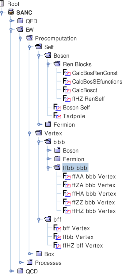
Figure 5: New EW precomputation modules.

First, we added a new folder accessible via menu sequence EW $\to$ Precomputation $\to$ Vertex $\to$ bbb $\to$ ffbb bbb with five modules ffXX bbb Vertex, XX=AA, ZA, HA, ZZ, HZ which compute three boson vertices of four topologies (see Fig. 11 of Ref. [1]) to the corresponding $ffbb$ processes, Fig. 6. The results of their calculations are saved to ffXX*.sav files to be loaded by corresponding modules computing FFs via chains EW $\to$ Processes $\to$ 4-legs $\to$ 2f2b $\to$ Neutral Current for the $ffXX\to 0$ processes.

These three boson diagrams contain both bosonic and fermionic components. The latter are precomputed by the modules bbb Vertex in Boson and Fermion folders of the same level on the tree. Five modules of ffbb bbb folder load them and then apply tedious calculations involving in some cases the Schouten identity. There are many peculiarities in these calculations, forcing us to have an individual module for each $ffbb$ process. Note also that if the corresponding process has a Born-level $s$ channel exchange as in Fig. 2, then the contribution of one-loop vertices is supplemented by the relevant counterterm cross.

In the modules under discussion a summation over the exchanged boson $B$ is performed. In general, four neutral bosons $B=\gamma,Z,\phi^{0}$ and $H$ can contribute if the fermion mass is not neglected, otherwise, only $\gamma$ and $Z$ contribute.

For the processes $ffAA\to 0$, $ffZA\to 0$, $ffHA\to 0$ the “left” $bff$ vertex diagram, shown in Fig. 7 does not contribute, since in these cases the “right” vertex does not exist at the tree level. In general, and this is indeed the case for the processes $ffZZ\to 0$ and $ffHZ\to 0$, the “right” vertex exists at the tree level for $B=Z,\phi^{0}$, therefore, the dressed “left” vertex has to be added to the precomputation tree. Note that it does not contribute for massless fermions if $B=\phi^{0}$. For $ffHZ\to 0$ this vertex is accessible via menu sequence EW $\to$ Precomputation $\to$ Vertex $\to$ bff $\to$ ffHZ bff Vertex. For the $ffZZ\to 0$ process, only $B=H$ contributes, but then, for the massless $f$, the dressed “left” vertex vanishes. This is why we do not add the corresponding module in the latter case.

Figure 6: “Right” $bbb$ vertex in $ffbb$ processes.

Figure 7: “Left” $bff$ vertex in $ffbb$ processes.

The presence of an $s$ channel tree level diagram in the process $f_{1}\bar{f}_{1}HZ\to 0$ (Fig. 2) forces us to take into account two more self energy diagrams, Fig. 8.

$$\begin{array}[]{cc}\begin{picture}(125.0,86.0)(0.0,0.0) \put(0.0,0.0){} \put(0.0,0.0){} \put(0.0,0.0){} \put(0.0,0.0){} \put(0.0,0.0){} \put(0.0,0.0){} \put(0.0,0.0){} \put(0.0,0.0){} \raise 90.0pt\hbox to0.0pt{\kern-15.0pt\makebox(0.0,0.0)[lb]{fd=typeID}\hss} \ignorespaces \raise-13.0pt\hbox to0.0pt{\kern-15.0pt\makebox(0.0,0.0)[lb]{fu=typeIU}\hss} \ignorespaces \raise 90.0pt\hbox to0.0pt{\kern 110.0pt\makebox(0.0,0.0)[lb]{vu=typeFU}\hss} \ignorespaces \raise-13.0pt\hbox to0.0pt{\kern 110.0pt\makebox(0.0,0.0)[lb]{vd=typeFD}\hss} \ignorespaces \par \put(0.0,0.0){} \put(0.0,0.0){} \par \raise 48.0pt\hbox to0.0pt{\kern 35.0pt\makebox(0.0,0.0)[cb]{$B_{1}$}\hss} \ignorespaces \raise 48.0pt\hbox to0.0pt{\kern 90.0pt\makebox(0.0,0.0)[cb]{$B_{2}$}\hss} \ignorespaces \raise 76.0pt\hbox to0.0pt{\kern 11.0pt\makebox(0.0,0.0)[lb]{$p_{1}$}\hss} \ignorespaces \raise 3.0pt\hbox to0.0pt{\kern 10.0pt\makebox(0.0,0.0)[lb]{$p_{2}$}\hss} \ignorespaces \raise 76.0pt\hbox to0.0pt{\kern 127.0pt\makebox(0.0,0.0)[lb]{$H$}\hss} \ignorespaces \raise 3.0pt\hbox to0.0pt{\kern 127.0pt\makebox(0.0,0.0)[lb]{$Z$}\hss} \ignorespaces \put(0.0,0.0){} \put(0.0,0.0){} \par \raise 76.0pt\hbox to0.0pt{\kern 105.0pt\makebox(0.0,0.0)[lb]{$p_{4}$}\hss} \ignorespaces \raise 3.0pt\hbox to0.0pt{\kern 104.0pt\makebox(0.0,0.0)[lb]{$p_{3}$}\hss} \ignorespaces \par\end{picture}&\qquad\qquad\qquad\begin{picture}(125.0,86.0)(0.0,0.0) \put(0.0,0.0){} \put(0.0,0.0){} \put(0.0,0.0){} \put(0.0,0.0){} \put(0.0,0.0){} \put(0.0,0.0){} \put(0.0,0.0){} \put(0.0,0.0){} \put(0.0,0.0){} \raise 90.0pt\hbox to0.0pt{\kern-15.0pt\makebox(0.0,0.0)[lb]{fd=typeID}\hss} \ignorespaces \raise-13.0pt\hbox to0.0pt{\kern-15.0pt\makebox(0.0,0.0)[lb]{fu=typeIU}\hss} \ignorespaces \raise 90.0pt\hbox to0.0pt{\kern 110.0pt\makebox(0.0,0.0)[lb]{vu=typeFU}\hss} \ignorespaces \raise-13.0pt\hbox to0.0pt{\kern 110.0pt\makebox(0.0,0.0)[lb]{vd=typeFD}\hss} \ignorespaces \par \put(0.0,0.0){} \put(0.0,0.0){} \par \raise 48.0pt\hbox to0.0pt{\kern 62.5pt\makebox(0.0,0.0)[cb]{$Z$}\hss} \ignorespaces \raise 48.0pt\hbox to0.0pt{\kern 127.0pt\makebox(0.0,0.0)[lb]{$H$}\hss} \ignorespaces \raise 76.0pt\hbox to0.0pt{\kern 11.0pt\makebox(0.0,0.0)[lb]{$p_{1}$}\hss} \ignorespaces \raise 3.0pt\hbox to0.0pt{\kern 10.0pt\makebox(0.0,0.0)[lb]{$p_{2}$}\hss} \ignorespaces \raise 76.0pt\hbox to0.0pt{\kern 127.0pt\makebox(0.0,0.0)[lb]{$H$}\hss} \ignorespaces \raise 3.0pt\hbox to0.0pt{\kern 127.0pt\makebox(0.0,0.0)[lb]{$Z$}\hss} \ignorespaces \par \put(0.0,0.0){} \put(0.0,0.0){} \par \raise 76.0pt\hbox to0.0pt{\kern 105.0pt\makebox(0.0,0.0)[lb]{$p_{4}$}\hss} \ignorespaces \raise 3.0pt\hbox to0.0pt{\kern 104.0pt\makebox(0.0,0.0)[lb]{$p_{3}$}\hss} \ignorespaces \par\end{picture}\end{array}$$

Figure 8: Self energy $ffHZ$ diagrams.

The first one is accessible via menu chain: Self $\to$ Boson $\to$ Ren Blocks $\to$ ffHZ Ren Self. Here $B_{1}=\gamma,Z,\phi^{0}$ and $B_{2}=Z,\phi^{0}$; again $\phi^{0}$’s do not contribute for massless fermions. As will be explained in the next section, the second diagram is better to be combined with the “right” vertex, Fig. 6.

Note that nothing is changed, compared to $ffXA$ processes, as far as boxes are concerned. So, the Box sub-menu is as in version 1.00 [1].

The new modules contain calls to several new intrinsic procedures which will be described elsewhere.

4 Renormalizaton for $ffHZ\to 0$ process

In this section we describe how to use the FORM [13] module which computes FFs for the process $ffHZ\to 0$. This description is supposed to help a user to understand the other modules computing FFs for any $ffbb\to 0$ process.

First of all, to use our basic declaration and notation we begin the file with

#include Declar.h
#call Globals()

and define types of external particles, see Figs. 1 and 2.

#ifdef ‘typeIU’;  *  ‘fu’
#ifdef ‘typeID’;  *  ‘fd’
#ifdef ‘typeFU’;  *  ‘vu’
#ifdef ‘typeFD’;  *  ‘vd’
#define typeIDp "{2*(‘typeID’%2)-1+‘typeID’}";  * ‘fdp’

Secondly, we fix four main steering flags to define the calculation Al scheme:

1. define xi: xi = 0 to test gauge invariance in $R_{\xi}$, or xi = 1 to work in $\xi=1$ gauge;

2. define on: on = 0 external photons are off mass-shell, or on = 1 photons are on mass-shell;

3. define mf: mf = 0 zero external fermion mass (i.e. pm(‘fd’)=0), or mf = 1 it is not zeroed;

4. define mp: mp = 0 zero mass of the weak isospin partner of the fermion $f$, pm(‘fdp’)=0, or mp = 1 it is not zeroed.

Actually, for the process under consideration, $f_{1}\bar{f}_{1}HZ\to 0$, only the $\xi$ and mp definitions are meaningful since there are no external photons and we ignore the masses of external fermions throughout the calculations. But the mass of a weak isospin partner of an external fermion that appears in the internal loop may be kept nonzero.

The ideology of building blocks (BB) is the key element for SANC development. The information about the main precomputed BB is stored in basic *.sav files (BSF). Note that for 4-particle $ffbb$ processes all the BBs are 4-legs by construction. This trick will greatly simplify the procedure of projection of the covariant amplitude onto an independent basis of structures.

Moreover, for the future development it is necessary to upgrade the database of the collected information area SANC: fields of program modules, fields of procedures and the bank of BSF.

Any module computing FFs starts from loading of the calculated BB from the bank of BSF. These BSF contain the precomputed objects: self energies, vertices and boxes typically with off-shell bosons.

They are precomputed not only to accelerate the calculations. Although all BSF may be, in principle, precomputed online, we remind that in some cases the CPU time for calculating off-shell boxes in $R_{\xi}$ gauge takes many hours, see section 3.4 of Ref. [1]. In such cases precomputation is strictly prohibited and the user must use already precomputed BSFs.

We recall also that our precomputation procedure has indeed several levels; in the modules computing FFs we tend to use the results of the last level which contains already renormalized BBs: propagators and vertices, i.e. taking into account relevant counterterms and special vertices, [14]. However, they are full of residual UV poles and $\xi$ dependent terms, which cancel in the sum for a one-loop CA of a physical process. This is why we still use to word “renormalization” in connection with modules computing FFs rather than a simple “summation”.

Typically, the loading of BSFs is organized in several steps. Let us consider the example of H $\to$ f1 f1 Z (FF) module, see the tree in Fig. 5.

• step self

  Here we manipulate objects from BSF ffHZSelfschxi‘xi’‘fu’‘fd’‘vu’‘vd’.sav

  We extract from its volume the BB of bosonic self energy in the s-channel, BSEsch‘fu’‘fd’‘vu’‘vd’ see left diagram in Fig. 8.

• step vertex

  Moving further over the renormalization procedure at this step we load three BSFs:
  ffHZVertbffxi‘xi’‘fu’‘fd’‘vu’‘vd’.sav;
  ffHZVertbbbxi‘xi’‘fu’‘fd’‘vu’‘vd’.sav;
  ffbbVertxi‘xi’on‘on’mf‘mf’mp‘mp’‘fu’‘fd’‘vu’‘vd’.sav.

  From these BSFs we extract various types of vertices correspondingly:
  — VertBff‘i’‘fu’‘fd’‘vu’‘vd’ with i=1,2,3,4 standing for $\xi_{\scriptscriptstyle{A}}$, $\xi_{\scriptscriptstyle{Z}}$, $\xi_{\scriptscriptstyle{W}}$, and no $\xi$ vertex clusters originating from the diagram of Fig. 7;
  — Vertbbbbos‘fu’‘fd’‘vu’‘vd’ and Vertbbbfer‘fu’‘fd’‘vu’‘vd’ — the bosonic and fermionic components of three-boson vertices shown in the diagram Fig. 6, where the former contains counterterms, the special vertex and the right diagram of Fig. 8. These tadpoles cancel the $\xi_{\scriptscriptstyle{Z}}$ dependence of the three-boson vertices, giving an opportunity to assign this contribution to i=3. Finally, the fermionic component should be naturally assigned to i=4;
  — abelian Vert‘I’‘i’ and non-abelian vert‘I’‘i’ vertex clusters in $t$ and $u$ channels I=t,u with cluster index i=1,2,3,4 and k=22,33,24,42,44, see section 3.4.2 of Ref. [1] for a description of the latter.

• step boxes

  Here the most complex building blocks — off-shell boxes are loaded from four BSFs:
  ffbb3T1xi‘xi’on‘on’mf‘mf’mp‘mp’‘fu’‘fd’‘vd’‘vu’.sav;
  ffbb3T3xi‘xi’on‘on’mf‘mf’mp‘mp’‘fu’‘fd’‘vu’‘vd’.sav;
  ffbb22T5xi‘xi’on‘on’mf‘mf’mp‘mp’‘vd’‘fd’‘vu’‘fu’.sav;
  ffbb33T5xi‘xi’on‘on’mf‘mf’mp‘mp’‘vd’‘fd’‘vu’‘fu’.sav.

  They contain precomputed boxes of topology T1 from the expression S3T1‘xi’‘on’‘mf’‘mp’‘fu’‘fd’ ‘vd’‘vu’, the boxes of topology T3 from the expression S3T3‘xi’‘on’‘mf’‘mp’‘fu’‘fd’‘vu’‘vd’, and of topology T5 with cluster index $k1=2,3$ , i.e. with virtual $Z$ and $W$ bosons from the expression S‘k1’‘k1’T5‘xi’‘on’‘mf’‘mp’‘vd’‘fd’‘vu’‘fu’, see section 3.4.2 of Ref. [1].

  Only those box topologies and clusters are loaded which give a non-zero contribution for $m_{f}=0$.

• step Sum

  Finally, we sum all contributions. Four expressions, Sum‘i’, corresponding to cluster index i=1,2,3,4 are being constructed here. The first three of them may carry only one gauge parameter each, the latter carries none.

After construction of four Sum‘i’, the module continues with various kinds of transformations (in particular, involving an algebra of Gram determinants) which prove the cancellation of gauge parameter dependences in first three Sum1,2,3 and the cancellation of the residual UV poles between FFs with cluster indices i=3 and i=4.

After the comment Preparing Structures for obtaining FFs: the six basis elements of the CA, Eq (15), are created and the 6$\times 4$ FFs are projected out of this CA.

The final step is formatting of the BSF FFf1f1HZ.sav with $24$ FFs --- FFgp‘k’‘i’ and FFgm‘k’‘i’ ($k=0,1,2$, $i=1,4$) --- for subsequent processing by s2n.f software.

5 Bremsstrahlung in $f_{1}\bar{f}_{1}HZ\to 0$ processes

In this section we present the list of short final results for the contribution of accompanying bremsstrahlung processes.

5.1 Bremsstrahlung in $f_{1}\bar{f}_{1}\to HZ$ annihilation channel

The tree level diagram of this channel is shown in Fig. 2. The corresponding total Born cross section reads:

$$\sigma^{\rm Born}=\frac{G_{\scriptscriptstyle{F}}^{2}(v_{f}^{2}+a_{f}^{2})}{12\pi}\frac{M_{\scriptscriptstyle{Z}}^{4}\sqrt{\lambda\big{(}s,M_{\scriptscriptstyle{Z}}^{2},M_{\scriptscriptstyle{H}}^{2}\big{)}}}{(M_{\scriptscriptstyle{Z}}^{2}-s)^{2}+M_{\scriptscriptstyle{Z}}^{2}\Gamma^{2}_{\scriptscriptstyle{Z}}}\left[\frac{1}{2}+\frac{1}{s}\left(5M_{\scriptscriptstyle{Z}}^{2}-M_{\scriptscriptstyle{H}}^{2}\right)+\frac{1}{2s^{2}}\left(M_{\scriptscriptstyle{H}}^{2}-M_{\scriptscriptstyle{Z}}^{2}\right)^{2}\right].$$ (22)

There are only two initial state (ISR) bremsstrahlung diagrams:

$$\begin{array}[]{cc}\begin{picture}(125.0,86.0)(0.0,0.0) \put(0.0,0.0){} \put(0.0,0.0){} \put(0.0,0.0){} \put(0.0,0.0){} \put(0.0,0.0){} \put(0.0,0.0){} \put(0.0,0.0){} \put(0.0,0.0){} \put(0.0,0.0){} \raise 76.0pt\hbox to0.0pt{\kern 11.0pt\makebox(0.0,0.0)[lb]{$p_{1}$}\hss} \ignorespaces \raise 3.0pt\hbox to0.0pt{\kern 10.0pt\makebox(0.0,0.0)[lb]{$p_{2}$}\hss} \ignorespaces \raise 66.0pt\hbox to0.0pt{\kern 40.0pt\makebox(0.0,0.0)[cb]{$p_{5}$}\hss} \ignorespaces \put(0.0,0.0){} \put(0.0,0.0){} \raise 76.0pt\hbox to0.0pt{\kern 127.0pt\makebox(0.0,0.0)[lb]{$H$}\hss} \ignorespaces \put(0.0,0.0){} \raise 76.0pt\hbox to0.0pt{\kern 105.0pt\makebox(0.0,0.0)[lb]{$p_{4}$}\hss} \ignorespaces \raise 3.0pt\hbox to0.0pt{\kern 127.0pt\makebox(0.0,0.0)[lb]{$Z$}\hss} \ignorespaces \put(0.0,0.0){} \raise 3.0pt\hbox to0.0pt{\kern 104.0pt\makebox(0.0,0.0)[lb]{$p_{3}$}\hss} \ignorespaces \end{picture}&\qquad\qquad\begin{picture}(125.0,86.0)(0.0,0.0) \put(0.0,0.0){} \put(0.0,0.0){} \put(0.0,0.0){} \put(0.0,0.0){} \put(0.0,0.0){} \put(0.0,0.0){} \put(0.0,0.0){} \put(0.0,0.0){} \put(0.0,0.0){} \raise 76.0pt\hbox to0.0pt{\kern 11.0pt\makebox(0.0,0.0)[lb]{$p_{1}$}\hss} \ignorespaces \raise 3.0pt\hbox to0.0pt{\kern 10.0pt\makebox(0.0,0.0)[lb]{$p_{2}$}\hss} \ignorespaces \raise 18.0pt\hbox to0.0pt{\kern 40.0pt\makebox(0.0,0.0)[ct]{$p_{5}$}\hss} \ignorespaces \put(0.0,0.0){} \put(0.0,0.0){} \raise 76.0pt\hbox to0.0pt{\kern 127.0pt\makebox(0.0,0.0)[lb]{$H$}\hss} \ignorespaces \put(0.0,0.0){} \raise 76.0pt\hbox to0.0pt{\kern 105.0pt\makebox(0.0,0.0)[lb]{$p_{4}$}\hss} \ignorespaces \raise 3.0pt\hbox to0.0pt{\kern 127.0pt\makebox(0.0,0.0)[lb]{$Z$}\hss} \ignorespaces \put(0.0,0.0){} \raise 3.0pt\hbox to0.0pt{\kern 104.0pt\makebox(0.0,0.0)[lb]{$p_{3}$}\hss} \ignorespaces \par\end{picture}\end{array}$$

Figure 9: Bremsstrahlung diagrams in annihilation channel

QED corrections due to virtual and soft photons are proportional to the Born cross section:

$$\sigma^{\rm Virt}={\sigma^{\rm Born}}\frac{\alpha}{\pi}Q_{f}^{2}\left\{\frac{1}{2}\left[\ln\left(\frac{s}{m_{f}^{2}}\right)-1\right]^{2}+\left[\frac{3}{2}-\ln\left(\frac{s}{\lambda^{2}}\right)\right]\left[\ln\left(\frac{s}{m_{f}^{2}}\right)-1\right]-1+4\mbox{${\rm{Li}}_{2}$}(1)\right\},$$ (23)

$$\sigma^{\rm Soft}={\sigma^{\rm Born}}\frac{\alpha}{\pi}Q_{f}^{2}\left\{-\frac{1}{2}\left[\ln\left(\frac{s}{m_{f}^{2}}\right)-1\right]^{2}+\ln\left(\frac{4\bar{\omega}^{2}}{\lambda^{2}}\right)\left[\ln\left(\frac{s}{m_{f}^{2}}\right)-1\right]+\frac{1}{2}-2\mbox{${\rm{Li}}_{2}$}(1)\right\},$$ (24)

with infrared divergence $\ln{\lambda^{2}}$ being canceled out. The hard photon contribution of the differential cross section in $s^{\prime}=-(p_{3}+p_{4})^{2}$ has the following factorization property:

$$\frac{d\sigma^{\rm Hard}}{ds^{\prime}}=\frac{\alpha}{\pi}Q_{f}^{2}\frac{s^{2}+{s^{\prime}}^{2}}{s^{2}(s-s^{\prime})}\left[\ln\left(\frac{s}{m_{f}^{2}}\right)-1\right]\sigma^{\rm Born}(s^{\prime})\,.$$ (25)

It may be integrated over $s^{\prime}$ leading to a rather compact expression for $\sigma^{\rm{tot}}$ (see relevant module at SANC tree), yielding a $\ln{\bar{\omega}}$ which cancels against corresponding term in Eq. (24).

5.2 Bremsstrahlung in $H\to f_{1}\bar{f}_{1}Z$ decay channel

Here we consider the decay channel $H\to f_{1}\bar{f}_{1}Z$. We begin with the tree level diagram, Fig. 10:

$$\begin{array}[]{cc}\begin{picture}(132.0,132.0)(0.0,0.0) \put(0.0,0.0){} \put(0.0,0.0){} \raise 70.0pt\hbox to0.0pt{\kern 12.0pt\makebox(0.0,0.0)[lb]{$H$}\hss} \ignorespaces \put(0.0,0.0){} \put(0.0,0.0){} \put(0.0,0.0){} \raise 90.0pt\hbox to0.0pt{\kern 50.0pt\makebox(0.0,0.0)[lb]{$Z$}\hss} \ignorespaces \put(0.0,0.0){} \put(0.0,0.0){} \raise 37.0pt\hbox to0.0pt{\kern 115.0pt\makebox(0.0,0.0)[lb]{$\bar{f}_{1}$}\hss} \ignorespaces \raise-10.0pt\hbox to0.0pt{\kern 115.0pt\makebox(0.0,0.0)[lb]{$f_{1}$}\hss} \ignorespaces \raise 30.0pt\hbox to0.0pt{\kern 50.0pt\makebox(0.0,0.0)[lb]{$Z$}\hss} \ignorespaces \end{picture}\end{array}$$

Figure 10: The $H\to f_{1}\bar{f}_{1}Z$ decay tree level diagram.

The corresponding tree level double differential width, depending on two kinematical variables $s,\;\vartheta_{f}$ discussed in section 2.3.2 and with kinematics shown in Fig. 4, reads

$$\frac{d^{2}\Gamma^{\rm Born}}{ds\,d\cos\vartheta_{f}} = k_{\scriptscriptstyle{B}}\Biggl{\{}\Biggl{(}\left(v_{f}^{2}+a_{f}^{2}\right)\left[\sin^{2}\theta_{f}\left(1-4\frac{m_{f}^{2}}{s}\right)+4\frac{m_{f}^{2}}{s}\right]-8a_{f}^{2}\frac{m_{f}^{2}}{M_{\scriptscriptstyle{Z}}^{2}}\Biggr{)}$$ (26)

$$\left[\left(1-\frac{s}{M_{\scriptscriptstyle{H}}^{2}}\right)^{2}-2\frac{sM_{\scriptscriptstyle{Z}}^{2}}{M_{\scriptscriptstyle{H}}^{4}}-1+\left(1-\frac{M_{\scriptscriptstyle{Z}}^{2}}{M_{\scriptscriptstyle{H}}^{2}}\right)^{2}\right]+8\left(v_{f}^{2}+a_{f}^{2}\right)\frac{sM_{\scriptscriptstyle{Z}}^{2}}{M_{\scriptscriptstyle{H}}^{4}}\left(1+2\frac{m_{f}^{2}}{s}\right)$$

$$+4a_{f}^{2}\frac{m_{f}^{2}}{M_{\scriptscriptstyle{Z}}^{2}}\left[\frac{sM_{\scriptscriptstyle{Z}}^{2}}{M_{\scriptscriptstyle{H}}^{4}}\left(1-\frac{s}{M_{\scriptscriptstyle{Z}}^{2}}\right)^{2}+\frac{s}{M_{\scriptscriptstyle{H}}^{2}}\left(-2\frac{s}{M_{\scriptscriptstyle{Z}}^{2}}-2+\frac{M_{\scriptscriptstyle{H}}^{2}}{M_{\scriptscriptstyle{Z}}^{2}}\right)-12\frac{M_{\scriptscriptstyle{Z}}^{4}}{M_{\scriptscriptstyle{H}}^{4}}\right]\Biggr{\}},$$

$$\mbox{where}\hskip 11.38109ptk_{\scriptscriptstyle{B}}=\frac{1}{128}\frac{G^{2}_{\scriptscriptstyle{F}}}{\pi^{3}}\frac{\sqrt{\lambda\big{(}M_{\scriptscriptstyle{H}}^{2},M_{\scriptscriptstyle{Z}}^{2},s\big{)}}M_{\scriptscriptstyle{Z}}^{4}M_{\scriptscriptstyle{H}}}{\left|M_{\scriptscriptstyle{Z}}^{2}-iM_{\scriptscriptstyle{Z}}\Gamma_{\scriptscriptstyle{Z}}-s\right|^{2}}\,.$$

There are only two final state bremsstrahlung diagrams, Fig. 11:

$$\begin{array}[]{cc}\begin{picture}(132.0,132.0)(0.0,-25.0){ \put(0.0,0.0){} \put(0.0,0.0){} \raise 70.0pt\hbox to0.0pt{\kern 12.0pt\makebox(0.0,0.0)[lb]{$H$}\hss} \ignorespaces \put(0.0,0.0){} \put(0.0,0.0){} \put(0.0,0.0){} \raise 90.0pt\hbox to0.0pt{\kern 50.0pt\makebox(0.0,0.0)[lb]{$Z$}\hss} \ignorespaces \put(0.0,0.0){} \put(0.0,0.0){} \put(0.0,0.0){} \raise 62.0pt\hbox to0.0pt{\kern 135.0pt\makebox(0.0,0.0)[lb]{$\bar{f}_{1}$}\hss} \ignorespaces \raise-28.0pt\hbox to0.0pt{\kern 135.0pt\makebox(0.0,0.0)[lb]{$f_{1}$}\hss} \ignorespaces \raise 30.0pt\hbox to0.0pt{\kern 45.0pt\makebox(0.0,0.0)[lb]{$Z,\gamma$}\hss} \ignorespaces \put(0.0,0.0){} \raise 41.0pt\hbox to0.0pt{\kern 137.0pt\makebox(0.0,0.0)[lb]{$\gamma$}\hss} \ignorespaces } \end{picture}&\qquad\qquad\begin{picture}(132.0,132.0)(0.0,-25.0){ \put(0.0,0.0){} \put(0.0,0.0){} \raise 70.0pt\hbox to0.0pt{\kern 12.0pt\makebox(0.0,0.0)[lb]{$H$}\hss} \ignorespaces \put(0.0,0.0){} \put(0.0,0.0){} \put(0.0,0.0){} \raise 90.0pt\hbox to0.0pt{\kern 50.0pt\makebox(0.0,0.0)[lb]{$Z$}\hss} \ignorespaces \put(0.0,0.0){} \put(0.0,0.0){} \put(0.0,0.0){} \raise 62.0pt\hbox to0.0pt{\kern 135.0pt\makebox(0.0,0.0)[lb]{$\bar{f}_{1}$}\hss} \ignorespaces \raise-28.0pt\hbox to0.0pt{\kern 135.0pt\makebox(0.0,0.0)[lb]{$f_{1}$}\hss} \ignorespaces \raise 30.0pt\hbox to0.0pt{\kern 45.0pt\makebox(0.0,0.0)[lb]{$Z,\gamma$}\hss} \ignorespaces \put(0.0,0.0){} \raise-3.0pt\hbox to0.0pt{\kern 137.0pt\makebox(0.0,0.0)[lb]{$\gamma$}\hss} \ignorespaces } \end{picture}\end{array}$$

Figure 11: The $H\to f_{1}\bar{f}_{1}Z$ decay, bremsstrahlung.

The fully differential phase space is characterized by five kinematical variables which we choose as follows:

$$d\Phi^{(3)}=\frac{ds}{2\pi}\frac{d\tau}{2\pi}\,\Phi^{(2)}_{1}\,d\Phi^{(2)}_{2}\,d\Phi^{(2)}_{3}\,,$$ (27)

where $\tau=-(p_{4}+p_{5})^{2}$ is the lepton--photon invariant mass.

The 3-step kinematical cascade develops as a sequence of three 2-body decays shown in Fig. 12,

Figure 12: Bremsstrahlung kinematics.

with three corresponding two body phase spaces:

$$\Phi^{(2)}_{1} = \frac{1}{8\pi}\frac{\sqrt{\lambda\big{(}M_{\scriptscriptstyle{H}}^{2},M_{\scriptscriptstyle{Z}}^{2},s\big{)}}}{s}\,,$$

$$d\Phi^{(2)}_{2} = \frac{1}{8\pi}\frac{\sqrt{\lambda\big{(}s,\tau,m^{2}_{f}\big{)}}}{s}\,\frac{1}{2}\,d\cos\vartheta_{3}\,,$$

$$d\Phi^{(2)}_{3} = \frac{1}{8\pi}\frac{\sqrt{\lambda\big{(}\tau,m^{2}_{f},0\big{)}}}{\tau}\,\frac{1}{2}\,d\cos\vartheta_{4}\,\frac{1}{2\pi}d\varphi_{4}\,.$$ (28)

The gauge invariant QED part of the complete one-loop EW correction is subdivided into virtual, soft and hard photon contributions. The virtual one comes from the two Born-like FFs with cluster index i=1. It is proportional to the Born width and contains the infrared divergence parameterized by the photon mass $\lambda$:

$$\frac{d^{2}\Gamma^{\rm Virt}}{ds\,d\cos\vartheta_{f}}=\frac{d^{2}\Gamma^{\rm Born}}{ds\,d\cos\vartheta_{f}}\frac{\alpha}{\pi}Q_{f}^{2}\Biggl{\{}-\ln\left(\frac{m_{f}^{2}}{\lambda^{2}}\right)\left[\ln\left(\frac{s}{m_{f}^{2}}\right)-1\right]+\frac{1}{2}\ln\left(\frac{s}{m_{f}^{2}}\right)\left[3-\ln\left(\frac{s}{m_{f}^{2}}\right)\right]+4\mbox{${\rm{Li}}_{2}$}(1)-2\Biggl{\}}.$$ (29)

The soft photon contribution is also proportional to the Born one; its infrared divergence cancels against the virtual contribution. It contains also a logarithm with soft-hard separator $\bar{\omega}$:

$$\frac{d^{2}\Gamma^{\rm Soft}}{ds\,d\cos\vartheta_{f}}=\frac{d^{2}\Gamma^{\rm Born}}{ds\,d\cos\vartheta_{f}}\frac{\alpha}{\pi}Q_{f}^{2}\Biggl{\{}\left[\ln\left(\frac{m_{f}^{2}}{\lambda^{2}}\right)+2\ln\left(\frac{2\bar{\omega}}{m_{f}}\right)-\ln\left(\frac{s}{m_{f}^{2}}\right)\right]\left[\ln\left(\frac{s}{m_{f}^{2}}\right)-1\right]-\mbox{${\rm{Li}}_{2}$}\left(1\right)+1\Biggr{\}}.$$ (30)

The hard photon contribution after integration over three kinematical variables $d\varphi_{4}\,,\;d\cos\vartheta_{4}$ and $d\tau$ (the first two vary together in full angular $4\pi$ limits and $m^{2}_{f}\leq\tau\leq(\sqrt{s}-m_{f})^{2}$) is

$$\frac{d^{2}\Gamma^{\rm Hard}}{ds\,d\cos\vartheta_{f}} = \frac{d^{2}\Gamma^{\rm Born}}{ds\,d\cos\vartheta_{f}}\frac{\alpha}{\pi}Q_{f}^{2}\Biggl{\{}-2\ln\left(\frac{2\bar{\omega}}{m_{f}}\right)\left[\ln\left(\frac{s}{m_{f}^{2}}\right)-1\right]-\frac{1}{2}\ln\left(\frac{s}{m_{f}^{2}}\right)\left[5-3\ln\left(\frac{s}{m_{f}^{2}}\right)\right]$$ (31)

$$\hskip 25.60747pt-3\mbox{${\rm{Li}}_{2}$}(1)+\frac{1}{4}\Biggr{\}}+k_{\scriptscriptstyle{B}}\frac{\alpha}{\pi}Q_{f}^{2}\left[\left(1-\frac{s}{M_{\scriptscriptstyle{H}}^{2}}\right)^{2}+10s\frac{M_{\scriptscriptstyle{Z}}^{2}}{M_{\scriptscriptstyle{H}}^{4}}-1+\left(1-\frac{M_{\scriptscriptstyle{Z}}^{2}}{M_{\scriptscriptstyle{H}}^{2}}\right)^{2}\right].$$

The total QED correction, sum of above three contributions, is free not only of infrared divergence and of soft-hard separator, but also free of final fermion mass singularity in accordance with the KLN theorem [15]--[16].

$$\frac{d^{2}\Gamma^{\rm Total}}{ds\,d\cos\vartheta_{f}}=\frac{d^{2}\Gamma^{\rm Born}}{ds\,d\cos\vartheta_{f}}\frac{\alpha}{\pi}Q_{f}^{2}+k_{\scriptscriptstyle{B}}\frac{\alpha}{\pi}Q_{f}^{2}\left[\left(1-\frac{s}{M_{\scriptscriptstyle{H}}^{2}}\right)^{2}+10s\frac{M_{\scriptscriptstyle{Z}}^{2}}{M_{\scriptscriptstyle{H}}^{4}}-1+\left(1-\frac{M_{\scriptscriptstyle{Z}}^{2}}{M_{\scriptscriptstyle{H}}^{2}}\right)^{2}\right].$$ (32)

Finally, if one integrates over $d\cos\vartheta_{f}$, the well known $Z$ decay correction factor restores:

$$\frac{d\Gamma^{\rm Total}}{ds}=\frac{d\Gamma^{\rm Born}}{ds}\left[1+\frac{3}{4}\frac{\alpha}{\pi}Q_{f}^{2}\right].$$ (33)

Therefore, the QED part of the correction is small, $\sim 0.2\%$.

6 Numerical results and comparison

In the numerical calculations by s2n package we use two precompiled libraries: SancLib_v1.00 and looptools 2.1 [17].

6.1 Numerical results for Electroweak corrections

6.1.1 Process $f_{1}\bar{f}_{1}\to HZ$

For this process we present in Table 1 the results of a tuned triple comparison of the one-loop electroweak corrections, excluding the gauge-invariant QED subset of diagrams (vertex and electron self-energy) and real bremsstrahlung. The input parameters are taken as in [18]. Table 1 shows 6-7 digits agreement between the three calculations.

$\sqrt{s}$, GeV	$M_{H},GeV$	[18]	Grace-Loop	SANC
$500$	$100$	4.1524	4.15239	4.15239
$500$	$300$	6.9017	6.90166	6.90166
$1000$	$100$	$-$ 2.1656	$-$ 2.16561	$-$ 2.16560
$1000$	$300$	$-$ 2.4995	$-$ 2.49949	$-$ 2.49949
$1000$	$800$	26.1094	26.10942	26.10942
$2000$	$100$	$-$11.5414	$-$11.54131	$-$11.54136
$2000$	$300$	$-$12.8226	$-$12.82256	$-$12.82256
$2000$	$800$	11.2468	11.24680	11.24680

Table 1: Comparison of percentage correction to the total cross section $e^{+}e^{-}\to ZH$ between  Ref. [18], Grace-Loop [19] and SANC.

Beside the input given in [18], $M_{W}$ is crucial for a precise comparison. The following $M_{W}$ masses have been used: $M_{W}=80.231815$GeV ($M_{H}=100$GeV), $M_{W}=80.159313$ GeV ($M_{H}=300$GeV), $M_{W}=80.081409$GeV ($M_{H}=800$GeV), following A. Denner private communication, as referred to in [19].

6.1.2 Process $f_{1}\bar{f}_{1}\to ZZ$

For this process we compared only ‘‘virtual + soft’’ corrections in the conditions of Tables 1,2 of Ref.[8] with input parameters tuned carefully. In this case we do not find a good agreement: SANC numbers happened to lie about 10% lower. We shall go back to searching for the origin of this discrepancy after a tuned comparison of the very similar process $f_{1}\bar{f}_{1}\to ZA$ with the results of Ref.[20]. The implementation of the latter process into the SANC system is nearly finished.

6.2 Numerical results for real and complete corrections

6.2.1 Hard bremsstrahlung in $f_{1}\bar{f}_{1}\to HZ$ annihilation channel

In Table 2 we present typical results of a triple comparison of the Born cross section and the cross section of hard photon bremsstrahlung between two calculations within SANC (semi-analytic, Eq.25, and MC) and those of CompHEP for $E_{\gamma}\geq 1$GeV. Here we used $m_{H}$=130 GeV and the other parameters as in CompHEP.

	$\sigma$, pb
$\sqrt{s}$, GeV	$250$	$300$	$500$	$1000$	$2000$
Born (SANC)	$0.21984(1)$	$0.17454(1)$	$0.056890(1)$	$0.012898(1)$	$0.0031322(1)$
Born (CompHEP)	$0.21984(1)$	$0.17454(1)$	$0.056889(1)$	$0.012898(1)$	$0.0031322(1)$
Hard (SANC, s2n)	$0.080309(1)$	$0.091168(1)$	$0.043650(1)$	$0.013246(1)$	$0.0040293(1)$
Hard (SANC, MC)	$0.080307(1)$	$0.091166(1)$	$0.043649(1)$	$0.013246(1)$	$0.0040293(1)$
Hard (CompHEP)	$0.080306(2)$	$0.091168(2)$	$0.043651(1)$	$0.013242(3)$	$0.0040287(4)$

Table 2: Comparison of the Born cross section and hard photon cross section of $e^{+}e^{-}\to HZ\gamma$ reaction for $E_{\gamma}\geq 1$ GeV.

The two SANC results perfectly agree within statistical errors. The agreement with CompHEP also looks quite good.

6.2.2 Hard bremsstrahlung in $f_{1}\bar{f}_{1}\to ZZ$ annihilation channel

In Table 3 we present the results of a double comparison of the Born cross section and the cross section of hard photon bremsstrahlung between the calculation within SANC (MC) and those of CompHEP for $E_{\gamma}\geq 1$GeV. Here we used $m_{H}$=130 GeV and the other parameters as in CompHEP.

$\sigma$, pb
$\sqrt{s}$,GeV	$250$	$300$	$500$	$1000$	$2000$
Born (SANC)	$1.0758(1)$	$0.82971(1)$	$0.40644(1)$	$0.14815(1)$	$0.049760(1)$
Born (CompHEP)	$1.0758(1)$	$0.82971(1)$	$0.40644(1)$	$0.14814(1)$	$0.049761(1)$
Hard (SANC, MC)	$0.52262(1)$	$0.46800(2)$	$0.29114(1)$	$0.13375(1)$	$0.54563(1)$
Hard (CompHEP)	$0.52258(2)$	$0.46801(1)$	$0.29111(2)$	$0.13374(1)$	$0.54563(6)$

Table 3: Comparison of the Born cross section and hard photon cross section $e^{+}e^{-}\to ZZ\gamma$ reaction for $E_{\gamma}\geq 1$ GeV.

Again, we see a very good within larger statistical errors in CompHEP.

6.2.3 $H\to f_{1}\bar{f}_{1}Z$ decay channel

For this decay we present the complete one-loop correction.

We present numbers, collected in the $G_{\mu}$ scheme for the standard SANC INPUT: PDG(2006) [21]

$$\begin{array}[b]{lcllcllcllcllcl}G_{\scriptscriptstyle{F}}&=&1.16637\cdot 10^{-5}\,\mathrm{GeV}^{-2},&\alpha(0)&=&1/137.03599911,&\alpha_{s}(M_{\scriptscriptstyle{Z}})&=&0.1187,\\ M_{\scriptscriptstyle{W}}&=&80.403\;\,\mathrm{GeV},&\Gamma_{\scriptscriptstyle{W}}&=&2.141\;\,\mathrm{GeV},\\ M_{\scriptscriptstyle{Z}}&=&91.1876\;\,\mathrm{GeV},&\Gamma_{\scriptscriptstyle{Z}}&=&2.4952\;\,\mathrm{GeV},\\ M_{\scriptscriptstyle{H}}&=&120\;\,\mathrm{GeV},&\\ m_{e}&=&0.51099892\cdot 10^{-3}\;\,\mathrm{GeV},&m_{u}&=&62\;\,\mathrm{MeV}&m_{d}&=&83\;\,\mathrm{MeV},\\ m_{\mu}&=&0.105658369\;\,\mathrm{GeV},&m_{c}&=&1.5\;\,\mathrm{GeV},&m_{s}&=&215\;\,\mathrm{MeV},\\ m_{\tau}&=&1.77699\;\,\mathrm{GeV},&m_{b}&=&4.7\;\,\mathrm{GeV},&m_{t}&=&174.2\;\,\mathrm{GeV},\\ \Gamma_{t}&=&1.551\;\,\mathrm{GeV}.\\ \end{array}$$ (42)

The only exception is the Higgs boson mass for which we again take $M_{\scriptscriptstyle{H}}=130\;\,\mathrm{GeV}$ in this section.

Table 4 shows the double and singly differential decay width for the decays $H\to e^{+}e^{-}Z$ and $H\to\mu^{+}\mu^{-}Z$ for a set of $s$ and $\cos{\vartheta_{l}}$.

From Table 4 it is seen that at the edges of $\cos{\vartheta_{l}}$ and near the fermionic threshold the double differential width shows a $1/s$ behaviour, typical for Coulomb interaction. The origin of the Coulomb peak at the one-loop level may be easily understood. First we note that $H\to Z\gamma$ width does not vanish for an on-shell photon with $Q^{2}_{\gamma}=0$, see first Fig. 13:

$$\begin{array}[]{cc}\begin{picture}(132.0,132.0)(0.0,0.0) \put(0.0,0.0){} \put(0.0,0.0){} \raise 70.0pt\hbox to0.0pt{\kern 12.0pt\makebox(0.0,0.0)[lb]{$H$}\hss} \ignorespaces \put(0.0,0.0){} \put(0.0,0.0){} \raise 90.0pt\hbox to0.0pt{\kern 50.0pt\makebox(0.0,0.0)[lb]{$Z$}\hss} \ignorespaces \raise 30.0pt\hbox to0.0pt{\kern 50.0pt\makebox(0.0,0.0)[lb]{$\gamma$}\hss} \ignorespaces \end{picture}&\begin{picture}(132.0,132.0)(0.0,0.0) \put(0.0,0.0){} \put(0.0,0.0){} \raise 70.0pt\hbox to0.0pt{\kern 12.0pt\makebox(0.0,0.0)[lb]{$H$}\hss} \ignorespaces \put(0.0,0.0){} \put(0.0,0.0){} \put(0.0,0.0){} \raise 90.0pt\hbox to0.0pt{\kern 50.0pt\makebox(0.0,0.0)[lb]{$Z$}\hss} \ignorespaces \put(0.0,0.0){} \put(0.0,0.0){} \raise 37.0pt\hbox to0.0pt{\kern 115.0pt\makebox(0.0,0.0)[lb]{$\bar{f}_{1}$}\hss} \ignorespaces \raise-10.0pt\hbox to0.0pt{\kern 115.0pt\makebox(0.0,0.0)[lb]{$f_{1}$}\hss} \ignorespaces \raise 30.0pt\hbox to0.0pt{\kern 55.0pt\makebox(0.0,0.0)[lb]{$\gamma$}\hss} \ignorespaces \end{picture}\end{array}$$

Figure 13: $H\to Z\gamma$ decay and Compton singularity.

Therefore, the one-loop amplitude for $H\to Zf_{1}\bar{f}_{1}$ with virtual photon exchange will show a $\sim 1/s$ behaviour (with $s=-Q^{2}_{\gamma}$). This, in turn, will lead to the $\sim 1/s$ behaviour of both the double and single decay differential widths. This conclusion is fully confirmed by the numbers in Table 4.

Recalling now the limits of $s,\;4m^{2}_{f}\leq s\leq(M_{\scriptscriptstyle{H}}-M_{\scriptscriptstyle{Z}})^{2}$, one might expect the appearance after integration over $s$ of the big logarithm $\ln((M_{\scriptscriptstyle{H}}-M_{\scriptscriptstyle{Z}})^{2}/m^{2}_{f})$, with a final state fermion mass singularity. However, the $1/s$ region is very narrow and it is largely washed out not only by a soft cut on the variable $s$ but even by the plain integration over $s$.

$H\to e^{+}e^{-}Z$
phantomphantom       Part 1, $d^{2}\Gamma/ds\,d\cos{\vartheta_{l}}\cdot 10^{8}$, GeV-1
	$\sqrt{s}$, GeV	$1$	$3$	$10$	$38$
Born		$0.04760$	$0.04910$	$0.06596$	$0.09604$
1-loop	$\cos{\vartheta_{l}}=\pm 0.9$	$0.54806$	$0.10413$	$0.07078$	$0.09875$
$\delta$		$10.5123$	$1.12053$	$0.07301$	$0.02829$
Born		$0.18725$	$0.18788$	$0.19473$	$0.09768$
1-loop	$\cos{\vartheta_{l}}=\pm 0.5$	$0.53457$	$0.22763$	$0.20006$	$0.10044$
$\delta$		$1.85478$	$0.21159$	$0.02737$	$0.02823$
Born		$0.24960$	$0.24983$	$0.25221$	$0.09842$
1-loop	$\cos{\vartheta_{l}}=\phantom{-}0.0$	$0.52882$	$0.28303$	$0.25801$	$0.10120$
$\delta$		$1.11867$	$0.13289$	$0.02296$	$0.02820$
phantomphantomPart 2, $d\Gamma/ds\cdot 10^{9}$, GeV-1
Born		$3.330$	$3.345$	$3.511$	$1.949$
1-loop		$10.73$	$4.186$	$3.618$	$2.004$
1-loop/Born		$2.224$	$0.252$	$0.030$	$0.028$
$H\to\mu^{+}\mu^{-}Z$
phantomphantom       Part 1, $d^{2}\Gamma/ds\,d\cos{\vartheta_{l}}\cdot 10^{8}$, GeV-1
Born		$0.05533$	$0.04996$	$0.06602$	$0.09603$
1-loop	$\cos{\vartheta_{l}}=-0.9$	$0.54437$	$0.10480$	$0.07081$	$0.09875$
$\delta$		$8.83770$	$1.09736$	$0.07265$	$0.02829$
Born		$0.18573$	$0.18770$	$0.19470$	$0.09768$
1-loop	$\cos{\vartheta_{l}}=-0.5$	$0.52536$	$0.22739$	$0.20003$	$0.10044$
$\delta$		$1.82850$	$0.21142$	$0.02740$	$0.02823$
Born		$0.24395$	$0.24919$	$0.25214$	$0.09842$
1-loop	$\cos{\vartheta_{l}}=\phantom{-}0.0$	$0.51713$	$0.28238$	$0.25795$	$0.10044$
$\delta$		$1.11982$	$0.13317$	$0.02303$	$0.02823$
Born		$0.18573$	$0.18770$	$0.19470$	$0.09768$
1-loop	$\cos{\vartheta_{l}}=\phantom{-}0.5$	$0.52538$	$0.22739$	$0.20003$	$0.10044$
$\delta$		$1.82862$	$0.21144$	$0.02740$	$0.02823$
Born		$0.05533$	$0.04996$	$0.06602$	$0.09603$
1-loop	$\cos{\vartheta_{l}}=\phantom{-}0.9$	$0.54441$	$0.10480$	$0.07081$	$0.09875$
$\delta$		$8.84841$	$1.09749$	$0.07266$	$0.02829$
phantomphantomPart 2, $d\Gamma/ds\cdot 10^{9}$, GeV-1
Born		$3.327$	$3.344$	$3.511$	$1.949$
1-loop		$10.57$	$4.184$	$3.617$	$2.004$
1-loop/Born		$2.176$	$0.251$	$0.030$	$0.028$

Table 4: The double and single differential widths for two decay channels: $H\to e^{+}e^{-}Z$ and $H\to\mu^{+}\mu^{-}Z$. The table contains two parts for each channel. Part 1: first row: the double differential decay width $d^{2}\Gamma/ds\,d\cos{\vartheta_{l}}\cdot 10^{8}$GeV^-1 at the Born level; second row: the double differential decay width at the 1-loop level; third row: relative correction $\delta=d^{2}\Gamma^{\rm{1-loop}}/d^{2}\Gamma^{\rm{Born}}$. Numerical values are truncated to 6 figures. Part 2: the same set for the single decay differential width $d\Gamma/ds\cdot 10^{9}$, GeV^-1. Numerical values are rounded.

Finally let us discuss the total width for muon channel. In Born approximation it is $\Gamma^{\rm Born}=5.592\cdot 10^{-6}$ GeV, while with the complete EW corrections it is $\Gamma^{\rm Born+1-loop}=5.774\cdot 10^{-6}$ GeV. So, the correction in $G_{\mu}$ scheme amounts to $3.2\%$.

6.2.4 Hard photon radiation in $H\to f_{1}\bar{f}_{1}Z$ decay

Here we present the triple comparison of the hard photon bremsstrahlung contribution with a cut on the lepton--photon invariant mass $\tau=-(p_{4}+p_{5})^{2}$ again between two calculations of SANC and one of CompHEP.

$\Gamma\cdot 10^{7}$, GeV
$\sqrt{\tau_{min}}$	$\sqrt{\tau_{min}}_{|\bar{\omega}=0.1}$GeV	$1$	$2$	$3$	$5$	$10$
$e$
s2n	$57.456$	$17.982$	$13.094$	$10.395$	$7.2097$	$3.4621$
MC	$57.5(2)$	$17.981(3)$	$13.098(2)$	$10.398(1)$	$7.2100(5)$	$3.4619(7)$
CompHEP	$55.3(5)$, unstable	$17.96(1)$	$13.10(1)$	$10.39(1)$	$7.198(5)$	$3.458(2)$
$\mu$
s2n	$18.917$	$9.6862$	$6.8385$	$5.3224$	$3.5885$	$1.6396$
MC	$18.916(3)$	$9.6869(6)$	$6.8384(5)$	$5.3227(4)$	$3.5886(8)$	$1.6399(3)$
CompHEP	$18.91(1)$	$9.678(7)$	$6.837(5)$	$5.323(4)$	$3.586(3)$	$1.646(1)$
$\tau$
s2n	$5.9714$	out of	$5.0085$	$2.9539$	$1.7377$	$0.68272$
MC	$5.9717(4)$	kinematical	$5.0081(5)$	$2.9542(3)$	$1.7375(1)$	$0.68269(5)$
CompHEP	$5.983(4)$	region	$5.016(4)$	$2.959(2)$	$1.741(1)$	$0.6832(5)$

Table 5: The decay width $\Gamma$ in GeV, massive case, as a function of $\sqrt{\tau_{min}}$ from SANC s2n, SANC MC and CompHEP

In Table 5 ‘‘$\sqrt{\tau_{min}}_{|\bar{\omega}=0.1}$GeV’’ denotes $\tau_{min}$ derived by the formula $\tau_{min}=m^{2}_{l}+2m_{l}E_{\gamma,min}$.
As seen, two SANC numbers agree within MC errors and there is a reasonable agreement with CompHEP everywhere but upper left corner (soft radiation by electrons) where CompHEP show a tendency to be unstable.

7 A Monte - Carlo generator for $H\to 4\mu$

A Monte Carlo generator of unweighted events for process $H\to 4\mu$ is the first example of a possible application of the building blocks ideology of SANC.

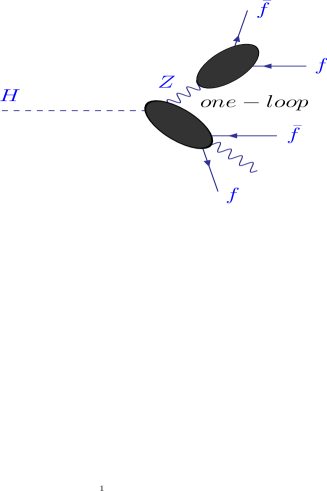
Figure 14: $H\to 4\mu$ in the single resonance
approximation.

In our generator we implement two building blocks at the one-loop level: $H\to ffZ(\gamma)$ and $Z\to ff(\gamma)$. We merge these two blocks and create a link between them by means of the $Z^{*}$ (resonating boson) line with Breit-Wigner mass distribution. In this spirit we create the generator in the single resonance approximation. We also built a double resonance generator, where we incorporated resonance approximation in two $Z^{*}$ lines.

The range for application of the single resonance approximation was found to be $120$ GeV$\leq M_{\scriptscriptstyle{H}}\leq 160$ GeV and for the double resonance approximation $M_{\scriptscriptstyle{H}}\geq$ 180 GeV.

These conclusions are illustrated by Fig. 15 where we present the results of calculations of the tree level width of the decay $H\to 4\mu$ for the three cases:
1) solid line: results of complete tree level calculations neglecting effects of identical final state muons;
2) dash dotted line: single resonance approximation,

$$\Gamma^{\rm{1-res}}_{H\to 4\mu}=\frac{\Gamma_{H\to 2\mu Z}\Gamma_{Z\to 2\mu}}{\Gamma_{Z}}\;;$$ (43)

3) dashed line: double resonance approximation,

$$\Gamma^{\rm{2-res}}_{H\to 4\mu}=\frac{\Gamma_{H\to 2Z}\Gamma^{2}_{Z\to 2\mu}}{\Gamma^{2}_{Z}}\;.$$ (44)

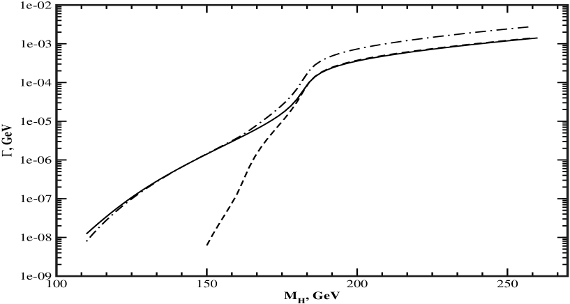
Figure 15: Born width of the decay $H\to 4\mu$ in three approximations.

The loop-corrected result is the linear combination of three types of events: Born with Identity events minus Resonanse Born events plus One-loop Resonance events. We feel that this is the main shortcoming of the generator.

Let us consider each type of events:

• ‘‘Born with Identity’’ events means a branch which computes the distributions without radiative corrections but with effects of identical muons;

• ‘‘Resonance Born’’ events means resonance approximation for one of the $Z$ bosons, i.e. $H\to ZZ^{*}\to\mu^{+}\mu^{-}\mu^{+}\mu^{-}$, where $Z^{*}$ is the resonating $Z$. Here, the two building blocks in Fig. 14 are calculated at the Born level;

• ‘‘Resonance One-loop’’ events is implemented in the same spirit as ‘‘Resonance Born’’, but building blocks $H\to ffZ(\gamma)$ and $Z\to ff(\gamma)$ are calculated at the one-loop level.

The codes of both MC generators can be obtained from the authors by request.

Recently appeared a new MC code Prophecy4f, see Refs.[11]--[12], realizing calculation of the complete one-loop corrected partial widths of the $H\to 4l$ channels. We present a preliminary comparison between MC Prophecy4f and SANC in Table 6.

$\sqrt{s}$, GeV	$120$	$130$	$140$	$150$	$160$
Prophecy4f	$7.053(3)\cdot 10^{-8}$	$2.3769(9)\cdot 10^{-7}$	$6.692(2)\cdot 10^{-7}$	$1.6807(6)\cdot 10^{-6}$	$4.006(1)\cdot 10^{-6}$
SANC ($G_{\mu}$)	$7.197(3)\cdot 10^{-8}$	$2.4079(8)\cdot 10^{-7}$	$6.743(2)\cdot 10^{-7}$	$1.6842(5)\cdot 10^{-6}$	$3.962(2)\cdot 10^{-6}$
$\delta,\%$	2.04	1.01	0.76	0.21	-1.10
SANC ($\alpha$)	$6.938(2)\cdot 10^{-8}$	$2.343(1)\cdot 10^{-7}$	$6.594(2)\cdot 10^{-7}$	$1.6534(5)\cdot 10^{-6}$	$3.915(1)\cdot 10^{-6}$

Table 6: Comparison for partial width for decay $H\to 4\mu$ in $G_{\mu}$ scheme for $M_{\scriptscriptstyle{H}}=140$ GeV between Prophecy4f and SANC.

As seen from the Table, there is $\pm$1% agreement in the mass range 130--140 GeV, degrading at the edges of the interval [120--160], that finds its natural explanation in Fig.15. Moreover, Prophecy4f uses the complex-mass scheme and takes into account several higher order corrections. One has to emphasize, however, that SANC calculations in $\alpha$ and $G_{\mu}$ schemes differ by about 2%. This can be considered as a rough estimate of the theoretical error. Prophecy4f numbers lie basically inside the range of SANC predictions.

The generator in the single resonance approximation described in this section was used for a MC simulation of $H\to 4\mu$ decay in the ATLAS detector and the results were compared with simulation by PYTHIA, showing notable deviations, see [22]. This fact demonstrates the importance of higher order corrections and the necessity to reduce the theoretical error.

8 User Guide

8.1 Benchmark case 3: the process $H\to f_{1}\bar{f_{1}}Z$

Here we consider the $2f2b$ NC process $H\to f_{1}\bar{f}_{1}Z$.

One can open the relevant branch of the SANC tree as follows:

EW $\to$ Processes $\to$ 4 legs $\to$ 2f2b $\to$ Neutral Current $\to$ H$\to$f1f1Z

For this process there are three FORM programs: (FF) Form Factors, (HA) Helicity Amplitudes, and (BR) Bremsstrahlung. Each of them in turn is opened, compiled and run as described in Section 6 of Ref.[1].

For the process $H\to e^{+}e^{-}Z$ we have in the Console window the particle indices shown in Table 7.

Table 7: Assignment of particle indices for the process $H\to e^{+}e^{-}Z$

typeIU = 44	initial partile (H-boson)
typeID = 12	final particle (electron)
typeFU = 12	final antiparticle (positron)
typeFD = 22	final particle (Z-boson)

These can be changed to typeID (typeFU) = 13,14 for up- and down-quarks in the final state of the processes $H\to(u{\bar{u}},d{\bar{d}})Z$ by editing the particle numbers as explained in Section 6 of Ref.[1]. .

Next bring the Fortran Editor sheet of the Editors List and the Numeric Form panel to the foreground. Shown in the Numeric Parameter sheet are the particle masses in GeV and the invariant mass of $f{\bar{f}}Z$ compaund in GeV, also the cosine of the angle $\vartheta_{l}$ defined in Fig.4.

Click on the Rehash button at the bottom of the Numeric Form panel: the main module of FORTRAN code appears in the Fortran Editor sheet of the Editors List. Then click on Compile. The final answer appears in the Output field. It consists of the parameters used ($\alpha$, $G_{F}$, particle masses, the ’t Hooft scale $\mu$ and the invariant mass of compaund), and the resulting differential width $d^{2}\Gamma/ds\,d\cos\vartheta_{l}$ in the Born approximation and Born+one-loop. The results for the default parameters and for several scattering angles are summarised in Table 8.

Table 8: The double differential widths for $H\to e^{+}e^{-}Z$ channel in $\alpha$-scheme: first row: the double differential decay width $d^{2}\Gamma/ds\,d\cos{\vartheta_{l}}\cdot 10^{8}$GeV^-1 at the Born level; second row: the double differential decay width at the 1-loop level; third row: relative correction $\delta=d^{2}\Gamma^{\rm{1-loop}}/d^{2}\Gamma^{\rm{Born}}$. Numerical values are truncated to 6 figures.

$H\to e^{+}e^{-}Z$
phantomphantom       Part 1, $d^{2}\Gamma/ds\,d\cos{\vartheta_{l}}\cdot 10^{8}$, GeV-1
	$\sqrt{s}$, GeV	$1$	$3$	$10$	$28$
Born		$0.02019$	$0.02144$	$0.03505$	$0.04261$
1-loop	$\cos{\vartheta_{l}}=\pm 0.9$	$0.21060$	$0.04321$	$0.03874$	$0.04602$
$\delta$		$9.43022$	$1.01508$	$0.10537$	$0.07984$
Born		$0.07914$	$0.07964$	$0.08478$	$0.04353$
1-loop	$\cos{\vartheta_{l}}=\pm 0.5$	$0.21495$	$0.09898$	$0.09150$	$0.04701$
$\delta$		$1.71589$	$0.24281$	$0.07922$	$0.07976$
Born		$0.10546$	$0.10562$	$0.10698$	$0.04394$
1-loop	$\cos{\vartheta_{l}}=\phantom{-}0.0$	$0.21695$	$0.12394$	$0.11510$	$0.04745$
$\delta$		$1.05716$	$0.17343$	$0.07586$	$0.07972$

Input parameters can be changed by editing the appropriate field of the Numeric Form panel and pressing the Rehash button. Again the Rehash button must be pressed before pressing Compile.

To produce whole Table 8 one can set flag tbprint = 1 in the Fortran Editors sheet. After editing the code just press Compile; there is no need to press the Rehash button.

One can also produce the differential width $d\Gamma/ds$ and total width $\Gamma$ in GeV by integrating the above differential width. To produce these numbers one can set flag inflag = 1,2, respectevely, in the Fortran Editors sheet. After editing the code just press Compile; again, there is no need to press the Rehash button.

Acknowledgments

The authors are grateful to P. Christova for a valuable discussion of bremsstrahlung issues, to A. Arbuzov for discussion of the stability of numerical calculations and physical results and also to W. Hollik for providing us with useful references. Three of us (D.B., L.K. and G.N.) are cordially indebted to S. Jadach and Z. Was for offering us an opportunity of encouraging common work at IFJ Krakow in April--May 2005 and to the IFJ directorate for hospitality which was extended to us in this period, when the major part of this study was done. We are thankful to the authors of the Prophecy4f generator for providing us with their numbers for Table 6.

References

- [1] A. Andonov et al., Comput. Phys. Commun. 174 (2006) 481--517.
- [2] A. Arbuzov et al., Eur. Phys. J. C 46 (2006) 407.
- [3] R. Sadykov, et al., in proceedings of "International Workshop of Top Quark Physics", PoS (TOP2006) 036.
- [4] A. Arbuzov, D. Bardin, S. Bondarenko, P. Christova, L. Kalinovskaya, G. Nanava, R. Sadykov, and W. von Schlippe, SANCnews: Sector 4f, Charged Current, to appear in EPJC, ‘‘DOI 10.1140/epjc’’, hep-ph/0703043.
- [5] D. Bardin, S. Bondarenko, L. Kalinovskaya, G. Nanava and L. Rumyantsev, The three channels of the process in the SANC framework, to be published in EPJC, hep-ph/0702115.
- [6] D. Bardin, L. Kalinovskaya, V. Kolesnikov and E. Uglov, Light-by-light scattering in SANC, Talk presented at the International School-Seminar CALC2006, Dubna, 15-25 July 2006, hep-ph/0611188.
- [7] A. Andonov, A. Arbuzov, S. Bondarenko, P. Christova, V. Kolesnikov and R. Sadykov, QCD branch in SANC, to appear in ‘‘Particles and Nuclei Letters’’ N5, 2007. hep-ph/0610268.
- [8] A. Denner and T. Sack, Nucl. Phys. B 306 (1988) 221,
- [9] M. L. Ciccolini, S. Dittmaier and M. Kramer, Phys. Rev. D 68 (2003) 073003.
- [10] O. Brein et al., Precision Calculations for Associated WH and ZH Production at Hadron Colliders, Contributed to 3rd Les Houches Workshop: Physics at TeV Colliders, hep-ph/0402003.
- [11] A. Bredenstein, A. Denner, S. Dittmaier and M. M. Weber, Precise predictions for the Higgs-boson decay H WW/ZZ 4 leptons, hep-ph/0604011.
- [12] C. Buttar et al., Les Houches physics at TeV colliders 2005, standard model, QCD, EW, and Higgs working group: Summary report, hep-ph/0604120.
- [13] J. A. M. Vermaseren, New features of FORM, math-ph/0010025.
- [14] D. Bardin and G. Passarino, The standard model in the making: Precision study of the electroweak interactions. Clarendon, 1999. Oxford, UK.
- [15] T. Kinoshita, J. Math. Phys. 3 (1962) 650.
- [16] T. D. Lee and M. Nauenberg, Phys. Rev. B 133 (1964) 1549.
- [17] T. Hahn and M. Perez-Victoria, Comput. Phys. Commun. 118 (1999) 153.
- [18] A. Denner, J. Kublbeck, R. Mertig and M. Bohm, Z. Phys. C 56 (1992) 261.
- [19] G. Belanger et al., Phys. Rept. 430 (2006) 117.
- [20] M. Bohm and T. Sack, Z. Phys. C 35 (1987) 119.
- [21] URL: http://pdg.lbl.gov/2006/tables/contents_tables.html.
-
[22]
I. Boyko, Full simulation study of Higgs bosons produced with SANC generator,
the talk at ATLAS Higgs Working Group meeting, 19 April 2006.
URL: http://indico.cern.ch/conferenceDisplay.py?confId=a058301.