Large Non-perturbative Effects of Small $\Delta m^{2}_{21}/\Delta m^{2}_{31}$ and $\sin\theta_{13}$
on Neutrino Oscillation and CP Violation in Matter

Abstract

In the framework of three generations, we consider the CP violation in neutrino oscillation with matter effects. At first, we show that the non-perturbative effects of two small parameters, $\Delta m_{21}^{2}/\Delta m_{31}^{2}$ and $\sin\theta_{13}$, become more than $50\%$ in certain ranges of energy and baseline length. This means that the non-perturbative effects should be considered in detailed analysis in the long baseline experiments. Next, we propose a method to include these effects in approximate formulas for oscillation probabilities. Assuming the two natural conditions, $\theta_{23}=45^{\circ}$ and the fact that the matter density is symmetric, a set of approximate formulas, which involve the non-perturbative effects, has been derived in all channels.

1 Introduction

Last year, the direct evidence for neutrino oscillation [1] was found in three kinds of experiments, namely atmospheric neutrino experiment [2], reactor neutrino experiment [3] and K2K experiment [4]. In these experiments, the dip of neutrino oscillation and the energy dependence of the probability, were observed. The possibilities of neutrino decay [5] and neutrino decoherence [6] are excluded by these results and it is found that the only solution for the solar and the atmospheric neutrino problem is neutrino oscillation. The observation of the dip also means that the neutrino experiments herald in a new era of precise measurements, because the effect, which disappears by averaging out the time-varying part on the neutrino energy, has been observed in these experiments for the first time [2, 3, 4]. Solar neutrino parameters have been also accurately determined by recent neutrino experiments such as SNO and KamLAND [7, 8].

From the results of the past experiments, it was found that the solar neutrino deficit is explained by the Large Mixing Angle (LMA) MSW [9] solution [7, 8, 10, 11],

$$\Delta m_{21}^{2}\sim 8.0\times 10^{-5}{\rm eV^{2}},\qquad\sin^{2}2\theta_{12}\simeq 0.8,$$ (1.1)

where the mass squared difference is defined by $\Delta m_{ij}^{2}=m_{i}^{2}-m_{j}^{2}$. It was obtained that

$$|\Delta m_{31}^{2}|\sim 2.0\times 10^{-3}{\rm eV^{2}},\qquad\sin^{2}2\theta_{23}\simeq 1.0$$ (1.2)

from the atmospheric neutrino experiment [12]. Furthermore, the upper bound of the 1-3 mixing angle, $\sin\theta_{13}$ is given by

$$\sin^{2}2\theta_{13}\leq 0.2$$ (1.3)

from the reactor experiment [13]. The next step for neutrino physics is the determination of $\sin\theta_{13}$, the sign of $\Delta m_{31}^{2}$ and CP phase $\delta$. In particular, the measurement of the leptonic CP phase is one of the most important themes from the viewpoint of the origin of the universe. CP violation has been investigated also in quark sector for the first time and the Kobayashi-Maskawa theory has been established [14]. However, it has been found that the CP violation in quark sector is too small to generate the sufficient baryon number in the universe [15], because the electroweak symmetry breaking is not the first phase transition as the Higgs particle is too heavy. This means that the origin of baryon asymmetry of the universe is not a CP violation from the KM phase and an extra source of CP violation is needed. One of the alternatives is the generation of a baryon number due to the leptonic CP violation [16]. The possibility of this scenario has been investigated by many researchers [17].

In order to attain the next step, the long baseline experiments like superbeam experiments [18] and neutrino factory experiments [19] are planned. In these experiments, the earth matter effects disturb the observation of the CP violation because the matter in the earth is not CP invariant and generate the effects of fake CP violation. Therefore, it is very important to understand the earth matter effects in neutrino oscillation experiments.

Here, summarizing the results of the atmospheric, solar and reactor neutrino experiments, there are two small parameters

$$\alpha=\frac{\Delta m_{21}^{2}}{\Delta m_{31}^{2}} \sim 0.04,$$ (1.4)

$$s_{13}=\sin\theta_{13} \leq 0.23.$$ (1.5)

The magnitude of these small parameters is most important for measuring the CP violation, because it cannot be observed, if one of these parameters vanishes. As the LMA MSW solution was chosen to explain the results of the solar neutrino experiments, $\alpha$ reduced to the largest value compared to other solutions. This means that the LMA MSW solution opens the door for measuring the leptonic CP violation. If $s_{13}$ is too small, it will be impossible to observe the CP violation. Therefore the magnitude of $s_{13}$ controls whether the leptonic CP violation can be observed or not.

Let us briefly review the approximate formulas using the small parameter $\alpha$ or $s_{13}$ and the related papers. At first using the perturbation of oscillation probability in $\alpha$, the magnitude of the fake CP violation by the matter effects has been investigated in [20, 21, 22, 23, 24]. Furthermore, by expanding the matter potential to the Fourier mode, it has been shown in [25, 26] that the mode with large wavelength mainly contributes to the oscillation probability. Higher order perturbative calculations have been performed by [27, 28]. The perturbation in $s_{13}$ has been investigated in [29]. The perturbation in both $\alpha$ and $s_{13}$ has also been studied in [30, 31] and this method has been extended to all channels in [32].

Next let us review the remarkable features related to the leptonic CP violation. In the case of constant matter density, the notable identity $\tilde{J}\tilde{\Delta}_{12}\tilde{\Delta}_{23}\tilde{\Delta}_{31}=J\Delta_{12}\Delta_{23}\Delta_{31}$ has been found in [33, 34, 35], where $J$ is the Jarlskog factor related to the leptonic CP violation, $\Delta_{ij}$ means $\Delta m^{2}_{ij}/(2E)$ and tilde stands for the quantities in matter. In addition, it has been pointed out that the oscillation probability in matter almost coincide with that in vacuum under the certain condition, which is called vacuum mimicking phenomena, and the method to solve the problem on the fake CP violation by using the phenomena is discussed in detail [36, 37, 38]. Furthermore, it can be applied to the future long baseline experiments by using the statistical method explained by [39, 40].

In a previous series of papers [41, 42, 43, 44, 45] we have considered the three generation neutrino oscillation in matter and have shown that the CP dependence of the oscillation probabilities are derived exactly [41]. In the case that $\nu_{e}$ is included in the initial or final state, the CP dependence is given by

$$P(\nu_{e}\to\nu_{e}) = C_{ee},$$ (1.6)

$$P(\nu_{\alpha}\to\nu_{\beta}) = A_{\alpha\beta}\cos\delta+B_{\alpha\beta}\sin\delta+C_{\alpha\beta},$$ (1.7)

and in the case that both the initial and final state are $\nu_{\alpha},\nu_{\beta}=\nu_{\mu},\nu_{\tau}$, the CP dependence is given by

$$P(\nu_{\alpha}\to\nu_{\beta}) = A_{\alpha\beta}\cos\delta+B_{\alpha\beta}\sin\delta+C_{\alpha\beta}+D_{\alpha\beta}\cos 2\delta+E_{\alpha\beta}\sin 2\delta,$$ (1.8)

where the coefficients $A_{\alpha\beta}\sim E_{\alpha\beta}$ are independent of the CP phase. We have also shown that these coefficients can be calculated exactly in constant matter and then the approximate formulas are derived in a simple way [42, 43]. Furthermore, we proposed a new method for approximating these coefficients in the case of non-constant matter density [44], and then applied it to the earth matter [45].

In this paper, at first within the framework of two generations, it has been shown that perturbation of the small mixing angle is not effective near the MSW resonance point. This means that the non-perturbative effects by the small mixing angle is important in the MSW resonance region. Next, we consider non-perturbative effects of $\Delta m_{21}^{2}/\Delta m_{31}^{2}$ and $\sin\theta_{13}$ in the three generation neutrino oscillation. The importance of the non-perturbative effects is shown by comparing the exact numerical calculation with the perturbative expansion of the small parameters. Furthermore, we consider the method for deriving the approximate formulas in which the non-perturbative effects are taken into account. In our previous paper [44], the approximate formulas for $P(\nu_{e}\to\nu_{\mu})$ have been derived. These formulas are effective for both MSW resonance regions. However, there is a problem because this method cannot be extended to other channels $P(\nu_{\mu}\to\nu_{\tau})$ and so on. In order to solve this problem, we assume the two natural conditions, $\theta_{23}=45^{\circ}$ and the symmetric matter potential. Under these conditions, we derive the approximate formulas for all channels, including non-perturbative effects of the two small parameters. These formulas are useful to solve the problem of parameter degeneracy.-

2 Non-perturbative Effect by Small Mixing Angle

In this section, we discuss the perturbative expansion of a small mixing angle in two generation neutrino oscillation. Although we discussed the perturbation of small parameters in our previous papers [44, 45], in order to clarify the physical meaning, we consider the perturbation due to a small mixing angle within the framework of two generations. Then, we show that the perturbation breaks down in the MSW resonance region even if the mixing angle is small.

2.1 MSW Resonance of Probability in Two Generations

In this subsection, we consider the two generation neutrino oscillation and we choose the energy region and the baseline length in which the MSW resonance occurs. Let us start from the Hamiltonian in constant matter

$$H = O{\rm diag}(0,\Delta)O^{T}+{\rm diag}(a,0)$$ (2.1)

$$= \tilde{O}{\rm diag}(\lambda_{1},\lambda_{2})\tilde{O}^{T},$$ (2.2)

where the matter potential is defined by $a=\sqrt{2}G_{F}N_{e}$. $G_{F}$ is the Fermi constant and $N_{e}$ is the electron density in matter. The matrix $O$ is mixing matrix as

$$O=\left(\begin{array}[]{cc}\cos\theta&\sin\theta\\ -\sin\theta&\cos\theta\end{array}\right),$$ (2.5)

where $\Delta=\Delta m^{2}/2E$ and the quantities with tilde stand for the quantities in matter. Diagonalizing (2.1) to (2.2), the effective masses $\lambda_{i}(i=1,2)$ and effective mixing angle $\tilde{\theta}$ are determined. If we use the notation $\tilde{\Delta}=\lambda_{2}-\lambda_{1}$ as the mass squared difference, there is a relation between the mass squared difference and the mixing angles as

$$\frac{\tilde{\Delta}}{\Delta}=\frac{\sin 2\theta}{\sin 2\tilde{\theta}}=\sqrt{\left(\cos 2\theta-\frac{a}{\Delta}\right)^{2}+\sin^{2}2\theta}.$$ (2.6)

Using these quantities in matter, the oscillation probability is given by

$$P=\sin^{2}2\tilde{\theta}\sin^{2}\frac{\tilde{\Delta}L}{2}.$$ (2.7)

The oscillating part with $L/E$ of this probability becomes large if the condition

$$\sin\frac{\tilde{\Delta}L}{2}\sim 1$$ (2.8)

is satisfied. On the other hand, the condition for the maximal effective mixing angle is given by

$$\sin 2\tilde{\theta}\sim 1.$$ (2.9)

In the case of small mixing angle, this condition is rewritten as $a=\Delta\cos 2\theta\sim\Delta$, and furthermore we define the resonance energy by

$$E\sim\frac{\Delta m^{2}}{2a}.$$ (2.10)

We also define the resonance length by

$$L\sim\frac{1}{a\sin\theta}.$$ (2.11)

For the case of $\sin\theta=0.16$, which is the upper bound in the CHOOZ experiment, the resonance length is roughly estimated as 10000 km. This means that in near future it is impossible to realize the long baseline experiments such that the baseline length from beam source to the detector is nearly equal to the resonance length. However, it has been shown [38] that matter effects exist even if the baseline length is shorter than the resonance length. Therefore, we use $L=6000$ km as the baseline length in the later sections.

2.2 Perturbation due to Small Mixing Angle

Next, let us consider the expansion of the effective mass $\tilde{\Delta}$ and the effective mixing angle $\sin 2\tilde{\theta}$ by a small mixing angle $\sin\theta$. We show that although the effective mass and the effective mixing angle diverge in the MSW resonance energy region, the oscillation probability, which is a function of these two quantities, converges.

At first, the effective mass is expanded as

$$\tilde{\Delta}=|\Delta-a|+\frac{2a\Delta}{|\Delta-a|}\sin^{2}\theta+\frac{a^{2}\Delta^{2}}{2|\Delta-a|^{3}}\sin^{4}\theta+\cdots.$$ (2.12)

One can see from this result that other terms than the first term diverge. The higher order term have larger divergence near the MSW resonance. The effective mixing angle is expanded as

$$\sin 2\tilde{\theta}=\frac{\Delta\sin 2\theta}{|\Delta-a|}\left(1-\frac{2a\Delta}{(\Delta-a)^{2}}\sin^{2}\theta+\frac{3a^{2}\Delta^{2}}{2(\Delta-a)^{4}}\sin^{4}\theta+\cdots\right).$$ (2.13)

The condition

$$\sin\theta<\frac{|\Delta-a|}{2\sqrt{a\Delta}}$$ (2.14)

is needed for $\sin 2\tilde{\theta}$ to converge the finite value. However, this condition cannot be satisfied in the MSW resonance region defined by $\Delta\sim a$, even if $\sin\theta$ is small. This means that the above perturbation series diverges. In the expansion for the effective mass and the effective mixing angle, the coefficients become large, even if these quantities are expanded by the small mixing angle.

Next, let us consider the oscillation probability and let us demonstrate that the oscillation probability reaches a finite value, where the divergences due to the effective mass and the effective mixing angle are canceled out by each other. Substituting (2.12) and (2.13) into (2.7), we obtain

$$P \sim \frac{\Delta^{2}\sin^{2}2\theta}{(\Delta-a)^{2}}\sin^{2}\frac{(\Delta-a)L}{2}$$ (2.15)

$$+ \frac{\Delta^{2}\sin^{2}2\theta}{(\Delta-a)^{2}}\left[-\frac{4a\Delta\sin^{2}\theta}{(\Delta-a)^{2}}\sin^{2}\frac{(\Delta-a)L}{2}+\frac{a\Delta L\sin^{2}\theta}{\Delta-a}\sin(\Delta-a)L\right]+\cdots.$$

In the limit, $\Delta\sim a$, it is found that the oscillation probability becomes finite as

$$P \sim \cos^{2}\theta\left(\sin^{2}\theta a^{2}L^{2}-\frac{1}{3}\sin^{4}\theta a^{4}L^{4}+\cdots\right).$$ (2.16)

From this equation, the oscillation probability becomes finite and the perturbation is a good approximation if

$$L<\frac{1}{a\sin\theta}.$$ (2.17)

As you see from (2.11), this is the condition that the baseline length is shorter than the resonance length.

Next, let us investigate the magnitude of non-perturbative effects numerically. We use the following parameters, $\Delta m^{2}=2.0\times 10^{-3}~{}{\rm eV^{2}}$ and $\sin\theta=0.16$. We set the baseline length, $L=6000~{}{\rm km}$ and the energy region, $1~{}{\rm GeV}\leq E\leq 50~{}{\rm GeV}$, to include the MSW resonance energy. Furthermore we choose a density of $\rho=4~{}{\rm g/cm^{3}}$.

(a) Level crossing	(b) Probability

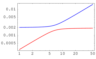
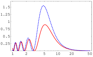
Figure 1: Comparison of the perturbative value with the exact one in the two generation neutrino oscillation probability. In (a), the energy dependence of two eigenvalues is plotted. In (b), the dotted and solid line show the values by the perturbative and numerical calculations, respectively.

At first, in figure 1(a) the level crossing of two eigenvalues is plotted. It is shown that the crossing energy is about 6-7 GeV, which corresponds to the MSW resonance energy. Next, in figure 1(b) we compare the oscillation probability calculated by perturbation with the one by numerical calculation. These figures show that the perturbation breaks down around the MSW resonance energy. The results of this subsection are summarized as

1. The perturbative expansion in the small mixing angle breaks down around the MSW resonance because the perturbation because the perturbation series diverges. The coefficients of this expansion become larger around the MSW resonance. The divergence included in the effective mass cancels with that in the effective mixing angle, and as a result, the value of the oscillation probability reaches a finite value. Term of eq. (2.12) and (2.13) cancel with each other.

2. Although the divergences of the effective mass and the effective mixing angle in the perturbative expansion cancel in the oscillation probability, the finite value of the probability differs from that by numerical calculation. The perturbation around the MSW resonance energy becomes a good approximation, if the baseline length is shorter than the resonance length as seen from (2.17). However, we need to take higher order terms of the perturbation into account, when the baseline length is longer, namely when non-perturbative effects become important.

3 Extension of method to Approximate Oscillation Probabilities

In this section, we consider the matter effects in three generation neutrino oscillation. At first, we review that the 2-3 mixing angle $\theta_{23}$ and the CP phase $\delta$ can be separated from matter effects in the oscillation probability [41]. This means that the matter effects appear through the remained four parameters. Furthermore, these four parameters can be separated to two set of parameters and each set is related to the phenomena in low and high energy as

$$(\theta_{12},\Delta m^{2}_{21}):{\rm Low~{}Energy~{}Phenomenon}$$ (3.1)

$$(\theta_{13},\Delta m^{2}_{31}):{\rm High~{}Energy~{}Phenomenon}.$$ (3.2)

This separation means that the parameters for the solar neutrino and those for the atmospheric neutrino are almost independent to each other. We propose the method deriving the approximate formulas simply by using this feature.

3.1 Definition of Low and High Energy Regions

In this subsection, we define the low energy and the high energy Hamiltonians in the small quantity limit when $s_{13}$ or $\alpha$ approximate zero. Although these Hamiltonian have been already introduced in our earlier papers [44, 45], we review them here, as they are used in later section.

It is noted that $H(t)$ satisfies the relation

$$H(t)=O_{23}\Gamma H^{\prime}(t)\Gamma^{\dagger}O_{23}^{T}$$ (3.3)

where $H^{\prime}$ is given by

$$H^{\prime}=O_{13}O_{12}{\rm diag}(0,\Delta_{21},\Delta_{31})O_{12}^{T}O_{13}^{T}+{\rm diag}(a(t),0,0).$$ (3.4)

This means that the 1-2 and 1-3 mixing angles are separated from the 2-3 mixing and the CP phase, as explained in detail in Appendix A. In this Appendix A, we derive the same result as that derived from this section from another point of view. Taking the limit $s_{13}\to 0$, the Hamiltonian reduces to the two generation Hamiltonian as

$$H^{\ell} = \lim_{s_{13}\to 0}H^{\prime}$$ (3.5)

$$= O_{12}{\rm diag}(0,\Delta_{21},\Delta_{31})O_{12}^{T}+{\rm diag}(a(t),0,0)$$ (3.6)

$$= \left(\begin{array}[]{ccc}\Delta_{21}s_{12}^{2}+a(t)&\Delta_{21}s_{12}c_{12}&0\\ \Delta_{21}s_{12}c_{12}&\Delta_{21}c_{12}^{2}&0\\ 0&0&\Delta_{31}\end{array}\right)$$ (3.10)

This means that the third generation is now separated from the first and the second generation. As seen from this Hamiltonian (3.10), the components except for $H_{\tau\tau}^{\ell}$, depend only on $(\theta_{12},\Delta_{21})$. We call $H^{\ell}$ the low energy Hamiltonian. On the other hand, taking the limit $\alpha\to 0$, the Hamiltonian reduces to the two generation Hamiltonian as

$$H^{h} = \lim_{\alpha\to 0}H^{\prime}$$ (3.11)

$$= O_{13}{\rm diag}(0,0,\Delta_{31})O_{13}^{T}+{\rm diag}(a(t),0,0)$$ (3.12)

$$= \left(\begin{array}[]{ccc}\Delta_{31}s_{13}^{2}+a(t)&0&\Delta_{31}s_{13}c_{13}\\ 0&0&0\\ \Delta_{31}s_{13}c_{13}&0&\Delta_{31}c_{13}^{2}\end{array}\right).$$ (3.16)

This means that the second generation is also separated from the two others. This Hamiltonian (3.16) is expressed by only the parameters $(\theta_{13},\Delta_{31})$. We call $H^{h}$ high energy Hamiltonian. Next, let us define the high and low energy regions described by $H^{h}$ and $H^{\ell}$. We first calculate the MSW resonance energy because the MSW effect is the most important in matter effects. In the case of $L=6000~{}{\rm km}$, which we use later, the average matter potential is calculated as $\rho=3.91~{}{\rm g/cm^{3}}$. By using this value, we obtain the high energy MSW resonance as $E^{h}=\Delta m_{31}^{2}/a\simeq 5~{}{\rm GeV}$ and the low energy MSW resonance as $E^{\ell}=\Delta m_{21}^{2}/a\simeq 0.2~{}{\rm GeV}$. From these results, we regard $E\sim 1{\rm GeV}$ as the boundary energy of low and high energy regions. Therefore, we define the high as $E\geq 1~{}{\rm GeV}$ and the low energy regions as $E\leq 1~{}{\rm GeV}$.

3.2 Order Counting of Amplitude on $\alpha$ and $s_{13}$

In this subsection, we investigate how the amplitude $S^{\prime}$, which is defined by the primed Hamiltonian (3.4), depends on the two small parameters $\alpha$ and $s_{13}$. Before, we have already clarified some general features of $S^{\prime}$ related to the order of $\alpha$ and $s_{13}$, and the dependences on $s_{13}$ and $\alpha$ for particular amplitudes $S^{\prime}_{\mu e}$ and $S^{\prime}_{\tau e}$ have been given in our previous papers [44, 45]. We investigate now the dependences on $s_{13}$ and $\alpha$ for all amplitudes.

At first, we represent the explicit form of the Hamiltonian, when the 2-3 mixing angle and the CP phase are factored out as

$$H^{\prime}(t) = O_{13}O_{12}{\rm diag}(0,\Delta_{21},\Delta_{31})O_{12}^{T}O_{13}^{T}+{\rm diag}(a(t),0,0)$$ (3.17)

$$= \left(\begin{array}[]{ccc}\Delta_{21}c_{13}^{2}s_{12}^{2}+\Delta_{31}s_{13}^{2}+a(t)&\Delta_{21}c_{13}s_{12}c_{12}&-\Delta_{21}c_{13}s_{13}s_{12}^{2}+\Delta_{31}s_{13}c_{13}\\ \Delta_{21}c_{13}s_{12}c_{12}&\Delta_{21}c_{12}^{2}&-\Delta_{21}s_{13}s_{12}c_{12}\\ -\Delta_{21}c_{13}s_{13}s_{12}^{2}+\Delta_{31}s_{13}c_{13}&-\Delta_{21}s_{13}s_{12}c_{12}&\Delta_{21}s_{13}^{2}s_{12}^{2}+\Delta_{31}c_{13}^{2}\end{array}\right).$$ (3.21)

The components of this Hamiltonian depend on $\alpha$ and $s_{13}$ as

$$H^{\prime}(t) = \left(\begin{array}[]{ccc}O(1)&O(\alpha)&O(s_{13})\\ O(\alpha)&O(\alpha)&O(\alpha s_{13})\\ O(s_{13})&O(\alpha s_{13})&O(1)\end{array}\right).$$ (3.25)

From this result, we can see that non-diagonal components are small compared to the diagonal components. We also understand that $H^{\prime}_{\mu\tau}$ is the smallest component and $H^{\prime}_{e\mu},H^{\prime}_{e\tau}$ are the next smaller components. We should note the salient feature that the result of this order counting holds in $H^{n}$ for arbitrary $n$. Namely, we obtain

$$(H^{\prime}(t))^{n} = \left(\begin{array}[]{ccc}O(1)&O(\alpha)&O(s_{13})\\ O(\alpha)&O(\alpha^{2})&O(\alpha s_{13})\\ O(s_{13})&O(\alpha s_{13})&O(1)\end{array}\right)\quad{\rm for}\quad n=1,2,\cdots.$$ (3.29)

According to this result, the order of the amplitude $S^{\prime}(t)$ for two small parameters $\alpha$ and $s_{13}$ is given by

$$S^{\prime}(t)={\rm T}\exp\left\{-i\int H^{\prime}(t)dt\right\}=\left(\begin{array}[]{ccc}O(1)&O(\alpha)&O(s_{13})\\ O(\alpha)&O(1)&O(\alpha s_{13})\\ O(s_{13})&O(\alpha s_{13})&O(1)\end{array}\right).$$ (3.33)

This result is almost the same as that of the original Hamiltonian. Furthermore, we consider the general features derived from the original Hamiltonian. The $\theta_{13}$ dependence of this Hamiltonian is described as

$$H^{\prime}=\left(\begin{array}[]{ccc}{\rm even}&{\rm even}&{\rm odd}\\ {\rm even}&{\rm even}&{\rm odd}\\ {\rm odd}&{\rm odd}&{\rm even}\end{array}\right)$$ (3.34)

and this dependence does not change for $(H^{\prime})^{n}$, because

$$(H^{\prime})^{n}=\left(\begin{array}[]{ccc}{\rm even}&{\rm even}&{\rm odd}\\ {\rm even}&{\rm even}&{\rm odd}\\ {\rm odd}&{\rm odd}&{\rm even}\end{array}\right)\quad{\rm for}\quad n=1,2,\cdots.$$ (3.35)

Due to this result, the amplitude $S^{\prime}(t)$ has the same structure,

$$S^{\prime}={\rm T}\exp\left\{-i\int H^{\prime}(t)dt\right\}=\left(\begin{array}[]{ccc}{\rm even}&{\rm even}&{\rm odd}\\ {\rm even}&{\rm even}&{\rm odd}\\ {\rm odd}&{\rm odd}&{\rm even}\end{array}\right).$$ (3.39)

This is a general feature, which holds in arbitrary matter profile.

3.3 Proposal of Simple Method

In the previous subsection, we have shown the general features (3.33) and (3.39) for the amplitude $S^{\prime}(t)$ related to the almost vanishing parameters $s_{13}$ and $\alpha$. However, we cannot calculate $S^{\prime}(t)$ by using only this features. In this subsection, we propose a generalized method for the calculation. Let us consider if there is an approximation available for both region, low and high energy. After expanding the amplitude $S^{\prime}$ on the two small parameters $\alpha$ and $s_{13}$, we can arrange this as

$$S^{\prime} = O(1)+O(\alpha)+O(s_{13})+O(\alpha^{2})+O(\alpha s_{13})+O(s_{13}^{2})+\cdots$$

$$= \Big{(}O(1)+O(\alpha)+O(\alpha^{2})+\cdots\Big{)}+\Big{(}O(1)+O(s_{13})+O(s_{13}^{2})+\cdots\Big{)}$$

$$- O(1)+O(\alpha s_{13})+O(\alpha^{2}s_{13})+O(\alpha s_{13}^{2})+\cdots$$ (3.41)

$$= \lim_{s_{13}\to 0}S^{\prime}+\lim_{\alpha\to 0}S^{\prime}-\lim_{\alpha,s_{13}\to 0}S^{\prime}+O(\alpha s_{13})+O(\alpha^{2}s_{13})+\cdots$$ (3.42)

$$= S^{\ell}+S^{h}-S^{d}+O(\alpha s_{13})+O(\alpha^{2}s_{13})+O(\alpha s_{13}^{2})+\cdots,$$ (3.43)

where $S^{\ell},S^{h}$ and $S^{d}$ are defined by

$$S^{\ell} = \lim_{s_{13}\to 0}S^{\prime}={\rm T}\exp\left\{-i\int H^{\ell}dt\right\}$$ (3.44)

$$S^{h} = \lim_{\alpha\to 0}S^{\prime}={\rm T}\exp\left\{-i\int H^{h}dt\right\}$$ (3.45)

$$S^{d} = \lim_{\alpha,s_{13}\to 0}S^{\prime}={\rm diag}\left(\exp\left\{-i\int a(t)dt\right\},1,e^{-i\Delta_{31}L}\right),$$ (3.46)

respectively. $S^{\ell}$ ($S^{h}$) corresponds to the amplitudes, which gives the main contribution in low (high) energy. The term $S^{d}$ counts twice, because contributions to this term comes from both, low energy and high energy terms. Therefore, we subtract this contribution and approximate the amplitude as

$$S^{\prime}\sim S^{\ell}+S^{h}-S^{d}$$ (3.47)

ignoring higher order terms. Let us discuss this approximation, which is used to derive our main result here.

In (3.3)-(3.43), the higher order terms in $\alpha$ and $s_{13}$ are included in $S^{\ell}$ and $S^{h}$. The reason for including the higher order terms is to take into account non-perturbative effects, which become important in the low and high energy MSW resonance region as discussed in section 2. On the other hand, we ignore those higher order terms, which are proportional to both $\alpha$ and $s_{13}$. For example, in the case of second order of the small parameters, $\alpha$ and $s_{13}$, we ignore only the mixed $O(\alpha s_{13})$ term among the three terms with second order $O(\alpha^{2}),O(s_{13}^{2})$ and $O(\alpha s_{13})$. This procedure is more appropriate than the usual perturbation, because both non-perturbative effects on a small $\alpha$ in the low energy region and on a small $s_{13}$ in the high energy region can be included in our approximation. However, as the derivation of the approximation (3.47) is not exact, we need to check this later numerically. In the previous subsection, the parity of the matrix elements related to $s_{13}$ has been derived. The equations (3.33), (3.39) and (3.47) lead to the magnitude of the correction for the amplitudes as

$$S^{\prime}_{\mu e} = S^{\ell}_{\mu e}+O(\alpha s_{13}^{2})$$ (3.48)

$$S^{\prime}_{\tau e} = S^{h}_{\tau e}+O(\alpha s_{13})$$ (3.49)

$$S^{\prime}_{\tau\mu} = O(\alpha s_{13})$$ (3.50)

$$S^{\prime}_{ee} = S^{\ell}_{ee}+S^{h}_{ee}-S^{d}_{ee}+O(\alpha s_{13}^{2})$$ (3.51)

$$S^{\prime}_{\mu\mu} = S^{\ell}_{\mu\mu}+O(\alpha s_{13}^{2})$$ (3.52)

$$S^{\prime}_{\tau\tau} = S^{h}_{\tau\tau}+O(\alpha s_{13}^{2}).$$ (3.53)

If we ignore the higher order terms which are proportional to both, $\alpha$ and $s_{13}$, in these equations, we obtain approximate formulas by using the two generation amplitudes. The main term for $S^{\prime}_{\mu e},S^{\prime}_{\mu\mu}$ is approximated by the low-energy amplitude as seen from (3.48) and (3.52). On the other hand, the main terms for $S^{\prime}_{\tau e}$ and $S^{\prime}_{\tau\tau}$ are approximated by the high-energy amplitude as derived from (3.49) and (3.53), and these features come from eq. (3.33). As seen from (3.48)-(3.53), these are expressed by only two generation amplitudes and have the advantage of simplicity. The precision of the approximation depends on the values of $s_{13}$ and $\alpha$. If the value of $s_{13}$ is smaller than the upper bound derived by the CHOOZ experiment, the precision of approximation becomes better. It should be mentioned that the method described in this subsection does not need the assumption of constant matter density.

Next, we show that the results using the approximate formulas (3.48)-(3.53) are in excellent agreement with the numerical calculations. We choose the Preliminary Reference Earth Model (PREM) as an earth matter density model and compare the amplitudes in all channels calculated from our approximate formulas with the numerical calculation. Here, $\Delta m_{21}^{2}=8.3\times 10^{-5}~{}{\rm eV^{2}},\Delta m_{31}^{2}=2.0\times 10^{-3}~{}{\rm eV^{2}},\sin^{2}2\theta_{12}=0.8$ and $\sin\theta_{13}=0.23$ are chosen. Furthermore, we set the baseline length as $L=6000~{}{\rm km}$, a length, for which the MSW effect becomes significant, and the energy region as $1~{}{\rm GeV}\leq E\leq 20~{}{\rm GeV}$, for which the MSW resonance energy appears.

$|S^{\prime}_{\mu e}|$	$|S^{\prime}_{\tau e}|$	$|S^{\prime}_{\tau\mu}|$
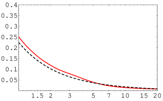
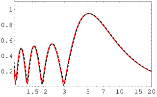
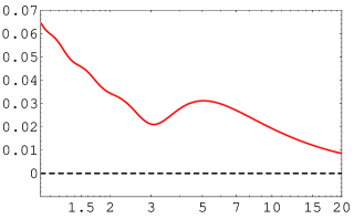
$|S^{\prime}_{ee}|$	$|S^{\prime}_{\mu\mu}|$	$|S^{\prime}_{\tau\tau}|$

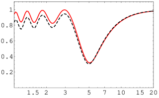
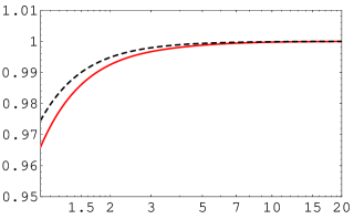
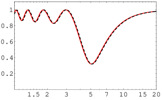
Figure 2: Comparison of our approximate formulas with the numerical calculation. In these figures the absolute value of the amplitudes in all channels is plotted in order to compare our formulas with numerical calculation. The solid lines show the approximate probabilities calculated from (3.48)-(3.53) and the dashed lines show the probabilities in the numerical calculation.

We compare our formulas with the numerical calculation in Figure 2. One can see in the following that some remarkable features occur. At first, the four amplitudes $|S^{\prime}_{\mu e}|,|S^{\prime}_{ee}|,|S^{\prime}_{\mu\mu}|$ and $|S^{\prime}_{\tau\tau}|$ coincide with the numerical calculation with a good precision. This happens, because there is no first order correction of $s_{13}$ from (3.48) and (3.51)-(3.53). Next, the low-energy part of $|S^{\prime}_{\tau e}|$ differs from the numerical calculation only a little, which can be understood from the eq. (3.49). Furthermore, our approximation for $|S^{\prime}_{\tau\mu}|$ is not at all in agreement with the numerical calculation. Although the value of this amplitude is exactly zero in our approximation as seen from (3.50), the actual magnitude of this amplitude attains $0.02$ in the low energy region from Figure 1. It is noted that this value is almost the same as the value expected from the order counting $O(\alpha s_{13})\sim 0.01$. Next, we would like to derive the approximate formulas of the oscillation probabilities from the amplitudes obtained here, however, there is a problem. As seen from eqs. (A.32)-(A.49) in Appendix A, we cannot obtain the approximate formulas for the CP dependence of the probabilities $P(\nu_{\mu}\to\nu_{\mu}),P(\nu_{\mu}\to\nu_{\tau})$ and $P(\nu_{\tau}\to\nu_{\tau})$. The reason is that the CP dependence in these channels is directly proportional to $S^{\prime}_{\mu\tau}$. However there is a method to calculate these indirectly by using the unitarity, even if we cannot directly obtain the amplitude $S^{\prime}_{\mu\tau}$, as we will show in section 4.

3.4 Discussion

In this subsection, let us reconsider the method proposed in the previous subsection in more detail. In (3.3)-(3.43), we ignored the terms of the order $O(\alpha s_{13})$ for the amplitude $S^{\prime}$. The reader probably wonder, why we ignore the terms of order $O(\alpha s_{13})$ for the amplitude $S^{\prime}$, but not for other quantities, like for example $H^{\prime}$ and $P$. Let us demonstrate the case of using the physical quantity $Q$. Expanding $Q$ on $\alpha$ and $s_{13}$, we obtain

$$Q=Q^{\ell}+Q^{h}-Q^{d}+O(\alpha s_{13})+O(\alpha^{2}s_{13})+\cdots$$ (3.54)

by the same procedure as (3.3)-(3.43). If we neglect the higher order terms like $O(\alpha s_{13})$, we can approximate $Q$ as

$$Q\sim Q^{\ell}+Q^{h}-Q^{d}.$$ (3.55)

As in the case of the approximated amplitude defined in the previous subsection, $Q^{\ell}=Q^{\ell}(\theta_{12},\Delta_{21})$ is the main term in low-energy and $Q^{h}=Q^{h}(\theta_{13},\Delta_{31})$ is the main term in high-energy. $Q^{d}$ is the double counting term. It is a method to be able to take into account non-perturbative effects in both of the two MSW resonance regions. In principle, this method is effective whatever we choose for the quantity $Q$, there is just a difference in simplicity and the magnitude of error, as discussed in the following.

We consider the Hamiltonian $H^{\prime}$ as $Q$. Namely, $H^{\prime}$ can be approximated as

$$H^{\prime}\sim H^{\ell}+H^{h}-H^{d},$$ (3.56)

where the double counting term is given by

$$H^{d}={\rm diag}\left(a(t),0,\Delta_{31}\right).$$ (3.57)

There is a problem, because approximation became too simple: The form of the solution for the amplitude is given by

$$S^{\prime}\sim{\rm T}\exp\left\{-i\int(H^{\ell}+H^{h}-H^{d})dt\right\},$$ (3.58)

and we cannot simplify this amplitude without calculation of the commutator of $H^{\ell}$ and $H^{h}$. Thus, the direct application of our method for the Hamiltonian needs other approximations to estimate the amplitude and this is not effective from the point of the simplicity. Especially, the amplitudes cannot be calculated within the framework of the two generation approximation although the precision of this approximation was good.

Next, let us consider the probability $P$ as the quantity $Q$. In this case, we can approximate as

$$P\sim P^{\ell}+P^{h}-P^{d},$$ (3.59)

where $P^{\ell}$ and $P^{h}$ are given by

$$P^{\ell(h)}=\left|{\rm T}\exp\left\{-i\int H^{\ell(h)}dt\right\}\right|^{2},$$ (3.60)

and $P^{d}$ is the identity matrix. As an example, we consider $P(\nu_{e}\to\nu_{\mu})$. The CP phase $\delta$ dependence is given by

$$P(\nu_{e}\to\nu_{\mu})=A_{e\mu}\cos\delta+B_{e\mu}\sin\delta+C_{e\mu},$$ (3.61)

where the coefficients $A_{e\mu}$ and $B_{e\mu}$ determine the magnitude of the CP violation. On the other hand, the CP violation becomes zero in the limit, $\alpha\to 0$ or $s_{13}\to 0$, as seen from

$$A_{e\mu}=O(\alpha s_{13}),\quad B_{e\mu}=O(\alpha s_{13}).$$ (3.62)

Namely, we obtain

$$A_{e\mu}^{\ell}=A_{e\mu}^{h}=A_{e\mu}^{d}=0,\quad B_{e\mu}^{\ell}=B_{e\mu}^{h}=B_{e\mu}^{d}=0$$ (3.63)

and therefore we cannot calculate quantities like the CP violation, because it is the effects of three generations in this approximation. This result holds for all channels.

To summarize this subsection, if we choose the Hamiltonian $H^{\prime}$ as $Q$, the precision of approximation is good, but the calculation is not so simple compared to the exact calculation. If we choose the probability $P$ as $Q$, we cannot calculate three generation effects like CP violation. On the other hand, if we choose the amplitude $S^{\prime}$ as $Q$, we can calculate the three generation effects like CP violation within the framework of two generation approximation.

4 Approximate Formulas for Oscillation Probabilities

In this section, we calculate the CP dependent terms from $\nu_{\mu}$ to $\nu_{\mu}$ and so on, not determined by the method in the previous section, by using the unitarity. After that, we derive the approximate formulas of the oscillation probabilities $P(\nu_{\alpha}\to\nu_{\beta})$ in arbitrary matter profile without using $S^{\prime}_{\mu\tau}$ directly. Namely, we derive the approximate formulas in all channels by our new method.

4.1 Unitarity Relation

We cannot calculate the amplitude $S^{\prime}_{\mu\tau}$ in the method introduced in the previous section. The reason is that the amplitude $S^{\prime}_{\mu\tau}$ is a very small quantity, which has an order of $O(\alpha s_{13})$. As seen from (A.32)-(A.49) in Appendix A, it seems that the approximate formulas, including CP violation, of three channels, $P(\nu_{\mu}\to\nu_{\mu}),P(\nu_{\tau}\to\nu_{\tau})$ and $P(\nu_{\mu}\to\nu_{\tau})$ cannot be derived without directly calculating the amplitude $S^{\prime}_{\mu\tau}$. However in this subsection we show, that we can derive these probabilities without directly calculating this amplitude, if we assume the two natural conditions,

$$s_{23} \simeq c_{23},$$ (4.1)

$$S^{\prime}_{\alpha\beta} \simeq S^{\prime}_{\beta\alpha}.$$ (4.2)

The first condition is supported by the best fit value of atmospheric neutrino experiments [12] and the second condition holds in one-dimensional models of the earth matter density like PREM or ak-135f. Accordingly, the error due to the difference between these conditions and the real situations is considered to be relatively small. We perform the analysis under these two conditions in the following.

At first, we obtain

$$B_{\mu\mu}=-2{\rm Im}[({S}^{\prime}_{\mu\mu}c_{23}^{2}+S^{\prime}_{\tau\tau}s_{23}^{2})^{*}({S}^{\prime}_{\tau\mu}-S^{\prime}_{\mu\tau})]c_{23}s_{23}=0$$ (4.3)

from (A.34) and (4.2) in the case of the symmetric matter density. In the same way, we obtain

$$B_{\tau\tau}=2{\rm Im}[({S}^{\prime}_{\mu\mu}s_{23}^{2}+S^{\prime}_{\tau\tau}c_{23}^{2})^{*}({S}^{\prime}_{\tau\mu}-S^{\prime}_{\mu\tau})]c_{23}s_{23}=0$$ (4.4)

from (A.40) and (4.2). Furthermore, in the case of the symmetric matter density and the maximal 2-3 mixing angle 45^∘, we also obtain

$$A_{\mu\tau}=-2{\rm Re}[({S}^{\prime}_{\mu\mu}-S^{\prime}_{\tau\tau})^{*}({S}^{\prime}_{\tau\mu}c_{23}^{2}-S^{\prime}_{\mu\tau}s_{23}^{2})]c_{23}s_{23}=0$$ (4.5)

from (A.45) and (4.2). Let us here consider now, how the oscillation probabilities are derived, which are related to the amplitude $S^{\prime}_{\mu\tau}$ but have not been determined in the previous section,. At first, in the probability,

$$P(\nu_{\mu}\to\nu_{\mu})=A_{\mu\mu}\cos\delta+B_{\mu\mu}\sin\delta+C_{\mu\mu}+D_{\mu\mu}\cos 2\delta+E_{\mu\mu}\sin 2\delta,$$ (4.6)

the coefficient proportional to $\cos\delta$ can be calculated as

$$A_{\mu\mu}=-A_{\mu e}-A_{\mu\tau}\simeq-A_{e\mu}\simeq-2{\rm Re}[S^{\ell*}_{\mu e}S^{h}_{\tau e}]s_{23}c_{23}$$ (4.7)

from (4.5) and the unitarity relation. Next, let us turn to the probability $P(\nu_{\tau}\to\nu_{\tau})$. In the probability,

$$P(\nu_{\tau}\to\nu_{\tau})=A_{\tau\tau}\cos\delta+B_{\tau\tau}\sin\delta+C_{\tau\tau}+D_{\tau\tau}\cos 2\delta+E_{\tau\tau}\sin 2\delta,$$ (4.8)

the coefficient of $\cos\delta$ can be calculated as

$$A_{\tau\tau}=-A_{\tau e}-A_{\tau\mu}\simeq-A_{e\tau}\simeq 2{\rm Re}[S^{\ell*}_{\mu e}S^{h}_{\tau e}]s_{23}c_{23}$$ (4.9)

from (4.5) and the unitarity relation.

Finally, let us calculate the probability $P(\nu_{\mu}\to\nu_{\tau})$. In the probability,

$$P(\nu_{\mu}\to\nu_{\tau})=A_{\mu\tau}\cos\delta+B_{\mu\tau}\sin\delta+C_{\mu\tau}+D_{\mu\tau}\cos 2\delta+E_{\mu\tau}\sin 2\delta,$$ (4.10)

the coefficient of $\sin\delta$ becomes

$$B_{\mu\tau}=-B_{\mu e}-B_{\mu\mu}\simeq B_{e\mu}\simeq 2{\rm Im}[S^{\ell*}_{\mu e}S^{h}_{\tau e}]s_{23}c_{23}$$ (4.11)

from (4.3) and the unitarity relation. We can derive the probability up to the second order of two small parameters by using the unitarity relation although we cannot directly calculate $S^{\prime}_{\mu\tau}$ in the previous method. In addition, the coefficients of $\sin 2\delta$ and $\cos 2\delta$, $D$ and $E$, have an order of

$$D=O(\alpha^{2}s_{13}^{2}),\quad E=O(\alpha^{2}s_{13}^{2})$$ (4.12)

in these three channels as derived from (A.36), (A.37), (A.42), (A.43), (A.48) and (A.49) and are expected to be small. Actually, these coefficients have the second order of $S^{\prime}_{\mu\tau}$, and the values are about $(0.02)^{2}\simeq 0.0004$ from Figure 1 in the high energy region related with long baseline experiments. So we ignore them in the following section.

4.2 Approximate Formulas in All Channels

In this subsection, we present the approximate formulas which are useful in arbitrary matter density profile. Ignoring the higher order terms of $\alpha$ and $s_{13}$ than the second order, we can present the oscillation probabilities for all channels with the amplitudes calculated in two generations.

At first, let us derive the approximate formulas for $P(\nu_{e}\to\nu_{\mu})$ and $P(\nu_{e}\to\nu_{\tau})$. The approximate formula for $P(\nu_{e}\to\nu_{\mu})$ has already been derived in our previous paper [44]. We only have to replace the amplitudes $S^{\prime}_{\mu e}$ and $S^{\prime}_{\tau e}$ in three generations into $S_{\mu e}^{\ell}$ and $S_{\tau e}^{h}$ in two generations. From (A.24)-(A.31) and (3.48)-(3.49), we obtain

$$P(\nu_{e}\to\nu_{\mu}) = A_{e\mu}\cos\delta+B_{e\mu}\sin\delta+C_{e\mu}$$ (4.13)

$$A_{e\mu} \simeq 2{\rm Re}[{S}_{\mu e}^{\ell*}S^{h}_{\tau e}]c_{23}s_{23},$$ (4.14)

$$B_{e\mu} \simeq -2{\rm Im}[{S}_{\mu e}^{\ell*}S^{h}_{\tau e}]c_{23}s_{23},$$ (4.15)

$$C_{e\mu} \simeq |S^{\ell}_{\mu e}|^{2}c_{23}^{2}+|S^{h}_{\tau e}|^{2}s_{23}^{2},$$ (4.16)

$$P(\nu_{e}\to\nu_{\tau}) = A_{e\tau}\cos\delta+B_{e\tau}\sin\delta+C_{e\tau}$$ (4.17)

$$A_{e\tau} \simeq -2{\rm Re}[{S}_{\mu e}^{\ell*}S^{h}_{\tau e}]c_{23}s_{23},$$ (4.18)

$$B_{e\tau} \simeq 2{\rm Im}[{S}_{\mu e}^{\ell*}S^{h}_{\tau e}]c_{23}s_{23},$$ (4.19)

$$C_{e\tau} \simeq |S^{\ell}_{\mu e}|^{2}s_{23}^{2}+|S^{h}_{\tau e}|^{2}c_{23}^{2},.$$ (4.20)

Eqs. (4.13)-(4.16) are the same as those derived in our previous paper [44]. Next, let us derive the approximate formulas for $P(\nu_{e}\to\nu_{e})$. Using (3.51) directly, we obtain

$$P(\nu_{e}\to\nu_{e}) = C_{ee}=|S^{\prime}_{ee}|^{2}$$ (4.21)

$$\simeq |S_{ee}^{\ell}+S_{ee}^{h}-S^{d}_{ee}|^{2}.$$ (4.22)

On the other hand, we obtain

$$P(\nu_{e}\to\nu_{e}) = C_{ee}=1-C_{e\mu}-C_{e\tau}$$ (4.23)

$$\simeq 1-|S^{\ell}_{\mu e}|^{2}-|S^{h}_{\tau e}|^{2},$$ (4.24)

by using the unitarity relation. This is a different approximate formula than (4.22). Thus, there are two kinds of expressions (4.22) and (4.24) for $P(\nu_{e}\to\nu_{e})$. We checked numerically that the expression (4.24) has a better precision than the expression (4.22). Furthermore, the expression (4.24) easily reproduces the approximate formula derived with double expansion up to the second order of two small parameters in ref. [32] (second order formula). So we use the expression (4.24) in the following.

Next, let us derive the approximate formula for $P(\nu_{\mu}\to\nu_{\tau})$. At first we calculate the terms independent of the CP phase in this calculation. We can approximate

$$C_{\mu\tau}=|S^{\prime}_{\mu\tau}|^{2}s_{23}^{4}+|S^{\prime}_{\tau\mu}|^{2}c_{23}^{4}+|S^{\prime}_{\mu\mu}-S^{\prime}_{\tau\tau}|^{2}c_{23}^{2}s_{23}^{2}\simeq|S^{\ell}_{\mu\mu}-S^{h}_{\tau\tau}|^{2}c_{23}^{2}s_{23}^{2}$$ (4.25)

from (A.47) and (3.52)-(3.53), where we ignore the terms proportional to $|S^{\prime}_{\mu\tau}|^{2}=O(\alpha^{2}s_{13}^{2})$. This leads to the approximated probability as

$$P(\nu_{\mu}\to\nu_{\tau}) = B_{\mu\tau}\sin\delta+C_{\mu\tau}$$ (4.26)

$$B_{\mu\tau} \simeq 2{\rm Im}[{S}_{\mu e}^{\ell*}S^{h}_{\tau e}]c_{23}s_{23},$$ (4.27)

$$C_{\mu\tau} \simeq |S^{\ell}_{\mu\mu}-S^{h}_{\tau\tau}|^{2}c_{23}^{2}s_{23}^{2}.$$ (4.28)

Next, let us derive the approximate formulas for $P(\nu_{\mu}\to\nu_{\mu})$ and $P(\nu_{\tau}\to\nu_{\tau})$. From (A.35) and (3.52)-(3.53), we obtain

$$C_{\mu\mu} = |S^{\prime}_{\mu\mu}c_{23}^{2}+S^{\prime}_{\tau\tau}s_{23}^{2}|^{2}+(|S^{\prime}_{\mu\tau}|^{2}+|S^{\prime}_{\tau\mu}|^{2})c_{23}^{2}s_{23}^{2}$$ (4.29)

$$\simeq |S_{\mu\mu}^{\ell}c_{23}^{2}+S_{\tau\tau}^{h}s_{23}^{2}|^{2},$$ (4.30)

where we neglect the terms proportional to $|S^{\prime}_{\mu\tau}|^{2}=O(\alpha^{2}s_{13}^{2})$. On the other hand, we obtain another expression by using the unitarity relation as

$$C_{\mu\mu} = 1-C_{\mu e}-C_{\mu\tau}$$ (4.31)

$$\simeq 1-|S^{\ell}_{\mu e}|^{2}c_{23}^{2}-|S^{h}_{\tau e}|^{2}s_{23}^{2}-|S^{\ell}_{\mu\mu}-S^{h}_{\tau\tau}|^{2}c_{23}^{2}s_{23}^{2}$$ (4.32)

This seems to be different from (4.30) at a glance, but we confirmed that (4.30) and (4.32) are the same expression by using the unitarity relation. In the following, we use the expression (4.32) for the reason that this easily reproduces the second order formula and we can check the unitarity. In the same way, $C_{\tau\tau}$ is given by

$$C_{\tau\tau}=1-C_{e\tau}-C_{\mu\tau}\simeq 1-|S^{\ell}_{\mu e}|^{2}s_{23}^{2}-|S^{h}_{\tau e}|^{2}c_{23}^{2}-|S^{\ell}_{\mu\mu}-S^{h}_{\tau\tau}|^{2}c_{23}^{2}s_{23}^{2}$$ (4.33)

from the unitarity relation. From the result obtained in subsection 4.1, the approximate formulas for $P(\nu_{\mu}\to\nu_{\mu})$ and $P(\nu_{\tau}\to\nu_{\tau})$ are given by

$$P(\nu_{\mu}\to\nu_{\mu}) = A_{\mu\mu}\cos\delta+C_{\mu\mu}$$ (4.34)

$$A_{\mu\mu} \simeq -2{\rm Re}[{S}_{\mu e}^{\ell*}S^{h}_{\tau e}]c_{23}s_{23},$$ (4.35)

$$C_{\mu\mu} \simeq 1-|S^{\ell}_{\mu e}|^{2}c_{23}^{2}-|S^{h}_{\tau e}|^{2}s_{23}^{2}-|S^{\ell}_{\mu\mu}-S^{h}_{\tau\tau}|^{2}c_{23}^{2}s_{23}^{2}$$ (4.36)

$$P(\nu_{\tau}\to\nu_{\tau}) = A_{\tau\tau}\cos\delta+C_{\tau\tau}$$ (4.37)

$$A_{\tau\tau} \simeq 2{\rm Re}[{S}_{\mu e}^{\ell*}S^{h}_{\tau e}]c_{23}s_{23},$$ (4.38)

$$C_{\tau\tau} \simeq 1-|S^{\ell}_{\mu e}|^{2}s_{23}^{2}-|S^{h}_{\tau e}|^{2}c_{23}^{2}-|S^{\ell}_{\mu\mu}-S^{h}_{\tau\tau}|^{2}c_{23}^{2}s_{23}^{2}.$$ (4.39)

These results are one of the main results of this paper. In all channels, we can present the probabilities including the CP violation by using the amplitudes calculated in two generations. It is noted that the CP violating terms due to the existence of three generations can be calculated from the two generation amplitudes.

Next, let us compare the approximate formulas (4.13)-(4.20), (4.24), (4.26)-(4.28) and (4.34)-(4.39) with the numerical calculations. We take the PREM (Preliminary Reference Earth Model) as the earth matter density profile and compare the approximated values of all probabilities with those calculated numerically. We use the same parameters as those used in fig. 1 and $\sin 2\theta_{23}=1$, $\delta=90^{\circ}$. We set the baseline length, $L=6000~{}{\rm km}$ and the energy region, $1~{}{\rm GeV}\leq E\leq 20~{}{\rm GeV}$, to include the high energy MSW resonance.

$P(\nu_{e}\to\nu_{\mu})$	$P(\nu_{e}\to\nu_{\tau})$	$P(\nu_{\mu}\to\nu_{\tau})$
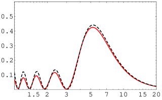
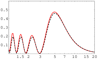
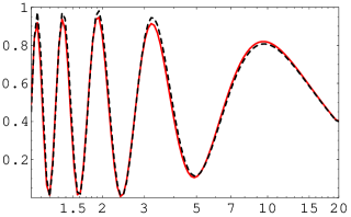
$P(\nu_{e}\to\nu_{e})$	$P(\nu_{\mu}\to\nu_{\mu})$	$P(\nu_{\tau}\to\nu_{\tau})$

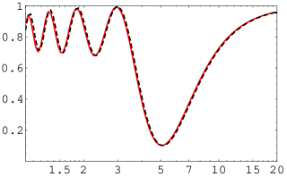
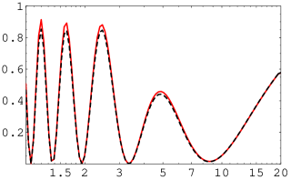
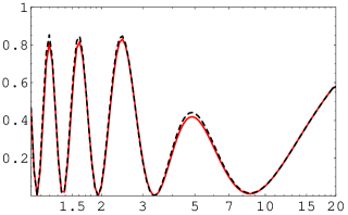
Figure 3: Comparison of our approximate formulas with the numerical calculation. In these figures $P(\nu_{\alpha}\to\nu_{\beta})$ is plotted in order to compare our approximate formulas with the numerical calculation. The solid lines show the approximate probabilities and the dashed lines show the numerical calculation of probabilities.

We compare our approximate formulas with the numerical calculation in figure 3. One can see some features from this figure. The approximated value of probabilities for $P(\nu_{e}\to\nu_{\mu}),P(\nu_{e}\to\nu_{\tau})$ and $P(\nu_{e}\to\nu_{e})$ coincide to the numerical values very well, on the other hand, the remaining three channels of probabilities $P(\nu_{\mu}\to\nu_{\tau}),P(\nu_{\mu}\to\nu_{\mu})$ and $P(\nu_{\tau}\to\nu_{\tau})$ show a small difference between the approximate and the numerical value. However, the difference is not so large as in figure 2 and as a first step the result is sufficiently accurate.

5 Comparison of Our Results with Second Order Formulas

In this section, we concretely calculate the amplitudes by using the approximate formulas derived in the previous section for the case of constant matter and show that simple approximate formulas can be obtained. Finally, we demonstrate that the approximate formula derived with double expansion up to the second order of the two small parameters (second order formulas) are largely different from the exact values in the MSW resonance region under the condition that the baseline length is longer than the oscillation length.

5.1 Approximate Formulas for Amplitudes

In the previous section, we have given a method for approximation of the probabilities in three generations by amplitudes in two generations. In this subsection, we use the constant matter density profile in order to compare our method with other method and investigate the non-perturbative effects. As seen from (4.13)-(4.20), (4.24), (4.26)-(4.28) and (4.34)-(4.39), we only have to calculate four kinds of amplitudes, namely $S_{\mu e}^{\ell},S_{\mu\mu}^{\ell},S_{\tau e}^{h}$ and $S_{\tau\tau}^{h}$.

The low-energy approximate formulas are obtained by taking the limit $s_{13}=0$ and from

$$H^{\ell} = O_{12}{\rm diag}(0,\Delta_{21},\Delta_{31})O_{12}^{T}+{\rm diag}(a,0,0)$$ (5.1)

$$= O^{\ell}_{12}{\rm diag}(\lambda_{1}^{\ell},\lambda_{2}^{\ell},\Delta_{31})(O_{12}^{\ell})^{T}.$$ (5.2)

The effective masses $\lambda_{i}^{\ell}(i=1,2)$ and the effective mixing angle $\theta_{12}^{\ell}$ are determined by the diagonalization of (5.1) to (5.2). If we define the mass squared difference in matter as $\Delta_{21}^{\ell}=\lambda_{2}^{\ell}-\lambda_{1}^{\ell}$, we obtain the relation

$$\frac{\Delta^{\ell}_{21}}{\Delta_{21}}=\frac{\sin 2\theta_{12}}{\sin 2\theta^{\ell}_{12}}=\sqrt{\left(\cos 2\theta_{12}-\frac{a}{\Delta_{21}}\right)^{2}+\sin^{2}2\theta_{12}}.$$ (5.3)

Therefore, the amplitude is calculated as

$$S^{\ell}_{\mu e} = -i\sin 2\theta^{\ell}_{12}\sin\frac{\Delta^{\ell}_{21}L}{2}\exp\left(-i\frac{\Delta_{21}+a}{2}L\right)$$ (5.4)

$$S^{\ell}_{\mu\mu} = \left(\cos\frac{\Delta^{\ell}_{21}L}{2}-i\cos 2\theta^{\ell}_{12}\sin\frac{\Delta^{\ell}_{21}L}{2}\right)\exp\left(-i\frac{\Delta_{21}+a}{2}L\right)$$ (5.5)

by substituting (5.2) into (3.44). On the other hand, the approximate formulas in high energy are obtained by taking the limit $\alpha=0$ and we get

$$H^{h} = O_{13}{\rm diag}(0,0,\Delta_{31})O_{13}^{T}+{\rm diag}(a,0,0)$$ (5.6)

$$= O^{h}_{13}{\rm diag}(\lambda_{1}^{h},0,\lambda_{3}^{h})(O^{h}_{13})^{T}.$$ (5.7)

The effective masses $\lambda_{i}^{h}(i=1,3)$ and the effective mixing angle $\theta_{13}^{h}$ are determined by the diagonalization of (5.6) to (5.7). If we define the mass squared difference in matter as $\Delta_{31}^{h}=\lambda_{3}^{h}-\lambda_{1}^{h}$, we obtain the relation

$$\frac{\Delta^{h}_{31}}{\Delta_{31}}=\frac{\sin 2\theta_{13}}{\sin 2\theta^{h}_{13}}=\sqrt{\left(\cos 2\theta_{13}-\frac{a}{\Delta_{31}}\right)^{2}+\sin^{2}2\theta_{13}}.$$ (5.8)

Accordingly, the amplitude can be calculated by substituting (5.7) into (3.45) as

$$S^{h}_{\tau e} = -i\sin 2\theta^{h}_{13}\sin\frac{\Delta^{h}_{31}L}{2}\exp\left(-i\frac{\Delta_{31}+a}{2}L\right)$$ (5.9)

$$S^{h}_{\tau\tau} = \left(\cos\frac{\Delta^{h}_{31}L}{2}-i\cos 2\theta^{h}_{13}\sin\frac{\Delta^{h}_{31}L}{2}\right)\exp\left(-i\frac{\Delta_{31}+a}{2}L\right).$$ (5.10)

As seen from (5.4) and (5.9), $S_{\mu e}^{\ell}$ and $S_{\tau e}^{h}$ have simple forms, but the expressions of $S_{\mu\mu}^{\ell}$ and $S_{\tau\tau}^{h}$ are more complex than (5.5) and (5.10).

5.2 Approximate Formulas for Probabilities

In this subsection, we derive the approximate formulas of the oscillation probabilities in constant matter by using the result of the previous section.

At first, let us consider the case of including electron neutrino in the initial or final state. In this case, the probability for any channel can be calculated almost in the same way. The probability $P(\nu_{e}\to\nu_{e})$ is obtained by substituting (5.4) and (5.9) into (4.24) as

$$P(\nu_{e}\to\nu_{e})=1-\sin^{2}2\theta^{\ell}_{12}\sin^{2}\frac{\Delta^{\ell}_{21}L}{2}-\sin^{2}2\theta^{h}_{13}\sin^{2}\frac{\Delta^{h}_{31}L}{2}.$$ (5.11)

The probability $P(\nu_{e}\to\nu_{\mu})$ is obtained by substituting (5.4) and (5.9) into (4.14)-(4.16) as

$$P(\nu_{e}\to\nu_{\mu}) = A_{e\mu}\cos\delta+B_{e\mu}\sin\delta+C_{e\mu}$$ (5.12)

$$A_{e\mu} \simeq \sin 2\theta^{\ell}_{12}\sin 2\theta_{23}\sin 2\theta^{h}_{13}\sin\frac{\Delta^{\ell}_{21}L}{2}\sin\frac{\Delta^{h}_{31}L}{2}\cos\frac{\Delta_{32}L}{2}$$ (5.13)

$$B_{e\mu} \simeq \sin 2\theta^{\ell}_{12}\sin 2\theta_{23}\sin 2\theta^{h}_{13}\sin\frac{\Delta^{\ell}_{21}L}{2}\sin\frac{\Delta^{h}_{31}L}{2}\sin\frac{\Delta_{32}L}{2}$$ (5.14)

$$C_{e\mu} \simeq c_{23}^{2}\sin^{2}2\theta^{\ell}_{12}\sin^{2}\frac{\Delta^{\ell}_{21}L}{2}+s_{23}^{2}\sin^{2}2\theta^{h}_{13}\sin^{2}\frac{\Delta^{h}_{31}L}{2}.$$ (5.15)

The remaining probability $P(\nu_{e}\to\nu_{\tau})$ can be calculated from the unitarity relation. Next, let us calculate the probabilities for the case, that not all electron neutrinos in the initial and final state are included. Also in this case, the probability for any channel can be calculated almost in the same way. Accordingly, as an example, we calculate the probability for muon neutrino to tau neutrino,

$$P(\nu_{\mu}\to\nu_{\tau}) = B_{\mu\tau}\sin\delta+C_{\mu\tau}$$ (5.16)

$$B_{\mu\tau} \simeq \sin 2\theta^{\ell}_{12}\sin 2\theta_{23}\sin 2\theta^{h}_{13}\sin\frac{\Delta^{\ell}_{21}L}{2}\sin\frac{\Delta^{h}_{31}L}{2}\sin\frac{\Delta_{32}L}{2}$$ (5.17)

$$C_{\mu\tau} \simeq |S_{\mu\mu}^{\ell}-S_{\tau\tau}^{h}|^{2}s_{23}^{2}c_{23}^{2}.$$ (5.18)

At first, we use the relations, $\cos 2\theta_{12}^{\ell}=2\cos^{2}\theta_{12}^{\ell}-1$ and $\cos 2\theta_{13}^{h}=1-2\sin^{2}\theta_{13}^{h}$, and we rewrite $S_{\mu\mu}^{\ell}$ and $S_{\tau\tau}^{h}$ as

$$S_{\mu\mu}^{\ell} \simeq \left[\exp\left(i\frac{\Delta_{21}^{\ell}}{2}L\right)-2i\cos^{2}\theta^{\ell}_{12}\sin\frac{\Delta^{\ell}_{21}L}{2}\right]\exp\left(-i\frac{\Delta_{21}+a}{2}L\right)$$ (5.19)

$$S_{\tau\tau}^{h} \simeq \left[\exp\left(-i\frac{\Delta^{h}_{31}L}{2}\right)+2i\sin^{2}\theta^{h}_{13}\sin\frac{\Delta^{h}_{31}L}{2}\right]\exp\left(-i\frac{\Delta_{31}+a}{2}L\right).$$ (5.20)

Then, arranging $C_{\mu\tau}$ in the order of the effective mixing angles $\cos\theta_{12}^{\ell}$ and $\sin\theta_{13}^{h}$, we obtain

$$C_{\mu\tau}^{1} = \sin^{2}2\theta_{23}\sin^{2}\frac{(\Delta_{21}^{\ell}+\Delta_{31}^{h}+\Delta_{32})L}{4}$$ (5.21)

$$C_{\mu\tau}^{2a} = -2\sin^{2}2\theta_{23}\cos^{2}\theta_{12}^{\ell}\sin\frac{(\Delta_{21}^{\ell}+\Delta_{31}^{h}+\Delta_{32})L}{4}\cos\frac{(\Delta_{21}^{\ell}-\Delta_{31}^{h}-\Delta_{32})L}{4}\sin\frac{\Delta_{21}^{\ell}L}{2}$$ (5.22)

$$C_{\mu\tau}^{2b} = -2\sin^{2}2\theta_{23}\sin^{2}\theta_{13}^{h}\sin\frac{(\Delta_{21}^{\ell}+\Delta_{31}^{h}+\Delta_{32})L}{4}\cos\frac{(\Delta_{21}^{\ell}-\Delta_{31}^{h}+\Delta_{32})L}{4}\sin\frac{\Delta_{31}^{h}L}{2}$$ (5.23)

$$C_{\mu\tau}^{3} = \sin^{2}2\theta_{23}\cos^{4}\theta^{\ell}_{12}\sin^{2}\frac{\Delta^{\ell}_{21}L}{2}+\sin^{2}2\theta_{23}\sin^{4}\theta_{13}^{h}\sin^{2}\frac{\Delta_{31}^{h}L}{2}$$ (5.24)

$$+ 2\sin^{2}2\theta_{23}\cos^{2}\theta^{\ell}_{12}\sin^{2}\theta^{h}_{13}\sin\frac{\Delta^{\ell}_{21}L}{2}\sin\frac{\Delta^{h}_{31}L}{2}\cos\frac{\Delta_{32}L}{2}.$$

As we show in the following section, the reason of arranging the terms like this is, because the second order formulas can be easily derived. In order to derive the second order formulas, it is sufficient to use $C_{\mu\tau}^{1}$, $C_{\mu\tau}^{2a}$ and $C_{\mu\tau}^{2b}$. We can also calculate the other channels $P(\nu_{\mu}\to\nu_{\mu})$ and $P(\nu_{\tau}\to\nu_{\tau})$ in the same way. In a recent study, it was found that the channels $P(\nu_{\mu}\to\nu_{\mu})$ and $P(\nu_{\tau}\to\nu_{\tau})$ are largely affected by the earth matter in the long baseline [47, 48, 49].

We can see from these expressions that the approximate formulas are rather complex for the case not including electron neutrino in the initial or final state. We also understand from these formulas how matter affects the probabilities. Thus, the formulas are expected to be useful for studying matter effects.

5.3 Large Non-perturbative Effects of small $\alpha$ and $s_{13}$

In this subsection, we compare the approximate formulas obtained in the previous subsection with the second order formulas numerically and it is shown that the latter have a large difference from the numerical value in the MSW resonance region.

The second order formulas are approximated by the main terms of the expansion and are widely used by many authors for their simplicity. In refs. [30, 31], the formula for $P(\nu_{e}\to\nu_{\mu})$ has been derived and later on all probabilities were presented in ref. [32]. As examples, the probabilities, $P(\nu_{e}\to\nu_{\mu})$ and $P(\nu_{\mu}\to\nu_{\tau})$, are taken. For the other channels of probabilities, similar expressions have been obtained. In all channels similar results were obtained from comparison with numerical calculations. The second order formula for $P(\nu_{e}\to\nu_{\mu})$ is given by

$$P(\nu_{e}\to\nu_{\mu}) = A_{e\mu}\cos\delta+B_{e\mu}\sin\delta+C_{e\mu},$$ (5.25)

$$A_{e\mu} \simeq \alpha s_{13}\sin 2\theta_{12}\sin 2\theta_{23}\frac{2\Delta_{31}^{2}}{a(\Delta_{31}-a)}\sin\frac{aL}{2}\sin\frac{(\Delta_{31}-a)L}{2}\cos\frac{\Delta_{32}L}{2}$$ (5.26)

$$B_{e\mu} \simeq \alpha s_{13}\sin 2\theta_{12}\sin 2\theta_{23}\frac{2\Delta_{31}^{2}}{a(\Delta_{31}-a)}\sin\frac{aL}{2}\sin\frac{(\Delta_{31}-a)L}{2}\sin\frac{\Delta_{32}L}{2}$$ (5.27)

$$C_{e\mu} \simeq \alpha^{2}c_{23}^{2}\sin^{2}2\theta_{12}\frac{\Delta_{31}^{2}}{a^{2}}\sin^{2}\frac{aL}{2}+s_{13}^{2}s_{23}^{2}\frac{4\Delta_{31}^{2}}{(\Delta_{31}-a)^{2}}\sin^{2}\frac{(\Delta_{31}-a)L}{2}.$$ (5.28)

Comparing our approximate formulas (5.13)-(5.15) with the second order formulas (5.26)-(5.28), each term corresponds one by one. Actually, the second order formulas (5.26)-(5.28) are derived by expanding our approximate formulas (5.13)-(5.15) up to the second order in $\alpha$ and $s_{13}$ [44]. Next, the second order formula for $P(\nu_{\mu}\to\nu_{\tau})$ which has been already derived in ref. [32] is

$$P(\nu_{\mu}\to\nu_{\tau}) = A_{\mu\tau}\cos\delta+B_{\mu\tau}\sin\delta+C_{\mu\tau}$$ (5.29)

$$A_{\mu\tau} \simeq \alpha s_{13}\sin^{2}2\theta_{23}\sin 2\theta_{12}\cos 2\theta_{23}\frac{2\Delta_{31}}{\Delta_{31}-a}\sin\frac{\Delta_{31}L}{2}$$ (5.30)

$$\times \left[\frac{a}{\Delta_{31}}\sin\frac{\Delta_{31}L}{2}-\frac{\Delta_{31}}{a}\sin\frac{aL}{2}\cos\frac{(\Delta_{31}-a)L}{2}\right]$$

$$B_{\mu\tau} \simeq \alpha s_{13}\sin 2\theta_{12}\sin 2\theta_{23}\frac{2\Delta_{31}^{2}}{a(\Delta_{31}-a)}\sin\frac{aL}{2}\sin\frac{(\Delta_{31}-a)L}{2}\sin\frac{\Delta_{32}L}{2},$$ (5.31)

and $C_{\mu\tau}$ is given by

$$C_{\mu\tau} \simeq \sin^{2}2\theta_{23}\sin^{2}\frac{\Delta_{31}L}{2}$$ (5.32)

$$- \alpha\sin^{2}2\theta_{23}\cos^{2}\theta_{12}\left(\frac{\Delta_{31}L}{2}\right)\sin\Delta_{31}L+\alpha^{2}\sin^{2}2\theta_{23}\cos^{4}\theta_{12}\left(\frac{\Delta_{31}L}{2}\right)^{2}\cos\Delta_{31}L$$

$$- \alpha^{2}\sin^{2}2\theta_{23}\sin^{2}2\theta_{12}\left(\frac{\Delta_{31}}{2a}\right)\left[\sin\frac{\Delta_{31}L}{2}\cos\frac{(\Delta_{31}-a)L}{2}\sin\frac{aL}{2}\left(\frac{\Delta_{31}}{a}\right)-\frac{\Delta_{31}L}{4}\sin(\Delta_{31}L)\right]$$

$$- s_{13}^{2}\sin^{2}2\theta_{23}\frac{2\Delta_{31}}{\Delta_{31}-a}\left[\sin\frac{\Delta_{31}L}{2}\cos\frac{aL}{2}\sin\frac{(\Delta_{31}-a)L}{2}\left(\frac{\Delta_{31}}{\Delta_{31}-a}\right)-\frac{aL}{4}\sin(\Delta_{31}L)\right].$$

In the next section we show that this formula (5.32) can be also derived from our formulas (5.21)-(5.24). It is noted that the second order formula (5.32) for $C_{\mu\tau}$ is rather complex. Furthermore comparing our approximate formula (5.17)-(5.24) with the second order formula (5.30)-(5.32), we see that $A_{\mu\tau}$ is not included in our formula. The reason is, that $A_{\mu\tau}=0$ in the case of maximal mixing angle $\sin 2\theta_{23}=1$ and there is no way of calculating this by the method described in this paper. If we consider $\cos 2\theta_{23}$ as a small parameter like $\alpha$ and $s_{13}$, this $A_{\mu\tau}$ has the magnitude of $O(\alpha s_{13}\cos 2\theta_{23})$. Therefore, $A_{\mu\tau}$ is proportional to the third order of small parameters and is expected to be neglectable. This means that our formula is not largely affected by the error due to this term, which cannot be derived from our method. However, as this error affects the precision measurement of $\sin\theta_{23}$ by the atmospheric neutrino experiments in future, the improvement of this point is important future work. The formulas for the other channels are given in ref. [32]. The second order formulas are effective under the following two conditions.

The first one is for the neutrino energy and is given by

$$E\gg 0.45\>{\rm GeV}\left(\frac{\Delta m_{21}^{2}}{10^{-4}\>{\rm eV^{2}}}\right)\left(\frac{3\>{\rm g/cm^{3}}}{\rho}\right).$$ (5.33)

The second one is for the baseline length and is given by

$$L\ll 8000\>{\rm km}\left(\frac{E}{{\rm GeV}}\right)\left(\frac{10^{-4}\>{\rm eV^{2}}}{\Delta m_{21}^{2}}\right).$$ (5.34)

These conditions come from the utilization of perturbative expansion on the two small parameters. The detailed discussion are given in [31]. These approximate formulas are used for the purpose of understanding of the results obtained by numerical calculations [50, 51]. However, as shown in the next figure, these formulas have large difference from the true value in the MSW resonance region, which is considered to be the most important region.

Next, let us compare our formulas (5.12)-(5.23) with the second order formulas (5.25)-(5.32) in all channels by numerical calculation. In order to see the magnitude of the error, we also compare two kinds of approximate formulas with the exact values. We set the baseline length as $L=6000~{}{\rm km}$, where the MSW effect becomes large, and the energy region as $1~{}{\rm GeV}\leq E\leq 20~{}{\rm GeV}$, where the MSW resonance energy is included. Furthermore, the second order formulas are derived only in the case of constant matter, so we choose the average density $\rho=3.91~{}{\rm g/cm^{3}}$ of the earth calculated by the PREM. Note that two conditions (5.33) and (5.34) are satisfied in these region.

$P(\nu_{e}\to\nu_{\mu})$	$P(\nu_{e}\to\nu_{\tau})$	$P(\nu_{\mu}\to\nu_{\tau})$
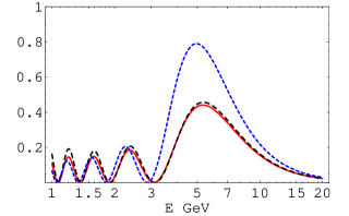
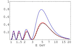
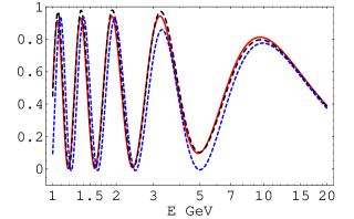
$P(\nu_{e}\to\nu_{e})$	$P(\nu_{\mu}\to\nu_{\mu})$	$P(\nu_{\tau}\to\nu_{\tau})$

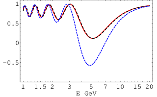
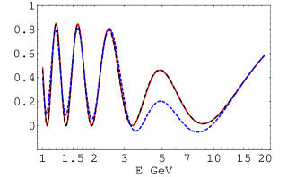
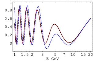
Figure 4: Comparison of our approximate formulas with the second order formulas and in addition with the numerical calculations. The solid, dashed and dotted lines show the probabilities in our approximate formulas, those in the numerical calculation and those in the second order formulas, respectively.

We compare the probabilities calculated by our approximate formulas in all channels with those by the second order formulas in addition to numerical calculation in figure 4. One can see the following points from this figure. The second order formulas show large differences from the numerical values around 5 GeV, where the high energy MSW resonance occurs. In other energy regions they are in good coincidence. The value of $P(\nu_{e}\to\nu_{e})$ has the largest difference, the probabilities $P(\nu_{e}\to\nu_{\mu})$ and $P(\nu_{e}\to\nu_{\tau})$ have the next largest difference, the values of $P(\nu_{\mu}\to\nu_{\mu})$ and $P(\nu_{\tau}\to\nu_{\tau})$ have also significantly large difference, but only the probability $P(\nu_{\mu}\to\nu_{\tau})$ has a small difference. In addition, these figures show that the difference between the second order formulas and the numerical calculation exists even in the two applicable regions (5.33) and (5.34). Although we do not show a figure, the difference between our approximate formulas (5.12)-(5.23) and the second order formulas (5.25)-(5.32) become more clear out of the two applicable regions (5.33) and (5.34). The reason is that our approximate formulas (5.12)-(5.23) are applicable even for the case that the condition (5.33) or (5.34) for energy and baseline length does not hold, as confirmed from the comparison with the exact numerical calculation. However, the second order formulas are good approximations, when the neutrino energy is not near the resonance energy, even if the baseline length is long.

6 Non-perturbative Effects of Small Parameters $\Delta m_{21}^{2}/\Delta m_{31}^{2}$ and $\sin\theta_{13}$

In this section, we investigate the reason for the difference between the second order formula,which contains the approximation with double expansion up to the second order of two small parameters, and the numerical calculation around the MSW resonance region as explained in the previous subsection.

We discuss the non-perturbative effects of small mixing angle more detailed than in section 2.

6.1 Derivation of the Second Order Formulas

In this subsection, we investigate how the second order formulas are approximated expanding on $\alpha=\Delta m_{21}^{2}/\Delta m_{31}^{2}$ In the previous paper, we have discussed the probability $P(\nu_{e}\to\nu_{\mu})$, so we calculate the second order formula for $P(\nu_{\mu}\to\nu_{\tau})$ here. The method of calculation is basically the same but the calculation itself becomes slightly complex, because we need to calculate the effective mass and the effective mixing angle up to the second order of $\alpha$ and $s_{13}$ in the case of $P(\nu_{\mu}\to\nu_{\tau})$. In this point, the calculation is not straightforward compared with that of $P(\nu_{e}\to\nu_{\mu})$ but the method of approximation is the same. Note that $C_{\mu\tau}^{1}$ in (5.21) does not include the effective mixing angle. For this reason, it is sufficient to expand the effective mixing angle up to the zeroth order, but we need to expand the effective mass up to the second order to calculate the probability up to the second order in $\alpha$ and $s_{13}$, The effective mixing angle is expanded up to the zeroth order as

$$\cos\theta_{12}^{\ell} \simeq \frac{1}{2}\sin 2\theta_{12}^{\ell}\simeq\alpha\sin 2\theta_{12}\frac{\Delta_{31}}{2a}$$ (6.1)

$$\sin\theta_{13}^{h} \simeq \frac{1}{2}\sin 2\theta_{13}^{h}\simeq s_{13}\frac{\Delta_{31}}{\Delta_{31}-a}$$ (6.2)

and the effective mass is expanded up to the second order as

$$\Delta^{\ell}_{21} \simeq a-\alpha\cos 2\theta_{12}\Delta_{31}+\alpha^{2}\sin^{2}2\theta_{12}\frac{\Delta_{31}^{2}}{2a}$$ (6.3)

$$\Delta^{h}_{31} \simeq \Delta_{31}-a+s_{13}^{2}\frac{2\Delta_{31}a}{\Delta_{31}-a}.$$ (6.4)

Here, we should emphasize the following points. Eqs. (6.1) and (6.3) obtained by the expansion in $\alpha$ diverge in the vacuum limit $a\to 0$ and eqs. (6.2) and (6.4) obtained by the expansion in $s_{13}$ diverge in the high energy MSW resonance limit $a\to\Delta_{31}$. As shown in the following, these divergences cancel and the probability has a finite value. Expanding $C_{\mu\tau}^{1}$ in (5.21) up to the second order, we obtain

$$C_{\mu\tau}^{1} \simeq C_{\mu\tau}^{1a}+C_{\mu\tau}^{1b}+C_{\mu\tau}^{1c}+C_{\mu\tau}^{1d}+C_{\mu\tau}^{1e}$$ (6.5)

$$C_{\mu\tau}^{1a} = \sin^{2}2\theta_{23}\sin^{2}\frac{\Delta_{31}L}{2}$$ (6.6)

$$C_{\mu\tau}^{1b} = -\alpha\sin^{2}2\theta_{23}\cos^{2}\theta_{12}\left(\frac{\Delta_{31}L}{2}\right)\sin\Delta_{31}L$$ (6.7)

$$C_{\mu\tau}^{1c} = \alpha^{2}\sin^{2}2\theta_{23}\cos^{4}\theta_{12}\left(\frac{\Delta_{31}L}{2}\right)^{2}\cos\Delta_{31}L$$ (6.8)

$$C_{\mu\tau}^{1d} = \alpha^{2}\sin^{2}2\theta_{23}\sin^{2}2\theta_{12}\left(\frac{\Delta_{31}^{2}L}{8a}\right)\sin\Delta_{31}L$$ (6.9)

$$C_{\mu\tau}^{1e} = s_{13}^{2}\sin^{2}2\theta_{23}\left(\frac{a\Delta_{31}}{\Delta_{31}-a}\frac{L}{2}\right)\sin\Delta_{31}L.$$ (6.10)

We also expand $C_{\mu\tau}^{2a}$ in (5.22) and $C_{\mu\tau}^{2b}$ in (5.23) as

$$C_{\mu\tau}^{2a} \simeq -2\alpha^{2}\sin^{2}2\theta_{23}\sin^{2}2\theta_{12}\left(\frac{\Delta_{31}}{2a}\right)^{2}\sin\frac{\Delta_{31}L}{2}\cos\frac{(\Delta_{31}-a)L}{2}\sin\frac{aL}{2}$$ (6.11)

$$C_{\mu\tau}^{2b} \simeq -2s_{13}^{2}\sin^{2}2\theta_{23}\left(\frac{\Delta_{31}}{\Delta_{31}-a}\right)^{2}\sin\frac{\Delta_{31}L}{2}\cos\frac{aL}{2}\sin\frac{(\Delta_{31}-a)L}{2}.$$ (6.12)

Finally, we obtain (5.32) arranging these result order by order.

Here, let us consider the applicable region of the second order formulas. $C_{\mu\tau}^{1d}$ diverges in the limit $a\to 0$ and $C_{\mu\tau}^{1e}$ diverges in the limit $a\to\Delta_{31}$. $C_{\mu\tau}^{2a}$ also diverges in the limit $a\to 0$ and $C_{\mu\tau}^{2b}$ diverges in the limit $a\to\Delta_{31}$. The divergences in $a\to 0$ and in $a\to\Delta_{31}$ come from the expansion of the effective masses (6.3) and (6.4) respectively. It seems that the second order formulas do not reduce to those in vacuum due to the divergence in $a\to 0$ and furthermore do not reduce to those in the high energy MSW resonance point due to the divergence in $a\to\Delta_{31}$. However, when we consider the pair

$$C_{\mu\tau}^{1d}+C_{\mu\tau}^{2a}=-\alpha^{2}\sin^{2}2\theta_{23}\sin^{2}2\theta_{12}\frac{\Delta_{31}}{2a}\left[\sin\frac{\Delta_{31}L}{2}\cos\frac{(\Delta_{31}-a)L}{2}\sin\frac{aL}{2}\left(\frac{\Delta_{31}}{a}\right)-\frac{\Delta_{31}L}{4}\sin(\Delta_{31}L)\right],$$ (6.13)

the divergence in $a\to 0$ cancel and the value converges. The obtained finite value is given by

$$\lim_{a\to 0}(C_{\mu\tau}^{1d}+C_{\mu\tau}^{2a})=-\alpha^{2}\sin^{2}2\theta_{23}\sin^{2}2\theta_{12}\frac{1}{2}\left(\frac{\Delta_{31}L}{2}\right)^{2}\sin^{2}\frac{\Delta_{31}L}{2}.$$ (6.14)

Before we expand, $C_{\mu\tau}^{1}$ and $C_{\mu\tau}^{2}$ have finite values in the limit $a\to 0$ and $a\to\Delta_{31}$. However, the divergence appears in expansion of $\alpha$ and $s_{13}$. The cancellation of these divergences occurs between $C_{\mu\tau}^{1d}$ and $C_{\mu\tau}^{2a}$. This means that the cancellation occurs between the different terms and result in finite values, respectively, at first, which is an interesting result. Considering the pair as

$$C_{\mu\tau}^{1e}+C_{\mu\tau}^{2b}=-s_{13}^{2}\sin^{2}2\theta_{23}\frac{2\Delta_{31}}{\Delta_{31}-a}\left[\sin\frac{\Delta_{31}L}{2}\cos\frac{aL}{2}\sin\frac{(\Delta_{31}-a)L}{2}\left(\frac{\Delta_{31}}{\Delta_{31}-a}\right)-\frac{aL}{4}\sin(\Delta_{31}L)\right],$$ (6.15)

the divergence in the limit $a\to\Delta_{31}$ cancels and the value converges. The finite value is given by

$$\lim_{a\to\Delta_{31}}(C_{\mu\tau}^{1e}+C_{\mu\tau}^{2b})=s_{13}^{2}\sin^{2}2\theta_{23}\left(\frac{\Delta_{31}L}{2}\right)\left[(\Delta_{31}L)\sin^{2}\frac{\Delta_{31}L}{2}-\sin(\Delta_{31}L)\right].$$ (6.16)

The cancellation of these divergences occurs between the different terms $C_{\mu\tau}^{1e}$ and $C_{\mu\tau}^{2b}$, which is also a remarkable result.

We have shown that the second order formulas have finite values in the limit $a\to 0$ and $a\to\Delta_{31}$, but it is not always the same as that in the numerical calculation. Actually, the difference in fig. 4 in the limit $a\to\Delta_{31}$, shows that the second order formulas have finite values but they are not in accordance with those in the numerical calculation. In order to study this, we compare the three quantities, the numerical calculation, our formulas and the second order formulas. We can learn the differences mainly in the vacuum limit $a\to 0$ and the high energy MSW resonance limit $a\to\Delta_{31}$ from the comparison.

At first, let us consider the vacuum limit $a\to 0$. Furthermore, to simplify the discussion, we consider the case of $s_{13}\to 0$. The second order formulas in the limits $a\to 0$ and $s_{13}\to 0$ are given by

$$\lim_{a,s_{13}\to 0}C_{\mu\tau}^{\rm(double)} = \sin^{2}2\theta_{23}\sin^{2}\frac{\Delta_{31}L}{2}-\alpha\sin^{2}2\theta_{23}\cos^{2}\theta_{12}\left(\frac{\Delta_{31}L}{2}\right)\sin\Delta_{31}L$$ (6.17)

$$+ \alpha^{2}\sin^{2}2\theta_{23}\cos^{4}\theta_{12}\left(\frac{\Delta_{31}L}{2}\right)^{2}\cos\Delta_{31}L$$

$$- \alpha^{2}\sin^{2}2\theta_{23}\sin^{2}2\theta_{12}\frac{1}{2}\left(\frac{\Delta_{31}L}{2}\right)^{2}\sin^{2}\frac{\Delta_{31}L}{2}.$$

Next, taking the limit $a\to 0$ and $s_{13}\to 0$ in our formulas, we obtain

$$\lim_{a,s_{13}\to 0}C_{\mu\tau}^{\rm(exact)} = \sin^{2}2\theta_{23}\sin^{2}\frac{\Delta_{31}L}{2}$$ (6.18)

$$- 2\sin^{2}2\theta_{23}\cos^{2}\theta_{12}\sin\frac{\Delta_{31}L}{2}\cos\frac{(\Delta_{21}-\Delta_{31})L}{2}\sin\frac{\Delta_{21}L}{2}.$$

Expanding the oscillating part of (6.18) in our formula, it leads to (6.17) obtained from the second order formula. The condition for the expansion on the oscillating part for sufficiently good approximation is

$$L<\frac{2}{\Delta_{21}}.$$ (6.19)

Next, let us consider the high energy MSW resonance limit $a\to\Delta_{31}$. In order to simplify the discussion, we take the high energy MSW resonance limit $a\to\Delta_{31}$ under the condition $\alpha\to 0$. In the high energy MSW resonance limit of the second order formula, we obtain

$$\lim_{a\to\Delta_{31},\alpha\to 0}C_{\mu\tau}^{\rm(double)} = \sin^{2}2\theta_{23}\sin^{2}\frac{\Delta_{31}L}{2}$$ (6.20)

$$+ s_{13}^{2}\sin^{2}2\theta_{23}\left(\frac{\Delta_{31}L}{2}\right)\left[(\Delta_{31}L)\sin^{2}\frac{\Delta_{31}L}{2}-\sin(\Delta_{31}L)\right].$$

Next, taking the limit $a\to\Delta_{31}$ and $\alpha\to 0$ in our formulas, we obtain

$$\lim_{a\to\Delta_{31},\alpha\to 0}C_{\mu\tau}^{\rm(exact)} = \sin^{2}2\theta_{23}\sin^{2}\frac{(1+s_{13})\Delta_{31}L}{2}$$ (6.21)

$$- \sin^{2}2\theta_{23}(1-s_{13}^{2})\sin\frac{(1+s_{13})\Delta_{31}L}{2}\cos\frac{(1-s_{13})\Delta_{31}L}{4}\sin(s_{13}\Delta_{31}L).$$

By expanding the oscillating part obtained from our formula (6.21), it is shown that this coincides with that from the second order formula (6.20). The condition for the expansion of the oscillating part for a sufficient approximation is given by

$$L<\frac{2}{s_{13}\Delta_{31}}=\frac{2}{s_{13}a}.$$ (6.22)

If the baseline length is shorter than that obtained from above condition, the second order formula becomes a good approximation. We obtain the following results about the perturbative expansion on the small parameters $\alpha$ and $s_{13}$.

1. The perturbative expansion in $\alpha$ actually corresponds to the expansion in $\Delta_{21}/a$. This constrains the applicable energy for the approximate formulas. If we expand in the parameter $\Delta_{21}/a$, the effective mass $\Delta^{\ell}_{21}$ and the effective mixing angle $\sin 2\theta^{\ell}_{12}$ diverge in the vacuum limit $a\to 0$. However, these divergences cancel out each other in the calculation of the oscillation probability. Thus, the probability has a finite value, but the value largely differs from the numerical calculation in low-energy. The magnitude of this difference becomes large and serious in the case of small mixing angles and in low-energy long baseline experiments.

2. If we expand in the small mixing angle $s_{13}$, the effective mass $\Delta^{h}_{31}$ and the effective mixing angle $\sin 2\theta^{h}_{13}$ diverge in the MSW resonance energy limit $a\to\Delta_{31}$. However, these divergences also cancel each other out in the calculation of the oscillation probability. Thus, the probability has a finite value, but the value largely differs from the numerical calculation in the high-energy MSW resonance region. This means that the second order formulas cannot be used in the high energy MSW resonance region.

In two generations, we can calculate the oscillation probabilities exactly by solving the second order equation. So, we do not need the perturbative expansion. On the other hand, the construction of the approximate formulas applicable to arbitrary matter density profile is very difficult in three generations. Therefore, we need to expand on the small parameters $\alpha$ and $s_{13}$.

6.2 Discussion

We have shown that the double expansion formulas up to the second order in the two small parameters $\alpha$ and $s_{13}$ does not give a good approximation in the MSW resonance region. This is because the coefficients of the small parameters have large values in the MSW resonance region. In this subsection, let us discuss some methods proposed up to present to solve this problem. The Hamiltonian $H^{\prime}$ is written by four parameters. The two parameters $(\Delta m^{2}_{21},\theta_{12})$ control the physics mainly in the low-energy region and the other two parameters $(\Delta m^{2}_{31},\theta_{13})$ control the physics mainly in the high-energy region. In other words, the magnitude of $\alpha$ determines low-energy phenomena and the magnitude of $s_{13}$ determines high-energy phenomena. Both of these parameters are very small but the energy region, where the expansion converges, is different. This means that we need to treat the applicable energy region carefully when we expand on these two parameters. There are several methods in order to take into account the higher order terms of $\alpha$ and $s_{13}$ for example

1. exact formulas in constant matter density profile

2. reduction formulas taking into account the two generation part exactly

In the first method, there does not exist any error generated from the perturbative expansion, because of the exact treatment of both $\alpha$ and $s_{13}$ [42]. Furthermore, non-perturbative effects can be easily investigated by using these exact formulas. The second method was introduced in our previous paper [44]. In this method, we try to include the higher order terms of $\alpha$ and $s_{13}$ partially, except for the terms including the product of two small parameters. This method includes the higher order terms of $\alpha$ and $s_{13}$ and is simply and applicable even in the case of arbitrary matter density profile [44, 45]. Although this method uses only the second order approximation of the amplitude, it has the notable feature that the third order (three generation) effects such as CP violation can be calculated.

7 Summary

In this paper, we consider the method how to approximates the neutrino oscillation probabilities in matter under three generations and the obtained results are summarized as following.

1. In the framework of two generation neutrino oscillation, we discuss the applicable region of the perturbative expansion on the small mixing angle in matter. The result of the perturbation differs largely from the exact numerical calculation in the MSW resonance point. This means that non-perturbative effects are important even for the neutrino oscillation in two generations.

2. We extend the method [44, 45] to calculate the approximate formulas, in which non-perturbative effects of the small parameters $\Delta m_{21}^{2}/\Delta m_{31}^{2}$ and $\sin\theta_{13}$, to all channels. Under the conditions, $\theta_{23}=45^{\circ}$ and the symmetric matter density profile, we derive simple approximate formulas of the probabilities in all channels by using the unitary relation. Although all these approximate formulas are expressed by the amplitudes calculated within the framework of two generations, it has a notable feature that the three generation effects such as CP violation can also be calculated.

3. In the three generation neutrino oscillation with matter, we investigate non-perturbative effects of the two small parameters $\Delta m_{21}^{2}/\Delta m_{31}^{2}$ and $\sin\theta_{13}$. We compare our approximate formulas with those from the double expansion, which include the terms up to the second order in the low and high energy MSW resonance regions. The obtained result is that the second order formulas show large differences from the exact numerical calculation, which means that non-perturbative effects of the small $\Delta m_{21}^{2}/\Delta m_{31}^{2}$ and $\sin\theta_{13}$ become important in the MSW resonance region.

Finally, we describe two problems that we could not fully address in this paper, and which are tasks for future research.

1. The approximate formulas in this paper are derived by using the condition $\theta_{23}=45^{\circ}$, which is the center value obtained from the atmospheric neutrino experiments. However, but differences from this value may exist within 90% confidence level.

2. The condition for the symmetric matter density is satisfied in the 1-dimensional models, like the PREM and the ak135f, but the actual matter density, for example, that from J-PARC to Beijing is not symmetric [52]. Therefore, our aim for future work is, to derive more sophisticated approximate formulas that hold not only in symmetric matter but in arbitrary matter as well.

To solve the above two problems are the future works This is now included in the upper sentence.

Appendix A General Feature of CP Dependence

In this appendix we calculate the coefficients of the probabilities in detail. We show that the 2-3 mixing angle and the CP phase are not affected by matter, from a different point of view as described in our previous paper [41]. This result means that we only have to consider the matter effects on four parameters $(\Delta m_{21}^{2},\theta_{12})$ and $(\Delta m_{31}^{2},\theta_{13})$. By using this result, we can understand the matter effects in three generations, which become complex compared with that in two generations.

A.1 Remarkable Features of Effective Masses

In this subsection, we show that $(\theta_{23},\delta)$ do not affect the effective mass in three generation Hamiltonian. If we express the effective Hamiltonian in matter as

$$H=U{\rm diag}(0,\Delta_{21},\Delta_{31})U^{\dagger}+{\rm diag}(a,0,0),$$ (A.1)

the equation of eigenvalue is given by

$${\rm det}(t-H) = t^{3}-(\Delta_{21}+\Delta_{31}+a)t^{2}$$ (A.2)

$$+ (\Delta_{21}\Delta_{31}+a(\Delta_{21}(1-|U_{e2}|^{2})+\Delta_{31}(1-|U_{e3}|^{2})))t-a\Delta_{21}\Delta_{31}|U_{e1}|^{2}=0,$$

and by solving this equation, we obtain the effective masses as

$$\lambda_{1} = \frac{A}{3}-\frac{1}{3}\sqrt{A^{2}-3B}S-\frac{\sqrt{3}}{3}\sqrt{A^{2}-3B}\sqrt{1-S^{2}}$$ (A.3)

$$\lambda_{2} = \frac{A}{3}-\frac{1}{3}\sqrt{A^{2}-3B}S+\frac{\sqrt{3}}{3}\sqrt{A^{2}-3B}\sqrt{1-S^{2}}$$ (A.4)

$$\lambda_{3} = \frac{A}{3}+\frac{2}{3}\sqrt{A^{2}-3B}S$$ (A.5)

[46], where $A,B,C$ and $S$ are defined by

$$A = \Delta_{21}+\Delta_{31}+a$$ (A.6)

$$B = \Delta_{21}\Delta_{31}+a[\Delta_{21}(1-|U_{e2}|^{2})+\Delta_{31}(1-|U_{e3}|^{2})]$$ (A.7)

$$C = a\Delta_{21}\Delta_{31}|U_{e1}|^{2}$$ (A.8)

$$S = \cos\left[\frac{1}{3}\arccos\left(\frac{2A^{3}-9AB+27C}{2\sqrt{(A^{2}-3B)^{3}}}\right)\right].$$ (A.9)

These effective masses depend only on the following three vacuum mixing angles

$$|U_{e1}|=c_{12}c_{13},\quad|U_{e2}|=s_{12}c_{13},\quad|U_{e3}|=s_{13}.$$ (A.10)

One can see from these equalities that the effective masses are independent of the 2-3 mixing angle $\theta_{23}$ and the CP phase $\delta$. Next, let us consider this result from a different point of view.

A.2 Decomposition of 2-3 mixing and CP Phase from Hamiltonian

In this section, we separate $\theta_{23}$ and $\delta$ from the Hamiltonian and we study the dependence of the amplitudes on the two small parameters $\alpha$ and $s_{13}$. The Standard Parametrization is defined by

$$U=O_{23}\Gamma O_{13}\Gamma^{\dagger}O_{12},$$ (A.11)

where the CP phase matrix $\Gamma$ is given by

$$\Gamma={\rm diag}(1,1,e^{i\delta}).$$ (A.12)

The CP phase matrix $\Gamma$ and the 1-2 mixing matrix $O_{12}$ are commutable as

$$[\Gamma,O_{12}]=[\Gamma,{\rm diag}(0,\Delta_{21},\Delta_{31})]=0.$$ (A.13)

Therefore, the Hamiltonian can be separated as

$$H(t)=U{\rm diag}(0,\Delta_{21},\Delta_{31})U^{\dagger}+{\rm diag}(a(t),0,0)=O_{23}\Gamma H^{\prime}(t)\Gamma^{\dagger}O_{23}^{T},$$ (A.14)

where $H^{\prime}(t)$ is defined by

$$H^{\prime}(t)=O_{13}O_{12}{\rm diag}(0,\Delta_{21},\Delta_{31})O_{12}^{T}O_{13}^{T}+{\rm diag}(a(t),0,0).$$ (A.15)

This means that the 2-3 mixing and the CP phase can be separated from the part which includes the matter effects $a(t)$.

In the case of constant matter density profile, we obtain

$${\rm det}(\lambda-H)={\rm det}(\lambda-H^{\prime}),$$ (A.16)

the 2-3 mixing angle and the CP phase do not affect the eigenvalue equation. Accordingly, the effective masses are independent of the 2-3 mixing angle and the CP phase, which coincide with the result obtained in the previous subsection.

A.3 Exact CP and 2-3 mixing Dependence of Oscillation Probabilities

Here, let us consider the case in which we apply the above discussion used in the Hamiltonian to the amplitude. Solving the Schrodinger eq. for the amplitude in matter, we obtain

$$S(t)={\rm T}\exp\left\{-i\int H(t)dt\right\}.$$ (A.17)

By using this, we obtain

$$S(t)={\rm T}\exp\left\{-i\int O_{23}\Gamma H^{\prime}(t)\Gamma^{\dagger}O_{23}^{T}dt\right\}=O_{23}\Gamma{\rm T}\exp\left\{-i\int H^{\prime}(t)dt\right\}\Gamma^{\dagger}O_{23}^{T}=O_{23}\Gamma S^{\prime}(t)\Gamma^{\dagger}O_{23}^{T}$$ (A.18)

from (A.14). Therefore, $S(t)$ satisfies

$$S(t)=O_{23}\Gamma S^{\prime}(t)\Gamma^{\dagger}O_{23}^{T}.$$ (A.19)

From this equation, we obtain

$$P(\nu_{e}\to\nu_{e}) = C_{ee},$$ (A.20)

$$P(\nu_{\alpha}\to\nu_{\beta}) = A_{\alpha\beta}\cos\delta+B_{\alpha\beta}\sin\delta+C_{\alpha\beta},$$ (A.21)

when the initial or final state is $\nu_{e}$, and

$$P(\nu_{\alpha}\to\nu_{\beta}) = A_{\alpha\beta}\cos\delta+B_{\alpha\beta}\sin\delta+C_{\alpha\beta}+D_{\alpha\beta}\cos 2\delta+E_{\alpha\beta}\sin 2\delta,$$ (A.22)

in the case of $\nu_{\alpha},\nu_{\beta}=\nu_{\mu},\nu_{\tau}$ [41]. The final result is given by

$$P(\nu_{e}\to\nu_{e}) = C_{ee}=|S^{\prime}_{ee}|^{2},$$ (A.23)

$$P(\nu_{e}\to\nu_{\mu}) = A_{e\mu}\cos\delta+B_{e\mu}\sin\delta+C_{e\mu},$$ (A.24)

$$A_{e\mu} = 2{\rm Re}[{S}_{\mu e}^{{}^{\prime}*}S^{\prime}_{\tau e}]c_{23}s_{23},\hskip 5.0pt$$ (A.25)

$$B_{e\mu} = -2{\rm Im}[{S}_{\mu e}^{{}^{\prime}*}S^{\prime}_{\tau e}]c_{23}s_{23},\hskip 5.0pt$$ (A.26)

$$C_{e\mu} = |S^{\prime}_{\mu e}|^{2}c_{23}^{2}+|S^{\prime}_{\tau e}|^{2}s_{23}^{2},\hskip 5.0pt$$ (A.27)

$$P(\nu_{e}\to\nu_{\tau}) = A_{e\tau}\cos\delta+B_{e\tau}\sin\delta+C_{e\tau},$$ (A.28)

$$A_{e\tau} = -2{\rm Re}[{S}_{\mu e}^{{}^{\prime}*}S^{\prime}_{\tau e}]c_{23}s_{23},\hskip 5.0pt$$ (A.29)

$$B_{e\tau} = 2{\rm Im}[{S}_{\mu e}^{{}^{\prime}*}S^{\prime}_{\tau e}]c_{23}s_{23},\hskip 5.0pt$$ (A.30)

$$C_{e\tau} = |S^{\prime}_{\mu e}|^{2}s_{23}^{2}+|S^{\prime}_{\tau e}|^{2}c_{23}^{2},\hskip 5.0pt$$ (A.31)

$$P(\nu_{\mu}\to\nu_{\mu}) = A_{\mu\mu}\cos\delta+B_{\mu\mu}\sin\delta+C_{\mu\mu}+D_{\mu\mu}\cos 2\delta+E_{\mu\mu}\sin 2\delta,$$ (A.32)

$$A_{\mu\mu} = 2{\rm Re}[({S}^{\prime}_{\mu\mu}c_{23}^{2}+S^{\prime}_{\tau\tau}s_{23}^{2})^{*}({S}^{\prime}_{\tau\mu}+S^{\prime}_{\mu\tau})]c_{23}s_{23},\hskip 5.0pt$$ (A.33)

$$B_{\mu\mu} = -2{\rm Im}[({S}^{\prime}_{\mu\mu}c_{23}^{2}+S^{\prime}_{\tau\tau}s_{23}^{2})^{*}({S}^{\prime}_{\tau\mu}-S^{\prime}_{\mu\tau})]c_{23}s_{23},\hskip 5.0pt$$ (A.34)

$$C_{\mu\mu} = |S^{\prime}_{\mu\mu}|^{2}c_{23}^{4}+|S^{\prime}_{\tau\tau}|^{2}s_{23}^{4}+(|S^{\prime}_{\mu\tau}|^{2}+|S^{\prime}_{\tau\mu}|^{2}+2{\rm Re}[{S}_{\mu\mu}^{{}^{\prime}*}S^{\prime}_{\tau\tau}])c_{23}^{2}s_{23}^{2},\hskip 5.0pt$$ (A.35)

$$D_{\mu\mu} = 2{\rm Re}[{S}_{\tau\mu}^{{}^{\prime}*}S^{\prime}_{\mu\tau}]c_{23}^{2}s_{23}^{2},\hskip 5.0pt$$ (A.36)

$$E_{\mu\mu} = 2{\rm Im}[{S}_{\tau\mu}^{{}^{\prime}*}S^{\prime}_{\mu\tau}]c_{23}^{2}s_{23}^{2},\hskip 5.0pt$$ (A.37)

$$P(\nu_{\tau}\to\nu_{\tau}) = A_{\tau\tau}\cos\delta+B_{\tau\tau}\sin\delta+C_{\tau\tau}+D_{\tau\tau}\cos 2\delta+E_{\tau\tau}\sin 2\delta,$$ (A.38)

$$A_{\tau\tau} = -2{\rm Re}[({S}^{\prime}_{\mu\mu}s_{23}^{2}+S^{\prime}_{\tau\tau}c_{23}^{2})^{*}({S}^{\prime}_{\tau\mu}+S^{\prime}_{\mu\tau})]c_{23}s_{23},\hskip 5.0pt$$ (A.39)

$$B_{\tau\tau} = 2{\rm Im}[({S}^{\prime}_{\mu\mu}s_{23}^{2}+S^{\prime}_{\tau\tau}c_{23}^{2})^{*}({S}^{\prime}_{\tau\mu}-S^{\prime}_{\mu\tau})]c_{23}s_{23},\hskip 5.0pt$$ (A.40)

$$C_{\tau\tau} = |S^{\prime}_{\mu\mu}|^{2}s_{23}^{4}+|S^{\prime}_{\tau\tau}|^{2}c_{23}^{4}+(|S^{\prime}_{\mu\tau}|^{2}+|S^{\prime}_{\tau\mu}|^{2}+2{\rm Re}[{S}_{\mu\mu}^{{}^{\prime}*}S^{\prime}_{\tau\tau}])c_{23}^{2}s_{23}^{2},\hskip 5.0pt$$ (A.41)

$$D_{\tau\tau} = 2{\rm Re}[{S}_{\tau\mu}^{{}^{\prime}*}S^{\prime}_{\mu\tau}]c_{23}^{2}s_{23}^{2},\hskip 5.0pt$$ (A.42)

$$E_{\tau\tau} = 2{\rm Im}[{S}_{\tau\mu}^{{}^{\prime}*}S^{\prime}_{\mu\tau}]c_{23}^{2}s_{23}^{2},\hskip 5.0pt$$ (A.43)

$$P(\nu_{\mu}\to\nu_{\tau}) = A_{\mu\tau}\cos\delta+B_{\mu\tau}\sin\delta+C_{\mu\tau}+D_{\mu\tau}\cos 2\delta+E_{\mu\tau}\sin 2\delta,$$ (A.44)

$$A_{\mu\tau} = -2{\rm Re}[({S}^{\prime}_{\mu\mu}-S^{\prime}_{\tau\tau})^{*}({S}^{\prime}_{\tau\mu}c_{23}^{2}-S^{\prime}_{\mu\tau}s_{23}^{2})]c_{23}s_{23},\hskip 5.0pt$$ (A.45)

$$B_{\mu\tau} = 2{\rm Im}[({S}^{\prime}_{\mu\mu}-S^{\prime}_{\tau\tau})^{*}({S}^{\prime}_{\tau\mu}c_{23}^{2}+S^{\prime}_{\mu\tau}s_{23}^{2})]c_{23}s_{23},\hskip 5.0pt$$ (A.46)

$$C_{\mu\tau} = |S^{\prime}_{\mu\tau}|^{2}s_{23}^{4}+|S^{\prime}_{\tau\mu}|^{2}c_{23}^{4}+(|S^{\prime}_{\mu\mu}|^{2}+|S^{\prime}_{\tau\tau}|^{2}-2{\rm Re}[{S}_{\mu\mu}^{{}^{\prime}*}S^{\prime}_{\tau\tau}])c_{23}^{2}s_{23}^{2},\hskip 5.0pt$$ (A.47)

$$D_{\mu\tau} = -2{\rm Re}[{S}_{\tau\mu}^{{}^{\prime}*}S^{\prime}_{\mu\tau}]c_{23}^{2}s_{23}^{2},\hskip 5.0pt$$ (A.48)

$$E_{\mu\tau} = -2{\rm Im}[{S}_{\tau\mu}^{{}^{\prime}*}S^{\prime}_{\mu\tau}]c_{23}^{2}s_{23}^{2}.\hskip 5.0pt$$ (A.49)

References

- [1] Z. Maki, M. Nakagawa and S. Sakata, Prog. Theor. Phys. 28 (1962) 870; Pontecorvo, Sov. Phys. JETP 26 (1968) 984.
- [2] Super-Kamiokande Collaboration, Y.Ashie et al., Phys. Rev. Lett. 93 (2004) 101801.
- [3] KamLAND Collaboration, hep-ex/0406035.
- [4] K2K Collaboration: E. Aliu, et al., hep-ex/0411038.
- [5] V. Barger, et al., Phys. Rev. Lett. 82 (1999) 2640.
- [6] E. Lisi, et al., Phys. Rev. Lett. 85 (2000) 1166.
- [7] SNO Collaboration, Q. R. Ahmad et al., Phys. Rev. Lett. 89 (2002) 011301; ibid., Phys. Rev. Lett. 89 (2002) 011302; nucl-ex/0502021.
- [8] KamLAND Collaboration, K. Eguchi et al., Phys. Rev. Lett. 90 (2003) 021802; Phys. Rev. Lett. 94 (2005) 081801.
- [9] S. P. Mikheev and A. Yu. Smirnov, Sov. J. Nucl. Phys. 42 (1985) 913; L. Wolfenstein, Phys. Rev. D17 (1978) 2369.
- [10] Super-Kamiokande Collaboration, Y. Fukuda et al., Phys. Rev. Lett. 82 (1999) 1810; ibid., 82 (1999) 2430; Phys. Rev. D69 (2004) 011104; Homestake Collaboration, B.T. Cleveland et al., Astrophys. J. 496 (1998) 505; SAGE Collaboration, Phys. Rev. C60 (1999) 055801; GALLEX Collaboration, W. Hampel et al., Phys. Lett. B447 (1999) 127.
- [11] A. Bandyopadhyay, S. Choubey, S. Goswami, S.T. Petcov, D.P. Roy, Phys. Lett. B608 (2005) 115.
- [12] SuperKamiokande Collaboration, Y. Fukuda et al., Phys. Rev. Lett. 82 (1999) 2644; ibid., Phys. Lett. B467 (1999) 185; Y.Ashie et al., Phys. Rev. Lett. 93 (2004) 101801; K2K Collaboration, E. Aliu et al., Phys. Rev. Lett. 94 (2005) 081802.
- [13] CHOOZ Collaboration, M. Apollonio et al., Phys. Lett. B466 (1999) 415.
- [14] Belle Collaboration, K. Abe et al., Phys. Rev. Lett. 87 (2001) 091802; BABAR Collaboration, B. Aubert et al., Phys. Rev. Lett. 87 (2001) 241801.
- [15] A. Cohen, D. Kaplan, A. Nelson, Ann. Rev. Nucl. Part. Sci. 43 (1993) 27.
- [16] M. Fukugita and T. Yanagida, Phys. Lett. B174 (1986) 45.
- [17] M. Luty, Phys. Rev. D45 (1992) 455; M. Flanz, E. Paschos, U. Sarkar, Phys. Lett. B345 (1995) 248; E. Ma, U. Sarkar, Phys. Rev. Lett. 80 (1998) 5716; T. Hambye, Nucl. Phys. B633 (2002) 171;
- [18] Y. Itow et al., KEK report 2001-4, ICRR-report-477-2001-7, TRI-PP-01-05, hep-ex/0106019; BNL Neutrino Working Group: M. Diwan et al. BNL-69395, hep-ex/0211001; NOvA Collaboration, D. Ayres, et al, hep-ex/0503053.
- [19] S. Geer, Phys. Rev. D57 (1998) 6989; Erratum-ibid. D59 (1999) 039903. C. Albright et al., Fermilab-fn-692, hep-ex/0008064; R. Raja et al., FNAL-CONF-01/226-E, hep-ex/0108041.
- [20] J. Arafune M. Koike and J. Sato, Phys. Rev. D56 (1997) 3093; J. Arafune and J. Sato, Phys. Rev. D61 (2000) 073012.
- [21] O. Yasuda, Acta Phys.Polon. B30 (1999) 3089.
- [22] M. Koike and J. Sato, Phys.Rev. D62 (2000) 073006.
- [23] J. Sato, Nucl. Instrum. Meth. A472 (2000) 434.
- [24] H. Minakata and H. Nunokawa, Phys.Lett. B495 (2000) 369.
- [25] M. Koike and J. Sato Mod. Phys. Lett. A14 (1999) 1297.
- [26] T. Ota and J. Sato, Phys. Rev. D63 (2001) 093004.
- [27] T. Miura et al., Phys. Rev. D64 (2001) 073017.
- [28] T. Miura et al., Phys. Rev. D64 (2001) 013002.
- [29] E.Kh. Akhmedov et al., Nucl. Phys. B608 (2001) 394.
- [30] A. Cervera et al., Nucl. Phys. B579 (2000) 17; Erratum-ibid. B593 (2001) 731.
- [31] M. Freund, Phys. Rev. D64 (2001) 053003.
- [32] E.Kh. Akhmedov et al., hep-ph/0402175.
- [33] V. Naumov, Int.J.Mod.Phys. D1 (1992) 379
- [34] P.F. Harrison and W.G. Scott, Phys. Lett. B476 (2000) 349.
- [35] S.J. Parke and T.J. Weiler Phys. Lett. B501 (2001) 106.
- [36] H. Minakata and H. Nunokawa, JHEP 0110 (2001) 001.
- [37] O. Yasuda, Phys.Lett. B516 (2001) 111.
- [38] P. Lipari, Phys. Rev. D64 (2001) 033002.
- [39] J. Pinney and O. Yasuda, Phys. Rev. D64 (2001) 093008.
- [40] M. Freund, P. Huber, M. Lindner, Nucl.Phys. B615 (2001) 331.
- [41] H. Yokomakura, K. Kimura and A. Takamura, Phys. Lett. B544 (2002) 286.
- [42] K. Kimura, A. Takamura and H. Yokomakura, Phys. Lett. B537 (2002) 86; Phys. Rev. D66 (2002) 073005; J. Phys. G29 (2003) 1839.
- [43] H. Yokomakura, K. Kimura and A. Takamura, Phys. Lett. B496 (2000) 175.
- [44] A. Takamura, K. Kimura and H. Yokomakura, Phys. Lett. B595 (2004) 414.
- [45] K. Kimura, A. Takamura and H. Yokomakura, Phys. Lett. B600 (2004) 91.
- [46] V. Barger, K. Whisnant, S. Pakvasa, R. Phillips, Phys.Rev. D22 (1980) 2718
- [47] S. Choubey, P. Roy, Phys.Rev.Lett. 93 (2004) 021803.
- [48] R. Gandhi, P. Ghoshal, S. Goswami et al., hep-ph/0408361; hep-ph/0411252
- [49] D. Choudhury, A. Datta, hep-ph/0410266;
- [50] P. Huber, M. Lindner, W. Winter, Nucl. Phys. B645 (2002) 3.
- [51] P. Huber, M. Lindner, W. Winter, hep-ph/0412199.
- [52] L. Shan, Y. Wang, C. Yang, X. Zhang, F. Liu, B. Young, Phys.Rev. D68 (2003) 013002.