Electroweak–Scale Resonant Leptogenesis
Apostolos Pilaftsis and Thomas E. J. Underwood
School of Physics and Astronomy, University of Manchester,
Manchester M13 9PL, United Kingdom

ABSTRACT

We study minimal scenarios of resonant leptogenesis near the electroweak phase transition. These models offer a number of testable phenomenological signatures for low-energy experiments and future high-energy colliders. Our study extends previous analyses of the relevant network of Boltzmann equations, consistently taking into account effects from out of equilibrium sphalerons and single lepton flavours. We show that the effects from single lepton flavours become very important in variants of resonant leptogenesis, where the observed baryon asymmetry in the Universe is created by lepton-to-baryon conversion of an individual lepton number, for example that of the $\tau$-lepton. The predictions of such resonant $\tau$-leptogenesis models for the final baryon asymmetry are almost independent of the initial lepton-number and heavy neutrino abundances. These models accommodate the current neutrino data and have a number of testable phenomenological implications. They contain electroweak-scale heavy Majorana neutrinos with appreciable couplings to electrons and muons, which can be probed at future $e^{+}e^{-}$ and $\mu^{+}\mu^{-}$ high-energy colliders. In particular, resonant $\tau$-leptogenesis models predict sizeable $0\nu\beta\beta$ decay, as well as $e$- and $\mu$-number-violating processes, such as $\mu\to e\gamma$ and $\mu\to e$ conversion in nuclei, with rates that are within reach of the experiments proposed by the MEG and MECO collaborations.

PACS numbers: 11.30.Er, 14.60.St, 98.80.Cq

1 Introduction

The origin of the baryon asymmetry in our Universe (BAU) has always been one of the central topics in particle cosmology. Recently, the high-precision determination of many cosmological parameters, including the baryon-to-photon ratio of number densities, $\eta_{B}\approx 6.1\times 10^{-10}$ [1], has given renewed momentum for extensive studies on this topic [2]. The established BAU provides one of the strongest pieces of evidence towards physics beyond the Standard Model (SM). One interesting suggestion for explaining the BAU, known as leptogenesis [3], is linked with neutrinos. Although strictly massless in the SM, neutrinos can naturally acquire their small observed mass through the presence of superheavy partners and the so-called seesaw mechanism [4]. These superheavy neutrinos are singlets under the SM gauge group and may therefore possess large Majorana masses that violate lepton number ($L$) conservation by two units. In an expanding Universe, these heavy Majorana neutrinos will in general decay out of equilibrium, potentially generating a net lepton asymmetry. The so-produced lepton asymmetry will eventually be converted into the observed BAU [3] by means of in-thermal equilibrium $(B+L)$-violating sphaleron interactions [5].

One difficulty faced by ordinary seesaw models embedded in grand unified theories (GUTs) is associated with the natural mass scale of the heavy Majorana neutrinos. This is expected to be of order the GUT scale $M_{\rm GUT}=10^{16}$ GeV. On the other hand, inflationary supergravity models generically predict a reheating temperature $T_{\rm reh}$ of order $10^{9}$ GeV. In these models, a significant constraint on the upper bound for $T_{\rm reh}$ comes from the requirement that gravitinos are underabundant in the early Universe and so their late decays do not disrupt the nucleosynthesis of the light elements [6]. However, the low $T_{\rm reh}$ gives rise to another constraint within the context of thermal leptogenesis. The heavy Majorana neutrino, whose $L$-violating decays are responsible for the BAU, has to be somewhat lighter than $T_{\rm reh}\sim 10^{9}$ GeV, so as to be abundantly produced in the early Universe. Such a mass for the heavy Majorana neutrino should be regarded as unnaturally low for GUT-scale thermal leptogenesis. Finally, further constraints on successful GUT-scale leptogenesis [7, 8, 9, 10] may be obtained from solar and atmospheric neutrino data [11].

The aforementioned problem with a low reheating temperature may be completely avoided in models that realize low-scale thermal leptogenesis [12, 13, 14]. In particular, the lowering of the scale may rely on a dynamical mechanism, in which heavy-neutrino self-energy effects [15] on the leptonic asymmetry become dominant [16] and get resonantly enhanced [12], when a pair of heavy Majorana neutrinos has a mass difference comparable to the heavy neutrino decay widths. In [17], this dynamical mechanism was termed resonant leptogenesis (RL). As a consequence of RL, the heavy Majorana mass scale can be as low as $\sim$ 1 TeV [12, 13] in complete agreement with the solar and atmospheric neutrino data [17].

A crucial model-building aspect of RL models is that such models have to rely on a nearly degenerate heavy neutrino mass spectrum. Although, without any additional lepton-flavour symmetry, such a requirement would appear very fine-tuned, there is no theoretical or phenomenologically compelling reason that would prevent the singlet neutrino sector of the SM from possessing such a symmetry. Specifically, the RL model discussed in [12], which was motivated by E₆ unified theories [18], was based on a particular lepton symmetry in the heavy neutrino sector. This lepton symmetry was broken very approximately by GUT- and/or Planck-scale suppressed operators of dimension 5 and higher. In [17], another RL scenario was put forward based on the Froggatt–Nielsen (FN) mechanism [19], where two of the heavy neutrinos naturally had a mass difference comparable to their decay widths. Recently, several constructions of RL models appeared in the literature within the context of supersymmetric theories [20, 21, 22, 23], or even embedded in SO(10) unified theories [24, 25].

One of the great advantages of RL models is that their predictions for the BAU are almost independent of the primordial $L$-number, $B$-number and heavy neutrino abundances [13, 17]. This fact may be explained as follows: in RL scenarios, the $L$-violating decay widths of the heavy Majorana neutrinos can be significantly larger than the Hubble expansion rate $H$ of the Universe. As a consequence, the heavy Majorana neutrinos can rapidly thermalize from their decays, inverse decays and scatterings with the other SM particles in the plasma, even if there were no heavy Majorana neutrinos at high temperatures. Moreover, in this high temperature regime, any pre-existing lepton asymmetry will rapidly be driven to zero, due to the $L$-violating inverse decays and scattering processes which are almost in thermal equilibrium. As the Universe cools down, a net lepton asymmetry can be created at temperatures just below the heavy neutrino mass as a consequence of the aforementioned CP-violating resonant enhancement that occurs in RL models. This $L$ asymmetry will survive wash-out effects and will be converted by the $(B+L)$-violating sphalerons into the observed BAU.

In this paper we provide a detailed study of a new variant of RL where a given single lepton flavour asymmetry is resonantly produced by the quasi-in-equilibrium decays of heavy Majorana neutrinos of a particular family type. Such a variant of RL was first discussed in [26], and for the case of the $\tau$-lepton number this mechanism has been called resonant $\tau$-leptogenesis (R$\tau$L). This mechanism makes use of the property that, in addition to $B-L$, sphalerons preserve the individual quantum numbers $\frac{1}{3}B-L_{e,\mu,\tau}$ [27, 28, 29, 30]. In a R$\tau$L model, the generated excess in the $L_{\tau}$ number will be converted into the observed BAU, provided the $L_{\tau}$-violating reactions are not strong enough to wash out such an excess.

Although our focus will be on minimal non-supersymmetric 3-generation RL models, supersymmetry could account for the origin of the electroweak-scale heavy Majorana neutrinos. In particular, one may tie the singlet Majorana neutrino mass scale $m_{N}$ to the $\mu$-parameter through the vacuum expectation value (VEV) of a chiral singlet superfield $\widehat{S}$ [31]. The proposed model is a variant of the so-called Next-to-Minimal Supersymmetric Standard Model (NMSSM) and is described by the following superpotential (summation over repeated indices implied):

$$W\ =\ W_{\rm MSSM}(\mu=0)\ +\ h^{\nu_{R}}_{ij}\,\widehat{L}_{i}\widehat{H}_{2}\widehat{\nu}_{jR}\ +\ \lambda\,\widehat{S}\widehat{H}_{1}\widehat{H}_{2}\ +\ \frac{\rho}{2}\,\widehat{S}\,\widehat{\nu}_{iR}\widehat{\nu}_{iR}\ +\ \frac{\kappa}{3}\,\widehat{S}^{3}\ ,$$ (1.1)

where $W_{\rm MSSM}(\mu=0)$ is the superpotential of the well-known Minimal Supersymmetric Standard Model (MSSM) without the $\mu$-term, and $\widehat{H}_{1,2}$, $\widehat{L}_{1,2,3}$ and $\widehat{\nu}_{1,2,3\,R}$ are the Higgs-doublet, lepton-doublet and right-handed neutrino superfields, respectively. Once the scalar component of $\widehat{S}$ develops a VEV $v_{S}$, then both the would-be $\mu$-parameter, $\mu=\lambda v_{S}$, and the SO(3)-symmetric singlet scale, $m_{N}=\frac{1}{2}\,\rho\,v_{S}$, are expected to be comparable in magnitude (asumming that $\lambda\sim\rho$), thus providing a natural framework for the possible existence of 3 nearly degenerate electroweak-scale heavy Majorana neutrinos [32]. In this minimal extension of the MSSM, the predictions for the BAU will depend on the size of the soft SUSY-breaking mass scale $M_{\rm SUSY}$. However, if $M_{\rm SUSY}$ is relatively larger than the singlet Majorana neutrino mass scale $m_{N}$, e.g. $M_{\rm SUSY}\stackrel{{\scriptstyle>}}{{{}_{\sim}}}2m_{N}$, the dominant source of leptogenesis will be the minimal non-supersymmetric sector that we are studying here, so our predictions will remain almost unaffected in this case.

As mentioned above, single lepton-flavour effects on the net $L$ and $B$ asymmetries play a key role in R$\tau$L models. To properly treat these as well as SM chemical potential effects, the relevant network of the Boltzmann equations (BEs) needs to be extended consistently. In particular, single lepton-flavour effects can have a dramatic impact on the predictions for the $B$ asymmetry. These predictions for the BAU can differ by many orders of magnitude with respect to those obtained in the conventional BE formalism, which is commonly used in the literature. Although our primary interest will be to analyze RL models, we should stress that single lepton-flavour effects could also significantly affect the predictions obtained in hierarchical leptogenesis scenarios. The improved set of BEs derived here will therefore be of general use.

Another important question we wish to address is whether the leptogenesis scale can be lowered to energies 100–250 GeV, very close to the critical temperature $T_{c}$, where the electroweak phase transition occurs. In this temperature region, freeze-out effects from sphaleron processes dropping out of equilibrium need to be considered, as they can significantly modify the predicted values for the final baryon asymmetry. Our treatment of these sphaleron freeze-out effects will be approximate and based on the calculations of [33, 27, 30]. Our approximate treatment is motivated by the fact that, within the framework of RL models, the creation of a net lepton asymmetry at the electroweak scale does not require the electroweak phase transition to be strongly first order.

Most importantly, in models where the BAU is generated from an individual lepton-number asymmetry, a range of testable phenomenological implications may arise. The key aspect is that scenarios such as R$\tau$L can contain heavy Majorana neutrinos with appreciable Yukawa couplings to electrons and muons. The (normalized to the SM) $W^{\pm}$-boson couplings of $e$ and $\mu$ leptons to these heavy Majorana neutrinos could be as large as $10^{-2}$. For electroweak-scale heavy neutrinos, such couplings would be sufficient to produce these particles at future $e^{+}e^{-}$ and $\mu^{+}\mu^{-}$ colliders. Furthermore, minimal (non-supersymmetric) 3-generation R$\tau$L models can predict $\mu\to e\gamma$ and $\mu\to e$ conversion in nuclei at rates that can be tested by the foreseeable experiments MEG at PSI [34] and MECO at BNL [35], respectively. Finally, R$\tau$L models naturally realize an inverted hierarchy for the light neutrino spectrum and therefore also predict neutrinoless double beta ($0\nu\beta\beta$) decay with a sizeable effective neutrino mass $|\langle m\rangle|$, as large as $\sim 0.02$ eV. This value falls within reach of proposals for future $0\nu\beta\beta$-decay experiments sensitive to $|\langle m\rangle|\sim 0.01$–0.05 eV [36], e.g. CUORE (${}^{130}{\rm Te}$), GERDA (${}^{76}{\rm Ge}$), EXO (${}^{136}{\rm Xe}$), MOON (${}^{100}{\rm Xe}$), XMASS (${}^{136}{\rm Xe}$), CANDLES (${}^{48}{\rm Ca}$), SuperNEMO (${}^{82}{\rm Se}$) etc.

Our paper has been organized as follows: Section 2 presents a minimal model for resonant $\tau$-leptogenesis. In Section 3 we derive the BEs for single lepton flavours, by carefully taking into account SM chemical potential effects. Technical details pertinent to this derivation have been relegated to Appendix A. In Section 4 we review the calculation of out of equilibrium sphaleron effects at the electroweak phase transition and apply it to leptogenesis. In Section 5 we give several numerical examples of R$\tau$L models, focusing our attention on scenarios that can be tested at future $e^{+}e^{-}$ and $\mu^{+}\mu^{-}$ colliders and in low-energy experiments. In particular, in Section 6, we present predictions for lepton-flavour-violating (LFV) processes, such as $\mu\to e\gamma$, $\mu\to eee$ and $\mu\to e$ conversion in nuclei. Finally, we present our conclusions and future prospects in Section 7.

2 Minimal Model for Resonant $\tau$-Leptogenesis

There have been several studies on RL models in the literature [13, 14, 17, 23, 21, 25, 20]. Here, we will focus our attention on a variant of resonant leptogenesis where the BAU is generated by the production of an individual lepton number [26]. For definiteness, we consider a minimal (non-supersymmetric) model for R$\tau$L.

Let us start our discussion by briefly reviewing the relevant low-energy structure of the SM symmetrically extended with one singlet neutrino $\nu_{iR}$ per $i$ family (with $i=1,2,3$). The leptonic Yukawa and Majorana sectors of such a model are given by the Lagrangian

$$-\,{\cal L}_{\rm M,Y} = \frac{1}{2}\,\sum_{i,j=1}^{3}\,\bigg{(}\,(\bar{\nu}_{iR})^{C}\,(M_{S})_{ij}\,\nu_{jR}\ +\ \mbox{h.c.}\,\bigg{)}$$ (2.1)

$$+\>\sum_{i=e,\mu,\tau}\,\bigg{[}\,\hat{h}^{l}_{ii}\,\bar{L}_{i}\,\Phi\,l_{iR}\ +\ \bigg{(}\,\sum_{j=1}^{3}\,h^{\nu_{R}}_{ij}\,\bar{L}_{i}\,\tilde{\Phi}\,\nu_{jR}\ +\ \mbox{h.c.}\bigg{)}\,\bigg{]}\,,$$

where $L_{i}=(\nu_{iL},l_{iL})^{T}$ are the left-handed lepton doublets , $l_{iR}$ are the right-handed leptons, and $\tilde{\Phi}$ is the isospin conjugate of the Higgs doublet $\Phi$.

In the Lagrangian (2.1), we have defined the individual lepton numbers $L_{e,\mu,\tau}$ in the would-be charged-lepton mass basis, where the charged-lepton Yukawa matrix $\hat{h}^{l}$ is positive and diagonal. In fact, without loss of generality, it can be shown that sphaleron transitions exhibit a U(3) flavour symmetry and so they can be rotated to become flavour diagonal in the same would-be mass basis. To prove this, one may write the operator $O_{B+L}$ responsible for $B+L$-violating sphaleron transitions as follows (group-invariant contraction of the colour and weak degrees of freedom implied) [28]:

$$O_{B+L}\ =\ \prod\limits_{i=1}^{3}\,Q^{\prime}_{i}\,Q^{\prime}_{i}\,Q^{\prime}_{i}\,L^{\prime}_{i}\;,$$ (2.2)

where $Q^{\prime}_{i}$ and $L^{\prime}_{i}$ denote the quark and lepton doublets defined in an arbitrary weak basis. The operator $O_{B+L}$ contains the fully antisymmetric operator combinations: $Q^{\prime}_{1}Q^{\prime}_{2}Q^{\prime}_{3}$ and $L^{\prime}_{1}L^{\prime}_{2}L^{\prime}_{3}$, which are invariant under U(3) flavour rotations [37]. Thus, we can use this U(3)-rotational freedom to render the charged lepton and up-quark sectors flavour diagonal and positive.

To obtain a phenomenologically relevant model, at least 3 singlet heavy Majorana neutrinos $\nu_{1,2,3\,R}$ are needed and these have to be nearly degenerate in mass. To ensure the latter, we assume that to leading order, the heavy neutrino sector is SO(3) symmetric, i.e.

$$M_{S}\ =\ m_{N}\,{\bf 1}_{3}\>+\>\Delta M_{S}\;,$$ (2.3)

where ${\bf 1}_{3}$ is the $3\times 3$ identity matrix and $\Delta M_{S}$ is a general SO(3)-breaking matrix. As we will discuss below, compatibility with the observed light neutrino masses and mixings requires that $(\Delta M_{S})_{ij}/m_{N}\stackrel{{\scriptstyle<}}{{{}_{\sim}}}10^{-7}$, for electroweak-scale heavy Majorana neutrinos, i.e. for $m_{N}\approx 0.1$–1 TeV. One could imagine that the soft SO(3)-breaking matrix $\Delta M_{S}$ originates from a sort of Froggatt–Nielsen mechanism [19].

In order to account for the smallness of the light neutrino masses, we require that the neutrino Yukawa sector possesses a leptonic U(1)_l symmetry. This will explicitly break the imposed SO(3) symmetry of the heavy neutrino sector to a particular subgroup SO(2) $\simeq$ U(1)_l. For example, one possibility relevant to R$\tau$L is to couple all lepton doublets to a particular heavy neutrino combination: $\frac{1}{\sqrt{2}}\,(\nu_{2R}+i\nu_{3R})$. In detail, the U(1)_l charges of the fields are

$$Q(L_{i})\ =\ Q(l_{iR})=1\,,\quad Q\bigg{(}\frac{\nu_{2R}+i\nu_{3R}}{\sqrt{2}}\bigg{)}\ =\ -Q\bigg{(}\frac{\nu_{2R}-i\nu_{3R}}{\sqrt{2}}\bigg{)}\ =\ 1\,,\quad Q(\nu_{1R})=0\;.$$ (2.4)

As a result of the U(1)_l symmetry, the matrix for the neutrino Yukawa couplings reads:

$$h^{\nu_{R}}\ =\ \left(\!\begin{array}[]{ccc}0&a\,e^{-i\pi/4}&a\,e^{i\pi/4}\\ 0&b\,e^{-i\pi/4}&b\,e^{i\pi/4}\\ 0&c\,e^{-i\pi/4}&c\,e^{i\pi/4}\end{array}\!\right)\ +\ \delta h^{\nu_{R}}\;.$$ (2.5)

In the above, $a,b$ and $c$ are arbitrary complex parameters of the model. For electroweak-scale heavy neutrinos, the absolute value of these parameters has to be smaller than about $10^{-2}$, for phenomenological reasons to be discussed below and in Section 6. In particular, the requirement that an excess in $L_{\tau}$ is protected from wash-out effects leads to the relatively stronger constraint $|c|\stackrel{{\scriptstyle<}}{{{}_{\sim}}}10^{-5}$. In addition, $\delta h^{\nu_{R}}$ is a $3\times 3$ matrix that parameterizes possible violations of the U(1)_l symmetry. It should be noted that the charged lepton sector and the leading SO(3)-invariant form of the heavy neutrino mass matrix are compatible with the U(1)_l symmetry.

In this paper we shall not address the possible origin of the smallness of the SO(3)- and U(1)_l-breaking parameters $(\Delta M_{S})_{ij}$ and $\delta h^{\nu_{R}}_{ij}$, as there are many different possibilities that could be considered for this purpose, e.g. the Froggatt–Nielsen mechanism [17, 19], Planck- or GUT-scale lepton-number breaking [12, 18]. Instead, in our model-building we will require that the symmetry breaking terms do not induce radiative effects much larger than the tree-level contributions. This naturalness condition will be applied to the light and heavy neutrino mass matrices ${\bf m}^{\nu}$ and $M_{S}$, respectively.

We start by observing that the U(1)_l symmetry is sufficient to ensure the vanishing of the light neutrino mass matrix ${\bf m}^{\nu}$ [38]. In fact, if U(1)_l is an exact symmetry of the theory, the light neutrino mass matrix will vanish to all orders in perturbation theory [39, 40]. To leading order in the U(1)_l-breaking parameters $\Delta M_{S}$, the tree-level light neutrino mass matrix ${\bf m}^{\nu}$ is given by

$${\bf m}^{\nu}\ =\ -\;\frac{v^{2}}{2}\,h^{\nu_{R}}\,M^{-1}_{S}(h^{\nu_{R}})^{T}\ =\ \frac{v^{2}}{2m_{N}}\,\bigg{(}\,\frac{h^{\nu_{R}}\Delta M_{S}\,(h^{\nu_{R}})^{T}}{m_{N}}\ -\ h^{\nu_{R}}\,(h^{\nu_{R}})^{T}\,\bigg{)}\,,$$ (2.6)

where $v=2M_{W}/g_{w}=245$ GeV is the vacuum expectation value of the SM Higgs field $\Phi$. As a minimal departure from U(1)_l in the neutrino Yukawa sector, we consider that this leptonic symmetry is broken only by $\nu_{1R}$, through

$$\delta h^{\nu_{R}}\ =\ \left(\!\begin{array}[]{ccc}\varepsilon_{e}&0&0\\ \varepsilon_{\mu}&0&0\\ \varepsilon_{\tau}&0&0\end{array}\!\right)\;.$$ (2.7)

In this case, the tree-level light neutrino mass matrix (2.6) takes on the form

$${\bf m}^{\nu}\ =\ \frac{v^{2}}{2m_{N}}\,\left(\!\begin{array}[]{ccc}\frac{\Delta m_{N}}{m_{N}}\,a^{2}-\varepsilon^{2}_{e}&\frac{\Delta m_{N}}{m_{N}}\,ab-\varepsilon_{e}\varepsilon_{\mu}&\frac{\Delta m_{N}}{m_{N}}\,ac-\varepsilon_{e}\varepsilon_{\tau}\\ \frac{\Delta m_{N}}{m_{N}}\,ab-\varepsilon_{e}\varepsilon_{\mu}&\frac{\Delta m_{N}}{m_{N}}\,b^{2}-\varepsilon^{2}_{\mu}&\frac{\Delta m_{N}}{m_{N}}\,bc-\varepsilon_{\mu}\varepsilon_{\tau}\\ \frac{\Delta m_{N}}{m_{N}}\,ac-\varepsilon_{e}\varepsilon_{\tau}&\frac{\Delta m_{N}}{m_{N}}\,bc-\varepsilon_{\mu}\varepsilon_{\tau}&\frac{\Delta m_{N}}{m_{N}}\,c^{2}-\varepsilon^{2}_{\tau}\end{array}\!\right)\;,$$ (2.8)

where $\Delta m_{N}=2(\Delta M_{S})_{23}+i[(\Delta M_{S})_{33}-(\Delta M_{S})_{22}]$. It is interesting to notice that in this type of U(1)_l breaking, the parameters $\varepsilon_{e,\mu,\tau}$ enter the tree-level light neutrino mass matrix ${\bf m}^{\nu}$ quadratically. As a consequence, one finds that for $m_{N}\sim v$, these U(1)_l-breaking parameters need not be much smaller than the electron Yukawa coupling $h_{e}\sim 10^{-6}$. Moreover, one should observe that only a particular combination of soft SO(3)- and U(1)_l-breaking terms $(\Delta M_{S})_{ij}$ appears in ${\bf m}^{\nu}$ through $\Delta m_{N}$. Nevertheless, for electroweak-scale heavy neutrinos with mass differences $|\Delta m_{N}|/m_{N}\stackrel{{\scriptstyle<}}{{{}_{\sim}}}10^{-7}$, one should have $|a|,\,|b|\stackrel{{\scriptstyle<}}{{{}_{\sim}}}10^{-2}$ to avoid getting too large light neutrino masses much above 0.5 eV. As we will see more explicitly in Section 5, for the R$\tau$L scenario under study, the favoured solution will be an inverted hierarchical neutrino mass spectrum with large $\nu_{e}\nu_{\mu}$ and $\nu_{\mu}\nu_{\tau}$ mixings [11].

Figure 1: Finite radiative effects contributing to the light-neutrino mass matrix.

In addition to the tree level contributions given in (2.8), there are $Z$- and Higgs-boson-mediated threshold contributions $\delta{\bf m}^{\nu}$ to ${\bf m}^{\nu}$ [39]. The contributing graphs are displayed in Fig. 1. In the heavy neutrino mass basis, where $M_{S}\equiv{\rm diag}(m_{N_{1}}\,,\,m_{N_{2}}\,,\,m_{N_{3}})$, with $m_{N_{1}}\leq m_{N_{2}}\leq m_{N_{3}}$, and $h^{\nu_{R}}\equiv h^{\nu}$, these finite radiative corrections may conveniently be expressed as follows [40]:

$$(\delta{\bf m}^{\nu})_{ll^{\prime}} = -\,\frac{\alpha_{w}}{32\pi}\,\sum_{\alpha=1,2,3}\,\frac{h^{\nu}_{l\alpha}\,h^{\nu}_{l^{\prime}\alpha}\,v^{2}}{m_{N_{\alpha}}}\;\bigg{[}\,\frac{3M^{2}_{Z}}{M^{2}_{W}}\,\bigg{(}B_{0}(0,m^{2}_{N_{\alpha}},M^{2}_{Z})\>-\>B_{0}(0,0,M^{2}_{Z})\bigg{)}$$ (2.9)

$$+\ \frac{m^{2}_{N_{\alpha}}}{M^{2}_{Z}}\,\bigg{(}B_{0}(0,m^{2}_{N_{\alpha}},M^{2}_{H})\>-\>B_{0}(0,m^{2}_{N_{\alpha}},m^{2}_{N_{\alpha}})\bigg{)}\,\bigg{]}\;,$$

where $\alpha_{w}=g_{w}^{2}/(4\pi)$ and $M_{H}$ is the SM Higgs boson mass. In (2.9), $B_{0}(0,m^{2}_{1},m^{2}_{2})$ is the usual Pasarino–Veltman one-loop function [41], i.e.

$$B_{0}(0,m^{2}_{1},m^{2}_{2})\ =\ C_{\rm UV}\>+\>1\>-\>\ln\bigg{(}\frac{m_{1}m_{2}}{\mu^{2}}\bigg{)}\ +\ \frac{m^{2}_{1}+m^{2}_{2}}{m^{2}_{1}-m^{2}_{2}}\,\ln\bigg{(}\frac{m_{2}}{m_{1}}\bigg{)}\,,$$ (2.10)

and $C_{\rm UV}$ is a UV infinite constant. Moreover, in writing (2.9), we have neglected terms of order $[(h^{\nu}_{l\alpha})^{4}\,v^{3}]/m^{2}_{N_{\alpha}}$, which are suppressed by higher powers of the small Yukawa couplings. It can easily be verified that the radiative lepton-number-violating contribution $\delta{\bf m}^{\nu}$ to the light neutrino mass matrix is UV finite and $\mu$-scale independent. For $m^{2}_{N_{\alpha}}\gg M^{2}_{H}$ and $(m_{N_{\alpha}}-m_{N_{1}})/m_{N_{1}}\ll 1$, the expression (2.9) evaluated in the original weak basis simplifies to

$$\delta{\bf m}^{\nu}\ =\ \frac{\alpha_{w}}{16\pi}\,\frac{M^{2}_{H}+3M^{2}_{Z}}{M^{2}_{W}}\;\frac{v^{2}}{m_{N}}\;\frac{h^{\nu_{R}}\Delta M_{S}\,(h^{\nu_{R}})^{T}}{m_{N}}\;.$$ (2.11)

For electroweak-scale heavy Majorana neutrinos $m_{N_{\alpha}}\sim v$ and $M_{H}=120$–200 GeV, one may estimate that for $(m_{N_{\alpha}}-m_{N_{1}})/m_{N_{1}}\stackrel{{\scriptstyle<}}{{{}_{\sim}}}10^{-7}$ and $|a|,|b|\stackrel{{\scriptstyle<}}{{{}_{\sim}}}10^{-2}$, the finite radiative effects $\delta{\bf m}^{\nu}$ stay well below 0.01 eV. In fact, up to an overall coupling-suppressed constant, these corrections have the same analytic form as the first term on the RHS of (2.6). They can be absorbed by appropriately rescaling $\Delta m_{N}$ defined after (2.8). As a consequence, these finite radiative effects do not modify the parametric dependence of the tree-level light neutrino mass matrix given in (2.8).

We now turn our attention to the heavy Majorana neutrino sector. In this case, renormalization-group (RG) running effects [23, 42] become very significant. These effects explicitly break the SO(3)-symmetric form of the heavy neutrino mass matrix, $M_{S}(M_{X})=m_{N}\,{\bf 1}_{3}$, imposed at some high energy scale $M_{X}$, e.g. at the GUT scale. A fairly good quantitative estimate of these SO(3)-breaking effects can be obtained by solving the RG equation for the heavy neutrino mass matrix $M_{S}$:

$$\frac{dM_{S}}{dt}\ =\ -\,\frac{1}{16\pi^{2}}\,\bigg{\{}\,\Big{[}\,(h^{\nu_{R}})^{\dagger}h^{\nu_{R}}\,\Big{]}\,M_{S}\>+\>M_{S}\,\Big{[}\,(h^{\nu_{R}})^{T}(h^{\nu_{R}})^{*}\Big{]}\,\bigg{\}}\;,$$ (2.12)

with $t=\ln(M_{X}/\mu)$. Considering that $h^{\nu_{R}}$ has only a mild RG-scale dependence and assuming that $M_{S}(M_{X})=m_{N}\,{\bf 1}_{3}$ at some high scale $M_{X}$, we may calculate the RG effects by running from $M_{X}$ to the low-energy scale $m_{N}\sim v$ through the relation

$$M_{S}(m_{N}) = M_{S}(M_{X})\>-\>\frac{m_{N}}{8\pi^{2}}\,{\rm Re}\,\Big{[}\,(h^{\nu_{R}})^{\dagger}h^{\nu_{R}}\,\Big{]}\,\ln\bigg{(}\frac{M_{X}}{m_{N}}\bigg{)}$$ (2.13)

$$=\ M_{S}(M_{X})\>-\>\frac{|a|^{2}+|b|^{2}}{8\pi^{2}}\,m_{N}\,\ln\bigg{(}\frac{M_{X}}{m_{N}}\bigg{)}\,\bigg{[}\,{\rm diag}\,(0,1,1)\ +\ {\cal O}\bigg{(}\frac{|\varepsilon_{e,\mu,\tau}|}{(|a|^{2}+|b|^{2})^{1/2}}\bigg{)}\,\bigg{]}\,.\qquad\quad$$

If the scale $M_{X}$ of the SO(3) symmetry imposed on $M_{S}(M_{X})$ is to be naturally associated with the scale $M_{\rm GUT}\sim 10^{16}$ GeV relevant to GUT dynamics, it can be estimated from (2.13) that the mass splittings $|m_{N_{2}}-m_{N_{1}}|/m_{N}$ and $|m_{N_{3}}-m_{N_{1}}|/m_{N}$ should be larger than $10^{-5}$ for $|a|,\ |b|\sim 10^{-2}$ ($|c|,\,|\varepsilon_{e,\mu,\tau}|\stackrel{{\scriptstyle<}}{{{}_{\sim}}}10^{-5}$). Instead, the mass difference $|m_{N_{3}}-m_{N_{2}}|/m_{N}$ should be comparatively much smaller, as it is protected by an approximate U(1)_l symmetry. In particular, we find that $|m_{N_{3}}-m_{N_{2}}|/m_{N}={\cal O}(|\varepsilon_{e,\mu,\tau}a|,|\varepsilon_{e,\mu,\tau}b|)\stackrel{{\scriptstyle<}}{{{}_{\sim}}}10^{-7}$. At this point we should stress that in the scenarios we are considering, RG effects predominantly modify the entries $(\Delta M_{S})_{1i}$ (with $i=1,2,3$) in (2.3) and so they do not affect the light neutrino mass matrix (2.8). However, these effects may affect the single lepton flavour asymmetries and the flavour-dependent wash-out factors that are discussed in the next section.

In addition to RG effects, one might worry that thermal effects could significantly modify the heavy neutrino mass spectrum. However, thermal effects respect the underlying symmetries of the theory, such as global, chiral and gauge symmetries [43]. Hence, their impact on the heavy neutrino mass spectrum is controlled by the size of the SO(3)- and U(1)_l-breaking parameters in the Yukawa neutrino sector. In the hard thermal loop (HTL) approximation [43, 44], thermal corrections give rise to an effective heavy neutrino mass matrix $M_{S}(T)$, which differs from the one evaluated at $T=0$ by an amount [17]

$$M_{S}(T)\>-\>M_{S}(0)\ \approx\ \frac{1}{16}\>{\rm Re}\,\Big{[}\,(h^{\nu_{R}})^{\dagger}h^{\nu_{R}}\,\Big{]}\>\frac{T^{2}}{m_{N}}\ .$$ (2.14)

By comparing (2.14) with (2.13), we notice that thermal corrections have a parametric dependence very similar to the RG effects and are opposite in sign. Nevertheless, if the SO(3)-breaking scale $M_{X}$ is identified with $M_{\rm GUT}$, RG effects become larger than thermal effects by at least a factor 3, for the temperature regime relevant to leptogenesis $T\stackrel{{\scriptstyle<}}{{{}_{\sim}}}m_{N}$.

In Section 5 we will present numerical estimates of the BAU for electroweak-scale RL models that are motivated by the naturalness of the light and heavy neutrino sectors. As we mentioned above, this condition provides a potential link between these models and GUT-scale physics.

3 Boltzmann Equations for Single Lepton Flavours

In this section we derive a set of coupled BEs for the abundances of heavy Majorana neutrinos and each lepton flavour. We follow a procedure analogous to the one presented in [17], where a number of controllable approximations were made. In particular, we assume Maxwell-Boltzmann statistics for the heavy Majorana neutrinos. For the SM particles, we instead consider the proper Bose–Einstein and Fermi–Dirac statistics, but ignore condensate effects [45]. The above simplifications are expected to introduce an error no larger than 20%. Furthermore, we neglect thermal effects on the collision terms, which become less significant in the temperature domain $T\stackrel{{\scriptstyle<}}{{{}_{\sim}}}m_{N_{1}}$ relevant to RL. As we will see more explicitly in Section 5, the latter approximation may partially be justified by the observation [17] that the resulting BAU predicted in RL models is independent of the initial abundances of the heavy neutrinos and any initial baryon or lepton asymmetry.

Various definitions and notations that will be useful in deriving the BEs are introduced in Appendix A. Adopting the formalism of [45, 46], the evolution of the number density, $n_{a}$, of all particle species $a$ can be modelled by a set of BEs. These are coupled first order differential equations and may be generically written down as

$$\frac{dn_{a}}{dt}\>+\>3Hn_{a}\ =\ -\,\sum\limits_{aX^{\prime}\leftrightarrow Y}\,\bigg{[}\ \frac{n_{a}n_{X^{\prime}}}{n^{\rm eq}_{a}n^{\rm eq}_{X^{\prime}}}\,\gamma(aX^{\prime}\to Y)\ -\ \frac{n_{Y}}{n^{\rm eq}_{Y}}\,\gamma(Y\to aX^{\prime})\ \bigg{]}\;,$$ (3.1)

where all possible reactions of the form $aX^{\prime}\to Y$ or $Y\to aX^{\prime}$, in which $a$ can be created or annihilated are summed over. If $a$ is unstable, it could occur as a real intermediate state (RIS) in a resonant process like $X\to a\to Y$. In this case, special treatment is required to avoid overcounting processes.

In principle, there is a large number of coupled BEs, one for each particle degree of freedom. This number can be drastically reduced by noting that rapidly occurring SM processes hold most of the different particle degrees of freedom and particle species in thermal equilibrium. The non-zero chemical potentials of the particle species other than heavy Majorana neutrinos and leptons produce effects of $\mathcal{O}(1)$ on the final baryon asymmetry [48]. These effects will be consistently included in the BEs for the heavy Majorana neutrinos $N_{1,2,3}$ and the lepton doublets $L_{e,\mu,\tau}$.

Although an infinite series of collision terms could be added to each BE, only a few will have a significant contribution. Following the procedure in [17], terms of order $\bar{h}^{\nu\,4}_{\pm}h_{u}^{2}$ and higher will be neglected, where $\bar{h}^{\nu}_{\pm}\sim h^{\nu}$ are the one loop resummed effective Yukawa couplings introduced in [17]. Also neglected are terms of order $\bar{h}^{\nu\,4}_{\pm}$ for $2\leftrightarrow 2$ scatterings with two external heavy Majorana neutrinos. This leaves $1\leftrightarrow 2$ decays and inverse decays of heavy Majorana neutrinos ${\cal O}(\bar{h}^{\nu\,2}_{\pm})$ and $2\leftrightarrow 2$ scatterings between heavy Majorana neutrinos, lepton doublets, gauge bosons, quarks and the Higgs field, which are formally of order $\bar{h}^{\nu\,2}_{\pm}g^{2}$, $\bar{h}_{\pm}^{\nu\,2}g^{\prime\,2}$ and $(\bar{h}^{\nu}_{\pm})^{2}h_{u}^{2}$.

An important step in the following derivation is the proper subtraction of RISs. For example, the process $L_{j}\Phi~{}\leftrightarrow~{}L_{k}^{C}\Phi^{\dagger}$ will contain real intermediate heavy Majorana neutrino states. Their inverse decay and subsequent decay have already been accounted for in the BEs and must be subtracted to ensure that unitarity and CPT are respected [45].

In analogy to $2\leftrightarrow 2$ scatterings, $2\to 3$ processes, such as $L_{j}Q^{C}~{}\to~{}L_{k}^{C}\Phi^{\dagger}u^{C}$, may also contain the heavy neutrinos $N_{\alpha}$ as RISs. The resonant part of such a process consists of the reaction $L_{j}Q^{C}~{}\to~{}N_{\alpha}u^{C}$, followed by the decay $N_{\alpha}~{}\to~{}L_{k}^{C}\Phi^{\dagger}$. As before, to avoid double counting, we subtract the RISs from such a $2\to 3$ process. Although the off-shell $2\to 3$ process is a higher order effect than those we are considering, the subtracted resonant part contributes terms of order $(\bar{h}^{\nu}_{\pm})^{2}h_{u}^{2}$ and must be consistently included within the given approximations for the BEs. Specifically, the following relations among the collision terms are derived:

$$\gamma^{\,\prime}(L^{C}_{k}\Phi^{\dagger}\to L_{j}\Phi)-\gamma^{\,\prime}(L_{k}\Phi\to L^{C}_{j}\Phi^{\dagger}) = -\,\frac{1}{2}\sum_{\alpha=1}^{3}\bigg{(}B_{N_{\alpha}}^{k}\delta_{N_{\alpha}}^{j}+B_{N_{\alpha}}^{j}\delta_{N_{\alpha}}^{k}\bigg{)}\sum_{l\,=\,e,\mu,\tau}\!\!\gamma^{N_{\alpha}}_{L_{l}\Phi}\,,$$

$$\gamma^{\,\prime}(L_{k}\Phi\to L_{j}\Phi)-\gamma^{\,\prime}(L^{C}_{k}\Phi^{\dagger}\to L^{C}_{j}\Phi^{\dagger}) = -\,\frac{1}{2}\sum_{\alpha=1}^{3}\bigg{(}B_{N_{\alpha}}^{k}\delta_{N_{\alpha}}^{j}-B_{N_{\alpha}}^{j}\delta_{N_{\alpha}}^{k}\bigg{)}\sum_{l\,=\,e,\mu,\tau}\!\!\gamma^{N_{\alpha}}_{L_{l}\Phi}\,,$$

$$\gamma^{\,\prime}(Qu^{C}\to L_{j}L_{k}\Phi)-\gamma^{\,\prime}(Q^{C}u\to L^{C}_{j}L^{C}_{k}\Phi^{\dagger}) = \!\!-\,S_{jk}\sum_{\alpha=1}^{3}\bigg{(}B_{N_{\alpha}}^{k}\delta_{N_{\alpha}}^{j}+B_{N_{\alpha}}^{j}\delta_{N_{\alpha}}^{k}\bigg{)}\sum_{l\,=\,e,\mu,\tau}\!\!\gamma^{N_{\alpha}L_{l}}_{Qu^{C}}\,,$$

$$\gamma^{\,\prime}(Qu^{C}\to L_{j}L^{C}_{k}\Phi^{\dagger})-\gamma^{\,\prime}(Q^{C}u\to L^{C}_{j}L_{k}\Phi) = -\,\frac{1}{2}\sum_{\alpha=1}^{3}\bigg{(}B_{N_{\alpha}}^{k}\delta_{N_{\alpha}}^{j}-B_{N_{\alpha}}^{j}\delta_{N_{\alpha}}^{k}\bigg{)}\sum_{l\,=\,e,\mu,\tau}\!\!\gamma^{N_{\alpha}L_{l}}_{Qu^{C}}\,,$$

$$\gamma^{\,\prime}(L_{j}Q^{C}\to u^{C}\Phi^{\dagger}L^{C}_{k})-\gamma^{\,\prime}(L^{C}_{j}Q\to u\Phi L_{k}) = \frac{1}{2}\sum_{\alpha=1}^{3}\bigg{(}B_{N_{\alpha}}^{k}\delta_{N_{\alpha}}^{j}+B_{N_{\alpha}}^{j}\delta_{N_{\alpha}}^{k}\bigg{)}\sum_{l\,=\,e,\mu,\tau}\!\!\gamma^{N_{\alpha}u^{C}}_{L_{l}Q^{C}}\,,$$

$$\gamma^{\,\prime}(L_{j}Q^{C}\to u^{C}\Phi L_{k})-\gamma^{\,\prime}(L^{C}_{j}Q\to u\Phi^{\dagger}L^{C}_{k}) = \frac{1}{2}\sum_{\alpha=1}^{3}\bigg{(}B_{N_{\alpha}}^{k}\delta_{N_{\alpha}}^{j}-B_{N_{\alpha}}^{j}\delta_{N_{\alpha}}^{k}\bigg{)}\sum_{l\,=\,e,\mu,\tau}\!\!\gamma^{N_{\alpha}u^{C}}_{L_{l}Q^{C}}\,,$$

where a prime denotes subtraction of RISs, the indices $j,k=e,\mu,\tau$ label lepton flavour, and $S_{jk}=(1+\delta_{jk})^{-1}$ is a statistical factor that corrects for the production or annihilation of identical lepton flavours. In addition, we have defined the individual lepton-flavour asymmetries and branching ratios as

$$\delta_{N_{\alpha}}^{l} = \frac{\Gamma(N_{\alpha}\to L_{l}\Phi)-\Gamma(N_{\alpha}\to L^{C}_{l}\Phi^{\dagger})}{\sum_{k}\Big{[}\Gamma(N_{\alpha}\to L_{k}\Phi)+\Gamma(N_{\alpha}\to L^{C}_{k}\Phi^{\dagger})\Big{]}}\ ,$$

$$B_{N_{\alpha}}^{l} = \frac{\Gamma(N_{\alpha}\to L_{l}\Phi)+\Gamma(N_{\alpha}\to L^{C}_{l}\Phi^{\dagger})}{\sum_{k}\Big{[}\Gamma(N_{\alpha}\to L_{k}\Phi)+\Gamma(N_{\alpha}\to L^{C}_{k}\Phi^{\dagger})\Big{]}}\ .$$ (3.3)

As CP violation in these processes is predominantly caused by the resonant exchange of heavy Majorana neutrinos, the CP-violating collision terms have been approximated in terms of the CP-conserving ones as follows:

$$\delta\gamma^{N_{\alpha}}_{L_{j}\Phi}\! = \!\delta^{j}_{N_{\alpha}}\sum_{l\,=\,e,\mu,\tau}\!\!\!\gamma^{N_{\alpha}}_{L_{l}\Phi}\,,\qquad\delta\gamma^{N_{\alpha}u^{C}}_{L_{j}Q^{C}}\ =\ \delta^{j}_{N_{\alpha}}\sum_{l\,=\,e,\mu,\tau}\!\!\!\gamma^{N_{\alpha}u^{C}}_{L_{l}Q^{C}}\,,$$

$$\delta\gamma^{N_{\alpha}L_{j}}_{Qu^{C}}\! = \!-\,\delta^{j}_{N_{\alpha}}\sum_{l\,=\,e,\mu,\tau}\!\!\!\gamma^{N_{\alpha}L_{l}}_{Qu^{C}}\qquad{\rm etc.}$$ (3.4)

Unlike the $2\to 3$ reactions, $3\to 2$ processes are treated differently. Although $3\to 2$ processes could contain real intermediate $N_{\alpha}$ states, collision terms for their associated annihilation processes have not been included before. For example, in the process $L_{j}L_{k}\Phi\to Qu^{C}$, a real intermediate $N_{\alpha}$ state could be coherently created from $L$ and $\Phi$ states. This coherent RIS would then interact with another $L$ state producing $Q$ and $u^{C}$. Previously, the process $N_{\alpha}L\to Qu^{C}$ has only been considered for heavy $N_{\alpha}$ neutrinos in a thermally incoherent state. This implies that $3\to 2$ processes containing $N_{\alpha}$ as RISs have not yet been accounted for and should not be subtracted. With the help of CPT and unitarity, one may therefore obtain the following relations for the $3\to 2$ processes:

$$\gamma(L_{j}L_{k}\Phi\to Qu^{C})\>-\>\gamma(L_{j}^{C}L_{k}^{C}\Phi^{\dagger}\to Q^{C}u) = \mathcal{O}(h^{\nu\,4}h_{u}^{2})\,,$$

$$\gamma(L_{j}L^{C}_{k}\Phi^{\dagger}\to Qu^{C})\>-\>\gamma(L_{j}^{C}L_{k}\Phi\to Q^{C}u) = \mathcal{O}(h^{\nu\,4}h_{u}^{2})\,,$$

$$\gamma(L_{j}\Phi u\to L_{k}^{C}Q)\>-\>\gamma(L_{j}^{C}\Phi^{\dagger}u^{C}\to L_{k}Q^{C}) = \mathcal{O}(h^{\nu\,4}h_{u}^{2})\,,$$

$$\gamma(L_{j}\Phi u^{C}\to L_{k}Q^{C})\>-\>\gamma(L^{C}_{j}\Phi^{\dagger}u\to L_{k}^{C}Q) = \mathcal{O}(h^{\nu\,4}h_{u}^{2})\,.$$ (3.5)

As a consequence of this, $3\to 2$ processes will contribute extra CP-conserving $2\to 2$ collision terms, through the resonant exchange of real intermediate $N_{\alpha}$ states. Applying the narrow width approximation, we find

$$\gamma(L_{j}L_{k}\Phi\to Qu^{C})\>+\>\gamma(L_{j}^{C}L_{k}^{C}\Phi^{\dagger}\to Q^{C}u) = S_{jk}\sum_{\alpha=1}^{3}\bigg{(}B_{N_{\alpha}}^{j}B_{N_{\alpha}}^{k}+\delta_{N_{\alpha}}^{j}\delta_{N_{\alpha}}^{k}\bigg{)}\sum_{l\,=\,e,\mu,\tau}\!\!\gamma^{N_{\alpha}L_{l}}_{Qu^{C}}\,,$$

$$\gamma(L_{j}L^{C}_{k}\Phi^{\dagger}\to Qu^{C})\>+\>\gamma(L_{j}^{C}L_{k}\Phi\to Q^{C}u) = \frac{1}{2}\sum_{\alpha=1}^{3}\bigg{(}B_{N_{\alpha}}^{j}B_{N_{\alpha}}^{k}-\delta_{N_{\alpha}}^{j}\delta_{N_{\alpha}}^{k}\bigg{)}\sum_{l\,=\,e,\mu,\tau}\!\!\gamma^{N_{\alpha}L_{l}}_{Qu^{C}}\,,$$

$$\gamma(L_{j}\Phi u\to L_{k}^{C}Q)\>+\>\gamma(L_{j}^{C}\Phi^{\dagger}u^{C}\to L_{k}Q^{C}) = \frac{1}{2}\sum_{\alpha=1}^{3}\bigg{(}B_{N_{\alpha}}^{j}B_{N_{\alpha}}^{k}+\delta_{N_{\alpha}}^{j}\delta_{N_{\alpha}}^{k}\bigg{)}\sum_{l\,=\,e,\mu,\tau}\!\!\gamma^{N_{\alpha}u^{C}}_{L_{l}Q^{C}}\,,$$

$$\gamma(L_{j}\Phi u^{C}\to L_{k}Q^{C})\>+\>\gamma(L^{C}_{j}\Phi^{\dagger}u\to L_{k}^{C}Q) = \frac{1}{2}\sum_{\alpha=1}^{3}\bigg{(}B_{N_{\alpha}}^{j}B_{N_{\alpha}}^{k}-\delta_{N_{\alpha}}^{j}\delta_{N_{\alpha}}^{k}\bigg{)}\sum_{l\,=\,e,\mu,\tau}\!\!\gamma^{N_{\alpha}u^{C}}_{L_{l}Q^{C}}\,.$$

We may now employ (3.1) and write down the BEs in terms of the number densities of heavy Majorana neutrinos $n_{N_{\alpha}}$ and the lepton-doublet asymmetries $n_{\Delta L_{e,\mu,\tau}}$,

$$\frac{dn_{N_{\alpha}}}{dt}\>+\>3Hn_{N_{\alpha}}\!\! = \!\!\bigg{(}1\>-\>\frac{n_{N_{\alpha}}}{n^{\rm eq}_{N_{\alpha}}}\,\bigg{)}\sum_{k\,=\,e,\mu,\tau}\bigg{(}\gamma^{N_{\alpha}}_{L_{k}\Phi}\>+\>\gamma^{N_{\alpha}L_{k}}_{Qu^{C}}\>+\>\gamma^{N_{\alpha}u^{C}}_{L_{k}Q^{C}}\>+\>\gamma^{N_{\alpha}Q}_{L_{k}u}$$ (3.7)

$$\!\!+\,\gamma^{N_{\alpha}V_{\mu}}_{L_{k}\Phi}\>+\>\gamma^{N_{\alpha}L_{k}}_{\Phi^{\dagger}V_{\mu}}\>+\>\gamma^{N_{\alpha}\Phi^{\dagger}}_{L_{k}V_{\mu}}\,\bigg{)}$$

$$\!\!-\sum_{k\,=\,e,\mu,\tau}\frac{n_{\Delta L_{k}}}{2\,n^{\rm eq}_{l_{k}}}\,\bigg{[}\,\delta\gamma^{N_{\alpha}}_{L_{k}\Phi}\>+\>\delta\gamma^{N_{\alpha}u^{C}}_{L_{k}Q^{C}}\>+\>\delta\gamma^{N_{\alpha}Q}_{L_{k}u}\>+\>\delta\gamma^{N_{\alpha}V_{\mu}}_{L_{k}\Phi}\>+\>\delta\gamma^{N_{\alpha}\Phi^{\dagger}}_{L_{k}V_{\mu}}$$

$$\!\!+\>\frac{n_{N_{\alpha}}}{n^{\rm eq}_{N_{\alpha}}}\,\bigg{(}\,\delta\gamma^{N_{\alpha}L_{k}}_{Qu^{C}}\>+\>\delta\gamma^{N_{\alpha}L_{k}}_{\Phi^{\dagger}V_{\mu}}\,\bigg{)}\,\bigg{]}\;,$$

$$\frac{dn_{\Delta L_{j}}}{dt}\>+\>3Hn_{\Delta L_{j}}\!\! = \!\!\sum^{3}_{\alpha=1}\bigg{(}\,\frac{n_{N_{\alpha}}}{n^{\rm eq}_{N_{\alpha}}}\>-\>1\,\bigg{)}\,\bigg{(}\delta\gamma^{N_{\alpha}}_{L_{j}\Phi}\>-\>\delta\gamma^{N_{\alpha}L_{j}}_{Qu^{C}}\>+\>\delta\gamma^{N_{\alpha}u^{C}}_{L_{j}Q^{C}}\>+\>\delta\gamma^{N_{\alpha}Q}_{L_{j}u}$$ (3.8)

$$\!\!+\,\delta\gamma^{N_{\alpha}V_{\mu}}_{L_{j}\Phi}\>-\>\delta\gamma^{N_{\alpha}L_{j}}_{\Phi^{\dagger}V_{\mu}}\>+\>\delta\gamma^{N_{\alpha}\Phi^{\dagger}}_{L_{j}V_{\mu}}\,\bigg{)}$$

$$\!\!-\,\frac{n_{\Delta L_{j}}}{2\,n^{\rm eq}_{l_{j}}}\,\bigg{[}\,\sum^{3}_{\alpha=1}\bigg{(}\,\gamma^{N_{\alpha}}_{L_{j}\Phi}\>+\>2\gamma^{N_{\alpha}u^{C}}_{L_{j}Q^{C}}\>+\>2\gamma^{N_{\alpha}Q}_{L_{j}u}\>+\>2\gamma^{N_{\alpha}V_{\mu}}_{L_{j}\Phi}\>+\>2\gamma^{N_{\alpha}\Phi^{\dagger}}_{L_{j}V_{\mu}}$$

$$\!\!+\>2\gamma^{N_{\alpha}L_{j}}_{Qu^{C}}\>+\>2\gamma^{N_{\alpha}L_{j}}_{\Phi^{\dagger}V_{\mu}}\>+\>\frac{n_{N_{\alpha}}}{n^{\rm eq}_{N_{\alpha}}}\,\bigg{(}\,\gamma^{N_{\alpha}L_{j}}_{Qu^{C}}\>+\>\gamma^{N_{\alpha}L_{j}}_{\Phi^{\dagger}V_{\mu}}\,\bigg{)}\,\bigg{)}$$

$$\!\!+\!\sum_{k\,=\,e,\mu,\tau}\bigg{(}\,\gamma^{\,\prime L_{j}\Phi}_{\,L_{k}^{C}\Phi^{\dagger}}\>+\>\gamma^{L_{j}L_{k}}_{\Phi^{\dagger}\Phi^{\dagger}}\>+\>\gamma^{\,\prime\,L_{j}\Phi}_{\,L_{k}\Phi}\>+\>\gamma^{L_{j}L^{C}_{k}}_{\Phi\Phi^{\dagger}}\,\bigg{)}\,\bigg{]}$$

$$\!\!-\!\sum_{k\,=\,e,\mu,\tau}\frac{n_{\Delta L_{k}}}{2\,n^{\rm eq}_{l_{k}}}\,\bigg{[}\,\gamma^{\,\prime L_{k}\Phi}_{\,L_{j}^{C}\Phi^{\dagger}}\>+\>\gamma^{L_{k}L_{j}}_{\Phi^{\dagger}\Phi^{\dagger}}\>-\>\gamma^{\,\prime\,L_{k}\Phi}_{\,L_{j}\Phi}\>-\>\gamma^{L_{k}L^{C}_{j}}_{\Phi\Phi^{\dagger}}$$

$$\!\!+\>\sum^{3}_{\alpha=1}\delta^{j}_{N_{\alpha}}\delta^{k}_{N_{\alpha}}\sum_{l\,=\,e,\mu,\tau}\bigg{(}\,\gamma^{N_{\alpha}u^{C}}_{L_{l}Q^{C}}\>+\>\gamma^{N_{\alpha}Q}_{L_{l}u}\>+\>\gamma^{N_{\alpha}V_{\mu}}_{L_{l}\Phi}\>+\>\gamma^{N_{\alpha}\Phi^{\dagger}}_{L_{l}V_{\mu}}$$

$$\!\!+\>2\gamma^{N_{\alpha}L_{l}}_{Qu^{C}}\>+\>2\gamma^{N_{\alpha}L_{l}}_{\Phi^{\dagger}V_{\mu}}\,\bigg{)}\,\bigg{]}\,.$$

In the above set of BEs, we have only kept terms to leading order in $n_{\Delta L_{j}}/n^{\rm eq}_{l_{j}}$, and implemented the relations given in (3)–(3).

All SM species in the thermal bath, including the lepton doublets $L_{e,\mu,\tau}$, possess non-zero chemical potentials. These chemical potentials can be expressed in terms of the lepton-doublet chemical potentials only, under the assumption that SM processes are in full thermal equilibrium [28]. This analysis yields the following relations:

$$\mu_{V}\! = \!0\,,\qquad\mu_{\Phi}\ =\ \frac{4}{21}\sum_{l\,=\,e,\mu,\tau}\!\!\!\mu_{L_{l}}\,,\qquad\mu_{Q}\ =\ -\frac{1}{9}\sum_{l\,=\,e,\mu,\tau}\!\!\!\mu_{L_{l}}\,,\qquad\mu_{u}\ =\ \frac{5}{63}\sum_{l\,=\,e,\mu,\tau}\!\!\!\mu_{L_{l}}\,,$$

$$\mu_{e_{l}}\! = \!\mu_{L_{l}}-\frac{4}{21}\sum_{l\,=\,e,\mu,\tau}\!\!\!\mu_{L_{l}}\;,$$ (3.9)

where $\mu_{x}$ denotes the chemical potential of a particle species $x$. The relations (3) can be used to implement the effects of the SM chemical potentials in the BEs. They result in corrections to the so-called wash-out terms in both the lepton and heavy neutrino BEs. At this point we should also note that the BEs in their present form are most accurate above $T_{c}$. As $T$ approaches $T_{c}$, the assumption that the sphaleron processes are in thermal equilibrium becomes less valid. This will result in $\mathcal{O}(v/T)$ corrections to the relations in (3). The inclusion of the bulk of these corrections will be considered in the next section.

To numerically solve the BEs, it proves convenient to introduce a number of new variables. In the radiation dominated epoch of the Universe relevant to baryogenesis, the cosmic time $t$ is related to the temperature $T$ through

$$t\ =\ \frac{z^{2}}{2\,H(z=1)}\ ,$$ (3.10)

where

$$z\ =\ \frac{m_{N_{1}}}{T}\ ,\qquad H(z)\ \approx\ 17.2\,\times\,\frac{m^{2}_{N_{1}}}{z^{2}\,M_{\rm Planck}}\ ,$$ (3.11)

with $M_{\rm Planck}=1.2\times 10^{19}$ GeV. Also, we normalize the number density of a particle species, $n_{a}$, to the number density of photons, $n_{\gamma}$, thereby defining the new parameter $\eta_{a}$,

$$\eta_{a}(z)\ =\ \frac{n_{a}(z)}{n_{\gamma}(z)}\ ,$$ (3.12)

with

$$n_{\gamma}(z)\ =\ \frac{2\,T^{3}}{\pi^{2}}\ =\ \frac{2\,m^{3}_{N_{1}}}{\pi^{2}}\,\frac{1}{z^{3}}\ .$$ (3.13)

To allow the BEs to be written in a slightly more compact form, we will use the summation conventions

$$\gamma^{N_{\alpha}\,X}_{L\,Y}\ =\ \sum_{l\,=\,e,\mu,\tau}\!\!\!\gamma^{N_{\alpha}\,X}_{L_{l}\,Y}\;,\qquad\eta_{\Delta L}\ =\ \sum_{l\,=\,e,\mu,\tau}\!\!\!\eta_{\Delta L_{l}}\;,$$ (3.14)

where $X$ and $Y$ stand for any particle state other than $L_{l}$ and $N_{\alpha}$.

Using (3.7)–(3.14) and incorporating corrections due to the SM chemical potentials, the BEs for heavy Majorana neutrinos and lepton doublets are written down

$$\frac{d\eta_{N_{\alpha}}}{dz} = \frac{z}{H(z=1)}\ \Bigg{[}\,\Bigg{(}1\>-\>\frac{\eta_{N_{\alpha}}}{\eta^{\rm eq}_{N_{\alpha}}}\,\Bigg{)}\,\sum_{k\,=\,e,\mu,\tau}\bigg{(}\,\Gamma^{D\;(\alpha k)}\>+\>\Gamma^{S\;(\alpha k)}_{\rm Yukawa}\>+\>\Gamma^{S\;(\alpha k)}_{\rm Gauge}\,\bigg{)}$$ (3.15)

$$-\,\frac{2}{3}\,\sum_{k\,=\,e,\mu,\tau}\eta_{\Delta L_{k}}\,\delta^{\,k}_{N_{\alpha}}\,\bigg{(}\,\widehat{\Gamma}^{D\;(\alpha k)}\>+\>\widehat{\Gamma}^{S\;(\alpha k)}_{\rm Yukawa}\>+\>\widehat{\Gamma}^{S\;(\alpha k)}_{\rm Gauge}\,\bigg{)}\,\Bigg{]}\,,$$

$$\frac{d\eta_{\Delta L_{j}}}{dz} = \frac{z}{H(z=1)}\,\Bigg{\{}\,\sum\limits_{\alpha=1}^{3}\,\delta^{\,j}_{N_{\alpha}}\ \Bigg{(}\frac{\eta_{N_{\alpha}}}{\eta^{\rm eq}_{N_{\alpha}}}\>-\>1\,\Bigg{)}\,\sum_{k\,=\,e,\mu,\tau}\bigg{(}\,\Gamma^{D\;(\alpha k)}\>+\>\Gamma^{S\;(\alpha k)}_{\rm Yukawa}\>+\>\Gamma^{S\;(\alpha k)}_{\rm Gauge}\,\bigg{)}$$ (3.16)

$$-\,\frac{2}{3}\,\eta_{\Delta L_{j}}\,\Bigg{[}\,\sum\limits_{\alpha=1}^{3}\,B_{N_{\alpha}}^{\,j}\,\bigg{(}\,\widetilde{\Gamma}^{D\;(\alpha j)}\>+\>\widetilde{\Gamma}^{S\;(\alpha j)}_{\rm Yukawa}\>+\>\widetilde{\Gamma}^{S\;(\alpha j)}_{\rm Gauge}\>+\>\Gamma^{W\;(\alpha j)}_{\rm Yukawa}+\Gamma^{W\;(\alpha j)}_{\rm Gauge}\,\bigg{)}$$

$$\qquad\qquad\,\,\;\>+\>\sum_{k\,=\,e,\mu,\tau}\,\bigg{(}\,\Gamma^{\Delta L=2\>(jk)}_{\rm Yukawa}\>+\>\Gamma^{\Delta L=0\>(jk)}_{\rm Yukawa}\,\bigg{)}\Bigg{]}$$

$$-\,\frac{2}{3}\,\sum_{k\,=\,e,\mu,\tau}\eta_{\Delta L_{k}}\,\Bigg{[}\,\sum\limits_{\alpha=1}^{3}\,\delta^{\,j}_{N_{\alpha}}\,\delta^{\,k}_{N_{\alpha}}\bigg{(}\,\Gamma^{W\;(\alpha k)}_{\rm Yukawa}\>+\>\Gamma^{W\;(\alpha k)}_{\rm Gauge}\,\bigg{)}$$

$$\qquad\qquad\qquad\qquad\qquad\quad\,\,\>+\>\Gamma^{\,\Delta L=2\>(kj)}_{\rm Yukawa}\>-\>\Gamma^{\,\Delta L=0\>(kj)}_{\rm Yukawa}\Bigg{]}\,\Bigg{\}}\,,$$

where

$$\Gamma^{D\;(\alpha l)} = \frac{1}{n_{\gamma}}\ \gamma^{N_{\alpha}}_{L_{l}\Phi}\;,$$ (3.17)

$$\widehat{\Gamma}^{D\;(\alpha l)} = \widetilde{\Gamma}^{D\;(\alpha l)}\,=\,\frac{1}{n_{\gamma}}\,\Bigg{(}1+\frac{4}{21}\,\frac{\eta_{\Delta L}}{\eta_{\Delta L_{l}}}\Bigg{)}\,\gamma^{N_{\alpha}}_{L\Phi}\;,$$ (3.18)

$$\Gamma^{S\;(\alpha l)}_{\rm Yukawa} = \frac{1}{n_{\gamma}}\ \bigg{(}\,\gamma^{N_{\alpha}L_{l}}_{Qu^{C}}\>+\>\gamma^{N_{\alpha}u^{C}}_{L_{l}Q^{C}}\>+\>\gamma^{N_{\alpha}Q}_{L_{l}u}\,\bigg{)}\;,$$ (3.19)

$$\widehat{\Gamma}^{S\;(\alpha l)}_{\rm Yukawa} = \frac{1}{n_{\gamma}}\ \Bigg{[}\,\Bigg{(}-\frac{\eta_{N_{\alpha}}}{\eta^{\rm eq}_{N_{\alpha}}}+\frac{4}{21}\,\frac{\eta_{\Delta L}}{\eta_{\Delta L_{l}}}\Bigg{)}\,\gamma^{N_{\alpha}L}_{Qu^{C}}\>+\>\Bigg{(}1+\frac{1}{9}\,\frac{\eta_{\Delta L}}{\eta_{\Delta L_{l}}}-\frac{5}{63}\,\frac{\eta_{N_{\alpha}}}{\eta^{\rm eq}_{N_{\alpha}}}\,\frac{\eta_{\Delta L}}{\eta_{\Delta L_{l}}}\Bigg{)}\,\gamma^{N_{\alpha}u^{C}}_{LQ^{C}}$$ (3.20)

$$+\>\Bigg{(}1+\frac{5}{63}\,\frac{\eta_{\Delta L}}{\eta_{\Delta L_{l}}}-\frac{1}{9}\,\frac{\eta_{N_{\alpha}}}{\eta^{\rm eq}_{N_{\alpha}}}\,\frac{\eta_{\Delta L}}{\eta_{\Delta L_{l}}}\Bigg{)}\,\gamma^{N_{\alpha}Q}_{Lu}\,\Bigg{]}\;,$$

$$\widetilde{\Gamma}^{S\;(\alpha l)}_{\rm Yukawa} = \frac{1}{n_{\gamma}}\ \Bigg{[}\,\Bigg{(}\frac{\eta_{N_{\alpha}}}{\eta^{\rm eq}_{N_{\alpha}}}+\frac{4}{21}\,\frac{\eta_{\Delta L}}{\eta_{\Delta L_{l}}}\Bigg{)}\,\gamma^{N_{\alpha}L}_{Qu^{C}}\>+\>\Bigg{(}1+\frac{1}{9}\,\frac{\eta_{\Delta L}}{\eta_{\Delta L_{l}}}+\frac{5}{63}\,\frac{\eta_{N_{\alpha}}}{\eta^{\rm eq}_{N_{\alpha}}}\,\frac{\eta_{\Delta L}}{\eta_{\Delta L_{l}}}\Bigg{)}\,\gamma^{N_{\alpha}u^{C}}_{LQ^{C}}$$ (3.21)

$$+\>\Bigg{(}1+\frac{5}{63}\,\frac{\eta_{\Delta L}}{\eta_{\Delta L_{l}}}+\frac{1}{9}\,\frac{\eta_{N_{\alpha}}}{\eta^{\rm eq}_{N_{\alpha}}}\,\frac{\eta_{\Delta L}}{\eta_{\Delta L_{l}}}\Bigg{)}\,\gamma^{N_{\alpha}Q}_{Lu}\,\Bigg{]}\;,$$

$$\Gamma^{S\;(\alpha l)}_{\rm Gauge} = \frac{1}{n_{\gamma}}\ \bigg{(}\,\gamma^{N_{\alpha}L_{l}}_{\Phi^{\dagger}V_{\mu}}\>+\>\gamma^{N_{\alpha}V_{\mu}}_{L_{l}\Phi}\>+\>\gamma^{N_{\alpha}\Phi^{\dagger}}_{L_{l}V_{\mu}}\,\bigg{)}\;,$$ (3.22)

$$\widehat{\Gamma}^{S\;(\alpha l)}_{\rm Gauge} = \frac{1}{n_{\gamma}}\ \Bigg{[}\,\Bigg{(}-\frac{\eta_{N_{\alpha}}}{\eta^{\rm eq}_{N_{\alpha}}}+\frac{4}{21}\,\frac{\eta_{\Delta L}}{\eta_{\Delta L_{l}}}\Bigg{)}\,\gamma^{N_{\alpha}L}_{\Phi^{\dagger}V_{\mu}}\>+\>\Bigg{(}1+\frac{4}{21}\,\frac{\eta_{\Delta L}}{\eta_{\Delta L_{l}}}\Bigg{)}\,\gamma^{N_{\alpha}V_{\mu}}_{L\Phi}$$ (3.23)

$$+\>\Bigg{(}1-\frac{4}{21}\,\frac{\eta_{N_{\alpha}}}{\eta^{\rm eq}_{N_{\alpha}}}\,\frac{\eta_{\Delta L}}{\eta_{\Delta L_{l}}}\Bigg{)}\,\gamma^{N_{\alpha}\Phi^{\dagger}}_{LV_{\mu}}\,\Bigg{]}\;,$$

$$\widetilde{\Gamma}^{S\;(\alpha l)}_{\rm Gauge} = \frac{1}{n_{\gamma}}\ \Bigg{[}\,\Bigg{(}\frac{\eta_{N_{\alpha}}}{\eta^{\rm eq}_{N_{\alpha}}}+\frac{4}{21}\,\frac{\eta_{\Delta L}}{\eta_{\Delta L_{l}}}\Bigg{)}\,\gamma^{N_{\alpha}L}_{\Phi^{\dagger}V_{\mu}}\>+\>\Bigg{(}1+\frac{4}{21}\,\frac{\eta_{\Delta L}}{\eta_{\Delta L_{l}}}\Bigg{)}\,\gamma^{N_{\alpha}V_{\mu}}_{L\Phi}$$ (3.24)

$$+\>\Bigg{(}1+\frac{4}{21}\,\frac{\eta_{N_{\alpha}}}{\eta^{\rm eq}_{N_{\alpha}}}\,\frac{\eta_{\Delta L}}{\eta_{\Delta L_{l}}}\Bigg{)}\,\gamma^{N_{\alpha}\Phi^{\dagger}}_{LV_{\mu}}\,\Bigg{]}\;,$$

$$\Gamma^{W\;(\alpha l)}_{\rm Yukawa} = \frac{1}{n_{\gamma}}\ \Bigg{[}\,\Bigg{(}2+\frac{4}{21}\,\frac{\eta_{\Delta L}}{\eta_{\Delta L_{l}}}\Bigg{)}\,\gamma^{N_{\alpha}L}_{Qu^{C}}\>+\>\Bigg{(}1+\frac{17}{63}\,\frac{\eta_{\Delta L}}{\eta_{\Delta L_{l}}}\Bigg{)}\,\gamma^{N_{\alpha}u^{C}}_{LQ^{C}}$$ (3.25)

$$+\>\Bigg{(}1+\frac{19}{63}\,\frac{\eta_{\Delta L}}{\eta_{\Delta L_{l}}}\Bigg{)}\,\gamma^{N_{\alpha}Q}_{Lu}\,\Bigg{]}\;,$$

$$\Gamma^{W\;(\alpha l)}_{\rm Gauge} = \frac{1}{n_{\gamma}}\ \Bigg{[}\,\Bigg{(}2+\frac{4}{21}\,\frac{\eta_{\Delta L}}{\eta_{\Delta L_{l}}}\Bigg{)}\,\gamma^{N_{\alpha}L}_{\Phi^{\dagger}V_{\mu}}\>+\>\Bigg{(}1+\frac{4}{21}\,\frac{\eta_{\Delta L}}{\eta_{\Delta L_{l}}}\Bigg{)}\,\gamma^{N_{\alpha}V_{\mu}}_{L\Phi}$$ (3.26)

$$+\>\Bigg{(}1+\frac{8}{21}\,\frac{\eta_{\Delta L}}{\eta_{\Delta L_{l}}}\Bigg{)}\,\gamma^{N_{\alpha}\Phi^{\dagger}}_{LV_{\mu}}\,\Bigg{]}\;,$$

$$\Gamma^{\,\Delta L=2\>(jk)}_{\rm Yukawa} = \frac{1}{n_{\gamma}}\ \Bigg{[}\,\Bigg{(}1+\frac{4}{21}\,\frac{\eta_{\Delta L}}{\eta_{\Delta L_{j}}}\Bigg{)}\,\bigg{(}\gamma^{\,\prime\,L_{j}\Phi}_{\,L_{k}^{C}\Phi^{\dagger}}\>+\>\gamma^{L_{j}L_{k}}_{\Phi^{\dagger}\Phi^{\dagger}}\,\bigg{)}\,\Bigg{]}\;,$$ (3.27)

$$\Gamma^{\,\Delta L=0\>(jk)}_{\rm Yukawa} = \frac{1}{n_{\gamma}}\ \Bigg{[}\,\Bigg{(}1+\frac{4}{21}\,\frac{\eta_{\Delta L}}{\eta_{\Delta L_{j}}}\Bigg{)}\,\gamma^{\,\prime\,L_{j}\Phi}_{\,L_{k}\Phi}\>+\>\gamma^{L_{j}\Phi^{\dagger}}_{L_{k}\Phi^{\dagger}}\>+\>\gamma^{L_{j}L^{C}_{k}}_{\Phi\Phi^{\dagger}}\,\Bigg{]}\;.$$ (3.28)

Notice that the would-be singularities in the limit of a vanishing $\eta_{\Delta L_{l}}$ in (3.18)–(3.21) and (3.23)–(3.28) are exactly cancelled by corresponding factors $\eta_{\Delta L_{l}}$ that multiply the collision terms in the BEs (3.15) and (3.16). We should also note that the flavour-diagonal $\Delta L=0$ processes, with $k=j$, do not contribute to the BEs, as it can be explicitly checked in (3.16). Finally, it is worth commenting on the earlier form of the BEs, obtained in [17]. This can be recovered from (3.15)–(3.28), after summing over the three lepton-doublet BEs, with the assumption that $n_{\Delta L_{i}}=\frac{1}{3}n_{\Delta L}$, and after neglecting SM chemical potential corrections.

4 Out of Equilibrium Sphaleron Effects

In the SM, the combination of the baryon and lepton numbers, $B+L$, is anomalous [49]. Although at low energies this $B+L$ violation is unobservably small, at temperatures close to and above the electroweak phase transition, e.g. for $T\stackrel{{\scriptstyle>}}{{{}_{\sim}}}150$ GeV, thermal fluctuations more efficiently overcome the so-called sphaleron barrier allowing rapid $B+L$ violation in the SM [5].

The temperature dependence of the rate of $B+L$ violation is of particular interest in models of low-scale leptogenesis. Any lepton asymmetry produced after the $(B+L)$-violating interactions drop out of thermal equilibrium will not be converted into a baryon asymmetry. Therefore, in electroweak-scale leptogenesis scenarios, it is important to consider the rate of $B+L$ violation in the BEs, in order to offer a more reliable estimate of the final baryon asymmetry.

The rate of $(B+L)$-violating transitions has been studied in detail in [50, 33] for temperatures satisfying the double inequality

$$M_{W}(T)\ \ll\ T\ \ll\ \frac{M_{W}(T)}{\alpha_{w}}\;,$$ (4.1)

where $\alpha_{w}=g^{2}/4\pi$ is the SU(2)_L fine structure constant, $M_{W}(T)=g\,v(T)/2$ is the $T$-dependent $W$-boson mass and

$$v(T)\ =\ v(0)\left(\,1-\frac{T^{2}}{T_{c}^{2}}\,\right)^{\frac{1}{2}}$$ (4.2)

is the $T$-dependent VEV of the Higgs field. The critical temperature of the electroweak phase transition, $T_{c}$, is given by [51]

$$T_{c}\ =\ v(0)\left(\,\frac{1}{2}+\frac{3\,g^{2}}{16\,\lambda}+\frac{g^{\prime\,2}}{16\,\lambda}+\frac{h_{t}}{4\,\lambda}\,\right)^{-\frac{1}{2}},$$ (4.3)

where $\lambda$ is the quartic Higgs self-coupling, $g^{\prime}$ is the U(1)_Y gauge coupling and $h_{t}$ is the top-quark Yukawa coupling.

The rate of $B+L$ violation per unit volume is [50]

$$\gamma_{\Delta(B+L)}\ \equiv\ \frac{\Gamma}{V}\ =\ \frac{\omega_{-}}{2\,\pi}\,{\cal N}_{\rm tr}({\cal N}V)_{\rm rot}\left(\frac{\alpha_{W}\,T}{4\,\pi}\right)^{3}\alpha_{3}^{-6}\,e^{-E_{\rm sp}/T}\kappa\;.$$ (4.4)

According to (4.1), this expression is valid for temperatures $T\stackrel{{\scriptstyle<}}{{{}_{\sim}}}T_{c}$. The various quantities in (4.4) are related to the sphaleron dynamics and are discussed in [50, 33]. Following the notation of [50], the parameters $\omega_{-}$, ${\cal N}_{\rm tr}$ and ${\cal N}_{\rm rot}$ are functions of $\lambda/g^{2}$, $V_{\rm rot}=8\pi^{2}$ and $\alpha_{3}=g_{3}^{2}/4\pi$, where

$$g^{2}_{3}\ =\ \frac{g^{2}\,T}{2\,M_{W}(T)}\ .$$ (4.5)

$E_{\rm sp}$ is the energy of the sphaleron and is given by

$$E_{\rm sp}\ =\ A\,\frac{2\,M_{W}(T)}{\alpha_{W}}\ ,$$ (4.6)

where $A$ is a function of $\lambda/g^{2}$ and is of order 1 for all phenomenologically relevant values of $\lambda/g^{2}$. The dependence of the parameter $\kappa$ on $\lambda/g^{2}$ has been calculated in [50, 33], using various techniques. The results of those studies are summarized in Table 1, where the values of $\kappa$ and the other sphaleron-related parameters are exhibited for $\lambda/g^{2}=0.278$, which corresponds to a SM Higgs-boson mass $M_{H}$ of 120 GeV.

$\lambda/g^{2}$	$\omega_{-}$	${\cal N}_{\rm rot}$	${\cal N}_{\rm tr}$	$\kappa$	$A$
0.278	0.806 $(gv)$	11.2	7.6	0.135 – 1.65	1

Table 1: Values of the various parameters in (4.4) for $\lambda/g^{2}=0.278$, corresponding to a SM Higgs-boson mass of 120 GeV.

Given the present experimental limits on the SM Higgs-boson mass, $M_{H}\stackrel{{\scriptstyle>}}{{{}_{\sim}}}115$ GeV, it can be shown that the electroweak phase transition in the SM will either be a weakly first order one, or even a second or higher order one, without bubble nucleation and the formation of large spatial inhomogeneities in particle densities. Therefore, the use of a formalism describing the $(B+L)$-violating sphaleron dynamics in terms of spatially independent $B$- and $L$-number densities $n_{B}$ and $n_{L_{j}}$ may be justified. Further refinements to this approach will be presented elsewhere.

We should bear in mind that heavy Majorana neutrino decays, sphaleron effects and other processes considered in the BEs (3.15) and (3.16) act directly on the number densities of SU(2)_L lepton doublets, $n_{\Delta L_{e,\mu,\tau}}$. However, the quantity usually referred to as lepton number, $L$, has a contribution from the right-handed charged leptons $l_{e,\mu,\tau R}$ as well. In thermal equilibrium, one may relate the asymmetry in right-handed charged leptons to the asymmetry in SU(2)_L lepton doublets by virtue of (3), leading to the result

$$\eta_{\Delta l_{iR}}=\frac{1}{2}\,\eta_{\Delta L_{i}}-\frac{2}{21}\,\eta_{\Delta L}\,.$$ (4.7)

The change in lepton flavour can be thought of as having two components, one component termed leptogenesis due to lepton-number-violating processes considered in Section 3, and another due to the $(B+L)$-violating sphalerons:

$$\frac{d\eta_{L_{i}}}{dz}\ =\ \frac{d\eta_{L_{i}}}{dz}\Bigg{|}_{\rm leptogenesis}+\ \frac{d\eta_{L_{i}}}{dz}\Bigg{|}_{\rm sphaleron}\,,$$ (4.8)

where, up to $\mathcal{O}(v/T)$ corrections,

$$\frac{d\eta_{L_{i}}}{dz}\Bigg{|}_{\rm leptogenesis}=\ \frac{3}{2}\,\frac{d\eta_{\Delta L_{i}}}{dz}\ -\ \frac{2}{21}\,\frac{d\eta_{\Delta L}}{dz}\;.$$ (4.9)

The BEs determining the leptogenesis component of (4.8) have been discussed in Section 3. We shall now discuss the BEs determining the sphaleron component of (4.8), and the generation of a net $B$-number asymmetry.

Within the context of the above formalism, the sphaleron components of the BEs for $n_{B}$ and $n_{L_{j}}$ are given by

$$\frac{dn_{B}}{dt}\>+\>3H\,n_{B} = n_{G}\,\Big{(}e^{\beta(\mu_{B}Q_{B}+\mu_{L}Q_{L})}\>-\>e^{\beta(\mu_{B}Q^{\prime}_{B}+\mu_{L}Q^{\prime}_{L})}\>-\>e^{-\beta(\mu_{B}Q_{\bar{B}}\>+\>\mu_{L}Q_{\bar{L}})}$$

$$+\,e^{-\beta(\mu_{B}Q^{\prime}_{\bar{B}}+\mu_{L}Q^{\prime}_{\bar{L}})}\Big{)}\,\gamma_{\Delta(B+L)}\,,$$

$$\frac{dn_{L_{j}}}{dt}\>+\>3Hn_{L_{j}} = \Big{(}\,e^{\beta(\mu_{B}Q_{B}+\mu_{L}Q_{L})}\>-\>e^{\beta(\mu_{B}Q^{\prime}_{B}+\mu_{L}Q^{\prime}_{L})}$$ (4.10)

$$-\,e^{-\beta(\mu_{B}Q_{\bar{B}}+\mu_{L}Q_{\bar{L}})}\>+\>e^{-\beta(\mu_{B}Q^{\prime}_{\bar{B}}+\mu_{L}Q^{\prime}_{\bar{L}})}\,\Big{)}\,\gamma_{\Delta(B+L)}\;,$$

where $n_{G}$ is the number of generations and $\beta=1/T$. Furthermore, $Q_{B(L)}$ is the baryonic (or leptonic) charge of the system before the $(B+L)$-violating sphaleron transition and $Q_{B(L)}^{\prime}$ is the charge after the transition. Klinkhamer and Manton showed [52] that a sphaleron carries a baryon (and lepton) number of $n_{G}/2$, therefore $Q_{B}-Q_{B}^{\prime}=n_{G}/2$ and $Q_{L_{i}}-Q_{L_{i}}^{\prime}=1/2$. Finally, assuming that the baryon and lepton chemical potentials are small with respect to the temperature, the BEs (4) may be approximated by

$$\frac{dn_{B}}{dt}\>+\>3H\,n_{B}\! = \!-n_{G}\,\beta\,\bigg{(}\,n_{G}\,\mu_{B}+\sum_{i}\mu_{L_{i}}\,\bigg{)}\,\gamma_{\Delta(B+L)}\,,$$

$$\frac{dn_{L_{j}}}{dt}\>+\>3Hn_{L_{j}}\! = \!\beta\,\bigg{(}\,n_{G}\,\mu_{B}+\sum_{i}\mu_{L_{i}}\,\bigg{)}\,\gamma_{\Delta(B+L)}\;.$$ (4.11)

Notice that the BEs (4) are linear in the chemical potentials, which is a very useful approximation for our numerical estimates.

We now need to determine the relation between the baryon and lepton chemical potentials and their respective number densities. These relations can be found by considering the effective potential, $V$, of the Higgs and the SU(2)_L and U(1)_Y gauge fields. They have been computed in [30] at finite temperatures, for small chemical potentials, $\mu_{B},\,\mu_{L}\ll T$ and when $v(T)\stackrel{{\scriptstyle<}}{{{}_{\sim}}}(\mbox{a few})\times T$. In this framework, the neutrality of the system with respect to gauge charges can be accounted for by minimizing the potential with respect to the temporal components of the SU(2)_L and U(1)_Y gauge fields, $W^{a}_{0}$ ($a=1,2,3$) and $B_{0}$, respectively. The baryon and lepton number densities are then given by

$$n_{B}\ =\ -\frac{\partial V}{\partial\mu_{B}}\ ,\qquad n_{L_{i}}\ =\ -\frac{\partial V}{\partial\mu_{L_{i}}}\ .$$ (4.12)

For the SM with 3 generations and 1 Higgs doublet, we obtain

$$\mu_{B} = 3\,n_{B}\,\frac{77\,T^{2}+27\,v^{2}(T)}{132\,T^{4}+51\,T^{2}\,v^{2}(T)}\ -\ 2\,\frac{22\,T^{2}+3\,v^{2}(T)}{132\,T^{4}+51\,T^{2}\,v^{2}(T)}\sum_{j\,=e,\mu,\tau}\!\!\!n_{L_{j}}\;,$$

$$\mu_{L_{i}} = \frac{2}{51\,T^{2}}\,\bigg{(}51\,n_{L_{i}}\>-\>3\,n_{B}\>+\>4\!\!\sum_{j\,=e,\mu,\tau}\!\!\!n_{L_{j}}\,\bigg{)}$$ (4.13)

$$-\,\frac{484}{153\,\Big{(}44\,T^{2}+17\,v^{2}(T)\Big{)}}\ \bigg{(}\,3\,n_{B}\>-\>4\!\!\sum_{j\,=e,\mu,\tau}\!\!\!n_{L_{j}}\,\bigg{)}\;.$$

Employing the relations (4), we may now extend the system of BEs (3.15) and (3.16), by explicitly taking the $(B+L)$-violating sphaleron transitions into account,

$$\frac{d\eta_{B}}{dz} = -\,\frac{z}{H(z=1)}$$

$$\times\,\bigg{[}\,\eta_{B}\>+\>\frac{28}{51}\,\sum_{j\,=e,\mu,\tau}\!\!\!\eta_{L_{j}}\>+\>\frac{225}{561}\,\frac{v^{2}(T)}{T^{2}}\,\bigg{(}\,\eta_{B}\>+\>\frac{108}{225}\,\sum_{j\,=e,\mu,\tau}\!\!\!\eta_{L_{j}}\,\bigg{)}\,\bigg{]}\ \Gamma_{\Delta(B+L)}\;,$$

$$\frac{d\eta_{L_{i}}}{dz} = \frac{d\eta_{L_{i}}}{dz}\Bigg{|}_{\rm leptogenesis}\>+\>\frac{1}{3}\,\frac{d\eta_{B}}{dz}\ ,$$ (4.15)

with

$$\Gamma_{\Delta(B+L)}\ =\ \frac{(3366/\pi^{2})\,T^{2}}{132\,T^{2}\>+\>51\,v^{2}(T)}\ \frac{\gamma_{\Delta(B+L)}}{n_{\gamma}}\ .$$ (4.16)

The leptogenesis component of (4.15) may be determined using relation (4.9), along with the BEs (3.15) and (3.16).

Observe that in the limit of infinite sphaleron transition rate, $\Gamma_{\Delta(B+L)}/H(z=1)\to\infty$, and at high temperatures $T\gg v(T)$, the conversion of lepton-to-baryon number densities is given by the known relation:

$$\eta_{B}\ =\ -\,\frac{28}{51}\>\sum_{j\,=e,\mu,\tau}\!\!\!\eta_{L_{j}}\;.$$ (4.17)

To account for the $T$-dependent $(B+L)$-violating sphaleron effects, our numerical estimates given in the next section will be based on the BEs (3.15), (3.16), (4.9), (4) and (4.15).

5 Numerical Examples

We shall now analyze R$\tau$L models that comply with the constraints obtained from the existing low-energy neutrino data [11, 53] and provide successful baryogenesis. As was discussed in Section 2, our specific choice of model parameters will be motivated by the naturalness of the light and heavy neutrino sectors.

Phenomenologically relevant R$\tau$L models can be constructed for an SO(3) invariant heavy neutrino mass of the size of the electroweak scale, e.g. $m_{N}=250$ GeV [cf. (2.3)], if $|a|\sim|b|\gg|c|$ and $|a|,|b|\sim 10^{-2}$. To protect the $\tau$-lepton number from wash-out effects, we also require that the small U(1)_l-breaking parameters $|\varepsilon_{e,\mu,\tau}|$ be no larger than about $10^{-6}$ and $|c|\stackrel{{\scriptstyle<}}{{{}_{\sim}}}10^{-5}$. For definiteness, the model parameters determining the light neutrino mass spectrum are chosen to be (in arbitrary complex units)

$$\frac{\Delta m_{N}}{m_{N}}\,a^{2}\ =\ 4\,,\qquad\varepsilon_{e}\ =\ 2\>+\>\frac{21}{250}\;,\qquad\varepsilon_{\mu}\ =\ \frac{13}{50}\;,\qquad\varepsilon_{\tau}\ =\ -\,\frac{49}{128}\ ,\quad$$ (5.1)

where the ratio $b/a$ is kept fixed:

$$\frac{b}{a}\ =\ \frac{19}{50}\ .$$ (5.2)

The actual values selected for the relevant parameters $a$, $(\Delta M_{S})_{22}$, $(\Delta M_{S})_{33}$ and $(\Delta M_{S})_{23}$ vary with the SO(3) invariant mass $m_{N}$. As we will see in more detail below, Table 2 illustrates choices of these parameters consistent with the light neutrino data. For $m_{N}$ in the range 100–1000 GeV, the chosen parameters are consistent with the naturalness condition mentioned in Section 2, whilst giving rise to phenomenologically rich models.

In our numerical analysis, we will focus on 4 examples, with $m_{N}=100$, 250, 500, and 1000 GeV. Clearly, the model parameters selected in (5.1), (5.2) and Table 2 imply that all the scenarios have the same tree-level light neutrino mass matrix:

$${\bf m}^{\nu}\ \approx\ -\left(\!\begin{array}[]{ccc}-1.27&3.63&2.96\\ 3.63&1.89&0.370\\ 2.96&0.370&-0.544\end{array}\!\right)\times 10^{-2}\ \mathrm{eV}.$$ (5.3)

This leads to an inverted hierarchy of light neutrino masses, with mass differences and mixings compatible with the current $3\sigma$ bounds [53]. Adopting the convention $m_{\nu_{3}}<m_{\nu_{1}}<m_{\nu_{2}}$, we find the mass squared differences and mixing angles

$$m_{\nu_{2}}^{2}-m_{\nu_{1}}^{2}\! = \!7.54\times 10^{-5}\,\,\mathrm{eV}^{2}\,,\qquad m_{\nu_{1}}^{2}-m_{\nu_{3}}^{2}\ =\ 2.45\times 10^{-3}\,\,\mathrm{eV}^{2}\,,$$

$$\sin^{2}\theta_{12}\! = \!0.362\,,\qquad\sin^{2}\theta_{23}\ =\ 0.341\,,\qquad\sin^{2}\theta_{13}\ =\ 0.047\;.$$ (5.4)

Since the mass matrix (2.8) is rank 2, one light neutrino will be massless at the tree level ($m_{\nu_{3}}=0$), thus fixing the absolute scale of the light neutrino hierarchy.

$a/(m_{N})^{\frac{1}{2}}$ (GeV)${}^{-\frac{1}{2}}$	$(\Delta M_{S})_{22}/m_{N}$	$(\Delta M_{S})_{33}/m_{N}$	$(\Delta M_{S})_{23}/m_{N}$
$6.0\times 10^{-4}$	$4.0\times 10^{-9}$	$5.2\times 10^{-9}$	$(6.8-0.6\,i)\times 10^{-9}$

Table 2: Choices of the parameters $a$, $(\Delta M_{S})_{22}$, $(\Delta M_{S})_{33}$ and $(\Delta M_{S})_{23}$, consistent with light neutrino data.

The remaining soft SO(3)-breaking parameters, $(\Delta M_{S})_{11}$, $(\Delta M_{S})_{12}$, $(\Delta M_{S})_{13}$, do not affect the light neutrino mass spectrum. These together with the parameter $c$ play a key role in obtaining the correct BAU and are exhibited in Table 3. We choose $(\Delta M_{S})_{11}$ to be relatively large, $(\Delta M_{S})_{11}\sim 10^{-5}\,m_{N}$, providing large mass differences $|m_{N_{2}}-m_{N_{1}}|/m_{N}$ and $|m_{N_{3}}-m_{N_{1}}|/m_{N}\sim 10^{-5}$. Such a choice is consistent with thermal and RG effects running from the GUT scale $\sim 10^{16}$ GeV to the electroweak scale $\sim m_{N}$ (see also the discussion in Section 2). The other two soft SO(3)-breaking parameters, $(\Delta M_{S})_{12}$ and $(\Delta M_{S})_{13}$, are selected so as to give the observed BAU.

To assess the degree of cancellation between tree-level and RG contributions to $\Delta M_{S}$, we introduce the parameter $r_{C}$ defined as

$$r_{C}\ \equiv\ \prod\limits_{(i,j)}\ \frac{|(\Delta M^{\rm RG}_{S})_{ij}|}{|(\Delta M_{S})_{ij}|}\ .$$ (5.5)

In (5.5), the product $(i,j)$ is taken over contributions where $|(\Delta M^{\rm RG}_{S})_{ij}|>|(\Delta M_{S})_{ij}|$. The parameter $r_{C}$ is always greater than 1 and represents that the degree of cancellation is 1 part in $r_{C}$. From the values of $r_{C}$ displayed in Table 3, we observe that electroweak-scale heavy Majorana neutrinos are favoured by naturalness.

The baryon asymmetry predicted for each model can be determined by solving the BEs (3.15), (3.16), (4.9), (4) and (4.15), and using the collision terms derived in Appendix A and [17]. These collision terms are calculated in the basis where the charged-lepton and heavy-Majorana mass matrices are positive and diagonal. They have been appropriately expressed in terms of the one-loop resummed effective Yukawa couplings derived in [17]. It is worth noting that all SM reactions, including those involving the $e$-Yukawa coupling, are in full thermal equilibrium for the temperatures relevant to our scenarios, $T\stackrel{{\scriptstyle<}}{{{}_{\sim}}}10$ TeV [51, 54]. Moreover, since heavy Majorana neutrino decays are thermally blocked at temperatures $T\stackrel{{\scriptstyle>}}{{{}_{\sim}}}3m_{N_{\alpha}}$ [55], we will only display numerical estimates of the evolution of lepton and baryon asymmetries, for $z=m_{N_{1}}/T\stackrel{{\scriptstyle>}}{{{}_{\sim}}}0.1$. Nevertheless, as we will see below, the predictions for the final BAU are relatively robust in RL models, because of the near or complete independence on the primordial baryon and lepton number abundances.

Some of the Yukawa and gauge-mediated collision terms contain IR divergences, which are usually regulated in thermal field theory by considering the thermal masses of the exchanged particles [43]. To assess the theoretical errors introduced by the choice of a universal thermal mass regulator (see the discussion in Appendix A), we have estimated the response of the final baryon asymmetry under variations of the IR mass regulator $m_{\rm IR}$. We find that the predicted BAU only varies by $\pm 7~{}\%$, for a variation of $m_{\rm IR}$ by $\pm 25~{}\%$.

$m_{N}$ (GeV)	$(\Delta M_{S})_{11}/m_{N}$	$(\Delta M_{S})_{12}/m_{N}$	$(\Delta M_{S})_{13}/m_{N}$	$c$	$r_{C}$
$100$	$1.0\times 10^{-5}$	$-1.00\times 10^{-9}$	$-5.5\times 10^{-10}$	$1.0\times 10^{-7}$	$5$
$250$	$1.0\times 10^{-5}$	$-1.36\times 10^{-9}$	$-8.0\times 10^{-10}$	$1.5\times 10^{-7}$	$39$
$500$	$1.0\times 10^{-5}$	$-1.36\times 10^{-9}$	$-8.8\times 10^{-10}$	$2.0\times 10^{-7}$	$264$
$1000$	$1.0\times 10^{-5}$	$-1.9\times 10^{-9}$	$-1.0\times 10^{-9}$	$2.5\times 10^{-7}$	$1240$

Table 3: Choices of $(\Delta M_{S})_{11}$, $(\Delta M_{S})_{12}$, $(\Delta M_{S})_{13}$ and $c$, which, in conjunction with those in Table 2, lead to successful baryogenesis. $r_{C}$ parameterizes the degree of cancellation between radiatively induced and tree-level contributions to $\Delta M_{S}$.

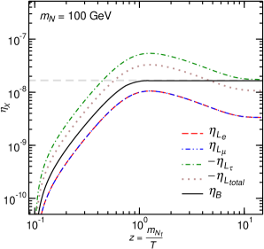
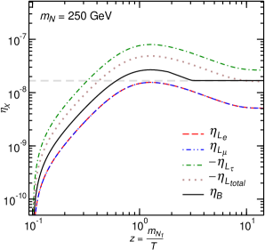
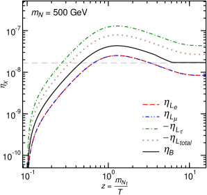
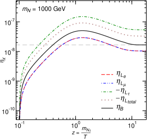
Figure 2: The predicted evolution of $\eta_{L_{l}}$ and $\eta_{B}$, for models with $m_{N}=$ 100, 250, 500 and 1000 GeV, and $\eta_{N_{\alpha}}^{\mathrm{in}}=1$. The model parameters are given in (5.1), (5.2), and Tables 2 and 3. The horizontal grey dashed line shows the baryon asymmetry needed to agree with observational data.

The BEs are solved numerically, using the Fortran code LeptoGen. Fig. 2 shows the predicted evolution of the baryon and individual lepton asymmetries, $\eta_{B}$ and $\eta_{L_{l}}$, as functions of the $T$-related parameter $z=m_{N_{1}}/T$, for each of the 4 examples, with $m_{N}=$ 100, 250, 500 and 1000 GeV. The specific model parameters are given in (5.1), (5.2), and Tables 2 and 3. Each scenario had an initially thermal heavy Majorana neutrino abundance and zero initial baryon and lepton asymmetries, i.e. $\eta_{N_{\alpha}}^{\mathrm{in}}=1$ and $\eta_{B}^{\mathrm{in}}=\eta_{L_{l}}^{\mathrm{in}}=0$. The 4 panels show that the large $L_{\tau}$ asymmetry is slightly reduced by less significant, but opposite sign $L_{e}$ and $L_{\mu}$ asymmetries. Clearly visible in each scenario is the effect of the rapidly decreasing rate of $B+L$ violation; the lepton and baryon asymmetries quickly decouple at $T\sim T_{c}$. This decoupling is particularly pronounced in the $m_{N}=100$ GeV scenario where the baryon asymmetry freezes out exactly when the lepton asymmetry is maximal. In particular, the rapid decoupling of $\eta_{B}$ from $\eta_{L_{l}}$ at temperatures $T$ close to $T_{c}$ has the virtue that, unlike $\eta_{L_{l}}$, $\eta_{B}$ remains almost unaffected from ordinary SM mass effects due to a non-zero VEV $v(T)$ [cf. (4.2)], since it is $v(T\sim T_{c})\ll v(T=0)$.

Figure 3: The (in)dependence of the final baryon asymmetry on the initial lepton, baryon and heavy Majorana neutrino abundances for (a) $m_{N}=$ 250 GeV and (b) $m_{N}=$ 100 GeV. The model parameters and the meaning of the horizontal grey line are the same as in Fig. 2.

Fig. 3 shows the evolution of the baryon asymmetry for varying initial lepton, baryon and heavy neutrino abundances. For the 250 GeV scenario, Fig. 3(a) illustrates the near independence of the resultant baryon asymmetry on the initial conditions. Even for the most extreme initial conditions $\eta^{\mathrm{in}}_{L_{l}}=\mp\,0.1$ and $\eta^{\mathrm{in}}_{B}=\pm\,0.1$, the variation in the final baryon asymmetry is only $\pm\,38\%$.

For heavy neutrino masses $m_{N}\stackrel{{\scriptstyle<}}{{{}_{\sim}}}250$ GeV, the dependence on initial conditions becomes stronger. In the $m_{N}=100$ GeV scenario, Fig. 3(b) shows the dependence of the final BAU on the initial lepton and baryon asymmetries in a R$\tau$L scenario with $m_{N}=100$ GeV. It is interesting to observe that the final $B$ asymmetry will remain almost unaffected, even if the primordial baryon asymmetry $\eta^{\mathrm{in}}_{B}$ at $T\stackrel{{\scriptstyle>}}{{{}_{\sim}}}10\,m_{N}$ is as large as $10^{-6}$, namely two orders of magnitude larger than the one required to agree with observational data.

In R$\tau$L scenarios with $m_{N}>250$ GeV, the final baryon asymmetry is completely independent of the initial conditions. This is illustrated in Fig. 4 for the R$\tau$L scenario with $m_{N}=$ 500 GeV. In this numerical example, it is most striking to notice that the prediction for the final BAU remains unchanged, even if the initial conditions are set at temperatures below the heavy neutrino mass scale $m_{N}$, e.g. at $T\sim 0.5\,m_{N}$.

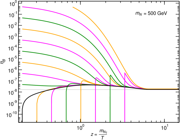
Figure 4: The complete independence of the final BAU on the initial lepton and baryon abundances for the $m_{N}=500$ GeV scenario, with model parameters the same as in Fig. 2.

Some insight into the independence on initial conditions is provided by Fig. 5. The ratios of various collision terms to the Hubble parameter are plotted for the $m_{N}=$ 250 GeV scenario. These ratios show that RL can take place almost completely in thermal equilibrium; in certain cases, the reaction rates are many orders of magnitude above the Hubble parameter $H(z=1)$. In spite of this fact, RL (R$\tau$L) can successfully generate the required excess in $L$ ($L_{\tau}$), because of the resonantly enhanced CP asymmetry.

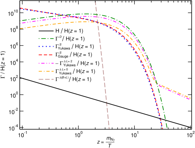
Figure 5: The ratio of various collision terms to the Hubble parameter plotted for the $m_{N}=250$ GeV scenario presented in Fig. 2.

To allow for a simple quantitative understanding of the baryon asymmetry in R$\tau$L (and similar) scenarios, we need to introduce the individual lepton flavour $K$-factors

$$K^{l}_{N_{\alpha}}\ =\ \frac{\Gamma(N_{\alpha}\to L_{l}\Phi)\>+\>\Gamma(N_{\alpha}\to L^{C}_{l}\Phi^{\dagger})}{H(z=1)}\ .$$ (5.6)

Note that the decay widths are calculated in terms of the one-loop resummed effective Yukawa couplings [17].

$K_{N_{\alpha}}^{l}$			$\alpha$
		1	2	3
	$e$	$1.0\times 10^{10}$	$1.0\times 10^{10}$	$25$
$l$	$\mu$	$1.4\times 10^{9}$	$1.4\times 10^{9}$	$20$
	$\tau$	$2.5$	$2.5$	$5.0$

Table 4: Individual lepton flavour $K$-factors for the $m_{N}=250$ GeV scenario.

Table 4 shows the various components of $K_{N_{\alpha}}^{l}$ for the $m_{N}=$ 250 GeV scenario. This explicitly demonstrates how the texture provided by (2.5) and (2.7) allows for a heavy Majorana neutrino to decay relatively out of equilibrium, whilst simultaneously protecting the $\tau$-lepton number from being washed-out, even though large $e$- and $\mu$-Yukawa couplings to $N_{1,2}$ exist. Bear in mind that we use the convention $m_{N_{1}}<m_{N_{2}}<m_{N_{3}}$ upon diagonalization of the heavy Majorana neutrino mass matrix $M_{S}$. As can be seen from Table 4, $K$-factors $K^{e,\mu,\tau}_{N_{3}}\sim 10$–100 and a CP-asymmetry $\delta_{N_{3}}^{\tau}\sim-10^{-6}$ are sufficient to generate a large $\tau$-lepton asymmetry. Although the $K$-factors $K^{e,\mu}_{N_{1,2}}$ associated with $N_{1,2}$ and the $e$ and $\mu$ leptons are enormous of order $10^{9}$–$10^{10}$, these turn out to be harmless to the $\tau$-lepton asymmetry, as the latter is protected by the low $\tau$-lepton $K$-factors $K^{\tau}_{N_{1,2,3}}\sim 10$.

An order of magnitude estimate of the final baryon asymmetry, including single lepton flavour effects, may be obtained using

$$\eta_{B}\ \sim\ -\,10^{-2}\,\times\,\sum_{l=1}^{3}\,\sum_{N_{\alpha}}\>e^{-(m_{N_{\alpha}}-m_{N_{1}})/m_{N_{1}}}\,\delta^{l}_{N_{\alpha}}\>\frac{K^{l}_{N_{\alpha}}}{K_{l}\,K_{N_{\alpha}}}\ .$$ (5.7)

The above estimate for $\eta_{B}$ is also consistent with the one stated earlier in [26]. In (5.7), the $K$-factors are summed in the following way:

$$K_{N_{\alpha}}\! = \!\sum_{l=1}^{3}\ K^{l}_{N_{\alpha}}\;,\qquad K_{l}\ =\ \sum_{N_{\alpha}}\,e^{-(m_{N_{\alpha}}-m_{N_{1}})/m_{N_{1}}}\,K^{l}_{N_{\alpha}}\;.$$ (5.8)

Notice that all $K$-factors are evaluated at $T=m_{N_{1}}$ (i.e. $z=m_{N_{1}}/T=1$), where $m_{N_{1}}$ is the lightest of the heavy Majorana neutrinos. The intuitive estimate (5.7) is applicable for all leptogenesis scenarios satisfying the approximate inequality

$$K_{lN_{\alpha}}\ \stackrel{{\scriptstyle>}}{{{}_{\sim}}}\ 1\,,$$ (5.9)

for each of the lepton flavours $l$ and the heavy Majorana neutrinos $N_{1,2,3}$. The inequality (5.9) ensures that the energy scale $m_{N_{1}}$ can be identified as the true scale of leptogenesis.

In RL scenarios, such as R$\tau$L, the importance of taking individual lepton flavour effects into account can be demonstrated by comparing (5.7) with the naive estimate, in which lepton flavour effects are treated indiscriminately in a universal manner,

$$\eta^{\,\mathrm{univ.}}_{B}\ \sim\ -\,10^{-2}\,\times\,\sum_{N_{\alpha}}\>e^{-(m_{N_{\alpha}}-m_{N_{1}})/m_{N_{1}}}\,\frac{\delta_{N_{\alpha}}}{K}\,,$$ (5.10)

where $K=\sum_{l=e,\mu\,\tau}K_{l}$. In the R$\tau$L scenario with $m_{N}=250$ GeV, the dominant contribution to this estimate will come from $N_{3}$, with a total CP asymmetry $\delta_{N_{3}}\sim 10^{-3}$. Taking the ratio of the two estimates yields

$$\frac{\eta^{\,\mathrm{univ.}}_{B}}{\eta_{B}}\ \sim\ \frac{\delta_{N_{3}}}{\delta^{\tau}_{N_{3}}}\,\frac{K_{N_{3}}\,K_{\tau}}{K^{\tau}_{N_{3}}\,K}\ \approx\ \frac{\delta_{N_{3}}}{\delta^{\tau}_{N_{3}}}\,\frac{|c|^{2}}{|a|^{2}+|b|^{2}}\ \approx\ -\,10^{-6}\,.$$ (5.11)

Thus, without considering single lepton flavour effects in this particular R$\tau$L model, one obtains an erroneous prediction for the BAU, which is suppressed by 6 orders of magnitude and has the wrong sign. These estimates are confirmed by solving the total lepton number BEs presented in [17].

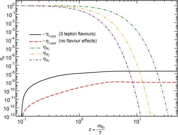
Figure 6: The predicted evolution of $\eta_{L_{\rm total}}$ and $\eta_{N_{\alpha}}$ for a model with a heavy neutrino spectrum: $m_{N_{3}}=3\,m_{N_{1}}$, $m_{N_{2}}=2\,m_{N_{1}}$ and $m_{N_{1}}=10^{10}$ GeV.

In a hierarchical scenario, the number densities of the heavier neutrinos $N_{2,3}$ at $T=m_{N_{1}}$ will be Boltzmann suppressed. To account for this phenomenon, we have included the Boltzmann factors $e^{-(m_{N_{\alpha}}-m_{N_{1}})/m_{N_{1}}}$ in the estimates (5.7), (5.10) and in the definition of $K_{l}$. Clearly, in RL models with each heavy neutrino nearly degenerate in mass, this last factor can be set to 1.

Flavour effects can also play a significant role in mildly hierarchical scenarios. Figure 6 shows the predicted evolution of the lepton asymmetry in a scenario where $m_{N_{3}}=3\,m_{N_{1}}$, $m_{N_{2}}=2\,m_{N_{1}}$ and $m_{N_{1}}=10^{10}$ GeV. The Yukawa texture was chosen to be consistent with light neutrino data and a normal hierarchical light neutrino spectrum. In this example, neglecting individual lepton flavour effects introduces an ${\cal O}(10)$ suppression of the final lepton and baryon asymmetry.

In fully hierarchical scenarios satisfying (5.9), it can be seen that the estimates (5.7) and (5.10) are completely equivalent. A large hierarchy in the heavy neutrino spectrum, combined with the condition (5.9), implies that the final lepton asymmetry is determined entirely by the decay of the lightest heavy Majorana neutrino $N_{1}$. This fact makes it impossible for a single lepton flavour to be protected from wash-out, whilst the neutrino decays out of equilibrium.

Likewise, in flavour universal scenarios, where $\eta_{L_{e,\mu,\tau}}=\frac{1}{3}\eta_{L}$, the estimates (5.7) and (5.10) are completely equivalent for both nearly degenerate and hierarchical leptogenesis scenarios.

Our numerical analysis presented in this section has explicitly demonstrated that models of R$\tau$L can provide a viable explanation for the observed BAU, in accordance with the current light neutrino data. In the next section, we will see how the scenarios considered here have far reaching phenomenological implications for low-energy observables of lepton flavour/number violation and collider experiments.

6 Phenomenological Implications

RL models, and especially R$\tau$L models, can give rise to a number of phenomenologically testable signatures. In particular, we will analyze the generic predictions of R$\tau$L models for the $0\nu\beta\beta$ decay, and for the LFV processes: $\mu\to e\gamma$, $\mu\to eee$ and $\mu\to e$ conversion in nuclei. Finally, we will present simple and realistic numerical estimates of production cross sections of heavy Majorana neutrinos at future $e^{+}e^{-}$ and $\mu^{+}\mu^{-}$ colliders, and apply these results to the R$\tau$L models.

6.1 $0\nu\beta\beta$ Decay

Neutrinoless double beta decay ($0\nu\beta\beta$) corresponds to a process in which two single $\beta$ decays [56, 57, 58] occur simultaneously in one nucleus. As a consequence of this, a nucleus $(Z,A)$ gets converted into a nucleus $(Z+2,A)$, i.e.

$${}^{A}_{Z}\,X\ \to\ ^{A}_{Z+2}\,X\>+\>2e^{-}\;.$$

Evidently, this process violates $L$-number by two units and can naturally take place in minimal RL models, in which the observed light neutrinos are Majorana particles. The observation of such a process would provide further information on the structure of the light neutrino mass matrix ${\bf m}^{\nu}$.

To a very good approximation, the half life for a $0\nu\beta\beta$ decay mediated by light Majorana neutrinos is given by

$$[T^{0\nu\beta\beta}_{1/2}]^{-1}\ =\ \frac{|\langle m\rangle|^{2}}{m^{2}_{e}}\ |{\cal M}_{0\nu\beta\beta}|^{2}\,G_{01}\;,$$ (6.1)

where $\langle m\rangle$ denotes the effective Majorana neutrino mass, $m_{e}$ is the electron mass and ${\cal M}_{0\nu\beta\beta}$ and $G_{01}$ denote the appropriate nuclear matrix element and the phase space factor, respectively. More details regarding the calculation of $T^{0\nu\beta\beta}_{1/2}$ may be found in [56, 57, 58].

In models of interest to us, the effective neutrino mass can be related to the entry $\{11\}\ (\equiv\{ee\})$ of the light neutrino mass matrix ${\bf m}^{\nu}$ in (2.8), i.e.

$$|\langle m\rangle|\ =\ |({\bf m}^{\nu})_{ee}|\ =\ \frac{v^{2}}{2m_{N}}\>\bigg{|}\,\frac{\Delta m_{N}}{m_{N}}\,a^{2}\ -\ \varepsilon^{2}_{e}\,\bigg{|}\;.$$ (6.2)

As has been explicitly demonstrated in the previous section, R$\tau$L models realize a light neutrino mass spectrum with an inverted hierarchy [59], thus giving rise to a sizeable effective neutrino mass. The prediction for $|\langle m\rangle|$ in these models is

$$|\langle m\rangle|\ =\ |({\bf m}^{\nu})_{ee}|\ \approx\ 0.013~{}{\rm eV}\;.$$ (6.3)

Such a prediction lies at the very low end of the value of the effective Majorana neutrino mass, reported recently by the Heidelberg–Moscow collaboration [60]. There are proposals for future $0\nu\beta\beta$-decay experiments that will be sensitive to values of $|\langle m\rangle|$ of order $10^{-2}$ [36], significantly increasing the constraints on this parameter.

6.2 $\mu\to e\gamma$

As shown in Fig. 7, heavy Majorana neutrinos may induce LFV couplings to the photon ($\gamma$) and the $Z$ boson via loop effects. These couplings give rise to LFV decays, such as $\mu\to e\gamma$ [61] and $\mu\to eee$ [62]. Our discussion and notation closely follows the extensive studies [62, 63]. Related phenomenological analyses of LFV effects in the SM with singlet neutrinos may be found in [64, 65, 66, 67].

Figure 7: Feynman graphs pertaining to the effective $\gamma e\mu$ and $Ze\mu$ couplings.

To properly describe LFV in low-energy observables, we first introduce the so-called Langacker–London (LL) parameters [68]:

$$(s^{\nu_{l}}_{L})^{2}\ =\ 1\,-\,\sum_{l^{\prime}=e,\mu,\tau}\,|B_{l\nu_{l^{\prime}}}|^{2}\ \approx\ \Big{(}m^{*}_{D}\,M^{*\,-1}_{S}\,M^{-1}_{S}\,m^{T}_{D}\Big{)}_{ll}\ ,$$ (6.4)

where $m_{D}=\frac{1}{\sqrt{2}}\,h^{\nu_{R}}\,v$ and $B_{l\nu_{l}^{\prime}}$ are mixing-matrix factors close to 1 that multiply the SM tree-level $Wl\nu_{l^{\prime}}$ vertices [39]. The LL parameters $(s^{\nu_{l}}_{L})^{2}$ quantify the deviation of the actual squared $Wl\nu_{l^{\prime}}$ couplings (summed over all light neutrinos) from the corresponding sum of squared couplings in the SM. The parameters $(s^{\nu_{e,\mu,\tau}}_{L})^{2}$ are constrained by LEP and low-energy electroweak observables [68, 69]. Independent constraints on these parameters typically give: $(s^{\nu_{e,\mu,\tau}}_{L})^{2}\stackrel{{\scriptstyle<}}{{{}_{\sim}}}10^{-2}$. As we will see in a moment, however, LFV observables impose much more severe constraints on products of the LL parameters, and especially on $s^{\nu_{e}}_{L}\,s^{\nu_{\mu}}_{L}$.

As a first LFV observable, we consider the decay $\mu\to e\gamma$. The branching fraction for the decay $\mu\to e\gamma$ is given by

$$B(\mu\to e\gamma)\ =\ \frac{\alpha^{3}_{w}s^{2}_{w}}{256\pi^{2}}\,\frac{m^{4}_{\mu}}{M^{4}_{W}}\,\frac{m_{\mu}}{\Gamma_{\mu}}\,|G_{\gamma}^{\mu e}|^{2}\ \approx\ \frac{\alpha^{3}_{w}s^{2}_{w}}{1024\pi^{2}}\,\frac{m^{4}_{\mu}}{M^{4}_{W}}\,\frac{m_{\mu}}{\Gamma_{\mu}}\;(s_{L}^{\nu_{\mu}})^{2}(s_{L}^{\nu_{e}})^{2}\,,$$ (6.5)

where $\Gamma_{\mu}=2.997\times 10^{-19}$ GeV [11] is the experimentally measured muon decay width, and $G_{\gamma}^{\mu e}$ is a composite form-factor defined in [62]. In arriving at the last equality in (6.5), we have assumed that $m^{2}_{N}\gg M^{2}_{W}$, for a model with two nearly degenerate heavy Majorana neutrinos. In this case, one finds that $G_{\gamma}^{\mu e}\to\frac{e^{i\phi}}{2}\,s_{L}^{\nu_{\mu}}s_{L}^{\nu_{e}}$, where $\phi$ is an unobservable model-dependent phase. Confronting the theoretical prediction (6.5) with the experimental upper limit [11]

$$B_{\rm exp}(\mu\to e\gamma)\ <\ 1.2\,\times 10^{-11}\,,\quad$$ (6.6)

we obtain the following constraint:

$$s_{L}^{\nu_{e}}s_{L}^{\nu_{\mu}}\ <\ 1.2\times 10^{-4}\,.$$ (6.7)

This last constraint is stronger by one to two orders of magnitude with respect to those derived on $(s_{L}^{\nu_{e}})^{2}$ and $(s_{L}^{\nu_{\mu}})^{2}$ individually.

In R$\tau$L models, only two of the right-handed neutrinos, $\nu_{2R}$ and $\nu_{3R}$, which have appreciable $e$- and $\mu$-Yukawa couplings, will be relevant to LFV effects. In this case, the LL parameters $(s_{L}^{\nu_{e}})^{2}$ and $(s_{L}^{\nu_{\mu}})^{2}$ are, to a very good approximation, given by

$$(s_{L}^{\nu_{e}})^{2}\ =\ \frac{|a|^{2}\,v^{2}}{m^{2}_{N}}\;,\qquad(s_{L}^{\nu_{\mu}})^{2}\ =\ \frac{|b|^{2}\,v^{2}}{m^{2}_{N}}\;.$$ (6.8)

Then, the following theoretical prediction is obtained:

$$B(\mu\to e\gamma)\ =\ 9\cdot 10^{-4}\,\times\,\frac{|a|^{2}\,|b|^{2}\,v^{4}}{m^{4}_{N}}\ .$$ (6.9)

For the particular scenarios considered in Section 5, we find $B(\mu\to e\gamma)\sim 10^{-12}$. These values are well within reach of the MEG collaboration, which will be sensitive to $B(\mu\to e\gamma)\sim 10^{-14}$ [34].

6.3 $\mu\to eee$

As illustrated in Fig. 8, quantum effects mediated by heavy Majorana neutrinos may also give rise to the 3-body LFV decay mode $\mu^{-}\to e^{-}e^{+}e^{-}$. The branching ratio for this LFV decay may conveniently be expressed as

$$B(\mu\to eee) = \frac{\alpha_{w}^{4}}{24576\pi^{3}}\ \frac{m_{\mu}^{4}}{M_{W}^{4}}\ \frac{m_{\mu}}{\Gamma_{\mu}}\bigg{\{}\,2|{\textstyle\frac{1}{2}}F_{\rm box}^{\mu eee}+F_{Z}^{\mu e}-2s_{w}^{2}(F_{Z}^{\mu e}-F_{\gamma}^{\mu e})|^{2}$$ (6.10)

$$+\,4s_{w}^{4}|F_{Z}^{\mu e}-F_{\gamma}^{\mu e}|^{2}\,+\,16s_{w}^{2}\>{\rm Re}\Big{[}(F_{Z}^{\mu e}+{\textstyle\frac{1}{2}}F_{\rm box}^{\mu eee})G_{\gamma}^{\mu e\>\ast}\Big{]}$$

$$-\,48s_{w}^{4}\>{\rm Re}\Big{[}\,(F_{Z}^{\mu e}-F_{\gamma}^{\mu e})G_{\gamma}^{\mu e\>\ast}\,\Big{]}\,+\,32s_{w}^{4}|G_{\gamma}^{\mu e}|^{2}\>\bigg{(}\ln\frac{m_{\mu}^{2}}{m_{e}^{2}}-\frac{11}{4}\bigg{)}\,\bigg{\}}\;.\qquad$$

The expressions $F_{\gamma}^{\mu e}$, $F_{Z}^{\mu e}$ and $F_{\rm box}^{\mu eee}$ are composite form-factors, defined and computed in [62]. In the limit $m^{2}_{N}\gg M^{2}_{W}$ and up to an overall physically irrelevant phase factor $e^{i\phi}$, these composite form-factors simplify to [62]

$$F_{\gamma}^{\mu e} \approx -\,\frac{7}{12}\,s_{L}^{\nu_{\mu}}s_{L}^{\nu_{e}}\,-\,\frac{1}{6}\,s_{L}^{\nu_{\mu}}s_{L}^{\nu_{e}}\ln\bigg{(}\frac{m^{2}_{N}}{M^{2}_{W}}\bigg{)}\,,$$ (6.11)

$$F_{Z}^{\mu e} \approx \bigg{[}\,\frac{5}{2}\,-\,\frac{3}{2}\,\ln\bigg{(}\frac{m^{2}_{N}}{M^{2}_{W}}\bigg{)}\,\bigg{]}\,s_{L}^{\nu_{\mu}}s_{L}^{\nu_{e}}\ -\ \frac{1}{2}s_{L}^{\nu_{\mu}}s_{L}^{\nu_{e}}\sum_{k=e,\mu,\tau}\ (s_{L}^{\nu_{k}})^{2}\>\frac{m^{2}_{N}}{M^{2}_{W}}\,,$$ (6.12)

$$F_{\rm box}^{\mu eee} \approx -2\,s_{L}^{\nu_{\mu}}s_{L}^{\nu_{e}}\ +\ \frac{1}{2}\;s_{L}^{\nu_{\mu}}s_{L}^{\nu_{e}}(s_{L}^{\nu_{e}})^{2}\>\frac{m^{2}_{N}}{M^{2}_{W}}\;.$$ (6.13)

Correspondingly, the analytic result (6.10) in the same limit may be cast into the form:

$$B(\mu\to eee)\! \simeq \!\frac{\alpha_{w}^{4}}{294912\,\pi^{3}}\ \frac{m_{\mu}^{4}}{M_{W}^{4}}\ \frac{m_{\mu}}{\Gamma_{\mu}}\ (s_{L}^{\nu_{\mu}})^{2}(s_{L}^{\nu_{e}})^{2}\>\Bigg{\{}\,54-300s_{w}^{2}+217s_{w}^{4}+96\,s_{w}^{4}\ln\bigg{(}\frac{m_{\mu}^{2}}{m_{e}^{2}}\bigg{)}$$ (6.14)

$$-\>\Big{(}108-492s_{w}^{2}+800s_{w}^{4}\Big{)}\ln\bigg{(}\frac{m^{2}_{N}}{M^{2}_{W}}\bigg{)}+\ \Big{(}54-192s_{w}^{2}+256s_{w}^{4}\Big{)}\ln^{2}\bigg{(}\frac{m^{2}_{N}}{M^{2}_{W}}\bigg{)}$$

$$+\ \frac{m^{2}_{N}}{M^{2}_{W}}\ \Bigg{[}\,\bigg{(}18-50s_{w}^{2}-\Big{(}18-32s_{w}^{2}\Big{)}\ln\bigg{(}\frac{m^{2}_{N}}{M^{2}_{W}}\bigg{)}\bigg{)}\ (s_{L}^{\nu_{e}})^{2}$$

$$-\>\bigg{(}36-172s_{w}^{2}+300s_{w}^{4}-\Big{(}36-136s_{w}^{2}+192s_{w}^{4}\Big{)}\ln\bigg{(}\frac{m^{2}_{N}}{M^{2}_{W}}\bigg{)}\bigg{)}\sum_{l=e,\mu,\tau}(s_{L}^{\nu_{l}})^{2}\Bigg{]}$$

$$+\>\frac{m^{4}_{N}}{M^{4}_{W}}\ \Bigg{[}\,\frac{3}{2}(s_{L}^{\nu_{e}})^{4}\ -\ 6\,(1-2s^{2}_{w})(s_{L}^{\nu_{e}})^{2}\sum_{l=e,\mu,\tau}(s_{L}^{\nu_{l}})^{2}$$

$$+\>6\,\Big{(}1-4s_{w}^{2}+6s^{4}_{w}\Big{)}\Big{(}\sum_{l=e,\mu,\tau}(s_{L}^{\nu_{l}})^{2}\Big{)}^{2}\,\Bigg{]}\,\Bigg{\}}\;.$$

It can be seen from (6.14) that the so-called non-decoupling terms proportional to $m^{4}_{N}/M^{4}_{W}$ are always multiplied with higher powers of the LL parameters. In general, these terms do not decouple and become very significant [62], for large heavy neutrino masses $m_{N}$ and fixed values of $s^{\nu_{l}}_{L}$, which amounts to scenarios with large neutrino Yukawa couplings $|h^{\nu_{R}}_{ij}|\stackrel{{\scriptstyle>}}{{{}_{\sim}}}0.5$ [39]. However, these non-decoupling terms are negligible, as long as $s^{\nu_{l}}_{L}\,m_{N}/M_{W}\ll 1$. This is actually the case for the R$\tau$L models discussed in Section 5. Neglecting terms proportional to $m^{2}_{N}/M^{2}_{W}$ and $m^{4}_{N}/M^{4}_{W}$, we may relate $B(\mu\to eee)$ to $B(\mu\to e\gamma)$ through:

$$B(\mu\to eee)\ \simeq\ 8.2\cdot 10^{-3}\,\times\Bigg{[}\,1\ -\ 0.8\ln\bigg{(}\frac{m^{2}_{N}}{M^{2}_{W}}\bigg{)}\ +\ 0.5\ln^{2}\bigg{(}\frac{m^{2}_{N}}{M^{2}_{W}}\bigg{)}\,\Bigg{]}\>B(\mu\to e\gamma)\;.$$ (6.15)

For example, for an R$\tau$L model with $m_{N}=250$ GeV, (6.15) implies

$$B(\mu\to eee)\ \simeq\ 1.4\cdot 10^{-2}\,\times B(\mu\to e\gamma)\ \simeq\ 1.4\cdot 10^{-14}$$ (6.16)

This value is a factor $\sim 70$ below the present experimental bound [11]: $B_{\rm exp}(\mu\to eee)<1.0\times 10^{-12}$. In this respect, it would be very encouraging, if higher sensitivity experiments could be designed to probe this observable.

Figure 8: Feynman graphs responsible for $\mu^{-}\to e^{-}e^{+}e^{-}$ ($\mu\to e$ conversion in nuclei).

6.4 Coherent $\mu\to e$ Conversion in Nuclei

One of the most sensitive experiments to LFV is the coherent conversion of $\mu\to e$ in nuclei, e.g. $\mu^{-}\ {}^{48}_{22}{\rm Ti}\to e^{-}\ {}^{48}_{22}{\rm Ti}$ [70, 71]. The Feynman graphs responsible for such a process are displayed in Fig. 8.

Our calculation of $\mu\to e$ conversion in nuclei closely follows [70, 71, 63]. We consider the kinematic approximations: $q^{2}\approx-m^{2}_{\mu}$ and $p^{0}_{e}\approx|\vec{p}_{e}|\approx m_{\mu}$, which are valid for $\mu\to e$ conversion. Given the above approximation, the $\mu\to e$ conversion rate in a nucleus with nucleon numbers $(N,Z)$, is given by

$$B_{\mu e}(N,Z)\ \equiv\ \frac{\Gamma[\mu\,(N,Z)\to e\,(N,Z)]}{\Gamma[\mu\,(N,Z)\to{\rm capture}]}\ \approx\ \frac{\alpha^{3}_{\rm em}\alpha^{4}_{w}m^{5}_{\mu}}{32\pi^{2}M^{4}_{W}\Gamma_{\rm capt.}}\,\frac{Z^{4}_{\rm eff}}{Z}\,|F(-m^{2}_{\mu})|^{2}\,|Q_{W}|^{2}\,,$$ (6.17)

where $\alpha_{\rm em}=1/137$ is the electromagnetic fine structure constant, $Z_{\rm eff}$ is the effective atomic number of coherence and $\Gamma_{\rm capt.}$ is the muon nuclear capture rate. For ${}^{48}_{22}{\rm Ti}$, experimental measurements give $Z_{\rm eff}\approx 17.6$ for ${}^{48}_{22}{\rm Ti}$ [72] and $\Gamma[\mu\ {}^{48}_{22}{\rm Ti}\to{\rm capture}]\approx 1.705\times 10^{-18}$ GeV [73]. Moreover, $|F(-m^{2}_{\mu})|\approx 0.54$ is the nuclear form factor [74]. Finally, $Q_{W}=V_{u}(2Z+N)+V_{d}(Z+2N)$ is the coherent charge of the nucleus, which is associated with the vector current. Its explicit form is given by

$$V_{u} = \frac{2}{3}\,s^{2}_{w}\,\Big{(}\,F^{\mu e}_{\gamma}\,-\,G^{\mu e}_{\gamma}\,-\,F^{\mu e}_{Z}\,\Big{)}\,+\,\frac{1}{4}\,\Big{(}\,F^{\mu e}_{Z}\,-\,F^{\mu euu}_{\rm box}\,\Big{)}\,,$$ (6.18)

$$V_{d} = -\,\frac{1}{3}\,s^{2}_{w}\,\Big{(}\,F^{\mu e}_{\gamma}\,-\,G^{\mu e}_{\gamma}\,-\,F^{\mu e}_{Z}\,\Big{)}\,-\,\frac{1}{4}\,\Big{(}\,F^{\mu e}_{Z}\,+\,F^{\mu edd}_{\rm box}\,\Big{)}\,.$$ (6.19)

The composite form-factors $F^{\mu euu}_{\rm box}$ and $F^{\mu edd}_{\rm box}$ are defined in [63]. In the SM with two nearly degenerate heavy Majorana neutrinos and in the limit $m^{2}_{N}/M^{2}_{W}\gg 1$, these form-factors can be written down in the simplified forms:

$$F_{\rm box}^{\mu euu}\ \approx\ F_{\rm box}^{\mu edd}\ \approx\ -\,s_{L}^{\nu_{\mu}}s_{L}^{\nu_{e}}\;.$$ (6.20)

In the same limit $m^{2}_{N}/M^{2}_{W}\gg 1$, $B_{\mu e}(N,Z)$ is given by

$$B_{\mu e}(N,Z) \simeq \frac{\alpha^{3}_{\rm em}\alpha^{4}_{w}m^{5}_{\mu}}{18432\,\pi^{2}M^{4}_{W}\Gamma_{\rm capt.}}\,\frac{Z^{4}_{\rm eff}}{Z}\,|F(-m^{2}_{\mu})|^{2}\,(s_{L}^{\nu_{\mu}})^{2}(s_{L}^{\nu_{e}})^{2}$$ (6.21)

$$\times\,\Bigg{\{}\,\bigg{[}\,3N+(33-86s_{w}^{2})Z+\Big{(}9N-(9-32s_{w}^{2})Z\Big{)}\ln\bigg{(}\frac{m^{2}_{N}}{M^{2}_{W}}\bigg{)}\bigg{]}^{2}$$

$$+\ 6\ \frac{m^{2}_{N}}{M^{2}_{W}}\bigg{[}\,3N+(33-86s_{w}^{2})Z+\Big{(}9N-(9-32s_{w}^{2})Z\Big{)}\ln\bigg{(}\frac{m^{2}_{N}}{M^{2}_{W}}\bigg{)}\bigg{]}$$

$$\times\ \Big{(}N-(1-4s_{w}^{2})Z\Big{)}\ \sum_{l=e,\mu,\tau}(s_{L}^{\nu_{l}})^{2}$$

$$+\ 9\ \frac{m^{4}_{N}}{M^{4}_{W}}\ \Big{(}N-(1-4s_{w}^{2})Z\Big{)}^{2}\ \Big{(}\sum_{l=e,\mu,\tau}(s_{L}^{\nu_{l}})^{2}\Big{)}^{2}\,\Bigg{\}}\;.$$

For the ${}^{48}_{22}{\rm Ti}$ case, $B_{\mu e}(26,22)$ is related to $B(\mu\to e\gamma)$ through

$$B_{\mu e}(26,22)\ \simeq\ 0.1\,\times\Bigg{[}\,1\ +\ 0.5\ \ln\bigg{(}\frac{m^{2}_{N}}{M^{2}_{W}}\bigg{)}\Bigg{]}^{2}\>B(\mu\to e\gamma)\;.$$ (6.22)

On the experimental side, the strongest upper bound on $B_{\mu e}(N,Z)$ is obtained from experimental data on $\mu\to e$ conversion in ${}^{48}_{22}{\rm Ti}$ [75]:

$$B^{\rm exp}_{\mu e}(26,22)\ <\ 4.3\,\times 10^{-12}\,,$$ (6.23)

at the 90% CL. However, the proposed experiment by the MECO collaboration [35] will be sensitive to conversion rates of order $10^{-16}$.

In the R$\tau$L model with $m_{N}=250$ GeV, one obtains, on the basis of (6.22), the prediction for $\mu\to e$ conversion in ${}^{48}_{22}{\rm Ti}$:

$$B_{\mu e}(26,22)\ \simeq\ 0.46\times B(\mu\to e\gamma)\ \sim\ 4.5\times 10^{-13}\;.$$ (6.24)

The above prediction falls well within reach of the sensitivity proposed by the MECO collaboration.

$m_{N}$ (GeV)	$B(\mu\to e\gamma)$	$B(\mu\to eee)$	$B_{\mu e}(26,22)$
$100$	$6.2\times 10^{-12}$	$3.8\times 10^{-14}$	$9.2\times 10^{-13}$
$250$	$9.9\times 10^{-13}$	$1.4\times 10^{-14}$	$4.5\times 10^{-13}$
$500$	$2.5\times 10^{-13}$	$9.7\times 10^{-15}$	$2.0\times 10^{-13}$
$1000$	$6.2\times 10^{-14}$	$4.9\times 10^{-15}$	$7.7\times 10^{-14}$

Table 5: Branching fractions for the 3 LFV processes $\mu\to e\gamma$, $\mu\to eee$ and coherent $\mu\to e$ conversion in ${}^{48}_{22}{\rm Ti}$ nuclei.

In Table 5, we summarize our results for the branching ratios of the 3 LFV processes: $\mu\to e\gamma$, $\mu\to eee$ and coherent $\mu\to e$ conversion in ${}^{48}_{22}{\rm Ti}$ nuclei, for each R$\tau$L model considered in Section 5.

As a final general remark, we should mention that R$\tau$L models, and leptogenesis models in general, do not suffer from too large contributions to the electron electric dipole moment (EDM) [12, 76], which first arises at two loops. The reason is that EDM effects are suppressed either by higher powers of small Yukawa couplings of order $10^{-4}$ and less, or by very small factors, such as $(m_{N_{1}}-m_{N_{2,3}})/m_{N}\sim 10^{-7}$. The latter is the case in R$\tau$L models, which leads to unobservably small EDM effects of order $10^{-37}~{}e$ cm, namely 10 orders of magnitude smaller than the present experimental limits [11].

6.5 Collider Heavy Majorana Neutrino Production

If heavy Majorana neutrinos have electroweak-scale masses and appreciable couplings to electrons and muons they can be copiously produced at future $e^{+}e^{-}$ [77, 78] and $\mu^{+}\mu^{-}$ colliders. As shown in Fig. 9, this is exactly the kinematic situation for the heavy Majorana neutrinos $N_{2,3}$ described by the R$\tau$L models. The heavy Majorana neutrino $N_{1}$ has a very small coupling to leptons and it would be very difficult to produce this state directly.

Figure 9: Diagrams related to the production of the heavy Majorana neutrinos $N_{2,3}$ at future $e^{+}e^{-}(\mu^{+}\mu^{-})$ high-energy colliders.

For collider c.m.s. energies $\sqrt{s}\gg m_{N}$, the $t$-channel $W^{-}$-boson exchange graphs will dominate over the $Z$-boson exchange graph, which is $s$-channel propagator suppressed (see Fig. 9). In this high-energy limit, the production cross section for heavy Majorana neutrinos approaches a constant [77], i.e.

$$\sigma\Big{[}\,e^{+}e^{-}\,(\mu^{+}\mu^{-})\to N_{2,3}\,\nu\,\Big{]}\ \approx\ \frac{\pi\,\alpha^{2}_{w}}{4\,M^{2}_{W}}\>(s^{\nu_{e(\mu)}}_{L})^{2}\ \approx\ 10~{}{\rm fb}\,\times\,\Bigg{(}\,\frac{s^{\nu_{e(\mu)}}_{L}}{10^{-2}}\,\Bigg{)}^{2}\ .$$ (6.25)

Since $s^{\nu_{\tau}}_{L}\approx 0$ in R$\tau$L models, the produced heavy Majorana neutrinos $N_{2,3}$ will have the characteristic signature that they will predominantly decay into electrons and muons, but not into $\tau$ leptons. Assuming that $m_{N}\stackrel{{\scriptstyle>}}{{{}_{\sim}}}M_{H}$, the branching fraction of $N_{2,3}$ decays into charged leptons and into $W^{\pm}$ bosons decaying hadronically is

$$B\Big{(}N_{2,3}\to e^{\mp},\,\mu^{\mp}\,W^{\pm}(\to{\rm jets})\Big{)}\ \approx\ \frac{1}{2}\,\times\,\frac{2}{3}\ =\ \frac{1}{3}\;.$$ (6.26)

Given (6.25), (6.26) and an integrated luminosity of 100 fb^-1, we expect to be able to analyze about 100 signal events for $(s^{\nu_{e(\mu)}}_{L})^{2}=10^{-2}$ and $m_{N}\stackrel{{\scriptstyle<}}{{{}_{\sim}}}300$ GeV, at future $e^{+}e^{-}$ and $\mu^{+}\mu^{-}$ colliders with c.m.s. energy $\sqrt{s}=0.5$–$1~{}{\rm TeV}$.

These simple estimates are supported by a recent analysis, where competitive background reactions to the signal have been considered [78]. This analysis showed that the inclusion of background processes reduces the number of signal events by a factor of 10. The authors in [78] find that an $e^{+}e^{-}$ linear collider with c.m.s. energy $\sqrt{s}=0.5$ TeV will be sensitive to values of $s^{\nu_{e}}_{L}=|a|v/m_{N}\sim 0.7\times 10^{-2}$. This amounts to the same level of sensitivity to the parameter $|a|$, for R$\tau$L scenarios with $m_{N}=250$ GeV. The sensitivity to $s^{\nu_{e}}_{L}$ could be improved by a factor of 3, i.e. $s^{\nu_{e}}_{L}\sim 0.2\times 10^{-2}$, in proposed upgraded $e^{+}e^{-}$ accelerators such as CLIC.

A similar analysis should be envisaged to hold for future $\mu^{+}\mu^{-}$ colliders, leading to similar findings for $s^{\nu_{\mu}}_{L}=|b|v/m_{N}$. In general, we expect that the ratio of the two production cross sections of $N_{2,3}$ at the two colliders under identical conditions of c.m.s. energy and luminosity will give a direct measure of the ratio of $|a|^{2}/|b|^{2}$. This information, together with that obtained from low-energy LFV observables, $0\nu\beta\beta$-decay experiments, and neutrino data, will significantly constrain the parameters of the R$\tau$L models. Finally, since the heavy Majorana neutrinos $N_{2,3}$ play an important synergetic role in resonantly enhancing $\delta^{\tau}_{N_{1}}$, potentially large CP asymmetries in their decays will determine the theoretical parameters of these models further. Evidently, more detailed studies are needed before one could reach a definite conclusion concerning the exciting possibility that electroweak-scale R$\tau$L models may naturally constitute a laboratory testable solution to the cosmological problem of the BAU.

7 Conclusions

We have studied a novel variant of RL, which may take place at the electroweak phase transition. This RL variant gives rise to a number of phenomenologically testable signatures for low-energy experiments and future high-energy colliders. The new RL scenario under study makes use of the property that, in addition to $B-L$ number, sphalerons preserve the individual quantum numbers $\frac{1}{3}B-L_{e,\mu,\tau}$ [28]. The observed BAU can be produced by lepton-to-baryon conversion of an individual lepton number. For the case of the $\tau$-lepton number this mechanism has been called resonant $\tau$-leptogenesis [26].

In studying leptogenesis, we have extended previous analyses of the relevant network of BEs. More explicitly, we have consistently taken into account SM chemical potential effects, as well as effects from out of equilibrium sphalerons and single lepton flavours. In particular, we have found that single lepton flavour effects become very important in R$\tau$L models. In this case, the difference between our improved formalism of BEs and the usual formalism followed in the literature could be dramatic. The predictions of the usual formalism could lead to an erroneous result which is suppressed by many orders of magnitude. The suppression factor could be enormous of order $10^{-6}$ for the R$\tau$L scenarios considered in Section 5. Even within leptogenesis models with a mild hierarchy between the heavy neutrino masses, the usual formalism turns out to be inadequate to properly treat single lepton flavour effects; its predictions may differ even up to one order of magnitude with respect to those obtained with our improved formalism.

One generic feature of R$\tau$L models is that their predictions for the final baryon asymmetry are almost independent of the initial values for the primordial $B$-number, $L$-number and heavy Majorana neutrino abundances. Specifically, we have investigated the dependence of the BAU on the initial conditions, as a function of the heavy neutrino mass scale $m_{N}$. We have found that for $m_{N}\stackrel{{\scriptstyle>}}{{{}_{\sim}}}250$ GeV, the dependence of the BAU is always less than 7%, even if the initial baryon asymmetry is as large as $\eta^{\rm in}_{B}=10^{-2}$ at $z=m_{N}/T=0.1$. For smaller values of $m_{N}$, this dependence starts getting larger. Thus, for $m_{N}=100$ GeV, the dependence of the final baryon asymmetry on the initial conditions is stronger, unless the primordial baryon asymmetry is smaller than $\sim 10^{-6}$ at $z=0.1$.

In order to have successful leptogenesis in the R$\tau$L models under study, the heavy Majorana neutrinos are required to be nearly degenerate. This nearly degenerate heavy neutrino mass spectrum may be obtained by enforcing an SO(3) symmetry, which is explicitly broken by the Yukawa interactions to a particular SO(2) sub-group isomorphic to a lepton-type group U(1)_l. The approximate breaking of U(1)_l, which could result from a FN mechanism, leads to a Yukawa texture that accounts for the existing neutrino oscillation data, except those from the LSND experiment [79]. Our choice of the breaking parameters was motivated by the naturalness of the light and heavy neutrino sectors. To obtain natural R$\tau$L models, we have followed the principle that there should be no excessive cancellations between tree-level and radiative or thermal effects. In this way, we have found that R$\tau$L models strongly favour a light neutrino mass spectrum with an inverted hierarchy. Moreover, when the same naturalness condition is applied to the heavy neutrino sector, a particular hierarchy for the mass differences of the heavy Majorana neutrinos is obtained. In particular, the mass difference of one pair of heavy Majorana neutrinos is much smaller than the other two possible pairs.

R$\tau$L models offer a number of testable phenomenological signatures for low-energy experiments and future high-energy colliders. These models contain electroweak-scale heavy Majorana neutrinos with appreciable couplings to electrons and muons, e.g. $N_{1,2}$. Specifically, the (normalized to the SM) $W^{\pm}$-boson couplings of electrons and muons to the heavy Majorana neutrinos $N_{1,2}$ could be as large as 0.01, for $m_{N_{1,2}}=100$–300 GeV. As a consequence, these heavy Majorana particles can be produced at future $e^{+}e^{-}$ and $\mu^{+}\mu^{-}$ colliders, operating with a c.m.s. energy $\sqrt{s}=0.5$–1 TeV. Another feature of R$\tau$L models is that thanks to the inverted hierarchic structure of the light neutrino mass spectrum, they can account for sizeable $0\nu\beta\beta$ decay. The predicted effective neutrino mass $|({\bf m}^{\nu})_{ee}|$ can be as large as 0.02 eV, which is within the sensitivity of the proposed next round of $0\nu\beta\beta$ decay experiments. The most striking phenomenological feature of 3-generation (non-supersymmetric) R$\tau$L models is that they can predict $e$- and $\mu$-number-violating processes, such as the decay $\mu\to e\gamma$ and $\mu\to e$ conversion in nuclei, with observable rates. In particular, these LFV effects could be as large as $10^{-12}$ for $B(\mu\to e\gamma)$ and as large as $5\times 10^{-13}$ for a $\mu\to e$ conversion rate in ${}^{48}_{22}$Ti, normalized to the $\mu$ capture rate. The above predicted values are within reach of the experiments proposed by the MEG and MECO collaborations.

Although the present study improves previous analyses of the BEs related to leptogenesis models, there are still some additional smaller but relevant effects that would require special treatment. The first obvious improvement would be to calculate the thermal effects on the collision terms, beyond the HTL approximation. These corrections would eliminate some of the uncertainties pertinent to the actual choice of the IR regulator in some of the collision terms. These effects limit the accuracy of our predictions and introduce an estimated theoretical uncertainty of 30% for leptogenesis models operating well above the electroweak phase transition, with relatively large $K$ factors, i.e. $K_{lN_{\alpha}}\stackrel{{\scriptstyle>}}{{{}_{\sim}}}5$. For models at the electroweak phase transition, the IR problem is less serious, but larger uncertainties may enter due to the lack of a satisfactorily accurate quantitative framework for sphaleron dynamics. Although the implementation of the sphaleron dynamics in our BEs for RL models was based on the calculations of [33, 27, 30], particular treatment would be needed, if the electroweak phase transition was a strong first-order one. In this case, the dynamics of the expanding bubbles during the electroweak phase transition becomes relevant [80]. This possibility may emerge in supersymmetric versions of RL models. Nevertheless, the inclusion of the aforementioned additional effects is expected not to modify the main results of the present analysis drastically and will be the subject of a future communication.

Acknowledgements

We thank Mikko Laine, Costas Panagiotakopoulos, Graham Ross, Kiriakos Tamvakis and Carlos Wagner for useful discussions and comments. The work of AP has been supported in part by the PPARC research grants: PPA/G/O/2002/00471 and PP/C504286/1. The work of TU has been funded by the PPARC studentship PPA/S/S/2002/03469.

Appendix A Collision Terms

A.1 Useful Notation and Definitions

The following notation and definitions are used in the derivation of the BEs. The number density, $n_{a}$, of a particle species, $a$, with $g_{a}$ internal degrees of freedom is given by [45]

$$n_{a}(T) = g_{a}\,\int\frac{d^{3}{\bf p}}{(2\pi)^{3}}\ \exp\Big{[}-\Big{(}\sqrt{{\bf p}^{2}+m^{2}_{a}}-\mu_{a}(T)\Big{)}/T\,\Big{]}$$ (A.1)

$$= \frac{g_{a}\,m^{2}_{a}\,T\ e^{\mu_{a}(T)/T}}{2\pi^{2}}\ K_{2}\bigg{(}\frac{m_{a}}{T}\bigg{)}\;,$$

where $\mu_{a}$ is the $T$-dependent chemical potential and $K_{n}(x)$ is the $n$th-order modified Bessel function [81]. In our minimal leptogenesis model, the factors $g_{a}$ are: $g_{W^{a}}=3g_{B}=6$ and $g_{\Phi}=g_{\Phi^{\dagger}}=2$, and for the $i$th family: $g_{N_{\alpha}}=2$, $g_{L_{i}}=g_{L^{C}_{i}}=4$, $g_{Q_{i}}=g_{Q^{C}_{i}}=12$, and $g_{u_{i}}=g_{u_{i}^{C}}=6$. Using the same formalism as [17] the CP-conserving collision term for a generic process $X\to Y$ and its CP-conjugate $\overline{X}\to\overline{Y}$ is defined as

$$\gamma^{X}_{Y}\ \equiv\ \gamma(X\to Y)\>+\>\gamma(\overline{X}\to\overline{Y})\;,$$ (A.2)

with

$$\gamma(X\to Y)\ =\ \int\!d\pi_{X}\,d\pi_{Y}\,(2\pi)^{4}\,\delta^{(4)}(p_{X}-p_{Y})\ e^{-p^{0}_{X}/T}\,|{\cal M}(X\to Y)|^{2}\;.$$ (A.3)

In the above, $|{\cal M}(X\to Y)|^{2}$ is the squared matrix element which is summed but not averaged over the internal degrees of freedom of the initial and final multiparticle states $X$ and $Y$. Moreover, $d\pi_{X}$ represents the phase space factor of a multiparticle state $X$,

$$d\pi_{X}\ =\ \frac{1}{S_{X}}\,\prod\limits_{i=1}^{n_{X}}\,\frac{d^{4}p_{i}}{(2\pi)^{3}}\ \delta(p^{2}_{i}-m^{2}_{i})\;\theta(p^{0}_{i})\;,$$ (A.4)

where $S_{X}=n_{\rm id}!$ is a symmetry factor depending on the number of identical particles, $n_{\rm id}$, contained in $X$.

As CPT is preserved, the CP-conserving collision term $\gamma^{X}_{Y}$ obeys the relation

$$\gamma^{X}_{Y}\ =\ \gamma^{Y}_{X}\,.$$ (A.5)

Analogously, it is possible to define a CP-violating collision term $\delta\gamma^{X}_{Y}$ as

$$\delta\gamma^{X}_{Y}\ \equiv\ \gamma(X\to Y)\ -\ \gamma(\overline{X}\to\overline{Y})\ =\ -\,\delta\gamma^{Y}_{X}\;,$$ (A.6)

where the last equality follows from CPT invariance.

A.2 CP-Conserving Collision Terms

In numerically solving the BEs, we introduce the dimensionless parameters:

$$z\ =\ \frac{m_{N_{1}}}{T}\,,\quad x\ =\ \frac{s}{m_{N_{1}}^{2}}\,,\quad a_{\alpha}\ =\ \left(\frac{m_{N_{\alpha}}}{m_{N_{1}}}\right)^{2},\quad a_{r}\ =\ \left(\frac{m_{\rm IR}}{m_{N_{1}}}\right)^{2},\quad c^{\,l}_{\alpha}\ =\ \left(\,\frac{\Gamma^{\,l}_{N_{\alpha}}}{m_{N_{1}}}\,\right)^{2},$$ (A.7)

where $\alpha=1,2,3$ labels the heavy Majorana neutrino states, $s$ is the usual Mandelstam variable and $m_{\rm IR}$ is an infra-red (IR) mass regulator which is discussed below.

In terms of the resummed effective Yukawa couplings $(\bar{h}^{\nu}_{\pm})_{l\alpha}$ introduced in [17], the radiatively corrected decay width $\Gamma_{N_{\alpha}}^{\,l}$ of a heavy Majorana neutrino $N_{\alpha}$ into a lepton flavour $l$ is given by

$$\Gamma_{N_{\alpha}}^{\,l}\ =\ \frac{m_{N_{\alpha}}}{16\pi}\ \Big{[}\,(\bar{h}^{\nu}_{+})^{*}_{l\alpha}\,(\bar{h}^{\nu}_{+})_{l\alpha}\>+\>(\bar{h}^{\nu}_{-})^{*}_{l\alpha}\,(\bar{h}^{\nu}_{-})_{l\alpha}\,\Big{]}\;.$$ (A.8)

By means of (A.3), the $1\to 2$ CP-conserving collision term $\gamma^{N_{\alpha}}_{L_{l}\Phi}$ is found to be

$$\gamma^{N_{\alpha}}_{L_{l}\Phi}\ =\ \gamma(N_{\alpha}\to L_{l}\Phi)\>+\>\gamma(N_{\alpha}\to L^{C}_{l}\Phi^{\dagger})\! = \!\Gamma^{\,l}_{N_{\alpha}}\,g_{N_{\alpha}}\,\int\frac{d^{3}{\bf p}_{N_{\alpha}}}{(2\pi)^{3}}\,\frac{m_{N_{\alpha}}}{E_{N_{\alpha}}({\bf p})}\,e^{-E_{N_{\alpha}}({\bf p})/T}$$ (A.9)

$$= \!\frac{m^{4}_{N_{1}}a_{i}\,\sqrt{c^{\,l}_{i}}}{\pi^{2}\,z}\ K_{1}(z\sqrt{a_{i}})\,,$$

where $E_{N_{\alpha}}({\bf p})=\sqrt{{\bf p}^{2}+m^{2}_{N_{\alpha}}}$ and $g_{N_{\alpha}}=2$ is the number of internal degrees of freedom of $N_{\alpha}$. Upon summation over lepton flavours $l$, this collision term reduces to the corresponding one given in (B.4) of [17].

For $2\to 2$ processes, one can make use of the reduced cross section $\widehat{\sigma}(s)$ defined as

$$\widehat{\sigma}(s)\ \equiv\ 8\pi\,\Phi(s)\int\!d\pi_{Y}\>(2\pi)^{4}\,\delta^{(4)}(q-p_{Y})\>\left|{\cal M}(X\rightarrow Y)\right|^{2}\;,$$ (A.10)

where $s=q^{2}$ and the initial phase space integral is given by

$$\Phi(s)\ \equiv\ \int\!d\pi_{X}\>(2\pi)^{4}\,\delta^{(4)}(p_{X}-q)\,.$$ (A.11)

These expressions simplify to give

$$\widehat{\sigma}(s)\ =\ \frac{1}{8\pi s}\ \int\limits_{t_{-}}^{t_{+}}\!dt\ \left|{\cal M}(X\rightarrow Y)\right|^{2}\;,$$ (A.12)

where $t$ is the usual Mandelstam variable, and the phase-space integration limits $t_{\pm}$ will be specified below.

In processes, such as $N_{\alpha}V_{\mu}\to L_{l}\Phi$, the exchanged particles (e.g. $L$ and $\Phi$) occurring in the $t$ and $u$ channels are massless. These collision terms possess IR divergences at the phase-space integration limits $t_{\pm}$ in (A.12). Within a more appropriate framework, such as finite temperature field theory, these IR singularities would have been regulated by the thermal masses of the exchanged particles. In our $T=0$ field theory calculation, we have regulated the IR divergences by cutting off the phase-space integration limits $t_{\pm}$ using a universal thermal regulator $m_{\rm IR}$ related to the expected thermal masses of the exchanged particles. This procedure preserves chirality and gauge invariance, as would be expected within the framework of a finite temperature field theory [43].

Thermal masses for the Higgs and leptons are predominantly generated by gauge and top-quark Yukawa interactions. In the HTL approximation, they are given by [44]

$$\frac{m^{2}_{L}(T)}{T^{2}} = \frac{1}{32}\,\Big{(}3\,g^{2}+g^{\prime\,2}\Big{)}\,,$$

$$\frac{m_{\Phi}^{2}(T)}{T^{2}} = 2d\,\Bigg{(}1-\frac{T_{c}^{2}}{T^{2}}\Bigg{)}\,,$$ (A.13)

where $d=(8M_{W}^{2}+M_{Z}^{2}+2m_{t}^{2}+M_{H}^{2})/(8v^{2})$. In our numerical estimates, we choose the regulator $m_{\rm IR}$ to vary between the lepton and Higgs thermal masses, evaluated at $T\approx m_{N}$. The resulting variation in the predicted baryon asymmetry can be taken as a contribution to the theoretical uncertainties in our zero temperature calculation.

For reduced cross-sections with an apparent singularity at the upper limit $t_{+}$, the following upper and lower limits are used:

$$t_{+}\ =\ -m_{\rm IR}^{2}\,,\qquad t_{-}\ =\ m_{N_{\alpha}}^{2}-s\,.$$ (A.14)

Likewise, for reduced cross-sections with apparent singularities at both the upper and lower limits $t_{\pm}$, the following limits are employed:

$$t_{+}\ =\ -m_{\rm IR}^{2}\,,\qquad t_{-}\ =\ m_{N_{\alpha}}^{2}+m_{\rm IR}^{2}-s\;.$$ (A.15)

It is important to remark here that the collision terms do not suffer from IR singularities at $T\stackrel{{\scriptstyle<}}{{{}_{\sim}}}T_{c}$, because the leptons, $W$ and $Z$ bosons receive $v(T)$-dependent masses during the electroweak phase transition. The full implementation of such effects will be given elsewhere.

Substituting (A.10) and (A.11) into (A.3), one obtains

$$\gamma^{X}_{Y}\ =\ \frac{m^{4}_{N_{1}}}{64\,\pi^{4}z}\ \int\limits_{x_{\rm thr}}^{\infty}\!dx\ \sqrt{x}\;K_{1}(z\sqrt{x})\;\widehat{\sigma}^{X}_{Y}(x)\;,$$ (A.16)

where $x_{\rm thr}$ is the kinematic threshold for a given $2\to 2$ process.

For $2\to 2$ $\Delta L=1$ processes, one can repeat the procedure in [17] (Appendix B), without summing over lepton flavours. Each $\Delta L=1$ process has an identical factor dependent on $\bar{h}^{\nu}_{\pm}$. To produce the $\Delta L=1$ collision terms for each lepton flavour, this factor needs to be replaced with its un-summed equivalent,

$$(\bar{h}^{\nu}_{+})^{*}_{l\alpha}\,(\bar{h}^{\nu}_{+})_{l\alpha}\>+\>(\bar{h}^{\nu}_{-})^{*}_{l\alpha}\,(\bar{h}^{\nu}_{-})_{l\alpha}\,,$$ (A.17)

exactly as was done in (A.8). The remainder of the analytic expression for each of these terms is presented in [17].

In addition to the Higgs and gauge mediated $\Delta L=1$ terms, there are also $2\to 2$ $\Delta L=2$ processes. As before, these processes are $L_{k}\Phi\leftrightarrow L_{l}^{C}\Phi^{\dagger}$ and $L_{k}L_{l}\leftrightarrow\Phi^{\dagger}\Phi^{\dagger}$ where the former has its real intermediate states subtracted. The analytic forms of these collision terms are identical to the total lepton number case but lepton flavour is not summed over. The reduced cross sections are given by

$$\widehat{\sigma}^{\,\prime\,L_{k}\Phi}_{L_{l}^{C}\Phi^{\dagger}}\!\! = \!\!\sum_{\alpha,\beta=1}^{3}\ {\rm Re}\,\Bigg{\{}\,\bigg{[}\,(\bar{h}^{\nu}_{+})^{*}_{k\alpha}\,(\bar{h}^{\nu}_{+})_{k\beta}\,(\bar{h}^{\nu}_{+})^{*}_{l\alpha}\,(\bar{h}^{\nu}_{+})_{l\beta}\>+\>(\bar{h}^{\nu}_{-})^{*}_{k\alpha}\,(\bar{h}^{\nu}_{-})_{k\beta}\,(\bar{h}^{\nu}_{-})^{*}_{l\alpha}\,(\bar{h}^{\nu}_{-})_{l\beta}\,\bigg{]}\>\mathcal{A}^{(ss)}_{\alpha\beta}$$ (A.18)

$$\qquad\qquad+\>2\,\bigg{[}\,(\bar{h}^{\nu}_{+})^{*}_{l\alpha}\,h^{\nu}_{l\beta}\,(\bar{h}^{\nu}_{+})^{*}_{k\alpha}\,h^{\nu}_{k\beta}\>+\>(\bar{h}^{\nu}_{-})^{*}_{l\alpha}\,h^{\nu*}_{l\beta}\,(\bar{h}^{\nu}_{-})^{*}_{k\alpha}\,h^{\nu*}_{k\beta}\,\bigg{]}\mathcal{A}^{(st)*}_{\alpha\beta}$$

$$\qquad\qquad+\>2\,\Big{(}h^{\nu*}_{k\alpha}\,h^{\nu}_{k\beta}\,h^{\nu*}_{l\alpha}\,h^{\nu}_{l\beta}\Big{)}\;\mathcal{A}^{(tt)}_{\alpha\beta}\,\Bigg{\}}\,,$$

and

$$\widehat{\sigma}^{L_{k}L_{l}}_{\Phi^{\dagger}\Phi^{\dagger}}\ =\ \sum_{\alpha,\beta=1}^{3}\;{\rm Re}\,\Big{(}h^{\nu*}_{k\alpha}\,h^{\nu}_{k\beta}\,h^{\nu*}_{l\alpha}\,h^{\nu}_{l\beta}\Big{)}\;\mathcal{B}_{\alpha\beta}\;,$$ (A.19)

where the $\mathcal{A}$ and $\mathcal{B}$ factors are presented in [17].

As we now consider lepton flavours separately, it is necessary to include $\Delta L=0$, but lepton flavour violating interactions. The three lowest order $2\leftrightarrow 2$ processes are shown diagrammatically in Figure 10: $L_{k}\Phi\leftrightarrow L_{l}\Phi$, $L_{k}\Phi^{\dagger}\leftrightarrow L_{l}\Phi^{\dagger}$ and $L_{k}L^{C}_{l}\leftrightarrow\Phi^{\dagger}\Phi$ (note that $k\neq l$). The first of these reactions contains heavy Majorana neutrinos as RISs. These need be removed using the procedure outlined in [17]. The reduced cross section for each of these processes is

$$\widehat{\sigma}^{\,\prime\,L_{k}\Phi}_{\,L_{l}\Phi}=\sum_{\alpha,\beta=1}^{3}\Big{[}(\bar{h}^{\nu}_{+})^{*}_{l\alpha}\,(\bar{h}^{\nu}_{-})^{*}_{k\alpha}\,(\bar{h}^{\nu}_{+})_{l\beta}\,(\bar{h}^{\nu}_{-})_{k\beta}+(\bar{h}^{\nu}_{-})^{*}_{l\alpha}\,(\bar{h}^{\nu}_{+})^{*}_{k\alpha}\,(\bar{h}^{\nu}_{-})_{l\beta}\,(\bar{h}^{\nu}_{+})_{k\beta}\Big{]}\,\mathcal{C}_{\alpha\beta}$$ (A.20)

with

$$\mathcal{C}_{\alpha\beta}\ =\ \left\{\begin{array}[]{lc}\frac{\displaystyle xa_{\alpha}}{\displaystyle 4\pi|D^{2}_{\alpha}|}\ \to\ 0&\quad(\alpha=\beta)\\[14.22636pt] \frac{\displaystyle x\sqrt{a_{\alpha}\,a_{\beta}}}{\displaystyle 4\pi P^{*}_{\alpha}P_{\beta}}&\quad(\alpha\neq\beta)\end{array}\right.$$ (A.21)

In (A.21), $P^{-1}_{\alpha}(x)$ is the Breit–Wigner $s$-channel propagator

$$P_{\alpha}^{-1}(x)\ =\ \frac{1}{x-a_{\alpha}+i\sqrt{a_{\alpha}c_{\alpha}}}\ .$$ (A.22)

Therefore, following the procedure in [17], the RIS-subtracted propagator is determined by

$$|D_{\alpha}^{-1}(x)|^{2}\ =\ |P_{\alpha}^{-1}(x)|^{2}-\frac{\pi}{\sqrt{a_{\alpha}c_{\alpha}}}\,\delta(x-a_{\alpha})\ \to\ 0.$$ (A.23)

Figure 10: $\Delta L=0$ interactions between leptons of different flavours mediated by heavy Majorana neutrinos. (a) corresponds to the process $L_{k}\Phi\leftrightarrow L_{l}\Phi$, (b) corresponds to the process $L_{k}\Phi^{\dagger}\leftrightarrow L_{l}\Phi^{\dagger}$ and (c) corresponds to the process $L_{k}L^{C}_{l}\leftrightarrow\Phi^{\dagger}\Phi$.

Processes (b) and (c) in Fig. 10 do not contain RISs and have the following reduced cross sections:

$$\widehat{\sigma}^{\,L_{k}\Phi^{\dagger}}_{L_{l}\Phi^{\dagger}}\! = \!\sum_{\alpha,\beta=1}^{3}\mathrm{Re}\Big{(}h^{\nu*}_{l\alpha}\,h^{\nu}_{k\alpha}\,h^{\nu}_{l\beta}\,h^{\nu*}_{k\beta}\Big{)}\,\mathcal{D}_{\alpha\beta}\,,$$ (A.24)

$$\widehat{\sigma}^{\,L_{k}L^{C}_{l}}_{\Phi^{\dagger}\Phi}\! = \!\sum_{\alpha,\beta=1}^{3}\mathrm{Re}\Big{(}h^{\nu*}_{l\alpha}\,h^{\nu}_{k\alpha}\,h^{\nu}_{l\beta}\,h^{\nu*}_{k\beta}\Big{)}\,\mathcal{E}_{\alpha\beta}\,,$$ (A.25)

where for $\alpha\neq\beta$,

$$\mathcal{D}_{\alpha\beta}\! = \!\frac{\sqrt{a_{\alpha}a_{\beta}}}{\pi x(a_{\alpha}-a_{\beta})}\>\Bigg{[}\,(x+a_{\beta})\ln\Bigg{(}\frac{x+a_{\beta}}{a_{\beta}}\Bigg{)}-(x+a_{\alpha})\ln\Bigg{(}\frac{x+a_{\alpha}}{a_{\alpha}}\Bigg{)}\,\Bigg{]}\,,$$ (A.26)

$$\mathcal{E}_{\alpha\beta}\! = \!\frac{\sqrt{a_{\alpha}a_{\beta}}}{\pi(a_{\alpha}-a_{\beta})}\>\ln\Bigg{(}\frac{a_{\alpha}(x+a_{\beta})}{a_{\beta}(x+a_{\alpha})}\Bigg{)}\,,$$ (A.27)

and for $\alpha=\beta$,

$$\mathcal{D}_{\alpha\alpha}\! = \!\frac{a_{\alpha}}{\pi x}\>\Bigg{[}\,\frac{x}{a_{\alpha}}-\ln\Bigg{(}\frac{x+a_{\alpha}}{a_{\alpha}}\Bigg{)}\,\Bigg{]}\,,$$ (A.28)

$$\mathcal{E}_{\alpha\alpha}\! = \!\frac{x}{\pi(x+a_{\alpha})}\,.$$ (A.29)

References

- [1] D.N. Spergel et al., Astrophys. J. Suppl. 148 (2003) 175.
-
[2]
For recent reviews, see,
W. Buchmüller, R. D. Peccei and T. Yanagida, hep-ph/0502169;
M. Dine and A. Kusenko, Rev. Mod. Phys. 76 (2004) 1;
K. Enqvist and A. Mazumdar, Phys. Rept. 380 (2003) 99. - [3] M. Fukugita and T. Yanagida, Phys. Lett. B 174 (1986) 45.
-
[4]
P. Minkowski, Phys. Lett. B 67 (1977) 421;
M. Gell-Mann, P. Ramond and R. Slansky, in Supergravity, eds. D.Z. Freedman and P. van Nieuwenhuizen (North-Holland, Amsterdam, 1979);
T. Yanagida, in Proc. of the Workshop on the Unified Theory and the Baryon Number in the Universe, Tsukuba, Japan, 1979, eds. O. Sawada and A. Sugamoto;
R. N. Mohapatra and G. Senjanović, Phys. Rev. Lett. 44 (1980) 912. - [5] V. A. Kuzmin, V. A. Rubakov and M. E. Shaposhnikov, Phys. Lett. B 155 (1985) 36.
-
[6]
For an alternative suggestion, see,
R. Allahverdi, S. Hannestad, A. Jokinen, A. Mazumdar and S. Pascoli,
hep-ph/0504102. - [7] S. Davidson and A. Ibarra, Phys. Lett. B 535 (2002) 25.
- [8] W. Buchmüller, P. Di Bari and M. Plümacher, Nucl. Phys. B 643 (2002) 367.
- [9] G.C. Branco, R. Gonzalez Felipe, F.R. Joaquim, I. Masina, M.N. Rebelo and C.A. Savoy, Phys. Rev. D 67 (2003) 073025.
-
[10]
P.H. Chankowski and K. Turzynski, Phys. Lett. B
570 (2003) 198;
T. Hambye, Y. Lin, A. Notari, M. Papucci and A. Strumia, Nucl. Phys. B 695 (2004) 169. - [11] Particle Data Group (S. Eidelman et al.), Phys. Lett. B 592 (2004) 1.
- [12] A. Pilaftsis, Phys. Rev. D 56 (1997) 5431; Nucl. Phys. B 504 (1997) 61.
- [13] A. Pilaftsis, Int. J. Mod. Phys. A 14 (1999) 1811.
-
[14]
T. Hambye, Nucl. Phys. B 633 (2002) 171;
L. Boubekeur, hep-ph/0208003;
L. Boubekeur, T. Hambye and G. Senjanovic, Phys. Rev. Lett. 93 (2004) 111601;
A. Abada, H. Aissaoui and M. Losada, hep-ph/0409343;
L. J. Hall, H. Murayama and G. Perez, hep-ph/0504248. - [15] J. Liu and G. Segré, Phys. Rev. D 48 (1993) 4609.
-
[16]
M. Flanz, E.A. Paschos and U. Sarkar, Phys. Lett. B 345 (1995) 248;
L. Covi, E. Roulet and F. Vissani, Phys. Lett. B 384 (1996) 169. - [17] A. Pilaftsis and T.E.J. Underwood, Nucl. Phys. B 692 (2004) 303.
-
[18]
R.N. Mohapatra and J.W.F. Valle, Phys. Rev. D 34
(1986) 1642;
S. Nandi and U. Sarkar, Phys. Rev. Lett. 56 (1986) 564. - [19] C.D. Froggatt and H.B. Nielsen, Nucl. Phys. B 147 (1979) 277.
-
[20]
T. Hambye, J. March-Russell and S. M. West, JHEP 0407 (2004) 070;
S. M. West, Phys. Rev. D 71 (2005) 013004. -
[21]
J. R. Ellis, M. Raidal and T. Yanagida, Phys. Lett. B 546 (2002) 228;
Y. Grossman, T. Kashti, Y. Nir and E. Roulet, Phys. Rev. Lett. 91 (2003) 251801;
G. D’Ambrosio, G. F. Giudice and M. Raidal, Phys. Lett. B 575 (2003) 75;
E. J. Chun, Phys. Rev. D 69 (2004) 117303;
R. Allahverdi and M. Drees, Phys. Rev. D 69 (2004) 103522;
Y. Grossman, R. Kitano and H. Murayama, hep-ph/0504160. -
[22]
T. Dent, G. Lazarides and R. Ruiz de Austri, Phys. Rev. D 69 (2004) 075012;
S. Dar, S. Huber, V.N. Senoguz and Q. Shafi, Phys. Rev. D 69 (2004) 077701;
T. Dent, G. Lazarides and R. R. de Austri, hep-ph/0503235. - [23] R. Gonzalez Felipe, F. R. Joaquim and B. M. Nobre, Phys. Rev. D 70 (2004) 085009.
- [24] E. K. Akhmedov, M. Frigerio and A. Y. Smirnov, JHEP 0309 (2003) 021.
- [25] C.H. Albright and S.M. Barr, Phys. Rev. D 69 (2004) 073010.
- [26] A. Pilaftsis, Phys. Rev. Lett. 95 (2005) 081602.
- [27] S. Y. Khlebnikov and M. E. Shaposhnikov, Nucl. Phys. B 308 (1988) 885.
- [28] J.A. Harvey and M.S. Turner, Phys. Rev. D 42 (1990) 3344.
- [29] H. Dreiner and G.G. Ross, Nucl. Phys. B 410 (1993) 188.
- [30] M. Laine and M. E. Shaposhnikov, Phys. Rev. D 61 (2000) 117302.
-
[31]
For alternative suggestions, albeit in extended
supersymmetric settings, see,
F. Borzumati and Y. Nomura, Phys. Rev. D 64 (2001) 053005;
N. Arkani-Hamed, L. J. Hall, H. Murayama, D. R. Smith and N. Weiner, Phys. Rev. D 64 (2001) 115011. - [32] Under rather generic conditions, the reheating temperature in supersymmetric theories could be very low, even as low as TeV, because of the presence of quasi-flat directions with large VEV’s, which slow down the thermalization process in the early Universe [R. Allahverdi and A. Mazumdar, arXiv:hep-ph/0505050]. In such a scenario, electroweak-scale RL may be the only viable mechanism for successful baryogenesis.
- [33] L. Carson, X. Li, L. D. McLerran and R. T. Wang, Phys. Rev. D 42 (1990) 2127.
- [34] See proposal by MEG collaboration at http://meg.web.psi.ch/docs/index.html.
-
[35]
MECO collaboration, http://meco.ps.uci.edu/;
M. Hebert (MECO Collaboration), Nucl. Phys. A 721 (2003) 461. -
[36]
C. Aalseth et al., hep-ph/0412300;
S. Pascoli, S.T. Petcov and T. Schwetz, hep-ph/0505226. - [37] We thank Graham Ross for useful discussions on this point.
- [38] G. C. Branco, W. Grimus and L. Lavoura, Nucl. Phys. B 312 (1989) 492.
- [39] A. Pilaftsis, Z. Phys. C 55 (1992) 275.
- [40] A. Pilaftsis, Phys. Rev. D 65 (2002) 115013.
- [41] G. Pasarino and M. Veltman, Nucl. Phys. B 160 (1979) 151.
-
[42]
P. H. Chankowski and Z. Pluciennik,
Phys. Lett. B 316 (1993) 312;
K. S. Babu, C. N. Leung and J. T. Pantaleone, Phys. Lett. B 319 (1993) 191;
For recent studies, see,
S. Antusch, M. Drees, J. Kersten, M. Lindner and M. Ratz, Phys. Lett. B 519 (2001) 238;
S. Antusch, J. Kersten, M. Lindner, M. Ratz and M. A. Schmidt, JHEP 0503 (2005) 024. -
[43]
M. Le Bellac, Thermal Field Theory, (Cambridge
University Press, Cambridge, England, 1996);
J.I. Kapusta, Finite-Temperature Field Theory, (Cambridge University Press, Cambridge, England, 1989). - [44] H.A. Weldon, Phys. Rev. D 26 (1982) 2789.
- [45] E. W. Kolb and S. Wolfram, Nucl. Phys. B 172 (1980) 224 [Erratum-ibid. B 195 (1982) 542].
- [46] M. A. Luty, Phys. Rev. D 45 (1992) 455.
-
[47]
J. S. Schwinger,
J. Math. Phys. 2 (1961) 407;
L. V. Keldysh, Zh. Eksp. Teor. Fiz. 47 (1964) 1515 [Sov. Phys. JETP 20 (1965) 1018];
G. Raffelt, G. Sigl and L. Stodolsky, Phys. Rev. Lett. 70 (1993) 2363;
G. Sigl and G. Raffelt, Nucl. Phys. B 406 (1993) 423. - [48] W. Buchmuller and M. Plumacher, Phys. Lett. B 511 (2001) 74.
- [49] G. ’t Hooft, Phys. Rev. Lett. 37 (1976) 8.
- [50] P. Arnold and L. D. McLerran, Phys. Rev. D 36 (1987) 581.
- [51] J.M. Cline, K. Kainulainen and K.A. Olive, Phys. Rev. D 49 (1994) 6394.
- [52] F. R. Klinkhamer and N. S. Manton, Phys. Rev. D 30 (1984) 2212.
- [53] For a recent analysis, see, M. Maltoni, T. Schwetz, M. A. Tortola and J. W. Valle, New J. Phys. 6 (2004) 122.
- [54] R. Barbieri, P. Creminelli, A. Strumia and N. Tetradis, Nucl. Phys. B 575 (2000) 61.
- [55] G.F. Giudice, A. Notari, M. Raidal, A. Riotto and A. Strumia, Nucl. Phys. B 685 (2004) 89.
- [56] M. Doi, T. Kotani and E. Takasugi, Prog. Theor. Phys. Suppl. 83 (1985) 1.
- [57] For example, see the textbook by K. Grotz and H.V. Klapdor, “The Weak Interaction in Nuclear, Particle und Astrophysics,” (Adam Hilger, Bristol, 1989).
-
[58]
H.V. Klapdor-Kleingrothaus, “Sixty Years of Double Beta
Decay,” (World Scientific, Singapore, 2001);
H.V. Klapdor-Kleingrothaus, A. Dietz, H.L. Harney, I.V. Krivosheina, Mod. Phys. Lett. A 16 (2001) 2409;
H.V. Klapdor-Kleingrothaus, A. Dietz and I. Krivosheina, Particles and Nuclei 110 (2002) 57; Foundations of Physics 32 (2002) 1181. -
[59]
H.V. Klapdor-Kleingrothaus and U. Sarkar, Mod. Phys. Lett. A 16 (2001) 2469;
H.V. Klapdor-Kleingrothaus, H. Päs and A. Yu. Smirnov, Phys. Rev. D 63 (2001) 073005;
W. Rodejohann, Nucl. Phys. B 597 (2001) 110; J. Phys. G 28 (2002) 1477;
H. Minakata and H. Sugiyama, Phys. Lett. B 532 (2002) 275;
S. Pascoli and S.T. Petcov, Phys. Lett. B 544 (2002) 239;
H. Nunokawa, W. J. C. Teves and R. Zukanovich Funchal, Phys. Rev. D 66 (2002) 093010. - [60] H.V. Klapdor-Kleingrothaus, A. Dietz, I.V. Krivosheina and O. Chkvorets, Nucl. Instrum. Meth. A522 (2004) 371.
- [61] T.P. Cheng and L.F. Li, Phys. Rev. Lett. 45 (1980) 1908.
- [62] A. Ilakovac and A. Pilaftsis, Nucl. Phys. B 437 (1995) 491.
- [63] A. Ioannisian and A. Pilaftsis, Phys. Rev. D 62 (2000) 066001.
- [64] J.G. Körner, A. Pilaftsis and K. Schilcher, Phys. Lett. B 300 (1993) 381.
- [65] J. Bernabéu, J.G. Körner, A. Pilaftsis and K. Schilcher, Phys. Rev. Lett. 71 (1993) 2695.
-
[66]
A. Pilaftsis, Mod. Phys. Lett. A 9 (1994) 3595;
M.C. Gonzalez-Garcia and J.W.F. Valle, Mod. Phys. Lett. A 7 (1992) 477; Erratum 9 (1994) 2569. -
[67]
L.N. Chang, D. Ng and J.N. Ng, Phys. Rev. D 50 (1994) 4589;
G. Bhattacharya, P. Kalyniak and I. Mello, Phys. Rev. D 51 (1995) 3569;
A. Pilaftsis, Phys. Rev. D 52 (1995) 459;
A. Ilakovac, B.A. Kniehl, and A. Pilaftsis, Phys. Rev. D 52 (1995) 3993;
A. Ilakovac, Phys. Rev. D 54 (1996) 5653;
M. Frank and H. Hamidian, Phys. Rev. D 54 (1996) 6790;
P. Kalyniak and I. Mello, Phys. Rev. D 55 (1997) 1453;
G. Barenboim and M. Raidal, Nucl. Phys. B 484 (1997) 63;
Z. Gagyi-Palffy, A. Pilaftsis and K. Schilcher, Nucl. Phys. B 513 (1998) 517;
S. Fajfer and A. Ilakovac, Phys. Rev. D 57 (1998) 4219;
M. Raidal and A. Santamaria, Phys. Lett. B 421 (1998) 250;
M. Czakon, M. Zralek and J. Gluza, Nucl. Phys. B 573 (2000) 57;
J. I. Illana and T. Riemann, Phys. Rev. D 63 (2001) 053004;
G. Cvetic, C. Dib, C. S. Kim and J. D. Kim, Phys. Rev. D 66 (2002) 034008; hep-ph/0504126;
A. Masiero, S. K. Vempati and O. Vives, New J. Phys. 6 (2004) 202. - [68] P. Langacker and D. London, Phys. Rev. D 38 (1988) 886.
-
[69]
C. P. Burgess, S. Godfrey, H. Konig, D. London and I. Maksymyk, Phys. Rev. D 49 (1994) 6115;
E. Nardi, E. Roulet and D. Tommasini, Phys. Lett. B 327 (1994) 319;
D. Tommasini, G. Barenboim, J. Bernabeu and C. Jarlskog, Nucl. Phys. B 444 (1995) 451;
S. Bergmann and A. Kagan, Nucl. Phys. B 538 (1999) 368. -
[70]
G. Feinberg and S. Weinberg, Phys. Rev. Lett. 3
(1959) 111; 244 (Erratum);
W.J. Marciano and A.I. Sanda, Phys. Rev. Lett. 78 (1977) 1512;
O. Shanker, Phys. Rev. D 20 (1979) 1608;
J. Bernabéu, E. Nardi and D. Tommasini, Nucl. Phys. B 409 (1993) 69. -
[71]
For reviews, see, J.D. Vergados, Phys. Rep. 133
(1986) 1;
T.S. Kosmas, G.K. Leontaris and J.D. Vergados, Prog. Part. Nucl. Phys. 33 (1994) 397. -
[72]
J.C. Sens, Phys. Rev. 113 (1959) 679;
K.W. Ford and J.G. Wills, Nucl. Phys. 35 (1962) 295;
R. Pla and J. Bernabéu, An. Fís. 67 (1971) 455;
H.C. Chiang, E. Oset, T.S. Kosmas, A. Faessler and J.D. Vergados, Nucl. Phys. A 559 (1993) 526. - [73] T. Suzuki, D.F. Measday and J.P. Roalsvig, Phys. Rev. C 35 (1987) 2212.
- [74] For instance, see, B. Frois and C.N. Papanicolas, Ann. Rev. Nucl. Sci. 37 (1987) 133, and references therein.
- [75] C. Dohmen et al. (SINDRUM II Collaboration), Phys. Lett. B317 (1993) 631.
-
[76]
D. Ng and J.N. Ng, Mod. Phys. Lett. A 11 (1996) 211;
J.P. Archaumbault, A. Czarnecki and M. Pospelov, hep-ph/0406089;
W.-F. Chang and J.N. Ng, hep-ph/0411201. -
[77]
W. Buchmüller and C. Greub, Nucl. Phys. B 363
(1991) 345;
G. Cvetic, C.S. Kim and C.W. Kim, Phys. Rev. Lett. 82 (1999) 4761;
S. F. King and T. Yanagida, hep-ph/0411030. -
[78]
F. del Aguila, J. A. Aguilar-Saavedra, A. Martinez de la Ossa
and D. Meloni, Phys. Lett. B 613 (2005) 170;
F. del Aguila and J. A. Aguilar-Saavedra, hep-ph/0503026. - [79] A. Aguilar et al. (LSND Collaboration), Phys. Rev. D 64 (2001) 112007.
-
[80]
For recent analyses, see,
M. Carena, M. Quiros, M. Seco and C. E. M. Wagner, Nucl. Phys. B 650 (2003) 24;
T. Konstandin, T. Prokopec and M. G. Schmidt, Nucl. Phys. B 716 (2005) 373;
M. Carena, A. Megevand, M. Quiros and C. E. M. Wagner, Nucl. Phys. B 716 (2005) 319;
T. Konstandin, T. Prokopec, M. G. Schmidt and M. Seco, hep-ph/0505103. - [81] Handbook of Mathematical Functions, edited by M. Abramowitz and I. A. Stegun (Verlag Harri Deutsch, Frankfurt, 1984).