OUTP–0505P
TUM-HEP–591/05
hep–ph/0506102
Neutrinoless Double Beta Decay and Future Neutrino Oscillation Precision Experiments

Abstract

We discuss to what extent future precision measurements of neutrino mixing observables will influence the information we can draw from a measurement of (or an improved limit on) neutrinoless double beta decay. Whereas the $\Delta m^{2}$ corresponding to solar and atmospheric neutrino oscillations are expected to be known with good precision, the parameter $\theta_{12}$ will govern large part of the uncertainty. We focus in particular on the possibility of distinguishing the neutrino mass hierarchies and on setting a limit on the neutrino mass. We give the largest allowed values of the neutrino masses which allow to distinguish the normal from the inverted hierarchy. All aspects are discussed as a function of the uncertainty stemming from the involved nuclear matrix elements. The implications of a vanishing, or extremely small, effective mass are also investigated. By giving a large list of possible neutrino mass matrices and their predictions for the observables, we finally explore how a measurement of (or an improved limit on) neutrinoless double beta decay can help to identify the neutrino mass matrix if more precise values of the relevant parameters are known.

1 Introduction

The last few years have seen tremendous progress in our understanding of the neutrino sector. The solar neutrino deficit is now known to be certainly due to neutrino flavor oscillations [1, 2, 3, 4, 5, 6] with the best–fit oscillation parameters given as $\Delta m_{\odot}^{2}\equiv\Delta m^{2}_{21}=8.0\times 10^{-5}$ eV² and $\sin^{2}\theta_{\odot}\equiv\sin^{2}\theta_{12}=0.31$ [5]. The atmospheric neutrino deficit can also be ascribed to flavor oscillations with a good degree of confidence [7, 8] with the best–fit oscillation parameters as $\Delta m_{\rm atm}^{2}\equiv|\Delta m^{2}_{31}|=2.1\times 10^{-3}$ eV² and $\sin^{2}2\theta_{\rm atm}\equiv\sin^{2}2\theta_{23}=1$ [7]. The upper limit on the third mixing angle $\theta_{13}$ is mainly determined by the reactor neutrino data [9], which when combined with the information obtained from the solar and atmospheric neutrino experiments gives a bound of $\sin^{2}\theta_{13}<0.044$ at $3\sigma$ [10, 11].

Despite all these impressive achievements, there still remains a lot to be learned. The arguably most fundamental question, namely whether neutrinos are Dirac or Majorana particles, remains still to be answered. If neutrinos are Majorana particles, we have nine physical parameters describing the $3\times 3$ light neutrino mass matrix and determining them is one of the ultimate goals of neutrino physics. With the two $\Delta m^{2}$ and two mixing angles – $\theta_{12}$ and $\theta_{23}$ — known, there still remain five parameters to be tracked down. To be more precise, we still lack knowledge about the following points:

• Is there $CP$ violation in the lepton sector in analogy with that in the quark sector?

• Is the atmospheric neutrino mixing angle $\theta_{23}$ exactly maximal? If not, does it lie above or below $\pi/4$?

• Is the third mixing angle $\theta_{13}$ exactly zero?

• How small is the absolute neutrino mass scale?

• What is the ordering of the neutrino masses, i.e., what is the neutrino mass hierarchy?

Answers to all or some of these question will certainly lead to better understanding of the underlying theory which gives rise to neutrino masses.

Neutrinoless double beta decay (0$\nu\beta\beta$) is expected to be of crucial importance in answering some of the questions raised above. At the same time, answers to some the questions obtained from elsewhere will help in interpreting a positive or negative signal in the next generation 0$\nu\beta\beta$ experiments. Goal of these experiments is the observation of the process

$$(A,Z)\rightarrow(A,Z-2)+2\,e^{-}~{}.$$

The effective mass which will be extracted or bounded in a 0$\nu\beta\beta$ experiment is given by the following coherent sum:

$$\mbox{$\langle m\rangle$}=\left|\sum_{i}m_{i}\,U_{ei}^{2}\right|~{},$$ (1)

where $m_{i}$ is the mass of the $i^{th}$ neutrino mass state, the sum is over all the light neutrino mass states and $U_{ei}$ are the matrix elements of the Pontecorvo–Maki–Nakagawa–Sakata (PMNS) neutrino mixing matrix [13]. We parametrize it as

$$U=\left(\begin{array}[]{ccc}c_{12}c_{13}&s_{12}c_{13}&s_{13}\\[5.69046pt] -s_{12}c_{23}-c_{12}s_{23}s_{13}e^{i\delta}&c_{12}c_{23}-s_{12}s_{23}s_{13}e^{i\delta}&s_{23}c_{13}e^{i\delta}\\[5.69046pt] s_{12}s_{23}-c_{12}c_{23}s_{13}e^{i\delta}&-c_{12}s_{23}-s_{12}c_{23}s_{13}e^{i\delta}&c_{23}c_{13}e^{i\delta}\\ \end{array}\right){\rm diag}(1,e^{i\alpha},e^{i\beta})\,,$$ (5)

where we have used the usual notations $c_{ij}=\cos\theta_{ij}$, $s_{ij}=\sin\theta_{ij}$, $\delta$ is the Dirac $CP$–violation phase, $\alpha$ and $\beta$ are the two Majorana $CP$–violation phases [14]. Thus we can define $\langle m\rangle$ in terms of the oscillation parameters, the Majorana phases and the neutrino mass scale. This means that $\langle m\rangle$ depends on 7 out of 9 parameters contained in the neutrino mass matrix. In particular, the effective mass is a function of all unknowns of neutrino physics except for the Dirac phase and $\theta_{23}$. This means that a measurement of – or a stringent limit on – 0$\nu\beta\beta$ will give us some information on the unknown parameters. Combined with complementary information from other independent types of experiments, this would reinforce our understanding of the neutrino sector.

There is a large list of available analyzes focusing on the connection of the known and unknown neutrino parameters with the effective mass [15, 16, 17, 18, 19, 20], for a recent review of the theoretical situation see [21]. In this work we want to focus on the mass ordering of the neutrinos, on the neutrino mass scale and on the implications of a very small or vanishing effective mass. The effective mass to be extracted from neutrinoless double beta decay depends crucially on the neutrino mass spectrum. Of special interest are the following three extreme cases:

normal hierarchy (NH): $$|m_{3}|\simeq\sqrt{\mbox{$\Delta m^{2}_{\rm A}$}}\gg|m_{2}|\simeq\sqrt{\mbox{$\Delta m^{2}_{\odot}$}}\gg|m_{1}|~{},$$ (6)

inverted hierarchy (IH): $$|m_{2}|\simeq|m_{1}|\simeq\sqrt{\mbox{$\Delta m^{2}_{\rm A}$}}\gg|m_{3}|~{},$$ (7)

quasi–degeneracy (QD): $$m_{0}\equiv|m_{3}|\simeq|m_{2}|\simeq|m_{1}|\gg\sqrt{\mbox{$\Delta m^{2}_{\rm A}$}}~{}.$$ (8)

The order of magnitude of the effective mass in those spectra is $\sqrt{\mbox{$\Delta m^{2}_{\odot}$}},\sqrt{\mbox{$\Delta m^{2}_{\rm A}$}}$ and $m_{0}$, respectively.

The best current limit on the effective mass is given by measurements of ⁷⁶Ge established by the Heidelberg–Moscow collaboration [22]

$$\mbox{$\langle m\rangle$}\leq 0.35\,z~{}{\rm eV}~{},$$ (9)

where $z={\cal O}(1)$ indicates that there is an uncertainty stemming from the nuclear physics involved in calculating the decay width of 0$\nu\beta\beta$. Similar results were obtained by the IGEX collaboration [23]. Several new experiments are currently running, under construction or in the planing phase. The NEMO3 [24] and CUORICINO [25] experiments are already taking data and reach sensitivities near the current limits. The next generation of experiments, with projects such as CUORE [26], MAJORANA [27], GERDA [28], EXO [29], MOON [30], COBRA [31], XMASS, DCBA [32], CANDLES [33], CAMEO [34], (for a review see [35]) will probe values of $\langle m\rangle$ one order of magnitude below the limit from Eq. (9). Thus we expect $\langle m\rangle$ to be probed down to $\simeq\sqrt{\mbox{$\Delta m^{2}_{\rm A}$}}\simeq 0.04$ eV and it would be pertinent to ask if such a measurement could help us learn about the neutrino hierarchy.

Maximal mixing in the solar neutrino sector is now disfavored at almost $6\sigma$ and this non–maximality of $\theta_{12}$ allows for the possibility to distinguish the NH from the IH case. This however depends on the value of the smallest neutrino mass state. We investigate this issue and give the value of the smallest neutrino mass state which allows to distinguish NH from IH. Another aspect, concerning the QD spectrum, is the size of the absolute neutrino mass scale. We give and analyze a simple formula for a limit on $m_{0}$ in terms of $\theta_{12},\theta_{13}$ and the limit (or value) of $\langle m\rangle$. All these issues depend crucially on the uncertainties involved. In addition to the experimental errors, we would have to contend with the theoretical uncertainties coming from unknown nuclear matrix elements and uncertainties in the values of the oscillation parameters. As far the oscillation parameters are concerned, the uncertainties are expected to be reduced sharply by the next generation experiments. This will greatly reduce the expected range of $\langle m\rangle$ for a given mass spectrum. We give a detailed review of the improvements expected in each of the oscillation parameters and identify the parameters which would still lead to maximum uncertainty in the predicted value of $\langle m\rangle$ for a given mass spectrum. We take the uncertainties coming from our lack of knowledge of the nuclear matrix elements and explore the chances of determining the neutrino mass hierarchy from a positive 0$\nu\beta\beta$ signal in the future. Furthermore, we analyze the consequences of a very small or even vanishing $\langle m\rangle$ if neutrinos are indeed Majorana particles. Such a small $\langle m\rangle$ will influence the allowed range of values of the mixing parameters $\theta_{12}$, $\theta_{13}$, the Majorana phases and the smallest neutrino mass. We compare these implied range of parameter values with their current limits. Finally, we perform a thorough scan of the phenomenologically viable neutrino mass models and give a list of possible neutrino mass matrices out of which the true one might be identified when future precision measurements of neutrino oscillation observables are combined with a measurement of or limit on $\langle m\rangle$.

We begin by giving in Section 2 a detailed report of the existing range of values for the oscillation parameters. We list down the expected improvements in each of the parameters. In Section 3 we probe the chances of distinguishing the IH from the NH from a future positive signal for neutrinoless double beta decay . We take into account the current and future expected uncertainties on the oscillation parameters and include the role of the uncertainty in the nuclear matrix elements. In Section 4 we consider QD as the true mass spectrum of the neutrinos and study what limits one could set on the absolute/common neutrino mass scale $m_{0}$ from a measured value of $\langle m\rangle$ and the current and future uncertainties on the oscillation parameters. Section 5 probes the situation one would have if we do not see any signal in the next set of 0$\nu\beta\beta$ experiments and yet believe that neutrinos are Majorana particles. In Section 6 we then list viable neutrino mass matrices and discuss how the number can drastically be reduced when measurements of $\langle m\rangle$ and the other oscillation parameters have been performed. We finally conclude in Section 7.

2 Past, Present and Future data

In this Section we shall present the status of the current global neutrino data and the prospects for its future improvement. First we give the current situation.

At the $3\sigma$ level, our current knowledge of the solar parameters within $3\sigma$ is limited to [5, 10]

$$7.0\times 10^{-5}\mbox{ eV}^{2}<\mbox{$\Delta m^{2}_{\odot}$}<9.3\times 10^{-5}\mbox{ eV}^{2}~{},$$ (10)

$$0.24<\sin^{2}\theta_{12}<0.41~{}.$$ (11)

The atmospheric mass squared difference and mixing angle at $3\sigma$ are known within [7, 11]

$$1.3\times 10^{-3}\mbox{ eV}^{2}<\mbox{$\Delta m^{2}_{\rm A}$}<4.2\times 10^{-3}\mbox{ eV}^{2}$$ , (12)

$$0.33<\sin^{2}\theta_{23}<0.66$$ , (13)

while the mixing angle $\theta_{13}$ at $3\sigma$ is restricted to lie below the value [9, 10, 11, 37]

$$\sin^{2}\theta_{13}<0.044~{}.$$ (14)

A very useful parameter related to the mass hierarchy of the neutrinos is the ratio of the solar and atmospheric mass squared differences,

$$R\equiv\frac{\mbox{$\Delta m^{2}_{\odot}$}}{\mbox{$\Delta m^{2}_{\rm A}$}}~{},\mbox{ with }0.017<R<0.072~{}{\rm~{}at~{}3\sigma}~{}.$$ (15)

Regarding the absolute value of the neutrino masses, several approaches exist. The most model–independent one is certainly the direct search for kinematical effects in the energy spectra of beta–decays. The Mainz [38] and Troitsk [39] experiments gave upper limits on the electron neutrino mass of 2.3 eV at 95 $\%$ C.L. Cosmological observations imply typically more stringent limits, which however considerably depend on the data set and the priors used in the analysis. Combining the cosmic microwave radiation measurements by the WMAP satellite [40] with data on the large scale structure of the Universe and other data sets, gives limits on the sum of neutrino masses between 0.4 and 2 eV, see [12] for a recent update of the situation.

Finally, there is currently no information on any of the three possible $CP$ phases, which take on values between zero and $2\pi$.

Let us now discuss the current uncertainties in the values of the parameters and their expected improvement. We can see from Eqs. (10) and (12) that we still have $53$% ($14$%) uncertainty on the value of $\Delta m^{2}_{31}$ ($\Delta m^{2}_{21}$) at $3\sigma$. These ranges of allowed values are expected to reduce remarkably in the future: the uncertainty in $\Delta m^{2}_{21}$ is expected to reduce to $7$% at the $3\sigma$ level from future measurement of reactor antineutrinos in KamLAND [37, 41] and the value of $\Delta m^{2}_{31}$ is expected to be known with $\sim 5$% at the $3\sigma$ level from the next generation accelerator experiments involving superbeams in the next ten years [42].

The uncertainty in the knowledge of $\sin^{2}\theta_{23}$ is at present $33$% at $3\sigma$. This is expected to reduce to $\sim 20$% in the next ten years after the results from the next generation superbeam experiments become available [42]. It is clear that the mixing angle $\theta_{23}$ plays no role for the study of neutrinoless double beta decay. Nevertheless, we shall see later on in Section 6 that in order to identify the neutrino mass matrix it can be rather important to know “how maximal” $\theta_{23}$ actually is. Of particular importance in this respect is the question whether the atmospheric neutrino mixing is exactly maximal because this would point to the presence of an underlying symmetry. This deviation will be known to order $10\%$ after the next generation long–baseline experiments [43]. Comparative constraints are expected from future SK atmospheric neutrino data with statistics 50 times the current SK statistics [44]. Another way to state this is that we can identify if $\theta_{23}-\pi/4$ is of order $\sqrt{R}$ or smaller with next generation long–baseline experiments. A deviation from $\pi/4$ even smaller (i.e., order $R$) can be achieved by dedicated next generation experiments [43, 44, 45] (see also [46]).

The effective mass in neutrinoless double beta is crucially dependent on the values of the mixing parameters $\theta_{12}$ and $\theta_{13}$. The current uncertainty on the values of $\sin^{2}\theta_{12}$ is $29$% at the $3\sigma$ level while $\sin^{2}\theta_{13}$ is completely unknown. The uncertainty on the value of $\sin^{2}\theta_{12}$ and the limit on $\sin^{2}\theta_{13}$ is however expected to reduce in the future. While the conventional beam experiments, MINOS, ICARUS and OPERA are expected to provide moderate improvement on $\sin^{2}\theta_{13}$ [42], the Double–Chooz reactor experiment in France is expected to reduce the upper limit to $\sin^{2}\theta_{13}\ \raisebox{-1.72218pt}{\hbox to0.0pt{$\sim$\hss}}\raisebox{1.72218pt}{$<$}\ 0.008$ at the $3\sigma$ level [47]. This upper limit could be improved further to $\sin^{2}\theta_{13}\ \raisebox{-1.72218pt}{\hbox to0.0pt{$\sim$\hss}}\raisebox{1.72218pt}{$<$}\ 0.0025$ by the combination of the next generation beam experiments T2K [48] and NO$\nu$A [49], as well as by the second generation reactor experiments [50]. It should be borne in mind that any one of these experiments could even measure a non–zero $\theta_{13}$, if the true value of $\theta_{13}$ happens to fall within their range of sensitivity.

On the other hand, the improvement expected for $\sin^{2}\theta_{12}$ from the currently running experiments is small [41, 51]. The results from the third and the final Helium phase of the ongoing SNO experiment are expected to reduce the uncertainty on $\sin^{2}\theta_{12}$ to not more than $\sim 21$% [37, 52] and the KamLAND experiment is not expected to make any significant improvement on it [41, 51, 53]. Doping the Super–Kamiokande (SK) detector with 0.1% of Gadolinium [54] could improve our knowledge on the true value of $\sin^{2}\theta_{12}$ to $18$% uncertainty [52]. The proposed/planned future experiments aiming to measure the very low energy $pp$ flux coming from the sun are also expected to give a better measurement of the solar mixing angle [55]. However, even with very small experimental uncertainty of only 1%, they are not expected to reduce the uncertainty on $\sin^{2}\theta_{12}$ much better than $\sim 14$% at $3\sigma$ [41, 56]. The only type of experiment that would provide extremely good measurement of the solar mixing angle is a long baseline reactor experiment with its baseline tuned to a Survival Probability minimum [51], which is given by the condition $L_{min}\simeq 1.24~{}E/\rm MeV~{}{\rm eV^{2}}/\Delta m^{2}_{21}$. This type of experiment could be used to measure the mixing angle $\sin^{2}\theta_{12}$ down to $\sim 6$% at $3\sigma$ [41, 57].

The Dirac $CP$ phase $\delta$ has a faint chance of being measured in the next generation superbeam experiments [48, 49], provided the true value of $\theta_{13}$ is not too small. However, performing an unambiguous measurement, and especially establishing a signal for $CP$ violation, would probably need a beta beam facility or a neutrino factory [58]. The two Majorana phases are measurable only in processes which violate lepton number. At present the only such process which seems to be viable experimentally is neutrinoless double beta decay [59]. For detailed analyzes of how to extract information on Majorana phases from 0$\nu\beta\beta$ we refer to [16, 18, 19, 20]. The bottom–line of this subject is that for given oscillation parameters the Majorana phases should not be too close to $0$ or $\pi/2$ and the uncertainty on both the experimental and theoretical side (i.e., the nuclear matrix elements) should be small [16, 20]. In addition, the prospects of determining the Majorana $CP$ phases increase with increasing solar neutrino mixing angle.

The quest for the limit on the absolute neutrino mass scale will witness attacks both via direct kinematical searches and cosmological measurements. The KATRIN [60] experiment, currently under construction in Germany, is scheduled to start taking data in 2008 and is sensitive to neutrino masses down to 0.2 eV. Further cosmological probes will test the sum of neutrino masses down to 0.1 eV within this decade [12]. Additional data sets and novel experiments can reduce this number by a factor of two [61].

Finally, the last piece of information needed to construct completely the neutrino mass matrix is the ordering of the neutrino states – the sign of $\Delta m^{2}_{31}$. If the sign was positive we would have a normal mass ordering, while for a negative sign we would have an inverted mass ordering. Typical approaches to identify sgn$(\Delta m^{2}_{31})$ rely on using matter effects. Since the earth matter effect for modest baselines, and therefore modest matter densities, depends crucially on the size of the mixing angle $\theta_{13}$, it becomes exceedingly difficult to study the mass hierarchy as $\theta_{13}$ becomes small. If $\theta_{13}$ was large, close to its current limit, there could be a small chance of measuring the mass hierarchy using the synergies between T2K and NO$\nu$A [62]. However, the measurement would still not be very unambiguous and one would need either a beta beam facility or a neutrino factory for the hierarchy determination [58]. Very large matter effects in the 1–3 channel are expected for supernova neutrinos. Therefore, a supernova neutrino signal could in principle be used to determine the sign of $\Delta m^{2}_{31}$ [63]. Resonant matter effects in the 1–3 channel are also encountered by atmospheric neutrinos as they cross large baselines in their passage through the earth. This can be exploited to probe the neutrino hierarchy both in water Cerenkov and large magnetized iron calorimeter detectors [45, 64]. Recently some novel ways of probing the mass hierarchy requiring very precise measurements and using the “interference terms” between the different oscillation frequencies have been proposed [65] (see also [66]). However, it is understood that among all the neutrino parameters, the mass hierarchy determination is expected – together with the determination of the Majorana phases – to be the most challenging for the future experiments. In this respect the neutrinoless double beta decay is of some interest, since the question of distinguishing the neutrino mass hierarchy can be answered by 0$\nu\beta\beta$. This issue will be discussed in the following Section.

3 Distinguishing the Neutrino Mass Schemes

In this Section we present the phenomenology of neutrinoless double beta decay in terms of the oscillation parameters $\Delta m^{2}_{31}$, $\Delta m^{2}_{21}$, $\sin^{2}\theta_{12}$ and $\sin^{2}\theta_{13}$. In particular we will look how easy or difficult it would be to distinguish the different neutrino mass schemes if we have a signal or a significantly improved limit for $0\mbox{$\nu\beta\beta$}$.

For the NH scheme, for $m_{1}\ll m_{2}\ll m_{3}$ and therefore assuming that $m_{1}$ can be neglected, we have

$$\mbox{$\langle m\rangle$}^{\rm NH}\simeq\left|\sqrt{\Delta m^{2}_{21}}\,\sin^{2}\theta_{12}\,\cos^{2}\theta_{13}+\sqrt{\Delta m^{2}_{31}}\,\sin^{2}\theta_{13}\,e^{2i(\beta-\alpha)}\right|~{}.$$ (16)

The maximal value, $\mbox{$\langle m\rangle$}^{\rm NH}_{\rm max}$, is achieved when both terms add up, which corresponds to $\alpha-\beta=\pm 2\pi,\pm\pi$ or 0. The minimal value of $\langle m\rangle$ corresponds to $\alpha-\beta=\pm\pi/2,3\pi/2,5\pi/2$ or $7\pi/2$, resulting in (partial) cancellation between the two terms in Eq. (16). For non–zero values of $m_{1}$ between $10^{-2}$ and $10^{-3}$ eV there can be complete cancellation resulting in a vanishing effective mass. This will be subject of Section 5.

For the IH scheme, assuming that $m_{3}\ll m_{1}<m_{2}$ and neglecting $m_{3}$, we have

$$\mbox{$\langle m\rangle$}^{\rm IH}\simeq\sqrt{|\Delta m^{2}_{31}|}\,\cos^{2}\theta_{13}\,\sqrt{1-\sin^{2}2\theta_{12}\,\sin^{2}\alpha}~{}.$$ (17)

Here the maximal (minimal) value is obtained when $\alpha=0,\pi$ or $2\pi$ ($\alpha=\pi/2,3\pi/2,5\pi/2$ or $7\pi/2$).

Finally, for the QD mass spectrum

$$\mbox{$\langle m\rangle$}^{\rm QD}\simeq m_{0}\left|(\cos^{2}\theta_{12}+\sin^{2}\theta_{12}\,e^{2i\alpha})\cos^{2}\theta_{13}+e^{2i\beta}\,\sin^{2}\theta_{13}\right|~{}.$$ (18)

If the terms proportional to $e^{2i\alpha}$ and $e^{2i\beta}$ add up (i.e., when $\alpha$ and $\beta$ take values of $0,\pi$ or $2\pi$) we have the maximal value of $\langle m\rangle$, which is then just $m_{0}$. On the other hand, the minimal $\langle m\rangle$ is achieved when $\alpha$ and $\beta$ take values of $\pi/2,3\pi/2,5\pi/2$ or $7\pi/2$. We will use this to set limits on $m_{0}$ in Section 4.

Hence, for a given mass scheme, the effective mass depends on $\Delta m^{2}_{31}$, $\Delta m^{2}_{21}$, $\sin^{2}\theta_{12}$, $\sin^{2}\theta_{13}$ and on the Majorana phases (to be precise, on one of them, or on a combination thereof). In case of QD the absolute neutrino mass scale $m_{0}$ plays a decisive role as well. In the case of NH the smallest neutrino mass could be extremely important in deciding the degree of cancellation between the different terms, as discussed above. The lack of knowledge of most of those parameters means that we can not give definite predictions for the value of $\langle m\rangle$ for any of the three extreme neutrino mass schemes. We can however give a range of $\langle m\rangle$ for NH, IH and QD, namely:

$$0.0<\mbox{$\langle m\rangle$}<0.007~{}{\rm eV} ,~{}~{}~{}~{}~{}{\rm NH}$$ (19)

$$0.006~{}{\rm eV}<\mbox{$\langle m\rangle$}<0.065~{}{\rm eV} ,~{}~{}~{}~{}~{}{\rm IH}$$ (20)

$$0.41~{}(0.07)~{}{\rm eV}<\mbox{$\langle m\rangle$}<2.3~{}(0.4)~{}{\rm eV} ,~{}~{}~{}~{}~{}{\rm QD}$$ (21)

In order to obtain those values, we took the ranges of the oscillation parameters from Eqs. (10,11,12,14) and inserted them in the expressions for the maximal and minimal values for $\langle m\rangle$ in the three extreme schemes under consideration. For the case of QD we used the limit from the direct kinematical search [38, 39] and in brackets $m_{0}<0.4$ eV. Note that with the $3\sigma$ values the NH and IH cases slightly overlap. However, these ranges are expected to reduce remarkably in the future from more precise measurements of the solar and atmospheric neutrino parameters and from either a signal for a non–zero value of (or from better upper limits on) $\sin^{2}\theta_{13}$. Nevertheless, already at the present stage the possibility of distinguishing the mass spectra from each other opens up. In particular, the case of deciding between NH and IH is the most interesting one. Distinguishing the QD spectrum from NH or IH will be at most a consistency check since the common neutrino mass of or above 0.2 eV will be probed by either direct searches or cosmology.

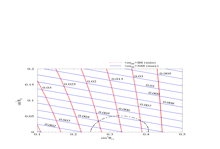
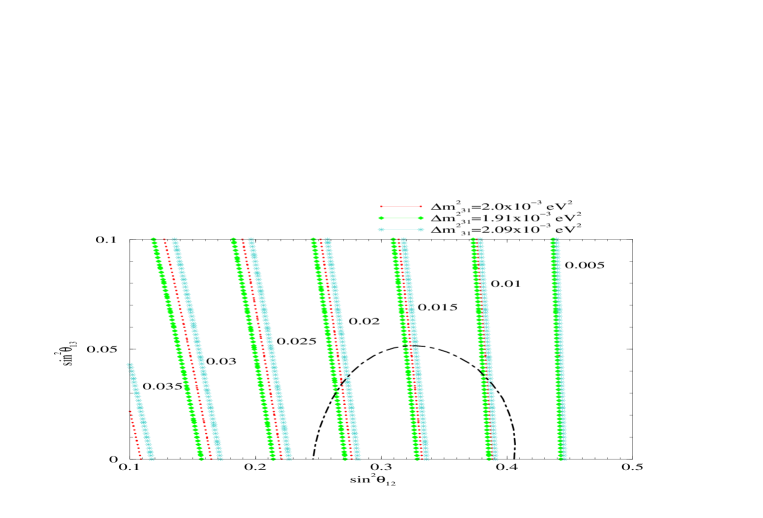
Figure 1: Lines of constant maximum value of $\langle m\rangle$ (in eV) for the NH scheme ($\mbox{$\langle m\rangle$}^{\rm NH}_{\rm max}$) and of constant minimum value of $\langle m\rangle$ for the IH scheme ($\mbox{$\langle m\rangle$}^{\rm IH}_{\rm min}$).

Figure 2: Lines of constant minimal value of $\langle m\rangle$ (in eV) in the IH case ($\mbox{$\langle m\rangle$}^{\rm IH}_{\rm min}$) for different $\Delta m^{2}_{31}$.

We present in Figure 2 the lines of constant maximal and minimal $\langle m\rangle$ for the cases of NH and IH, respectively, in the $\sin^{2}\theta_{12}-\sin^{2}\theta_{13}$ plane. We fixed the values of $\Delta m^{2}_{31}=0.002$ eV² and $\Delta m^{2}_{21}=8\times 10^{-5}$ eV². The dotted (red) lines show the lines of constant minimum value of $\langle m\rangle$ for the IH scheme ($\mbox{$\langle m\rangle$}^{\rm IH}_{\rm min}$) and the solid (blue) lines give the lines of constant maximum value of $\langle m\rangle$ for the NH scheme ($\mbox{$\langle m\rangle$}^{\rm NH}_{\rm max}$). The Figure illustrates the well–known fact that $\mbox{$\langle m\rangle$}^{\rm IH}_{\rm min}$ has a strong $\sin^{2}\theta_{12}$ dependence, while $\mbox{$\langle m\rangle$}^{\rm NH}_{\rm min}$ depends on both $\sin^{2}\theta_{12}$ and $\sin^{2}\theta_{13}$. Also shown by the dot–dashed (black) line on the Figure are the current allowed values of $\sin^{2}\theta_{12}$ and $\sin^{2}\theta_{13}$ at the 3$\sigma$ level, obtained from a 2 parameter fit of the global oscillation data [10]. As an example, one can see from the plot that if we know that the mass ordering is normal and assume that the smallest neutrino mass is negligible, values of the effective mass larger than roughly 0.0053 eV are incompatible with the currently allowed values of $\sin^{2}\theta_{12}$ and $\sin^{2}\theta_{13}$. The same would be the case when we know that the mass ordering is inverted, assume that the smallest neutrino mass is negligible and the effective mass is larger (or smaller) than 0.023 (0.008) eV.

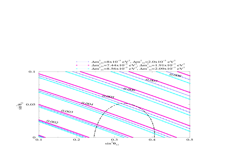
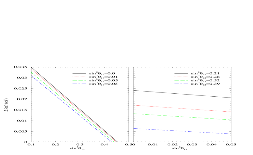
Figure 3: Lines of constant maximal value of $\langle m\rangle$ (in eV) in the NH case ($\mbox{$\langle m\rangle$}^{\rm NH}_{\rm max}$) for different $\Delta m^{2}_{21}$.

Figure 4: The difference between the minimal value of $\langle m\rangle$ for IH and the maximal value of $\langle m\rangle$ for NH, $\mbox{$\langle m\rangle$}^{\rm IH}_{\rm min}-\mbox{$\langle m\rangle$}^{\rm NH}_{\rm max}$, as a function of $\sin^{2}\theta_{12}$ (left–hand panel) and $\sin^{2}\theta_{13}$ (right–hand panel).

We can see from Eqs. (16) and (17) that the maximal and minimal values of $\langle m\rangle$ are crucially dependent on the values of the mass squared differences, especially on $\Delta m^{2}_{31}$. Since we are talking about a future measurement of the $0\mbox{$\nu\beta\beta$}$ signal, we take the expected futuristic uncertainties mentioned in Section 2 on $\Delta m^{2}_{31}$ and $\Delta m^{2}_{21}$ to plot the iso–range of $\mbox{$\langle m\rangle$}^{\rm IH}_{\rm min}$ and $\mbox{$\langle m\rangle$}^{\rm NH}_{\rm max}$ in Figures 2 and 4. We can see clearly from the Figures that the uncertainty on the predicted value of $\langle m\rangle$ due to the uncertainty in the value of $\Delta m^{2}_{31}$ and $\Delta m^{2}_{21}$ would become very small in the next ten years. Therefore, in what follows, we will keep $\Delta m^{2}_{31}$ and $\Delta m^{2}_{21}$ fixed at $\Delta m^{2}_{31}=0.002$ eV² and $\Delta m^{2}_{21}=8\times 10^{-5}$ eV².

Any future positive signal for $0\mbox{$\nu\beta\beta$}$ will be able to distinguish the IH scheme from the NH scheme if the measured value of $\langle m\rangle$ would be such that it could be explained by the predicted $\langle m\rangle$ for just one of the schemes and not the other. In other words, if the difference between the predicted values for $\langle m\rangle$ for the IH scheme and the NH scheme is larger than the error in the measured value of $\langle m\rangle$, then it would be possible (assuming that the smallest neutrino mass is negligible) to experimentally find the neutrino mass hierarchy from a measurement of $0\mbox{$\nu\beta\beta$}$. We therefore show the difference in the predicted value of $\langle m\rangle$ for the two schemes,

$$\Delta\mbox{$\langle m\rangle$}=\mbox{$\langle m\rangle$}^{\rm IH}_{\rm min}-\mbox{$\langle m\rangle$}^{\rm NH}_{\rm max}~{},$$ (22)

in left–hand panel of Figure 4 as a function of $\sin^{2}\theta_{12}$ for 4 fixed values of $\sin^{2}\theta_{13}$ and in right–hand panel of Figure 4 as a function of $\sin^{2}\theta_{13}$ for 4 fixed values of $\sin^{2}\theta_{12}$. We see that $\Delta\mbox{$\langle m\rangle$}$ displays a strong dependence on $\sin^{2}\theta_{12}$, whereas the dependence on $\sin^{2}\theta_{13}$ is rather moderate. In fact, it holds that

$$\Delta\mbox{$\langle m\rangle$}=\frac{\sqrt{\mbox{$\Delta m^{2}_{\rm A}$}}\,\cos^{2}\theta_{13}}{1+\tan^{2}\theta_{12}}\left(1-\tan^{2}\theta_{12}\,\left(1+R+\tan^{2}\theta_{13}\right)-\tan^{2}\theta_{13}\right)~{},$$ (23)

where $R$ is the ratio of the solar and atmospheric $\Delta m^{2}$ defined in Eq. (15). Figure 4 and Eq. (23) demonstrate the well–known fact that distinguishing the normal and inverted hierarchy is easier for smaller values of $\sin^{2}\theta_{12}$. The values of $\Delta\mbox{$\langle m\rangle$}$, which are of the order 0.01 eV, represent a value of the maximal experimental uncertainty which an experiment should have in order to be able to distinguish NH from IH.

Up to here we neglected the complications which arise from the nuclear matrix elements (NME) involved in the calculation of the rate of 0$\nu\beta\beta$. There is neither a consensus in the literature on how large this uncertainty is, nor if there really is a large uncertainty at all [67]. Let us therefore take a conservative point of view and analyze the situation as a function of the NME uncertainty. If there is indeed no problem with the NME, the statements given up to this point apply.

Given the possibility of large uncertainties on the values of the nuclear matrix elements, it is plausible to ask if one could possibly extract the true hierarchy of neutrino masses from a positive signal for $0\mbox{$\nu\beta\beta$}$ in the future. To that end, we look for the difference between $\mbox{$\langle m\rangle$}^{\rm IH}_{\rm min}$ and $\mbox{$\langle m\rangle$}^{\rm NH}_{\rm max}$ after including the uncertainties coming from the nuclear matrix elements. A way to perform such an analysis has been developed in [16], and here we follow a very similar approach: in order to parametrize the uncertainty coming from the nuclear matrix elements, we define the $0\mbox{$\nu\beta\beta$}$ decay rate $\Gamma$ measured in any experiment such that

$$\sqrt{\Gamma}=x\,\mbox{$\langle m\rangle$}~{},$$ (24)

where $x$ contains all other factors involved in the $0\mbox{$\nu\beta\beta$}$ decay, including the NME. Thus for any measured $\Gamma$ the measured value of $\langle m\rangle$ would be

$$\mbox{$\langle m\rangle$}_{\rm measured}=\sqrt{\Gamma}/x~{}.$$ (25)

If $y$ is the smallest possible value for $x$, and if we assume that the uncertainty on $x$ originates solely from the uncertainty on the NME and is a factor of $z$ (with $z>1$), then the range of $x$ is given by $y<x<z\,y$. Therefore, the uncertainty on the measured value of $\langle m\rangle$ that we have due to the uncertainty on the NME is given by

$$\Delta\mbox{$\langle m\rangle$}_{\rm measured}=\frac{z-1}{z+1}~{}.$$ (26)

In order to be able to experimentally distinguish IH from NH with the help of a $0\mbox{$\nu\beta\beta$}$ measurement, we must have $\mbox{$\langle m\rangle$}^{\rm IH}_{\rm min}>\mbox{$\langle m\rangle$}^{\rm NH}_{\rm max}$ after including the uncertainty from the NME. Thus we need the condition

$$\mbox{$\langle m\rangle$}^{\rm IH}_{\rm min}-z\,\mbox{$\langle m\rangle$}^{\rm NH}_{\rm max}>0$$ (27)

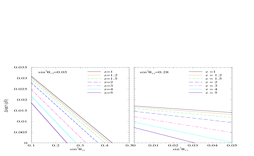
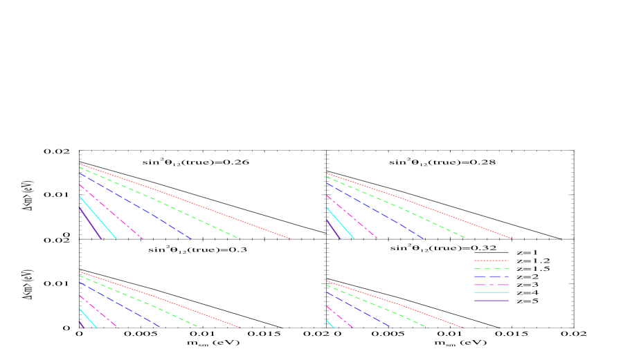
Figure 5: The difference between the minimal value of $\langle m\rangle$ for IH and the maximal value of $\langle m\rangle$ for NH times the NME uncertainty, $\mbox{$\langle m\rangle$}^{\rm IH}_{\rm min}-z\,\mbox{$\langle m\rangle$}^{\rm NH}_{\rm max}$, as a function of $\sin^{2}\theta_{13}$ for different $z$ and $\sin^{2}\theta_{12}=0.28$ (left–hand panel) and $\sin^{2}\theta_{13}$ (right–hand panel).

Figure 6: The difference between the minimal value of $\langle m\rangle$ for IH and the maximal value of $\langle m\rangle$ for NH, $\mbox{$\langle m\rangle$}^{\rm IH}_{\rm min}-\mbox{$\langle m\rangle$}^{\rm NH}_{\rm max}$, as a function of the smallest neutrino mass $m_{\rm sm}$. The 4 panels are for 4 assumed “true” values of $\sin^{2}\theta_{12}$. The values of $\sin^{2}\theta_{12}$ are allowed to vary within 6% of the assumed true value, while $\sin^{2}\theta_{13}$ is allowed to vary between $0$ and $0.0025$.

to ascertain the neutrino mass hierarchy. In the left and right panel of Figure 6 we plot the difference $\mbox{$\langle m\rangle$}^{\rm IH}_{\rm min}-z\,\mbox{$\langle m\rangle$}^{\rm NH}_{\rm max}$ predicted as a function of $\sin^{2}\theta_{12}$ and $\sin^{2}\theta_{13}$, respectively, including the uncertainty coming from the NME. We show the plots assuming a range of values for the NME uncertainty $z$. As a function of $\sin^{2}\theta_{12}$ the quantity $\mbox{$\langle m\rangle$}^{\rm IH}_{\rm min}-z\,\mbox{$\langle m\rangle$}^{\rm NH}_{\rm max}$ shows a similar behavior as for no uncertainty in the NME. The dependence on $\sin^{2}\theta_{13}$ is rather weak for small $z$, but becomes larger with increasing $z$. From Figure 6 one can read of the maximal experimental uncertainty for a given $z$, $\sin^{2}\theta_{13}$ and $\sin^{2}\theta_{12}$ for which one could still be able to distinguish the mass hierarchy. For instance, taking $\sin^{2}\theta_{13}$ close to its current limit and assuming $z=2$ and $\sin^{2}\theta_{12}=0.3$, we have $\mbox{$\langle m\rangle$}^{\rm IH}_{\rm min}-z\,\mbox{$\langle m\rangle$}^{\rm NH}_{\rm max}\simeq 0.01$ eV and the experimental uncertainty should not be larger than this value. For zero $\theta_{13}$ this value becomes larger by roughly $40\%$.

Up to now we considered the case of the smallest mass $m_{\rm sm}$ being zero, which would correspond to the neutrino mass matrix having a zero determinant, clearly a rather limited and special case. For a given set of oscillation parameters and the nuclear matrix elements uncertainty, it would be possible to distinguish between the NH and IH in a $0\nu\beta\beta$ experiment only if $m_{\rm sm}$ is less than a certain value. It is interesting to examine up to which values of the lightest neutrino mass one can distinguish NH from IH. Toward this exercise, we plot in Figure 6 the difference between the minimal value of $\langle m\rangle$ for IH and the maximal value of $\langle m\rangle$ for NH, $\mbox{$\langle m\rangle$}^{\rm IH}_{\rm min}-\mbox{$\langle m\rangle$}^{\rm NH}_{\rm max}$, as a function of the smallest neutrino mass $m_{\rm sm}$. The NME uncertainty is also included in the analysis. For each of the 4 panels we assumed a certain “true” value of $\sin^{2}\theta_{12}$ with an optimistic uncertainty of 6% [41, 57]. For $\sin^{2}\theta_{13}$ we assumed that no positive signal is observed in any of the forthcoming experiments in the next ten years. Thus we allowed it to vary within $0$ and $0.0025$ [42]. We see from the Figure that for $\sin^{2}\theta_{12}=0.3$ for example, when $z=1.5$ ($z=1$, viz. no NME uncertainty) and $\Delta\mbox{$\langle m\rangle$}=0.01$ eV, we can distinguish NH from IH if $m_{\rm sm}$ is smaller than 0.002 (0.004) eV. Of course, the value of $\Delta\mbox{$\langle m\rangle$}$ obtained like this is again an upper limit on the experimental uncertainty which would still allow distinguishing NH from IH for a non–zero smallest mass. If $\sin^{2}\theta_{12}=0.26$ the situation looks more promising. For the same value of $\Delta\mbox{$\langle m\rangle$}=0.01$ eV we can distinguish NH from IH if $m_{\rm sm}$ is smaller than 0.005 (0.01) eV if $z=1.5$ ($z=1$). Other cases are easily read off Figure 6.

For a larger uncertainty in the value of $\sin^{2}\theta_{12}$ and/or for a larger true value of $\sin^{2}\theta_{13}$, the chances of distinguishing the IH from NH become worse and in addition only work for very small values of $m_{sm}$.

We see however that in principle values of $m_{\rm sm}$ up to $\sim 0.01$ eV are allowed in order to distinguish the normal from the inverted neutrino mass hierarchy.

4 Limit on the Neutrino Mass

Another interesting aspect of neutrinoless double beta decay is the possibility to set a limit on the absolute scale of the neutrino mass. The current upper value for the effective mass is somewhere between 0.3 and 1 eV, where this range of course has its origin in the NME uncertainty. The indicated values correspond to the QD mass spectrum, on which we wish to focus in this Section. As indicated in Section 3, for a given common mass scale $m_{0}$, the lowest possible effective mass can be written as

$$\mbox{$\langle m\rangle$}^{\rm QD}_{\min}=m_{0}\,\left(|U_{e1}|^{2}-|U_{e2}|^{2}-|U_{e3}|^{2}\right)=\frac{1-\tan^{2}\theta_{12}-2\,|U_{e3}|^{2}}{1+\tan^{2}\theta_{12}}~{}.$$ (28)

Hence, having a limit on the effective mass at hand, we can translate it into a limit on the neutrino mass. We write the experimental limit as

$$\mbox{$\langle m\rangle$}^{\rm exp}=z\,\mbox{$\langle m\rangle$}_{\min}^{\rm exp}~{},$$ (29)

where $\mbox{$\langle m\rangle$}_{\min}^{\rm exp}$ is defined as the limit on $\langle m\rangle$ obtained by using the largest available NME and $z\geq 1$ encodes again the NME uncertainty. Then, the limit on the neutrino mass reads

$$m_{0}\leq z\,\mbox{$\langle m\rangle$}_{\min}^{\rm exp}\,\frac{1+\tan^{2}\theta_{12}}{1-\tan^{2}\theta_{12}-2\,|U_{e3}|^{2}}\equiv z\,\mbox{$\langle m\rangle$}_{\min}^{\rm exp}\,f(\theta_{12},\theta_{13})~{}.$$ (30)

We have introduced here a function $f(\theta_{12},\theta_{13})$ in this expression, which separates the information available from neutrino oscillation experiments from the information coming from 0$\nu\beta\beta$ and $m_{0}$. We think that this formulation might be helpful in understanding how neutrinoless double beta decay and the absolute neutrino mass scale are related. Currently the uncertainty on $f(\theta_{12},\theta_{13})$ is around 50%, $1.9<f(\theta_{12},\theta_{13})<5.6$. It is expected to reduce to $\sim$ 21%($\sim$ 9) % at $3\sigma$ if a low energy $pp$ solar neutrino experiment (reactor experiment at the survival probability minimum) would be built. The uncertainty depends only little on the value of $\theta_{13}$. From the current limit on the effective mass, $\mbox{$\langle m\rangle$}\leq 0.35\,z$ eV, with the accepted value of $z\simeq 3$ for ⁷⁶Ge (see [20]), and our current knowledge of $f(\theta_{12},\theta_{13})$, we can set a limit on $m_{0}$ of 5.6 eV, clearly weaker than the limit from tritium experiments. Only for close to vanishing NME uncertainty (i.e., $z=1$) we can reach values of $m_{0}\mathrel{\hbox to0.0pt{\raise 2.20013pt\hbox{$<$}\hss}{\lower 2.20013pt\hbox{$\sim$}}}2$ eV which are then comparable to ones from direct searches.

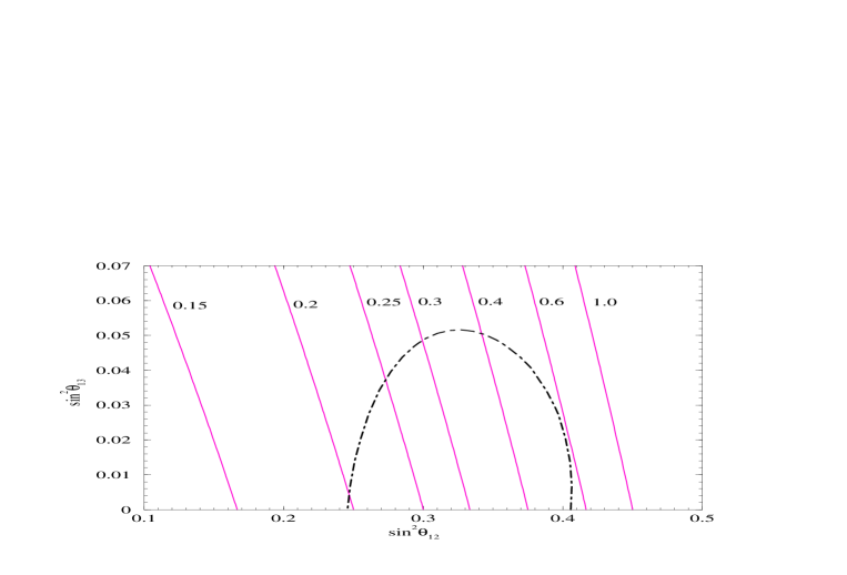
Figure 7: The lines of constant $m_{0}$ in the $\sin^{2}\theta_{12}-\sin^{2}\theta_{13}$ plane, predicted for a QD mass spectrum. Also shown is the current $3\sigma$ allowed region in $\sin^{2}\theta_{12}$ and $\sin^{2}\theta_{13}$.

In Figure 7 we show the iso–contours of $m_{0}$ predicted for the QD mass spectrum (cf. Eq. (30)) in the $\sin^{2}\theta_{12}-\sin^{2}\theta_{13}$ plane. For each of the iso–contours we have assumed an illustrative value of $z\,\mbox{$\langle m\rangle$}_{\min}^{\rm exp}=0.1$ eV. Also shown is the current 3$\sigma$ allowed area of $\sin^{2}\theta_{12}$ and $\sin^{2}\theta_{13}$. From the Figure we can see that for a measured value of $z\,\mbox{$\langle m\rangle$}_{\min}^{\rm exp}=0.1$ eV, the constraint on the common mass scale for a QD spectrum would be: $0.2~{}{\rm eV}\ \raisebox{-1.72218pt}{\hbox to0.0pt{$\sim$\hss}}\raisebox{1.72218pt}{$<$}\ m_{0}\ \raisebox{-1.72218pt}{\hbox to0.0pt{$\sim$\hss}}\raisebox{1.72218pt}{$<$}\ 0.6$ eV. For any other measured value of $z\,\mbox{$\langle m\rangle$}_{\min}^{\rm exp}$ corresponding to a QD mass scheme, we can obtain the corresponding constraints on $m_{0}$ by scaling the above limit suitably, i.e., for $z\,\mbox{$\langle m\rangle$}_{\min}^{\rm exp}=0.2$ eV we would have $0.4~{}{\rm eV}\ \raisebox{-1.72218pt}{\hbox to0.0pt{$\sim$\hss}}\raisebox{1.72218pt}{$<$}\ m_{0}\ \raisebox{-1.72218pt}{\hbox to0.0pt{$\sim$\hss}}\raisebox{1.72218pt}{$<$}\ 1.2$ eV. The limits on $m_{0}$ given above are of course with our existing knowledge about $\theta_{12}$ and $\theta_{13}$. With reduction of the range of allowed values of $\theta_{12}$ and $\theta_{13}$, especially $\theta_{12}$, the constraints on $m_{0}$ are expected to reduce substantially, as discussed above. For instance, if $f(\theta_{12},\theta_{13})$ was known with an uncertainty of $20\%$, say $2.7<f(\theta_{12},\theta_{13})<4.0$, then we would have for $z\,\mbox{$\langle m\rangle$}_{\min}^{\rm exp}=0.1~{}(0.2)$ eV that $0.3~{}{\rm eV}\ \raisebox{-1.72218pt}{\hbox to0.0pt{$\sim$\hss}}\raisebox{1.72218pt}{$<$}\ m_{0}\ \raisebox{-1.72218pt}{\hbox to0.0pt{$\sim$\hss}}\raisebox{1.72218pt}{$<$}\ 0.4$ eV ($0.6~{}{\rm eV}\ \raisebox{-1.72218pt}{\hbox to0.0pt{$\sim$\hss}}\raisebox{1.72218pt}{$<$}\ m_{0}\ \raisebox{-1.72218pt}{\hbox to0.0pt{$\sim$\hss}}\raisebox{1.72218pt}{$<$}\ 0.8$ eV). Of course, if we have no signal for 0$\nu\beta\beta$, but just an upper limit on $z\,\mbox{$\langle m\rangle$}_{\min}$, we have no longer an allowed range on $m_{0}$, but an upper limit corresponding to the largest value in the range. From the examples given above, one can note that for the QD mass spectrum, a measurement or a better constraint on $\langle m\rangle$ will lead to a stronger limit on the absolute neutrino mass scale compared to the current limit from direct kinematical searches.

5 Implications of a Vanishing effective Mass

It is well–known that not only a measurement but also a non–measurement of neutrinoless double beta decay has significant influence on our knowledge of the unknown neutrino parameters. In this Section we wish to discuss a rarely studied subject, namely the impact that a very small upper limit on $\langle m\rangle$ would have. An exactly vanishing $\langle m\rangle$ would correspond to a texture zero in the neutrino mass matrix in the charged lepton basis – certainly an interesting feature. However, to prove/observe an exactly vanishing effective mass is a formidable task.

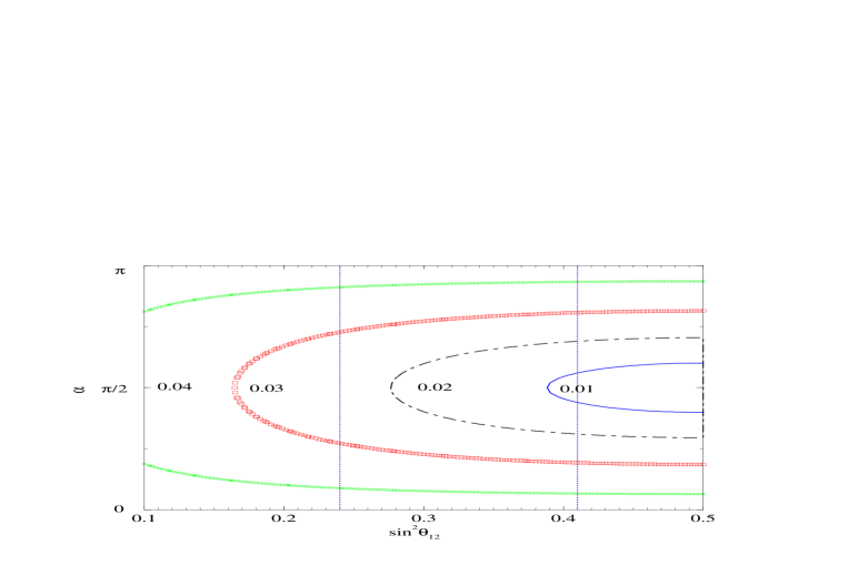
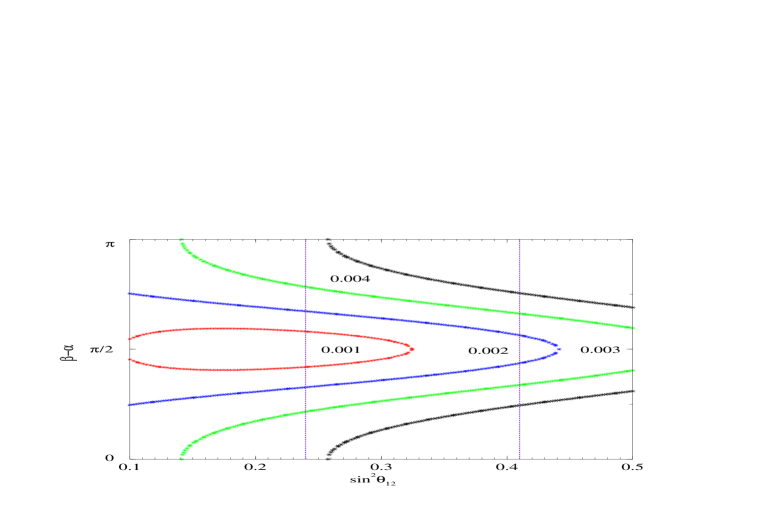
Figure 8: Allowed values of $\sin^{2}\theta_{12}$ and the Majorana phase $\alpha$ for a small upper limit on $\langle m\rangle$ (in eV) in case of IH. The dotted lines show the current $3\sigma$ limit on $\sin^{2}\theta_{12}$. The allowed areas are to the right of the respective curves.

Figure 9: Allowed values of $\sin^{2}\theta_{12}$ and the Majorana phase combination $\beta-\alpha$ for a small upper limit on $\langle m\rangle$ (in eV) in case of NH. The dotted lines show the current $3\sigma$ limit on $\sin^{2}\theta_{12}$. The allowed areas are to the left of the respective curves.

In case of an inverted hierarchy we know that there is a lower limit of $\langle m\rangle$ which is — when using current $3\sigma$ values of the oscillation parameters — given by roughly 0.006 eV, see Eq. (20). Let us assume that neutrinos are Majorana particles, have an inverted ordering and that the effective mass takes has an upper limit of order 0.01 eV. This is a situation which might arise if we know from some other independent experiment that sgn$(\mbox{$\Delta m^{2}_{\rm A}$})=-1$ and the next generation 0$\nu\beta\beta$–experiments do not find a signal corresponding to a non–vanishing $\langle m\rangle$, but give an upper limit on $\langle m\rangle$ still above the theoretical limit $\mbox{$\langle m\rangle$}_{\rm min}^{\rm IH}$. Then we can infer from Eq. (17) the values of $\sin^{2}\theta_{12}$ and the Majorana phase $\alpha$ which are still compatible with the data. In Fig. 9 we display the result for an experimental upper limit on $\langle m\rangle$ of 0.04, 0.03, 0.02, 0.01 eV, taking $m_{3}=0$, $\theta_{13}=0$ and $\Delta m^{2}_{31}=0.002$ eV². We checked that the results are rather stable when we depart from these values within their current uncertainty. The current $3\sigma$ values of $\sin^{2}\theta_{12}$ are also indicated in the Figure. Allowed is the area to the right of the respective curves. For instance, if $\mbox{$\langle m\rangle$}<0.02$ eV and $\sin^{2}\theta_{12}=0.3$ then $\alpha$ has to lie between 1.2 and 1.9, or $\alpha\simeq\pi/2\pm 0.4$. Alternatively, if $\mbox{$\langle m\rangle$}<0.02$ eV and $\sin^{2}\theta_{12}<0.28$, then the IH case is ruled out.

Figure 9 shows a similar analysis for the case of NH with a smallest mass $m_{1}=0$. In our parametrization, as can be seen from Eq. (16), it is the combination $\beta-\alpha$ which governs the destructive interference which leads to very small or zero $\langle m\rangle$. We took very small upper limits on $\langle m\rangle$ of 0.004, 0.003, 0.002 and 0.001 eV (hence this discussion will not become realistic within the next 10 years) and chose $m_{1}=0$, $\sin^{2}\theta_{13}=0.04$ $\Delta m^{2}_{21}=8\times 10^{-5}$ eV² and $\Delta m^{2}_{31}=0.002$ eV². Note that for very small values of $\theta_{13}$, corresponding to $\sin^{2}\theta_{13}\ll R\,\sin^{2}\theta_{12}\sim 0.01$, the dependence on this combination of phases drops. In this part of the Figure it is the left of the respective curve which is allowed. For instance, for $\mbox{$\langle m\rangle$}\mathrel{\hbox to0.0pt{\raise 2.20013pt\hbox{$<$}\hss}{\lower 2.20013pt\hbox{$\sim$}}}$ 0.002 eV and a rather large value of $\sin^{2}\theta_{12}=0.4$ the phases have to be very close to $\pi/2$, namely $\beta-\alpha\simeq\pi/2\pm 0.2$. Alternatively, if $\mbox{$\langle m\rangle$}<0.001$ eV and $\sin^{2}\theta_{12}>0.33$, then the NH case is ruled out.

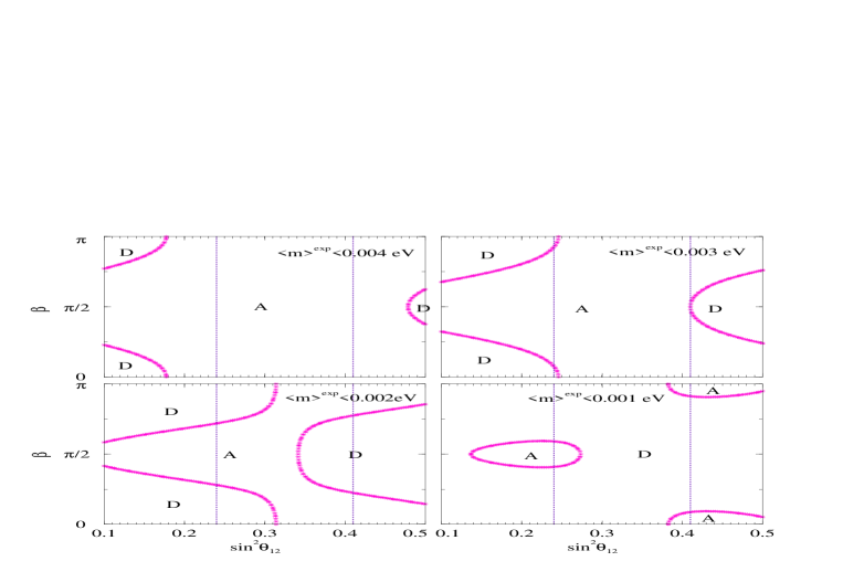
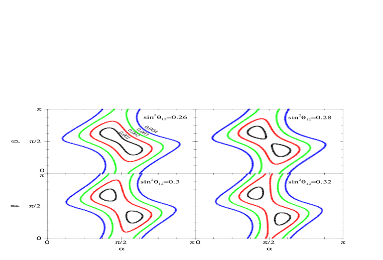
Figure 10: Allowed values of $\sin^{2}\theta_{12}$ and the Majorana phase $\beta$ for a smallest neutrino mass of $m_{1}=0.005$ eV in case of NH for 4 different assumed upper limits on $\langle m\rangle$ and $\alpha=\pi/2$. The dotted lines show the current $3\sigma$ limit on $\sin^{2}\theta_{12}$. The allowed (disallowed) areas are marked with A (D).

Figure 11: Allowed values of the Majorana phases $\alpha$ and $\beta$ for a smallest neutrino mass of $m_{1}=0.005$ eV in case of NH for 4 different assumed upper limits on $\langle m\rangle$. The 4 panels correspond to 4 different true values of $\sin^{2}\theta_{12}$ shown on the Figure. Allowed are the areas within the respective curves.

As mentioned earlier in Section 3 we note here that in the case of NH, $\langle m\rangle$ could have a sizable dependence on the smallest neutrino mass state $m_{1}$. We plot therefore in Fig. 11 the same as in Fig. 9 but for a smallest neutrino mass of $m_{1}=0.005$ eV. We took again $\sin^{2}\theta_{13}=0.04$, $\Delta m^{2}_{21}=8\times 10^{-5}$ eV² and $\Delta m^{2}_{31}=0.002$ eV² and chose the same four upper limits on $\langle m\rangle$ as above. With a non–vanishing $m_{1}$ Eq. (16) is modified to

$$\mbox{$\langle m\rangle$}\simeq\left|m_{1}\,\cos^{2}\theta_{12}\,\cos^{2}\theta_{13}+\sqrt{m_{1}^{2}+\mbox{$\Delta m^{2}_{\odot}$}}\,\sin^{2}\theta_{12}\,\cos^{2}\theta_{13}\,e^{2i\alpha}+\sqrt{\mbox{$\Delta m^{2}_{\rm A}$}}\,\sin^{2}\theta_{13}\,e^{2i\beta}\right|~{}$$ (31)

and thus it is no longer $\beta-\alpha$ but both $\alpha$ and $\beta$ which play a role. In Figure 11 we fixed $\alpha=\pi/2$ which gives a negative sign for the second term in Eq. (31). We indicate the allowed (disallowed) values of the parameter regions in the Figure with A (D). If $\mbox{$\langle m\rangle$}<0.004$ eV and $\mbox{$\langle m\rangle$}<0.003$ eV the disallowed areas are already outside the currently allowed $3\sigma$ region of $\sin^{2}\theta_{12}$ for $\alpha$ fixed at $\pi/2$. To show the dependence of our results on $\alpha$, we plot in Figure 11 the allowed areas in the $\alpha$–$\beta$ plane for four different fixed values of $\sin^{2}\theta_{12}$, keeping $\sin^{2}\theta_{13}$ fixed at 0.04 and for $m_{1}=0.005$ eV. Allowed are the areas within the respective curves.

An interesting aspect is when $\theta_{13}$ vanishes but $m_{1}$ is non–zero. Then the effective mass is a function of the phase $\alpha$ alone:

$$\mbox{$\langle m\rangle$}\simeq\left|m_{1}\,\cos^{2}\theta_{12}+\sqrt{m_{1}^{2}+\mbox{$\Delta m^{2}_{\odot}$}}\,\sin^{2}\theta_{12}\,e^{2i\alpha}\right|~{}.$$ (32)

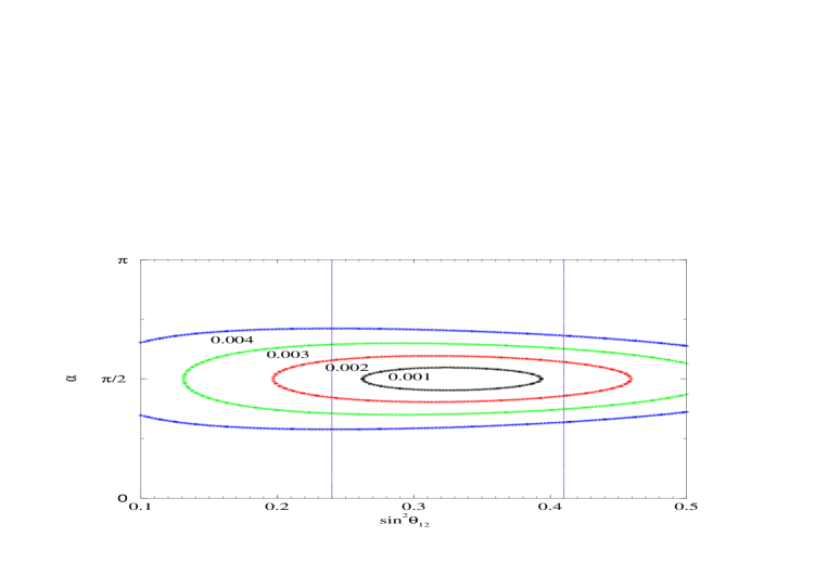
Figure 12: Allowed values of the Majorana phase $\alpha$ and $\sin^{2}\theta_{12}$ for NH for $\sin^{2}\theta_{13}=0$ and with a non–zero smallest neutrino mass of $m_{1}=0.005$ eV in case of NH for 4 different assumed upper limits on $\langle m\rangle$. The dotted lines show the current $3\sigma$ limit on $\sin^{2}\theta_{12}$. Allowed are the areas within the respective curves.

In Figure 12 we show the areas in the $\sin^{2}\theta_{12}$–$\alpha$ plane that would be allowed if we had an upper limit on $\langle m\rangle$ of 0.001 eV (black line), 0.002 eV (red line), 0.003 eV (green line) and 0.004 eV (blue line). The areas outside the closed curves would be disallowed. We can see that for a limit of $\langle m\rangle$=0.001 eV, all values of $\alpha$ could be possible while for $\langle m\rangle$=0.004 eV, only the range $\pi/2\pm 0.67$ is allowed. This allowed range of $\alpha$ is not expected to improve with the reduction of the uncertainty on $\sin^{2}\theta_{12}$ since its $\theta_{12}$ dependence, as can be seen from the Figure, is very weak.

For values of the smallest mass of $m_{1}\simeq 0.005$ eV and $\sin^{2}\theta_{12}\simeq 0.3$ both terms in Eq. (32) are of roughly the same magnitude (i.e., $m_{1}\simeq m_{2}$) and we could write

$$\mbox{$\langle m\rangle$}\simeq m_{\rm NH}\,\sqrt{1-\sin^{2}2\theta_{12}\,\sin^{2}\alpha}~{},\mbox{ where }m_{\rm NH}\equiv\sqrt{m_{1}^{2}+\mbox{$\Delta m^{2}_{\odot}$}}\sim 0.01~{}\rm eV.$$

Note the similarity of this equation with Eq. (17) in case of IH.

To sum up, in certain cases it might be possible to significantly constrain the allowed values of the Majorana phases. Moreover, the allowed values of the solar neutrino oscillation parameter $\theta_{12}$ can be comparable to its current known range.

6 Neutrinoless Double Beta Decay, Future Neutrino Oscillation Data and the Identification of the Neutrino Mass Matrix

In this Section we wish to give a summary of typical neutrino mass matrices available in the vast literature. Predictions for and correlations between the neutrino observables are implied by each of the candidates and can be used to distinguish them. In particular, knowledge of the neutrino mass spectrum, $R$, $U_{e3}$, $\theta_{23}$ and of course the effective mass are then very helpful for identifying the correct mass matrix. A complete study of all possibilities is (and maybe can) not performed, however, we feel that the majority of the models will produce at the end of the day a mass matrix which will more or less correspond to one of the examples given here. For instance, there are many symmetries which eventually lead to a $\mu\tau$ symmetric mass matrix [69], see for instance Refs. [70] for some examples. For more models and details we refer to the excellent reviews available [71]. We should remark that for the given examples, unless otherwise stated, the charged lepton mass matrix $m_{\ell}$ is diagonal, i.e., for the matrix $U_{\ell}$ diagonalizing $m_{\ell}m_{\ell}^{\dagger}$ holds that $U_{\ell}=\mathbbm{1}$, and therefore the PMNS matrix is just $U=U_{\ell}^{\dagger}\,U_{\nu}=U_{\nu}$, where $U_{\nu}$ diagonalizes $m_{\nu}$. Further note that most correlations focus on the quantities $\langle m\rangle$, $R$, $\theta_{23}$, $|U_{e3}|$ or $\theta_{12}$. Interplay with the parameters describing $CP$ violation is rarely studied.

Let us focus first on the normal hierarchy, for which there is a very successful and well–known texture, namely [72]

$$m_{\nu}=m_{0}\,\left(\begin{array}[]{ccc}a\,\epsilon^{2}&b\,\epsilon&d\,\epsilon\\[8.5359pt] \cdot&e&f\\[8.5359pt] \cdot&\cdot&g\end{array}\right)~{}.$$ (36)

Here $a,b,d,e,f,g$ are complex parameters of order one and $\epsilon$ is a real and small parameter typically of order of the Cabibbo angle $\lambda\simeq 0.22$. Such a mass matrix preserves at leading order the lepton charge $L_{e}$ and can be obtained already by simple models based on $U(1)$ charges or through sequential right–handed neutrino dominance [73]. A correlation resulting from Eq. (36) is

$$\mbox{$\langle m\rangle$}=c_{1}\,\sqrt{\mbox{$\Delta m^{2}_{\rm A}$}}\,|U_{e3}|^{2}~{}\mbox{ with }~{}|U_{e3}|=c_{2}\,R~{},$$ (37)

where $c_{1,2}$ are functions of the order one parameters and naturally also of order one. With the parameters in the $\mu\tau$ block unspecified, the atmospheric neutrino mixing angle typically deviates sizable from its maximal value $\pi/4$, i.e., $\theta_{23}=\pi/4-c_{3}\,\sqrt{R}$.

The discussion is also possible in the context of $\mu\tau$ symmetric mass matrices [69, 70]. Since their predictions include maximal $\theta_{23}$ and zero $\theta_{13}$, one is interested in breaking schemes of the symmetry. Breaking the symmetry in the $e$ sector of $m_{\nu}$ leads to the same correlation [74] as in Eq. (37) but atmospheric neutrino mixing is much closer to $\pi/4$. On the other hand, breaking the $\mu\tau$ symmetry in the $\mu\tau$ sector of $m_{\nu}$ leads to [74]

$$\mbox{$\langle m\rangle$}\simeq c_{1}\,\sqrt{\mbox{$\Delta m^{2}_{\rm A}$}}\,|U_{e3}|~{},$$ (38)

where $|U_{e3}|$ is now very small, $|U_{e3}|=c_{2}\,R$, and the deviation from maximal atmospheric neutrino mixing is again sizable, i.e., of order $\sqrt{R}$. Another interesting breaking scenario of $\mu\tau$ symmetric mass matrices is when the $e\mu$ element is not identical to, but the complex conjugate of the $e\tau$ element [75]. Then one finds that $U_{e3}\neq 0$ but Re$\,U_{e3}=0$, i.e., there is maximal $CP$ violation with $\delta=\pm\pi/2$. A special case of $\mu\tau$ symmetric mass matrices, for which similar statements will apply, is given when $\tan^{2}\theta_{12}=0.5$, which then corresponds to the so–called tri–bimaximal mixing scheme [76]. “Bimaximal” scenarios [77] with their prediction $\tan^{2}\theta_{12}=1$ typically require contributions from the charged leptons, see below.

Perturbing a zeroth order mass matrix that leads to zero $U_{e3}$ and maximal $\theta_{23}$ with a random matrix containing small entries of the same order $\epsilon$ [78], will lead to a semi–hierarchical mass spectrum (i.e., $m_{2}>m_{1}$ and not $m_{2}\gg m_{1}$) with a somewhat larger $\langle m\rangle$ and also to sizable deviations both from $U_{e3}=0$ and $\theta_{23}=\pi/4$ [78].

Other candidates studied frequently in the literature are minimal models in the sense of having zeros in $m_{\nu}$ [79] or a minimal number of parameters in a see–saw context [80].

Table 2 summarizes our collection of the typical mass matrices for the normal mass hierarchy. Once we know that the neutrino mass spectrum is hierarchical, an information that could be provided by a negative search for 0$\nu\beta\beta$ in future experiments and knowing that sgn$(\Delta m^{2}_{31})=+1$, we can sort out the correct mass matrix when we have precise information on the oscillation parameters.

In case of the inverted hierarchy, summarized in Table 2, the most stable candidate “theory” corresponds to a mass matrix conserving the flavor charge $L_{e}-L_{\mu}-L_{\tau}$ [81]. Such a matrix is given by

$$m_{\nu}=m_{0}\left(\begin{array}[]{ccc}0&\cos\theta&\sin\theta\\[8.5359pt] \cdot&0&0\\[8.5359pt] \cdot&\cdot&0\end{array}\right)~{},$$ (42)

predicting one massless neutrino, zero $\theta_{13}$, zero $\langle m\rangle$, maximal solar neutrino mixing with $\mbox{$\Delta m^{2}_{\odot}$}=0$ and $\theta_{23}=\theta$. Barring extreme fine–tuning, it is impossible to perturb the structure of Eq. (42) such that the measured values of $\theta_{12}$ and $\Delta m^{2}_{\odot}$ are both accommodated in accordance with the data. Typically, after breaking it will hold that $\tan^{2}\theta_{12}\simeq 1\pm R/2$ ($\sin^{2}\theta_{12}\simeq\frac{1}{2}\pm R/4$), whereas experimentally $\sin^{2}\theta_{12}\simeq\frac{1}{2}-\sqrt{R}$ is required. An exception is a see–saw model in which the perturbations at high energy have the same order of magnitude as the terms allowed by the symmetry, see [82]. In that example, $U_{e3}$ and the smallest mass state remain zero. Another way out is to take corrections from the charged lepton sector into account [83]. The matrix $U_{\ell}$, which diagonalizes $m_{\ell}m_{\ell}^{\dagger}$, is multiplied from the left to $U_{\nu}$, which is the matrix diagonalizing $m_{\nu}$ from Eq. (42). The latter has to be perturbed in order to generate a non–zero $\Delta m^{2}_{\odot}$. Given the observation that the deviation from maximal solar neutrino mixing is determined by the Cabibbo angle, i.e., $\pi/4-\theta_{\odot}\simeq\lambda\simeq 0.22\simeq\theta_{C}$ [84], one assumes a CKM–like structure of $U_{\ell}$ [85]. The typical result of the described Ansatz lies in a correlation between the solar neutrino mixing and $U_{e3}$, namely $\sin^{2}\theta_{12}\simeq\frac{1}{2}-\cos\phi\,\cot\theta_{23}\,|U_{e3}|$ , where $\phi$ is a phase appearing in $m_{\nu}$, which can be given by the Dirac phases as measurable in oscillation experiments. This depends however on the breaking in $m_{\nu}$. Nevertheless, both $|U_{e3}|$ and $\tan^{2}\theta_{12}$ are expected to be close to their current upper limits. Assuming minimal breaking in $m_{\nu}$ [83] one can show that there are remarkable correlations between the observables, such as $\mbox{$\langle m\rangle$}\simeq\sqrt{\mbox{$\Delta m^{2}_{\rm A}$}}\,\left|\cos 2\theta_{12}+4i\,J_{CP}/\sin^{2}\theta_{23}\right|$, where $J_{CP}$ is the Jarlskog invariant for $CP$ violating effects in neutrino oscillations, which is proportional to $|U_{e3}|/4$. This represents one of the few examples where the $CP$ phases are part of the predicted correlations, depending however on the details of the model. The correlation $\tan^{2}\theta_{12}\simeq 1-4~{}|U_{e3}|$ is however independent of the breaking in $m_{\nu}$ and relies only on bi–large $U_{\nu}$ [85]. Hence, the two discussed possibilities incorporating $L_{e}-L_{\mu}-L_{\tau}$ predict values for $\langle m\rangle$ of similar size but predict either zero or large $U_{e3}$.

There is another zeroth order scheme for the inverted hierarchy, namely

$$m_{\nu}=m_{0}\left(\begin{array}[]{ccc}1&0&0\\[8.5359pt] \cdot&1/2&1/2\\[8.5359pt] \cdot&\cdot&1/2\end{array}\right)~{}.$$ (46)

Zero $U_{e3}$ and maximal $\theta_{23}$ are predicted and the two leading mass states have the same sign. One can perturb this structure [78] and the result is that both $U_{e3}$ and $\theta_{23}-\pi/4$ are very small quantities, but the effective mass is larger than in case of matrices based on the conservation of $L_{e}-L_{\mu}-L_{\tau}$.

The dependence of $\langle m\rangle$ on $U_{e3}$ goes from none to sizable to little in the three cases discussed, cf. with Table 2. So, if we know that the mass ordering is inverted, i.e., sgn$(\Delta m^{2}_{31})=-1$ and the effective mass is of order $\sqrt{\mbox{$\Delta m^{2}_{\rm A}$}}$, then we basically only have to distinguish between $L_{e}-L_{\mu}-L_{\tau}$ from Eq. (42) and the matrix given in Eq. (46). This can be done by knowing how to close $\langle m\rangle$ is to $\sqrt{\mbox{$\Delta m^{2}_{\rm A}$}}$. More precision data on $U_{e3}$ and $\theta_{23}$ will fix the details of the model.

Now we turn to quasi–degenerate neutrinos. Usually, in such scenarios both the normal and the inverted mass ordering can be accommodated. Typical examples are given in Table 3. There are matrices with two zero entries which are compatible with quasi–degenerate neutrinos and which predict an interesting interplay of observables [79]. Anarchical mass matrices [86] do in general not generate extreme mixing angles and therefore typically result in large deviations from zero $U_{e3}$ and maximal $\theta_{23}$, i.e., of order $R$.

Possibilities to obtain QD neutrinos are models based on flavor democracy [87], of which we quote in Table 3 one interesting recent and typical example [88]. In such models both $U_{\nu}$ and $U_{\ell}$ are required in order to reproduce the neutrino data, resulting in a dependence of the neutrino observables on the charged lepton masses. This makes the predictions also a function of the democracy breaking scenario, therefore somewhat model–dependent. However, the smallness of $|U_{e3}|$ in such models can be attributed to the small ratios of the charged lepton masses.

One can also upgrade a hierarchical mass spectrum (e.g. resulting from sequential dominance) to a quasi–degenerate one by adding a term proportional to the unit matrix (e.g. connected to a $SO(3)$ symmetry) to it [89]. The neutrino mixing angles display approximately the same behavior as in the NH case (i.e., as from Eq. (36)), however, the effective mass is close to the common mass scale, i.e., there is little cancellation in $\langle m\rangle$. Moreover, the larger $m_{0}$ the smaller the phases [89].

Some attention has recently been caught by a model based on the discrete symmetry $A_{4}$ [90]. Applying the most general SUSY threshold corrections to the resulting mass matrix leads to predictions such as very large atmospheric mixing, purely imaginary $U_{e3}$ with an absolute value of order $\sqrt{R}$ and $\mbox{$\langle m\rangle$}=m_{0}$. Similarly, one can use a simple Abelian symmetry corresponding to the conservation of the flavor symmetry $L_{\mu}-L_{\tau}$ [91] and perturb the resulting mass matrix

$$m_{\nu}=m_{0}\left(\begin{array}[]{ccc}\cos\theta&0&0\\[8.5359pt] \cdot&0&\sin\theta\\[8.5359pt] \cdot&\cdot&0\end{array}\right)~{},$$ (50)

to which the $A_{4}$ model corresponds when $\theta=\pi/4$. The deviations from zero $U_{e3}$ and maximal $\theta_{23}$ are small and inverse proportional to $m_{0}^{2}$. Note that interestingly most of the models presented here have $\mbox{$\langle m\rangle$}\simeq m_{0}$, i.e., the mass parameters hopefully measured in direct laboratory searches and in neutrinoless double beta decay experiments should be almost identical.

Another zeroth order scheme for quasi–degenerate neutrinos corresponds to a matrix of the form [92]

$$m_{\nu}=m_{0}\left(\begin{array}[]{ccc}0&-1/\sqrt{2}&1/\sqrt{2}\\[8.5359pt] \cdot&(1+\eta)/2&(1+\eta)/2\\[8.5359pt] \cdot&\cdot&(1+\eta)/2\end{array}\right)~{}.$$ (54)

Exact bimaximal mixing is predicted and breaking of the matrix is also required to generate splittings between the mass states. Similar statements as for the matrix Eq. (42) hold, i.e., without extreme fine–tuning it is impossible to generate deviations from maximal solar neutrino mixing sizable enough not to be in conflict with the data. Hence, the contribution from the charged lepton sector are required, which will lead to similar correlations as for $L_{e}-L_{\mu}-L_{\tau}$ discussed above, such as $\tan^{2}\theta_{12}\simeq 1-4~{}|U_{e3}|$. The correlation between the other observables depends strongly on the breaking. Since however the $ee$ element is zero in Eq. (54), the effective mass is expected to be small, i.e., $\mbox{$\langle m\rangle$}\simeq m_{0}\,\cos 2\theta_{12}$.

Hence, the identification of the mass matrix in case of a QD spectrum can be performed when information also from direct kinematical or from cosmological measurements is available. With the expected future precision data the identification of the mass matrix should also be possible.

To sum up this Section, a complete determination of the all neutrino observables and consequent identification of correlations will be able to discriminate between the various possible models. At least some of the possible candidates will be ruled out. Note finally that the values of the two Majorana phases, whose determination turned out to be an extremely challenging task, is not really required in order to identify the mass matrix.

7 Conclusions

We have analyzed some aspects of the connection between neutrinoless double beta decay, the neutrino mass scale and neutrino oscillation parameters. In particular, we concentrated on the question whether the expected future precision on the oscillation parameters simplifies certain important consequences of a measurement of, or improved upper limit on, 0$\nu\beta\beta$. We first summarized the current situation of the determination of the nine physical parameters of the neutrino mass matrix and the prospects of improving our knowledge about them with future experiments. Then we analyzed how 0$\nu\beta\beta$ can help in distinguishing the normal mass ordering from the inverted one. We included the nuclear matrix element uncertainty in the analysis and pointed attention to the fact that distinguishing NH from IH depends on the value of the smallest neutrino mass $m_{\rm sm}$. We analyzed this point and found that in principle values of $m_{\rm sm}=0.01$ eV are allowed, where of course the issue of the nuclear matrix elements can significantly spoil this possibility.

Then we investigated inasmuch 0$\nu\beta\beta$ can be used to set a limit on the neutrino mass scale $m_{0}$ in case of a quasi–degenerate spectrum. We argued how the information from oscillation data and from 0$\nu\beta\beta$ can be separated. Current limits on $m_{0}$ are weaker than direct ones but can be significantly improved with future 0$\nu\beta\beta$–experiments and more precise knowledge of the oscillation parameters $\sin^{2}\theta_{12}$ and $\sin^{2}\theta_{13}$.

Next we studied the implications of a very small, or even vanishing effective mass. Still insisting that neutrinos are Majorana particles, one can put in this case interesting constraints on parameters, in particular on $\sin^{2}\theta_{12}$ and the Majorana phases.

Finally, we tried to perform a scan through the literature and identified neutrino mass matrices, which tend to arise frequently in many different models. We listed their predictions and correlations and argued how future precision date of the oscillation parameters and information from neutrinoless double beta decay can help to identify the true neutrino mass matrix or at least to sort out many unsuccessful ones.

Acknowledgments

This work was supported by the “Deutsche Forschungsgemeinschaft” in the “Sonderforschungsbereich 375 für Astroteilchenphysik” and under project number RO–2516/3–1 (W.R.) and PPARC grant number PPA/G/O/2002/00479 (S.C.).

Matrix $m_{\nu}/m_{0}$	comments	correlations
$\left(\begin{array}[]{ccc}a\,\epsilon^{2}&b\,\epsilon&d\,\epsilon\\[8.5359pt] \cdot&e&f\\[8.5359pt] \cdot&\cdot&g\end{array}\right)$	$\begin{array}[]{c}{\rm Ref.\ \cite[cite]{[\@@bibref{}{NH1}{}{}]}}\\ {\rm e.g.,simple~{}}U(1),{\rm broken~{}}L_{e}\\ \mbox{sequantial dominance}\end{array}$	$\begin{array}[]{c}\mbox{$\langle m\rangle$}=c_{1}\,\sqrt{\mbox{$\Delta m^{2}_{\rm A}$}}\,|U_{e3}|^{2}\\ |U_{e3}|=c_{2}\,\sqrt{R},~{}\theta_{23}=\frac{\pi}{4}-c_{3}\,\sqrt{R}\\ {\rm normal~{}hierarchy}\end{array}$
$\left(\begin{array}[]{ccc}a\,\epsilon&b\,\epsilon&d\,\epsilon\\[8.5359pt] \cdot&1+f\,\epsilon&1+g\,\epsilon\\[8.5359pt] \cdot&\cdot&1+h\,\epsilon\end{array}\right)$	$\begin{array}[]{c}{\rm Ref.~{}}\cite[cite]{[\@@bibref{}{adg}{}{}]}\\ {\rm perturbed~{}}m_{\nu}^{0}\\ {\rm broken~{}}L_{e}\end{array}$	$\begin{array}[]{c}\mbox{$\langle m\rangle$}=\frac{\sqrt{\Delta m^{2}_{\rm atm}}}{2}\,(1+c_{1}~{}|U_{e3}|)\\ |U_{e3}|=c_{2}\,\sqrt{R},~{}\theta_{23}=\frac{\pi}{4}-c_{3}\,\sqrt{R}\\ {\rm normal~{}ordering~{}}m_{2}>m_{1}\end{array}$
$\left(\begin{array}[]{ccc}a\,\epsilon^{2}&b\,\epsilon&d\,\epsilon\\[8.5359pt] \cdot&1+\epsilon&1\\[8.5359pt] \cdot&\cdot&1+\epsilon\end{array}\right)$	$\begin{array}[]{c}{\rm Ref.\ \cite[cite]{[\@@bibref{}{rabimutau}{}{}]}}\\ \mu\tau~{}{\rm symmetry}\\ {\rm broken~{}in~{}}e~{}{\rm sector}\end{array}$	$\begin{array}[]{c}\mbox{$\langle m\rangle$}=c_{1}\,\sqrt{\mbox{$\Delta m^{2}_{\rm A}$}}\,|U_{e3}|^{2}\\ |U_{e3}|=c_{2}\,\sqrt{R},~{}\theta_{23}=\frac{\pi}{4}-c_{3}\,R\\ {\rm normal~{}hierarchy}\end{array}$
$\left(\begin{array}[]{ccc}a\,\epsilon^{2}&b\,\epsilon&b\,\epsilon\\[8.5359pt] \cdot&1+d\epsilon&1\\[8.5359pt] \cdot&\cdot&1+\epsilon\end{array}\right)$	$\begin{array}[]{c}{\rm Ref.\ \cite[cite]{[\@@bibref{}{rabimutau}{}{}]}}\\ \mu\tau~{}{\rm symmetry}\\ {\rm broken~{}in~{}}\mu\tau~{}{\rm sector}\end{array}$	$\begin{array}[]{c}\mbox{$\langle m\rangle$}=c_{1}\,\sqrt{\mbox{$\Delta m^{2}_{\rm A}$}}\,|U_{e3}|\\ |U_{e3}|=c_{2}\,R,~{}\theta_{23}=\frac{\pi}{4}-c_{3}\,\sqrt{R}\\ {\rm normal~{}hierarchy}\end{array}$
$\left(\begin{array}[]{ccc}0&0&\epsilon\\[8.5359pt] \cdot&a&b\\[8.5359pt] \cdot&\cdot&d\end{array}\right)$	$\begin{array}[]{c}{\rm Ref.\ \cite[cite]{[\@@bibref{}{2zeros}{}{}]}}\\ \mbox{2 zeros}\\ \mbox{very similar to }m_{ee}=m_{e\tau}=0\end{array}$	$\begin{array}[]{c}\mbox{$\langle m\rangle$}=0\\ |U_{e3}|=\sqrt{\frac{R}{\cos 2\theta_{12}}}\,\frac{\sin 2\theta_{12}}{2\,\tan\theta_{23}}\\ {\rm normal~{}hierarchy}\end{array}$
$\left(\begin{array}[]{ccc}a^{2}\,\epsilon&a\sqrt{1-a^{2}}\,\epsilon&0\\[8.5359pt] \cdot&b^{2}+(1-a^{2})\,\epsilon&b\,\sqrt{1-b^{2}}\\[8.5359pt] \cdot&\cdot&1-b^{2}\end{array}\right)$	$\begin{array}[]{c}{\rm Ref.\ \cite[cite]{[\@@bibref{}{minSS}{}{}]}}\\ \mbox{minimal see--saw }\end{array}$	$\begin{array}[]{c}\mbox{$\langle m\rangle$}=\sqrt{\mbox{$\Delta m^{2}_{\odot}$}}\,\sin^{2}\theta_{12}\\ |U_{e3}|=\sqrt{R}/2\,\sin 2\theta_{12}\,\tan\theta_{23}\\ {\rm normal~{}hierarchy},~{}m_{1}=0\end{array}$

Table 1: Typical and popular neutrino mass matrices predicting the normal mass hierarchy. Given are some comments about their origin and order of magnitude predictions for correlations between the observables. The parameter $\epsilon$ is usually small, i.e., mostly of order $\lambda\simeq 0.22$ and the parameters $a,b,d,e,f,c_{1,2,3}$ are of order one.

Matrix $m_{\nu}/m_{0}$	comments	correlations
$\left(\begin{array}[]{ccc}1+a\,\epsilon&b\,\epsilon&d\,\epsilon\\[8.5359pt] \cdot&1/2+f\,\epsilon&1/2+g\,\epsilon\\[8.5359pt] \cdot&\cdot&1/2+h\,\epsilon\end{array}\right)$	$\begin{array}[]{c}{\rm Ref.\ \cite[cite]{[\@@bibref{}{adg}{}{}]}}\\ {\rm perturbed~{}}m_{\nu}^{0}\end{array}$	$\begin{array}[]{c}\mbox{$\langle m\rangle$}=\sqrt{\mbox{$\Delta m^{2}_{\rm A}$}}\,(1+c_{1}\,|U_{e3}|)\\ |U_{e3}|=c_{2}\,R,~{}\theta_{23}=\frac{\pi}{4}-c_{3}\,R\\ {\rm inverted~{}hierarchy}\end{array}$
$\left(\begin{array}[]{ccc}0&a&b\\[8.5359pt] \cdot&\epsilon^{2}&0\\[8.5359pt] \cdot&\cdot&0\end{array}\right)$	$\begin{array}[]{c}{\rm Ref.~{}}\cite[cite]{[\@@bibref{}{SP}{}{}]}\\ {\rm broken~{}}L_{e}-L_{\mu}-L_{\tau}\\ {\rm and~{}}U_{\ell}\sim V_{\rm CKM}\end{array}$	$\begin{array}[]{c}\small\mbox{$\langle m\rangle$}=\sqrt{\mbox{$\Delta m^{2}_{\rm A}$}}\,\left|\cos 2\theta_{12}+4i/\sin^{2}\theta_{23}\,J_{CP}\right|\\ \tan^{2}\theta_{12}=1-4\,\cos\delta\,\cot\theta_{23}\,|U_{e3}|\\ {\rm inverted~{}hierarchy}\end{array}$

Table 2: Same as Table 2 for the inverted mass hierarchy. We have $J_{CP}=1/8\,\sin 2\theta_{12}\,\sin 2\theta_{23}\,\sin 2\theta_{13}\,\cos\theta_{13}\,\sin\delta$ with the neutrino oscillation $CP$ phase $\delta$. The correlations of the last row depend on the breaking of the mass matrix. For more complicated breaking, the phase $\delta$ will be some combination of phases.

Matrix $m_{\nu}/m_{0}$	comments	correlations
$\left(\begin{array}[]{ccc}1&0&0\\[8.5359pt] \cdot&1&0\\[8.5359pt] \cdot&\cdot&1\end{array}\right)+\begin{array}[]{c}\rm sequential\\ \rm dominance\end{array}$	$\begin{array}[]{c}{\rm Ref.\ \cite[cite]{[\@@bibref{}{anki}{}{}]}}\\ \mbox{type II see--saw}\\ \mbox{upgrade}\end{array}$	$\begin{array}[]{c}\mbox{$\langle m\rangle$}\simeq m_{0}\\ |U_{e3}|=c_{1}\,\sqrt{R},~{}\theta_{23}=\frac{\pi}{4}-c_{2}\,\sqrt{R}\\ \mbox{phases shrink with }m_{0}\end{array}$
$\left(\begin{array}[]{ccc}\delta&-1/\sqrt{2}&(1-\epsilon)/\sqrt{2}\\[8.5359pt] \cdot&(1+\eta)/2&(1+\eta-\epsilon)/2\\[8.5359pt] \cdot&\cdot&(1+\eta-2\epsilon)/2\end{array}\right)$	$\begin{array}[]{c}{\rm Ref.\ \cite[cite]{[\@@bibref{}{QD1}{}{}]}}\\ \epsilon\leftrightarrow\mbox{radiative}\\ \mbox{corrections}\end{array}$	$\begin{array}[]{c}\mbox{$\langle m\rangle$}\sim m_{0}\,\cos 2\theta_{12}\\ \tan^{2}\theta_{12}\simeq 1-4~{}c_{1}~{}|U_{e3}|\\ \mbox{(charged leptons required)}\end{array}$
$\left(\begin{array}[]{ccc}1&0&0\\[8.5359pt] \cdot&0&1\\[8.5359pt] \cdot&\cdot&0\end{array}\right)$	$\begin{array}[]{c}{\rm Ref.\ \cite[cite]{[\@@bibref{}{A4}{}{}]}}\\ A_{4}\mbox{ plus threshold}\\ \mbox{corrections}\end{array}$	$\begin{array}[]{c}\mbox{$\langle m\rangle$}=m_{0}\geq 0.3~{}\rm eV\\ {\rm Re}~{}U_{e3}=0,~{}|U_{e3}|=c_{1}\,\sqrt{R}\\ \theta_{23}\simeq\pi/4\end{array}$
$\left(\begin{array}[]{ccc}1&0&0\\[8.5359pt] \cdot&0&-1\\[8.5359pt] \cdot&\cdot&0\end{array}\right)$	$\begin{array}[]{c}{\rm Ref.\ \cite[cite]{[\@@bibref{}{CR}{}{}]}}\\ L_{\mu}-L_{\tau}\\ \mbox{ plus perturbations}\end{array}$	$\begin{array}[]{c}\mbox{$\langle m\rangle$}=m_{0}~{}(1/\sqrt{2}+c_{1}\,|U_{e3}|)\\ |U_{e3}|=c_{2}\,\mbox{$\Delta m^{2}_{\rm A}$}/m_{0}^{2}\mathrel{\hbox to0.0pt{\raise 2.20013pt\hbox{$<$}\hss}{\lower 2.20013pt\hbox{$\sim$}}}0.1\\ \theta_{23}=\pi/4-c_{3}\,|U_{e3}|\end{array}$
$\left(\begin{array}[]{ccc}a&\epsilon&0\\[8.5359pt] \cdot&0&b\\[8.5359pt] \cdot&\cdot&d\end{array}\right)$	$\begin{array}[]{c}{\rm Ref.\ \cite[cite]{[\@@bibref{}{2zeros}{}{}]}}\mbox{ 2 zeros}\\ \mbox{similar to }m_{e\mu}=m_{\tau\tau}=0\\ \mbox{and }m_{e\mu}=m_{\mu\mu}=0\\ \mbox{and }m_{e\tau}=m_{\tau\tau}=0\end{array}$	$\begin{array}[]{c}\mbox{$\langle m\rangle$}\simeq m_{0}\simeq\sqrt{\left|\frac{\Delta m^{2}_{\rm atm}\,\tan^{4}\theta_{23}}{1-\tan^{4}\theta_{23}}\right|}\\ R\simeq\frac{1+\tan^{2}\theta_{12}}{\tan\theta_{12}}\,\tan 2\theta_{23}\,{\rm Re}~{}U_{e3}\\ \Rightarrow\theta_{23}\neq\pi/4\mbox{ and }{\rm Re}~{}U_{e3}\simeq 0\end{array}$
$\left(\begin{array}[]{ccc}a&\epsilon^{2}&b\,\epsilon\\[8.5359pt] \cdot&0&d\\[8.5359pt] \cdot&\cdot&0\end{array}\right)$	$\begin{array}[]{c}{\rm Ref.\ \cite[cite]{[\@@bibref{}{2zeros}{}{}]}}\\ \mbox{2 zeros}\end{array}$	$\begin{array}[]{c}\mbox{$\langle m\rangle$}\simeq m_{0}\simeq\sqrt{\mbox{$\Delta m^{2}_{\rm A}$}}\cot 2\theta_{12}/\cos\delta\\ {\rm Re}~{}U_{e3}\simeq\cot 2\theta_{12}\,\cot 2\theta_{23}\end{array}$
$r_{\nu}\left(\begin{array}[]{ccc}1&1&1\\[8.5359pt] \cdot&1&1\\[8.5359pt] \cdot&\cdot&1\end{array}\right)+c_{\nu}\left(\begin{array}[]{ccc}1&0&0\\[8.5359pt] \cdot&1&0\\[8.5359pt] \cdot&\cdot&1\end{array}\right)$	$\begin{array}[]{c}{\rm Ref.\ \cite[cite]{[\@@bibref{}{demozzx}{}{}]}}\\ S(3)_{L}\times S(3)_{R}\\ {\rm democracy}{}\end{array}$	$\begin{array}[]{c}\mbox{$\langle m\rangle$}\simeq m_{0},\mbox{ requires }r_{\nu}\ll 1\\ |U_{e3}|\simeq\sqrt{m_{e}/m_{\mu}},~{}\theta_{23}\mbox{ close to bound}\\ \mbox{depends on $m_{e,\mu,\tau}$ and breaking}\end{array}$
$\left(\begin{array}[]{ccc}a&b&d\\[8.5359pt] \cdot&e&f\\[8.5359pt] \cdot&\cdot&g\end{array}\right)$	$\begin{array}[]{c}{\rm Ref.\ \cite[cite]{[\@@bibref{}{UK}{}{}]}}\\ {\rm anarchy}{}\end{array}$	$\begin{array}[]{c}|U_{e3}|\mbox{ close to upper bound},\\ \theta_{23}\mbox{ close to bound}\\ \mbox{extreme hierarchy unlikely}\end{array}$

Table 3: Same as Table 2 for the quasi–degenerate mass spectrum. The quantity measurable in direct mass measurements is denoted $m_{0}$.

References

- [1] B. T. Cleveland et al., Astrophys. J. 496, 505 (1998).
- [2] J. N. Abdurashitov et al. [SAGE Collaboration], J. Exp. Theor. Phys. 95, 181 (2002) [Zh. Eksp. Teor. Fiz. 122, 211 (2002)]; W. Hampel et al. [GALLEX Collaboration], Phys. Lett. B 447, 127 (1999); C. Cattadori, Talk at Neutrino 2004, Paris, France, June 14-19, 2004.
- [3] S. Fukuda et al. [Super-Kamiokande Collaboration], Phys. Lett. B 539, 179 (2002).
- [4] Q. R. Ahmad et al. [SNO Collaboration], Phys. Rev. Lett. 89, 011301 (2002); Q. R. Ahmad et al. [SNO Collaboration], Phys. Rev. Lett. 89, 011302 (2002) [nucl-ex/0204009]. S. N. Ahmed et al. [SNO Collaboration], Phys. Rev. Lett. 92, 181301 (2004).
- [5] B. Aharmim et al. [SNO Collaboration], nucl-ex/0502021.
- [6] K. Eguchi et al., [KamLAND Collaboration], Phys.Rev.Lett.90 (2003) 021802; T. Araki et al. [KamLAND Collaboration], Phys. Rev. Lett. 94, 081801 (2005).
- [7] Y. Ashie et al. [Super-Kamiokande Collaboration], hep-ex/0501064.
- [8] E. Aliu et al. [K2K Collaboration], Phys. Rev. Lett. 94, 081802 (2005).
- [9] M. Apollonio et al., Eur. Phys. J. C 27, 331 (2003); F. Boehm et al., Phys. Rev. D 64, 112001 (2001).
- [10] Obtained in collaboration with A. Bandyopadhyay and S. Goswami with the latest SNO results.
- [11] G. L. Fogli, E. Lisi, A. Marrone and A. Palazzo, hep-ph/0506083.
- [12] S. Hannestad, hep-ph/0412181; M. Tegmark, hep-ph/0503257. S. Pastor, hep-ph/0505148; S. Hannestad, astro-ph/0505551.
- [13] B. Pontecorvo, Zh. Eksp. Teor. Fiz. 33, 549 (1957) and 34, 247 (1958); Z. Maki, M. Nakagawa and S. Sakata, Prog. Theor. Phys. 28, 870 (1962).
- [14] S. M. Bilenky, J. Hosek and S. T. Petcov, Phys. Lett. B 94, 495 (1980); M. Doi et al., Phys. Lett. B 102, 323 (1981); J. Schechter and J. W. F. Valle, Phys. Rev. D 23, 1666 (1981).
- [15] See, for instance: S. T. Petcov and A. Y. Smirnov, Phys. Lett. B 322, 109 (1994); V. D. Barger and K. Whisnant, Phys. Lett. B 456, 194 (1999); S. M. Bilenky et al., Phys. Lett. B 465, 193 (1999); F. Vissani, JHEP 9906, 022 (1999); M. Czakon, J. Gluza and M. Zralek, hep-ph/0003161; H. V. Klapdor-Kleingrothaus, H. Paes and A. Y. Smirnov, Phys. Rev. D 63, 073005 (2001); S. M. Bilenky, S. Pascoli and S. T. Petcov, Phys. Rev. D 64, 053010 (2001); V. Barger et al., Phys. Lett. B 532, 15 (2002); S. Pascoli and S. T. Petcov, Phys. Lett. B 544, 239 (2002); Phys. Lett. B 580, 280 (2004); H. Minakata and H. Sugiyama, Phys. Lett. B 567, 305 (2003); F. R. Joaquim, Phys. Rev. D 68, 033019 (2003); J. N. Bahcall, H. Murayama and C. Pena-Garay, Phys. Rev. D 70, 033012 (2004); G. L. Fogli et al., Phys. Rev. D 70, 113003 (2004).
- [16] S. Pascoli, S. T. Petcov and W. Rodejohann, Phys. Lett. B 549, 177 (2002).
- [17] S. Pascoli, S. T. Petcov and W. Rodejohann, Phys. Lett. B 558, 141 (2003).
- [18] V. Barger et al., Phys. Lett. B 540, 247 (2002); S. M. Bilenky, A. Faessler and F. Simkovic, Phys. Rev. D 70, 033003 (2004); F. Deppisch, H. Pas and J. Suhonen; hep-ph/0409306; A. Joniec, M. Zralek, hep-ph/0411070.
- [19] W. Rodejohann, Nucl. Phys. B 597, 110 (2001); hep-ph/0203214; K. Matsuda et al., Phys. Rev. D 62, 093001 (2000); Phys. Rev. D 63, 077301 (2001); S. Pascoli, S. T. Petcov and L. Wolfenstein, Phys. Lett. B 524, 319 (2002); S. Pascoli and S. T. Petcov, hep-ph/0111203; A. de Gouvea, B. Kayser and R. N. Mohapatra, Phys. Rev. D 67, 053004 (2003).
- [20] S. Pascoli, S. T. Petcov and T. Schwetz, hep-ph/0505226.
- [21] S. T. Petcov, Invited talk given at the Nobel Symposium (N 129) on Neutrino Physics, August 19 – 24, 2004, Haga Slott, Enkoping, Sweden, hep-ph/0504166.
- [22] H. V. Klapdor-Kleingrothaus et al., Eur. Phys. J. A 12, 147 (2001).
- [23] C. E. Aalseth et al. [IGEX Collaboration], Phys. Rev. D 65, 092007 (2002).
- [24] Y. Shitov [NEMO Collaboration], nucl-ex/0405030.
- [25] S. Capelli, hep-ex/0505045 and hep-ex/0501034.
- [26] R. Ardito et al., hep-ex/0501010.
- [27] R. Gaitskell et al. [Majorana Collaboration], nucl-ex/0311013.
- [28] I. Abt et al., hep-ex/0404039.
- [29] M. Danilov et al., Phys. Lett. B 480, 12 (2000).
- [30] H. Ejiri et al., Phys. Rev. Lett. 85, 2917 (2000).
- [31] K. Zuber, Phys. Lett. B 519, 1 (2001).
- [32] N. Ishihara, T. Ohama and Y. Yamada, Nucl. Instrum. Meth. A 373, 325 (1996).
- [33] S. Yoshida et al., Nucl. Phys. Proc. Suppl. 138, 214 (2005).
- [34] G. Bellini et al., Eur. Phys. J. C 19, 43 (2001).
- [35] C. Aalseth et al., hep-ph/0412300.
- [36] H. V. Klapdor-Kleingrothaus et al., Mod. Phys. Lett. A 16, 2409 (2001); C. E. Aalseth et al., Mod. Phys. Lett. A 17, 1475 (2002); H. L. Harney, hep-ph/0205293; H. V. Klapdor-Kleingrothaus, hep-ph/0205228; F. Feruglio, A. Strumia and F. Vissani, Nucl. Phys. B 637, 345 (2002) [Addendum-ibid. B 659, 359 (2003)]; H. V. Klapdor-Kleingrothaus et al., Phys. Lett. B 586, 198 (2004).
- [37] S. Goswami, A. Bandyopadhyay and S. Choubey, Nucl. Phys. Proc. Suppl. 143, 121 (2005); A. Bandyopadhyay et al., Phys. Lett. B 608, 115 (2005).
- [38] C. Kraus et al., hep-ex/0412056.
- [39] V. M. Lobashev et al., Nucl. Phys. Proc. Suppl. 91 (2001) 280.
- [40] D. N. Spergel et al. [WMAP Collaboration], Astrophys. J. Suppl. 148, 175 (2003).
- [41] A. Bandyopadhyay, S. Choubey, S. Goswami and S. T. Petcov, hep-ph/0410283.
- [42] P. Huber et al., Phys. Rev. D 70, 073014 (2004)
- [43] S. Antusch et al., Phys. Rev. D 70, 097302 (2004).
- [44] M. C. Gonzalez-Garcia, M. Maltoni and A. Y. Smirnov, Phys. Rev. D 70, 093005 (2004).
- [45] J. Bernabeu, S. Palomares Ruiz and S. T. Petcov, Nucl. Phys. B 669, 255 (2003); S. Palomares-Ruiz and S. T. Petcov, Nucl. Phys. B 712, 392 (2005).
- [46] S. Choubey and P. Roy, Phys. Rev. Lett. 93, 021803 (2004).
- [47] F. Ardellier et al., hep-ex/0405032.
- [48] Y. Itow et al., hep-ex/0106019.
- [49] I. Ambats et al. [NOvA Collaboration], hep-ex/0503053; D. Ayres et al. [NOva Collaboration], hep-ex/0210005.
- [50] K. Anderson et al., hep-ex/0402041.
- [51] A. Bandyopadhyay, S. Choubey and S. Goswami, Phys. Rev. D 67, 113011 (2003).
- [52] S. Choubey and S. T. Petcov, Phys. Lett. B 594, 333 (2004).
- [53] A. Bandyopadhyay et al., Phys. Lett. B 581, 62 (2004).
- [54] J. F. Beacom and M. R. Vagins, Phys. Rev. Lett. 93, 171101 (2004).
- [55] R. S. Raghavan, Talk given at the Int. Workshop on Neutrino Oscillations and their Origin (NOON2004), February 11 - 15, 2004, Tokyo, Japan; for further information see the web-site: http://www.phys.vt.edu/ kimballton/; M. Nakahata, Talk given at the Int. Workshop on Neutrino Oscillations and their Origin (NOON2004), February 11 - 15, 2004, Tokyo, Japan; Y. Suzuki, talk at Neutrino 2004, June 14-19 (2004), Paris, France; S. Schönert, talk at Neutrino 2002, Munich, Germany, (http://neutrino2002.ph.tum.de); L. Oberauer, Mod. Phys. Lett. A 19, 337 (2004).
- [56] J. N. Bahcall and C. Pena-Garay, JHEP 0311, 004 (2003).
- [57] H. Minakata, H. Nunokawa, W. J. C. Teves and R. Zukanovich Funchal, Phys. Rev. D 71, 013005 (2005).
- [58] C. Albright et al. [Neutrino Factory/Muon Collider Collaboration], physics/0411123.
- [59] W. Rodejohann, Phys. Rev. D 62, 013011 (2000); J. Phys. G 28, 1477 (2002); K. Zuber, hep-ph/0008080; C. S. Lim, E. Takasugi and M. Yoshimura, hep-ph/0411139; A. Atre, V. Barger and T. Han, hep-ph/0502163.
- [60] A. Osipowicz et al. [KATRIN Collaboration], hep-ex/0109033.
- [61] S. Hannestad, Phys. Rev. D 67, 085017 (2003); J. Lesgourgues, S. Pastor and L. Perotto, Phys. Rev. D 70, 045016 (2004); M. Kaplinghat, L. Knox and Y. S. Song, Phys. Rev. Lett. 91, 241301 (2003); K. N. Abazajian and S. Dodelson, Phys. Rev. Lett. 91, 041301 (2003).
- [62] P. Huber, M. Lindner and W. Winter, Nucl. Phys. B 654, 3 (2003); H. Minakata, H. Nunokawa and S. J. Parke, Phys. Rev. D 68, 013010 (2003); O. Mena Requejo, S. Palomares-Ruiz and S. Pascoli, hep-ph/0504015.
- [63] C. Lunardini and A. Y. Smirnov, JCAP 0306, 009 (2003); A. S. Dighe, M. T. Keil and G. G. Raffelt, JCAP 0306, 005 (2003); A. Bandyopadhyay et al, hep-ph/0312315; G.L. Fogli et al, hep-ph/0412046; M. Kachelriess and R. Tomas, hep-ph/0412100; V. Barger, P. Huber and D. Marfatia, hep-ph/0501184.
- [64] P. Huber, M. Maltoni and T. Schwetz, Phys. Rev. D 71, 053006 (2005); R. Gandhi et al, hep-ph/0411252; D. Indumathi and M. V. N. Murthy, Phys. Rev. D 71, 013001 (2005);
- [65] A. de Gouvea, J. Jenkins and B. Kayser, hep-ph/0503079.
- [66] S. T. Petcov and M. Piai, Phys. Lett. B 533, 94 (2002); S. Choubey, S. T. Petcov and M. Piai, Phys. Rev. D 68, 113006 (2003); H. Nunokawa, S. Parke and R. Z. Funchal, hep-ph/0503283.
- [67] V. A. Rodin, A. Faessler, F. Simkovic and P. Vogel, Phys. Rev. C 68, 044302 (2003); nucl-th/0503063; J. Suhonen, Phys. Lett. B 607, 87 (2005); see also the discussions in S. M. Bilenky and S. T. Petcov, hep-ph/0405237; S. M. Bilenky, hep-ph/0504075.
- [68] Z. Z. Xing, Phys. Rev. D 68, 053002 (2003).
- [69] C. S. Lam, Phys. Lett. B 507, 214 (2001).
- [70] See e.g., E. Ma, Phys. Rev. D 66, 117301 (2002); T. Kitabayashi and M. Yasue, Phys. Rev. D 67, 015006 (2003); W. Grimus and L. Lavoura, Phys. Lett. B 572, 189 (2003); Y. Koide, Phys. Rev. D 69, 093001 (2004); W. Grimus et al., Nucl. Phys. B 713, 151 (2005).
- [71] S. M. Barr and I. Dorsner, Nucl. Phys. B 585, 79 (2000); A. S. Joshipura, hep-ph/0411154. R. N. Mohapatra et al., hep-ph/0412099; M. Frigerio and A. Y. Smirnov, Nucl. Phys. B 640, 233 (2002); Phys. Rev. D 67, 013007 (2003).
- [72] R. Barbieri et al., JHEP 9812, 017 (1998); W. Buchmuller and T. Yanagida, Phys. Lett. B 445, 399 (1999); F. Vissani, JHEP 9811, 025 (1998).
- [73] S. F. King, JHEP 0209, 011 (2002); S. Antusch and S. F. King, New J. Phys. 6, 110 (2004).
- [74] R. N. Mohapatra, JHEP 0410, 027 (2004).
- [75] P. F. Harrison and W. G. Scott, Phys. Lett. B 547, 219 (2002); E. Ma, Phys. Rev. D 66, 117301 (2002); I. Aizawa, T. Kitabayashi and M. Yasue, hep-ph/0504172.
- [76] P. F. Harrison, D. H. Perkins and W. G. Scott, Phys. Lett. B 530, 167 (2002); P. F. Harrison and W. G. Scott, Phys. Lett. B 535, 163 (2002); Phys. Lett. B 557, 76 (2003) Z. Z. Xing, Phys. Lett. B 533, 85 (2002); X. G. He and A. Zee, Phys. Lett. B 560, 87 (2003); E. Ma, Phys. Lett. B 583, 157 (2004); N. Li and B. Q. Ma, Phys. Rev. D 71, 017302 (2005); G. Altarelli and F. Feruglio, hep-ph/0504165; S. F. King, hep-ph/0506297; F. Plentinger and W. Rodejohann, hep-ph/0507143; I. de Medeiros Varzielas and G. G. Ross, hep-ph/0507176; K. S. Babu and X. G. He, hep-ph/0507217.
- [77] F. Vissani, hep-ph/9708483; V. D. Barger, S. Pakvasa, T. J. Weiler and K. Whisnant, Phys. Lett. B 437, 107 (1998); A. J. Baltz, A. S. Goldhaber and M. Goldhaber, Phys. Rev. Lett. 81, 5730 (1998); H. Georgi and S. L. Glashow, Phys. Rev. D 61, 097301 (2000); I. Stancu and D. V. Ahluwalia, Phys. Lett. B 460, 431 (1999).
- [78] A. de Gouvea, Phys. Rev. D 69, 093007 (2004).
- [79] P. H. Frampton, S. L. Glashow and D. Marfatia, Phys. Lett. B 536, 79 (2002); Z. Z. Xing, Phys. Lett. B 530, 159 (2002); B. R. Desai, D. P. Roy and A. R. Vaucher, Mod. Phys. Lett. A 18, 1355 (2003); W. L. Guo and Z. Z. Xing, Phys. Rev. D 67, 053002 (2003).
- [80] P. H. Frampton, S. L. Glashow and T. Yanagida, Phys. Lett. B 548, 119 (2002); T. Endoh et al., Phys. Rev. Lett. 89, 231601 (2002); M. Raidal and A. Strumia, Phys. Lett. B 553, 72 (2003); R. Barbieri, T. Hambye and A. Romanino, JHEP 0303, 017 (2003).
- [81] S. T. Petcov, Phys. Lett. B 110, 245 (1982); for more recent studies see, e.g., R. Barbieri et al., JHEP 9812, 017 (1998); A. S. Joshipura and S. D. Rindani, Eur. Phys. J. C 14, 85 (2000); R. N. Mohapatra, A. Perez-Lorenzana and C. A. de Sousa Pires, Phys. Lett. B 474, 355 (2000); Q. Shafi and Z. Tavartkiladze, Phys. Lett. B 482, 145 (2000). L. Lavoura, Phys. Rev. D 62, 093011 (2000); W. Grimus and L. Lavoura, Phys. Rev. D 62, 093012 (2000); T. Kitabayashi and M. Yasue, Phys. Rev. D 63, 095002 (2001); A. Aranda, C. D. Carone and P. Meade, Phys. Rev. D 65, 013011 (2002); K. S. Babu and R. N. Mohapatra, Phys. Lett. B 532, 77 (2002); H. J. He, D. A. Dicus and J. N. Ng, Phys. Lett. B 536, 83 (2002) H. S. Goh, R. N. Mohapatra and S. P. Ng, Phys. Lett. B 542, 116 (2002); G. K. Leontaris, J. Rizos and A. Psallidas, Phys. Lett. B 597, 182 (2004).
- [82] L. Lavoura and W. Grimus, hep-ph/0410279.
- [83] S. T. Petcov and W. Rodejohann, Phys. Rev. D 71, 073002 (2005)
- [84] M. Raidal, Phys. Rev. Lett. 93, 161801 (2004); H. Minakata and A. Y. Smirnov, Phys. Rev. D 70, 073009 (2004); W. Rodejohann, Phys. Rev. D 69, 033005 (2004); J. Ferrandis and S. Pakvasa, hep-ph/0412038; N. Li and B. Q. Ma, hep-ph/0501226; K. Cheung, S. K. Kang, C. S. Kim and J. Lee, hep-ph/0503122; Z. Z. Xing, hep-ph/0503200. A. Datta, L. Everett and P. Ramond, hep-ph/0503222; S. Antusch, S. F. King and R. N. Mohapatra, hep-ph/0504007; H. Minakata, hep-ph/0505262; T. Ohlsson, hep-ph/0506094.
- [85] Z. Z. Xing, Phys. Rev. D 64, 093013 (2001); C. Giunti and M. Tanimoto, Phys. Rev. D 66, 113006 (2002); Phys. Rev. D 66, 053013 (2002); P. H. Frampton, S. T. Petcov and W. Rodejohann, Nucl. Phys. B 687, 31 (2004).
- [86] L. J. Hall, H. Murayama and N. Weiner, Phys. Rev. Lett. 84, 2572 (2000); N. Haba and H. Murayama, Phys. Rev. D 63, 053010 (2001); A. de Gouvea and H. Murayama, Phys. Lett. B 573, 94 (2003); G. Altarelli, F. Feruglio and I. Masina, JHEP 0301, 035 (2003).
- [87] H. Fritzsch and Z. Z. Xing, Phys. Lett. B 372, 265 (1996); M. Fukugita, M. Tanimoto and T. Yanagida, Phys. Rev. D 57, 4429 (1998); S. K. Kang and C. S. Kim, Phys. Rev. D 59, 091302 (1999); M. Tanimoto, Phys. Lett. B 483, 417 (2000); E. K. Akhmedov et al., Phys. Lett. B 498, 237 (2001); G. C. Branco and J. I. Silva-Marcos, Phys. Lett. B 526, 104 (2002); W. Rodejohann and Z. Z. Xing, Phys. Lett. B 601, 176 (2004); T. Kobayashi, H. Shirano and H. Terao, hep-ph/0412299.
- [88] H. Fritzsch and Z. Z. Xing, Phys. Lett. B 598, 237 (2004).
- [89] S. Antusch and S. F. King, Nucl. Phys. B 705, 239 (2005).
- [90] K. S. Babu, E. Ma and J. W. F. Valle, Phys. Lett. B 552, 207 (2003); M. Hirsch et al., Phys. Rev. D 69, 093006 (2004).
- [91] S. Choubey and W. Rodejohann, Eur. Phys. J. C 40, 259 (2005).
- [92] See the review G. Altarelli and F. Feruglio, New J. Phys. 6, 106 (2004) for details.