Analytical and numerical evaluation of the Debye and Meissner masses
in dense neutral three-flavor quark matter

Abstract

We calculate the Debye and Meissner masses and investigate chromomagnetic instability associated with the gapless color superconducting phase changing the strange quark mass $M_{s}$ and the temperature $T$. Based on the analytical study, we develop a computational procedure to derive the screening masses numerically from curvatures of the thermodynamic potential. When the temperature is zero, from our numerical results for the Meissner masses, we find that instability occurs for $A_{1}$ and $A_{2}$ gluons entirely in the gapless color-flavor locked (gCFL) phase, while the Meissner masses are real for $A_{4}$, $A_{5}$, $A_{6}$, and $A_{7}$ until $M_{s}$ exceeds a certain value that is larger than the gCFL onset. We then handle mixing between color-diagonal gluons $A_{3}$, $A_{8}$, and photon $A_{\gamma}$, and clarify that, among three eigenvalues of the mass squared matrix, one remains positive, one is always zero because of an unbroken ${\rm U}(1)_{\tilde{Q}}$ symmetry, and one exhibits chromomagnetic instability in the gCFL region. We also examine the temperature effects that bring modifications into the Meissner masses. The instability found at large $M_{s}$ for $A_{4}$, $A_{5}$, $A_{6}$, and $A_{7}$ persists at finite $T$ into the $u$-quark color superconducting (uSC) phase which has $u$-$d$ and $s$-$u$ but no $d$-$s$ quark pairing and also into the two-flavor color superconducting (2SC) phase characterized by $u$-$d$ quark pairing only. The $A_{1}$ and $A_{2}$ instability also goes into the uSC phase, but the 2SC phase has no instability for $A_{1}$, $A_{2}$, and $A_{3}$. We map the unstable region for each gluon onto the phase diagram as a function of $M_{s}$ and $T$.

I Introduction

The rich phase structure of matter at high baryon density has attracted much interest over decades theoretically and phenomenologically. At sufficiently high density and low temperature, wherever quarks feel an attractive force as is suggested from the one gluon exchange between quarks that are antisymmetric in color, the Fermi surface of quark matter is unstable against forming a Cooper pair whose condensation leads to color superconductivity reviews . It is well established that the color-flavor locked (CFL) phase is a ground state of three-flavor quark matter in the asymptotically high density region where the strange quark mass $M_{s}$ is negligible as compared with the quark chemical potential $\mu$ Alford:1998mk .

If it is realized in a bulk system like the cores of compact stellar objects, quark matter must be neutral in electric and color charges Iida:2000ha ; Alford:2002kj ; Steiner:2002gx . As long as $M_{s}/\mu$ is negligibly small, three-flavor quark matter, which is composed of the equal number of $u$, $d$, and $s$ quarks, satisfies electric and color neutrality on its own regardless of whether it is in the normal or CFL phase. When $M_{s}$ comes to have a substantial effect suppressing $s$ quarks, there arise various possibilities in forming Cooper pairs and in achieving neutrality, that brings intricate subtleties into the phase structure especially in the intermediate density region where $M_{s}$ can compete $\mu$.

When the system is normal quark matter, a finite electron density is required to neutralize the system electrically because the number of $s$ quarks is reduced by $M_{s}\neq 0$. In CFL quark matter, on the other hand, neutrality can be fulfilled even without electrons rigidly at zero temperature Rajagopal:2000ff and approximately at low temperatures below an insulator-metal crossover Ruster:2004eg ; Fukushima:2004zq . This is because the BCS ansatz for Cooper pairing between cross-species of quarks enforces equality in the numbers of red, green, blue, and $u$, $d$, $s$ quarks and thus neutrality. At zero temperature, another candidate, that is, the two-flavor color superconducting (2SC) phase, is known to cost a larger free energy than the CFL phase under the neutrality conditions, or, it could exist for strong coupling between quarks in some density windows Alford:2002kj ; Alford:2003fq ; Fukushima:2004zq .

Electronless and neutral CFL quark matter lasts as long as the Fermi energy mismatch when two quarks were not paired, which is given by $M_{s}^{2}/2\mu$ as explained later, is less than the energy gap $\Delta$. There should appear a new state of matter once the energy gain by releasing the pressure between cross-species of quarks surpasses the gap energy, which occurs when $M_{s}^{2}/2\mu>\Delta$. Then, some of quark energy dispersion relations pass across zero and their pairing is disrupted in the corresponding momentum (blocking) region that is from one zero to another zero of the quark excitation energy. The new state is called the gapless CFL (gCFL) phase Alford:2003fq and, if any other phase transitions such as the chiral phase transition and the transition to a crystalline color superconductor loff ; Alford:2000ze lie at lower densities than the gapless onset, the gCFL phase must show up next as the density goes down from the CFL side.

The gapless or breached pairing superconductivity was first discussed in a non-relativistic model and was recognized as an unstable state Sarma and its analogue in three-flavor quark matter was considered in Ref. Alford:1999xc . It was discovered later on that stable gapless superconductivity could be possible under the constraint of particle number fixing in a non-relativistic model Gubankova:2003uj (see also Ref. Forbes:2004cr for more discussions on stability) and of electric and color neutrality in the gapless regime of the 2SC (g2SC) phase Shovkovy:2003uu .

Besides gapless superconductivity, there is another competing possibility, i.e. the mixed phase, to realize neutrality Neumann:2002jm ; Shovkovy:2003ce ; Bedaque:2003hi , and if the mixed phase has a lower free energy, the gapless phase would not come to realization. According to Ref. Reddy:2004my it can be the case in fact for the g2SC phase which should be taken over energetically by the mixed phase where normal and color superconducting phases coexist, and consequently the g2SC phase may be less of a reality. It must deserve further investigation, however, especially with the screening effects in the mixed phase taken into account to declare the existence or non-existence of the (g)2SC phase. In the case of the gCFL phase, on the other hand, the free energy comparison indicates that the gCFL phase should be stable energetically apart from a minor exception of the CFL-2SC mixed phase possibility, which will be presumably ruled out, however, once the surface tension and the Coulomb energy corrections are included Alford:2004nf . Hence, so far, the gCFL phase remains as a likely candidate for the ground state at moderate density and is considered to be relevant to neutron star physics Alford:2004zr .

However, chromomagnetic instability first found in the g2SC phase Huang:2004bg and later confirmed also in the gCFL phase Casalbuoni:2004tb ; Alford:2005qw implies that the gapless phase is not stable against perturbation of transverse (chromomagnetic) gluon fields and the true ground state must need something further. It is negative Meissner masses squared, i.e., imaginary Meissner masses, that the authors of Refs. Huang:2004bg ; Casalbuoni:2004tb ; Alford:2005qw have actually revealed in the gapless phases. Since the Meissner mass is the screening mass for transverse gluons, the instability signifies spontaneous generation of the expectation value of gauge fields. Keeping in mind a simple relation in superconductors between the gauge fields and currents in the London gauge, we can regard chromomagnetic instability as color current generation. (An interpretation of instability as spontaneous baryon current generation has been argued in Ref. Huang:2005pv .) To put it another way, it is possible to interpret it as instability towards a state characterized by diquark condensates with color-dependent oscillation in coordinate space Giannakis:2004pf , because gauge fields in the quark propagator generally reside in the form of the covariant derivative. This state of quark matter is a sort of crystalline color superconductors under the single colored plain wave ansatz. It should be worth emphasizing that the difference is only in intuitive pictures, and in effect, these above interpretations are equivalent, which is mathematically described by the gauge transformation. Still, anyway, it is controversial what the true ground state should be that supersedes the homogeneous gCFL phase.

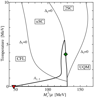
Figure 1: Enclosed with solid thick lines is the unstable region for $A_{1,2}$ on the phase diagram (see Fig. 1 in Ref. Fukushima:2004zq and explanations therein). The critical end-point is marked by a square below which the phase transition from the uSC to the 2SC phase or unpaired quark matter (UQM) is first order. A triangle indicates the gCFL onset located at $M_{s}^{2}/\mu=47.1\;{\rm MeV}$.

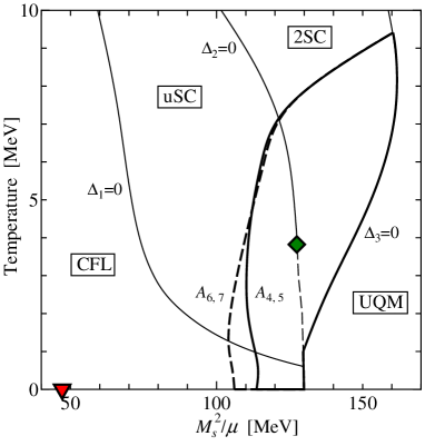
Figure 2: Enclosed with solid and dashed thick lines are the unstable regions for $A_{4,5}$ and $A_{6,7}$ respectively.

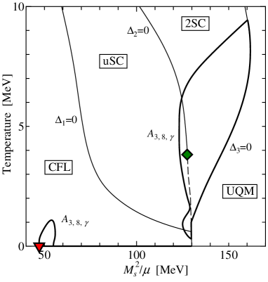
Figure 3: Enclosed with solid thick lines is the unstable region for one or two of eigenmodes consisting of $A_{3}$, $A_{8}$, and $A_{\gamma}$.

The purpose of this paper is to compute the Debye and Meissner masses in the (g)CFL phase and to present detailed analyses on the nature of chromomagnetic instability which occurs in connection with the presence of gapless quarks. Our central results are condensed in the unstable regions on the phase diagram presented in Figs. 1, 2, and 3. In both the CFL and gCFL phases there is no mixing with other gluons for $A_{1}$, $A_{2}$, $A_{4}$, $A_{5}$, $A_{6}$, and $A_{7}$, among which two gluons of $(A_{1},A_{2})$, $(A_{4},A_{5})$, and $(A_{6},A_{7})$ respectively have the same screening masses. We shall write $A_{1,2}$ for instance to mean whichever of $A_{1}$ or $A_{2}$ equivalently from now on. As for $A_{3}$, $A_{8}$, and the electromagnetic field $A_{\gamma}$, on the other hand, mixing between them arises and thus we have to refer to eigenvalues of the $3\times 3$ mass squared matrix to investigate instability. It should be noted that the color indices are labeled according to the conventional Gell-Mann matrices in color space.

Figure 1 shows the unstable region enclosed with thick lines inside which the Meissner mass squared for $A_{1,2}$ is negative. The phase diagram underlaid is what has been revealed in Ref. Fukushima:2004zq for the case of weak coupling yielding $\Delta_{0}=25\;{\rm MeV}$ at $M_{s}=T=0$. The gCFL phase starts appearing at $M_{s}^{2}/\mu=47.1\;{\rm MeV}$ which is well close to the kinematical estimate $(M_{s}^{2}/\mu)_{\rm c}\simeq 2\Delta$. In the vicinity of the phase boundary line on which one of three gaps vanishes, i.e., $\Delta_{2}=0$, there comes out a rather complicated structure which is not robust but strongly depends on a choice of the coupling strength. We will not present results for other coupling cases as done in Ref. Fukushima:2004zq , for our purpose here is not to disclose the phase structure but to argue characteristic features of chromomagnetic instability and to settle where it becomes relevant on the phase diagram.

We observe that instability grows for $A_{1,2}$ as soon as the gCFL state occurs at zero temperature. The instability penetrates from the CFL region where all $u$-$d$, $d$-$s$, and $s$-$u$ quarks make Cooper pairs into the uSC region where $u$-$d$ and $s$-$u$ quarks remain to pair, but never enters the 2SC region where only the $u$-$d$ quark pairing gap is nonvanishing. Actually in the 2SC phase, $A_{1,2}$ become irrelevant to the Higgs-Anderson mechanism, and therefore the Meissner mass for $A_{1,2}$ must be zero there.

The unstable regions for $A_{4,5}$ and $A_{6,7}$ are depicted in Fig. 2. In the 2SC phase there is no discrimination between $A_{4,5}$ and $A_{6,7}$ and the difference is manifested only when quark matter lies in the CFL or uSC phase. Our mapping is consistent with all of the known results both in the 2SC phase Huang:2004bg and in the CFL phase Casalbuoni:2004tb ; no instability takes place near the gCFL onset for $A_{4,5}$ nor $A_{6,7}$, while the large $M_{s}^{2}/\mu$ regions exhibit instability which turns out to be related to the g2SC instability. At small temperatures and large $M_{s}^{2}/\mu$ the Meissner masses squared for $A_{4,5}$ and $A_{6,7}$ are negative until the system reaches the phase boundary from which the system enters the phase of unpaired quark matter (UQM).

It seems to be somewhat tricky to understand the unstable regions for mixed modes of $A_{3}$, $A_{8}$, and $A_{\gamma}$ shown in Fig. 3. At zero or extremely low temperatures whose energy scale is determined by the electron contribution as discussed later, the whole gCFL phase is unstable and our results qualitatively agree with Ref. Casalbuoni:2004tb . At finite temperature there are two distinct regions where instability remains. The instability near the gCFL onset eventually disappears as the temperature grows, while the instability at larger $M_{s}^{2}/\mu$ goes further into the 2SC phase. In fact in the 2SC phase, $A_{3}$ decouples from others and its Meissner mass is reduced to zero, and one of the two eigenmodes composed of $A_{8}$ and $A_{\gamma}$ exhibits chromomagnetic instability as is consistent with the findings in the g2SC phase Huang:2004bg . For even stronger coupling when the 2SC (not necessarily g2SC) phase is possible at zero temperature (see Fig. 17 in Ref. Fukushima:2004zq ), we have numerically checked that instability at larger $M_{s}^{2}/\mu$ starts exactly at the g2SC onset.

The exact correspondence between the gapless and instability onsets is apparent only at zero temperature since the finite-temperature effects allow for thermal quark excitations which are not clearly distinguishable from quarks in the blocking region. An interesting manifestation of this is the unstable region in the uSC phase in which there are no gapless quarks below $T\sim 5\;{\rm MeV}$ (see the dotted curve in the uSC region shown in Fig. 1 in Ref. Fukushima:2004zq ). In a sense, at finite temperature, we can say that the instability penetrates into gapped sides, as is also observed from Fig. 5 in Ref. Alford:2005qw .

We are explaining how we have come by these instability mappings in a numerical way in later discussions, starting with the following subsections in which we shall make a brief review of the gCFL phase and of the derivation of the Debye and Meissner screening masses of gauge fields. The readers who are already familiar with these basics can skip most of them and jump to Sec. II.

I.1 Gapless CFL phase

Our strategy to approach the Debye and Meissner masses is based on the thermodynamic potential that has been formulated within an effective model. In the following subsubsections, we discuss the model and approximations to describe the gCFL phase, and then illustrate the quark excitation energies as a function of the momentum (i.e. the dispersion relations).

I.1.1 Model and approximations

In this paper we adopt essentially the same model and approximations as used in Refs. Alford:2003fq ; Fukushima:2004zq . The only difference is that the $M_{s}$ effect is incorporated as an effective chemical potential shift. This approximation is necessary to relate the Meissner mass to the potential curvature with respect to gluon source fields in a simple way. The model employed here is the Nambu–Jona-Lasinio (NJL) model with four-fermion interaction. In our model study we assume that the predominant diquark condensate is antisymmetric in Dirac indices, antisymmetric in color, and thus antisymmetric in flavor;

$$\langle\psi^{a}_{i}C\gamma_{5}\psi^{b}_{j}\rangle\sim\Delta_{1}\epsilon^{ab1}\epsilon_{ij1}\!+\!\Delta_{2}\epsilon^{ab2}\epsilon_{ij2}\!+\!\Delta_{3}\epsilon^{ab3}\epsilon_{ij3}\,,$$ (1)

where ($i$,$j$) and ($a$,$b$) represent the flavor indices ($u$,$d$,$s$) and the color triplet indices (red,green,blue) respectively. The gap parameters $\Delta_{1}$, $\Delta_{2}$, and $\Delta_{3}$ describe a $9\times 9$ matrix in color-flavor space that takes the form,

$$\boldsymbol{\Delta}=\left(\begin{array}[]{ccccccccc}0&\Delta_{3}&\Delta_{2}&0&0&0&0&0&0\\ \Delta_{3}&0&\Delta_{1}&0&0&0&0&0&0\\ \Delta_{2}&\Delta_{1}&0&0&0&0&0&0&0\\ 0&0&0&0&\makebox[11.99998pt][r]{$-\Delta$}_{3}&0&0&0&0\\ 0&0&0&\makebox[11.99998pt][r]{$-\Delta$}_{3}&0&0&0&0&0\\ 0&0&0&0&0&0&\makebox[11.99998pt][r]{$-\Delta$}_{2}&0&0\\ 0&0&0&0&0&\makebox[11.99998pt][r]{$-\Delta$}_{2}&0&0&0\\ 0&0&0&0&0&0&0&0&\makebox[11.99998pt][r]{$-\Delta$}_{1}\\ 0&0&0&0&0&0&0&\makebox[11.99998pt][r]{$-\Delta$}_{1}&0\\ \end{array}\right)$$ (2)

in the basis $(ru,gd,bs,gu,rd,rs,bu,bd,gs)$. In the same way as in Refs. Alford:2003fq ; Fukushima:2004zq , we ignore diquark condensates which are symmetric in color, though we know that they do not break any new symmetry and consequently can take a finite value. This approximation is motivated by the fact that the QCD interaction is repulsive between quarks in this channel and such diquark condensates have been actually known to be insignificant quantitatively Ruster:2004eg .

In the mean-field approximation where the condensates (1) are relevant, we only have to consider the four-fermion interaction in the diquark-diquark channel that can be generally in hand after appropriate Fierz transformation. That is,

$${\cal L}=\bar{\psi}(i\hbox to5.30904pt{\hbox to0.0pt{\hbox to5.30904pt{\hss/\hss}\hss}\hbox{$\partial$}}+\boldsymbol{\mu}\gamma^{0}-\boldsymbol{M})\psi+{\cal L}_{\text{int}}\,,$$ (3)

where

$$\begin{split}{\cal L}_{\text{int}}&=\frac{G}{4}(\bar{\psi}^{a}_{i}i\gamma_{5}\epsilon^{ab\eta}\epsilon_{ij\eta}C\bar{\psi}^{Tb}_{j})\\ &\qquad\qquad\times(\psi^{Ta^{\prime}}_{i^{\prime}}Ci\gamma_{5}\epsilon^{a^{\prime}b^{\prime}\eta}\epsilon_{i^{\prime}j^{\prime}\eta}\psi^{b^{\prime}}_{j^{\prime}})\,.\end{split}$$ (4)

Here the mass matrix $\boldsymbol{M}$ is unity in color and $\text{diag}(0,0,M_{s})$ in flavor ($u$,$d$,$s$) space in our approximation and $\boldsymbol{\mu}$ the matrix of quark chemical potentials in color-flavor space. Bold symbols generally denote matrices in color-flavor space. The charge conjugation matrix is $C=i\gamma^{2}\gamma^{0}$.

The effect of nonzero $\boldsymbol{M}$ on the particle dispersion relation becomes apparent in the vicinity of the Fermi surface, where it can be well approximated by a shift in quark chemical potentials by $\boldsymbol{MM}^{\dagger}/2\mu$. We shall make use of this prescription that actually turns out to be essential to allow us to relate the Meissner mass to the potential curvature. In the present work, as in Refs. Alford:2003fq ; Fukushima:2004zq , $\boldsymbol{M}$ is not current but constituent quark mass and is treated as an input parameter. We know that this approximation provides a correct phase structure unless the chiral phase transition cuts deeply into the gCFL region under the choice of strong coupling in the chiral sector Abuki:2004zk .

Chemical potentials are fixed by equilibration and neutrality. Stable quark matter should be a color singlet as a whole and neutral in the electric charge under $\beta$-equilibrium. Color singletness is a more stringent condition than neutrality. It has been shown, however, that no energy cost is needed to project a neutral state onto a singlet state in color in the thermodynamic limit Amore:2001uf . Hence, it is sufficient to impose global neutrality with respect to the electric and color charges. To describe that, we shall consider $\mu_{e}$, $\mu_{3}$, and $\mu_{8}$ that are coupled to negative $Q=\text{diag}({\textstyle\frac{2}{3}},-{\textstyle\frac{1}{3}},-{\textstyle\frac{1}{3}})$ in flavor ($u$,$d$,$s$) space so that a positive $\mu_{e}$ corresponds to the electron density, $T_{3}=\text{diag}({\textstyle\frac{1}{2}},-{\textstyle\frac{1}{2}},0)$, and ${\textstyle\frac{2}{\sqrt{3}}}T_{8}=\text{diag}({\textstyle\frac{1}{3}},{\textstyle\frac{1}{3}},-{\textstyle\frac{2}{3}})$ in color (red, green, blue) space, respectively. Then, 9 diagonal components of the effective chemical potential matrix $\boldsymbol{\mu}_{\text{eff}}$ (including the shift by $\boldsymbol{MM}^{\dagger}/2\mu$) in color-flavor space are explicitly

$$\begin{array}[]{rcl}\mu_{ru}&=&\mu-{\textstyle\frac{2}{3}}\mu_{e}+{\textstyle\frac{1}{2}}\mu_{3}+{\textstyle\frac{1}{3}}\mu_{8},\\[4.30554pt] \mu_{gd}&=&\mu+{\textstyle\frac{1}{3}}\mu_{e}-{\textstyle\frac{1}{2}}\mu_{3}+{\textstyle\frac{1}{3}}\mu_{8},\\[4.30554pt] \mu_{bs}&=&\mu+{\textstyle\frac{1}{3}}\mu_{e}-{\textstyle\frac{2}{3}}\mu_{8}-{\textstyle\frac{M_{s}^{2}}{2\mu}},\\[12.91663pt] \mu_{gu}&=&\mu-{\textstyle\frac{2}{3}}\mu_{e}-{\textstyle\frac{1}{2}}\mu_{3}+{\textstyle\frac{1}{3}}\mu_{8},\\[4.30554pt] \mu_{rd}&=&\mu+{\textstyle\frac{1}{3}}\mu_{e}+{\textstyle\frac{1}{2}}\mu_{3}+{\textstyle\frac{1}{3}}\mu_{8},\\[12.91663pt] \mu_{rs}&=&\mu+{\textstyle\frac{1}{3}}\mu_{e}+{\textstyle\frac{1}{2}}\mu_{3}+{\textstyle\frac{1}{3}}\mu_{8}-{\textstyle\frac{M_{s}^{2}}{2\mu}},\\[4.30554pt] \mu_{bu}&=&\mu-{\textstyle\frac{2}{3}}\mu_{e}-{\textstyle\frac{2}{3}}\mu_{8},\\[12.91663pt] \mu_{bd}&=&\mu+{\textstyle\frac{1}{3}}\mu_{e}-{\textstyle\frac{2}{3}}\mu_{8}\ .\\[4.30554pt] \mu_{gs}&=&\mu+{\textstyle\frac{1}{3}}\mu_{e}-{\textstyle\frac{1}{2}}\mu_{3}+{\textstyle\frac{1}{3}}\mu_{8}-{\textstyle\frac{M_{s}^{2}}{2\mu}},\\[4.30554pt] \end{array}$$ (5)

The gap parameters corresponding to (1) in this model are precisely defined as

$$\Delta_{\eta}={\textstyle\frac{1}{2}}G\langle\psi^{T\alpha}_{i}Ci\gamma_{5}\epsilon^{\alpha\beta\eta}\epsilon_{ij\eta}\psi^{\beta}_{j}\rangle.$$ (6)

With all these definitions, if we choose Nambu-Gor’kov basis as $\Psi(p)=(\psi(p),C\bar{\psi}^{T}(-p))^{T}$, we can express the mean-field (inverse) quark propagator in a simple form,

$$iS^{-1}(p)=\left(\begin{array}[]{cc}\hbox to5.03125pt{\hbox to0.0pt{\hbox to5.03125pt{\hss/\hss}\hss}\hbox{$p$}}+\boldsymbol{\mu}\gamma^{0}&i\gamma_{5}\boldsymbol{\Delta}\\ i\gamma_{5}\boldsymbol{\Delta}&\hbox to5.03125pt{\hbox to0.0pt{\hbox to5.03125pt{\hss/\hss}\hss}\hbox{$p$}}-\boldsymbol{\mu}\gamma^{0}\end{array}\right)$$ (7)

after rearranging the Dirac matrices. The quark propagator is a $72\times 72$ matrix in color, flavor, spin, and Nambu-Gor’kov space. From zeros of the inverse propagator, we can read 72 energy dispersion relations $\varepsilon_{i}(p)$. The thermodynamic potential $\Omega$ is thus written in terms of $\varepsilon_{i}$’s as

$$\begin{split}\Omega&=-\frac{1}{8\pi^{2}}\int_{0}^{\Lambda}\!\!dp\,p^{2}\sum_{j=1}^{72}\Bigl{\{}|\varepsilon_{i}|+2T\ln\bigl{(}1+e^{-|\varepsilon_{i}|/T}\bigr{)}\Bigr{\}}\\ &+\frac{1}{G}\bigl{(}\Delta_{1}^{2}+\Delta_{2}^{2}+\Delta_{3}^{2}\bigr{)}-\frac{\mu_{e}^{4}}{12\pi^{2}}-\frac{\mu_{e}^{2}T^{2}}{6}-\frac{7\pi^{2}T^{4}}{180}\end{split}$$ (8)

with the electron contribution in the last three terms. In order to fix three gap parameters and three chemical potentials at each $M_{s}$, $\mu$, and $T$, we will simultaneously solve three gap equations,

$$\frac{\partial\Omega}{\partial\Delta_{1}}=\frac{\partial\Omega}{\partial\Delta_{2}}=\frac{\partial\Omega}{\partial\Delta_{3}}=0\,,$$ (9)

and three neutrality conditions,

$$\frac{\partial\Omega}{\partial\mu_{e}}=\frac{\partial\Omega}{\partial\mu_{3}}=\frac{\partial\Omega}{\partial\mu_{8}}=0\,.$$ (10)

Here $\Lambda$ in (8) is the ultraviolet cut-off parameter and we use $\Lambda=800\;{\rm MeV}$ as in Refs. Alford:2003fq ; Fukushima:2004zq . The coupling constant $G$ is chosen to yield $\Delta_{0}=25\;{\rm MeV}$ when both $M_{s}$ and $T$ are zero. In the present work we take the quark chemical potential $\mu=500\;{\rm MeV}$ that roughly corresponds to 10 times the normal nuclear density in the model.

When $M_{s}$ is not so large as to disrupt any Cooper pair, $\mu_{e}$, $\mu_{3}$, and $\mu_{8}$ satisfying electric and color neutrality have been analyzed at zero temperature in a model-independent way Alford:2002kj . Two of three can be fixed as a function of the third that we will choose $\mu_{e}$ here, then

$$\mu_{3} =\mu_{e},$$ (11)

$$\mu_{8} =-\frac{M_{s}^{2}}{2\mu}+\frac{\mu_{e}}{2}.$$ (12)

The important feature of the CFL phase we should note is that the thermodynamic potential (8) at $T=0$ with the electron contribution disregarded is independent of

$$\mu_{{\tilde{Q}}}=-{\textstyle\frac{4}{9}}\bigl{(}\mu_{e}+\mu_{3}+{\textstyle\frac{1}{2}}\mu_{8}\bigr{)},$$ (13)

that is the chemical potential for ${\tilde{Q}}=Q-T_{3}-\frac{1}{\sqrt{3}}T_{8}$. It is known that ${\tilde{Q}}$ is a generator of the “rotated electromagnetism” that is never broken by any condensate of the form (1). At zero temperature ${\tilde{Q}}$-charged excitations in CFL quark matter are all gapped and the CFL phase is a ${\tilde{Q}}$-insulator Rajagopal:2000ff .

In the presence of the electron contribution to the thermodynamic potential, in reality, there is a gentle curvature on the plateau of the thermodynamic potential provided by the last three terms in (8) which select $\mu_{e}=0$, meaning zero electron density. Although it makes only slight changes in energy, the existence of the electron effects is crucial in understanding the $A_{1,2}$ instability.

I.1.2 Gapless dispersion relations

Since the gap matrix (2) is block-diagonal, the $72\times 72$ quark propagator matrix is block-diagonal as well in color-flavor space and can be divided into four parts; one $24\times 24$ part for $ru$-$gd$-$bs$ quark pairing with $\Delta_{1}$, $\Delta_{2}$, and $\Delta_{3}$ and three $16\times 16$ parts for quark pairing of $bd$-$gs$ with $\Delta_{1}$, $rs$-$bu$ with $\Delta_{2}$, and $gu$-$rd$ with $\Delta_{3}$. It might be possible but quite hard to handle the $24\times 24$ part analytically. Fortunately, as we will see shortly, this $24\times 24$ intricate part has little to do with chromomagnetic instability, so we will limit our discussion here to the propagator for $bd$-$gs$, $rs$-$bu$, and $gu$-$rd$ pairings.

Leaving the explicit expression of the quark propagator until Sec. II, let us elucidate here the quark energy dispersion relations obtained from zeros of the inverse propagator. In general for the $16\times 16$ part involving two species $A$ and $B$ quarks the energy dispersion relation takes the form,

$$\varepsilon_{\text{$A$-$B$}} =\sqrt{(p-\bar{\mu}_{\text{$A$-$B$}})^{2}+\Delta_{AB}^{2}}+\delta\mu_{\text{$A$-$B$}},$$ (14)

$$\tilde{\varepsilon}_{\text{$A$-$B$}} =\sqrt{(p+\bar{\mu}_{\text{$A$-$B$}})^{2}+\Delta_{AB}^{2}}+\delta\mu_{\text{$A$-$B$}}$$ (15)

for quasi-particle and antiparticle excitations respectively, where $\bar{\mu}_{\text{$A$-$B$}}={\textstyle\frac{1}{2}}(\mu_{A}+\mu_{B})$ and $\delta\mu_{\text{$A$-$B$}}={\textstyle\frac{1}{2}}(\mu_{A}-\mu_{B})$ and $\Delta_{AB}$ is the energy gap for $A$-$B$ pairing. In our definition $\delta\mu_{\text{$A$-$B$}}=-\delta\mu_{\text{$B$-$A$}}$. Gapless dispersion relations come about once

$$|\delta\mu_{\text{$A$-$B$}}|>\Delta_{AB}.$$ (16)

Then, using effective chemical potentials (5) with the known CFL solutions (11) and (12), we have

$$\delta\mu_{\text{$gu$-$rd$}} =-{\textstyle\frac{1}{2}}\mu_{e}-{\textstyle\frac{1}{2}}\mu_{3}=-\mu_{e}\,,$$ (17)

$$\delta\mu_{\text{$rs$-$bu$}} ={\textstyle\frac{1}{2}}\mu_{e}+{\textstyle\frac{1}{4}}\mu_{3}+{\textstyle\frac{1}{2}}\mu_{8}-{\textstyle\frac{M_{s}^{2}}{4\mu}}=\mu_{e}-{\textstyle\frac{M_{s}^{2}}{2\mu}}\,,$$ (18)

$$\delta\mu_{\text{$bd$-$gs$}} ={\textstyle\frac{1}{4}}\mu_{3}-{\textstyle\frac{1}{2}}\mu_{8}+{\textstyle\frac{M_{s}^{2}}{4\mu}}={\textstyle\frac{M_{s}^{2}}{2\mu}}\,,$$ (19)

and

$$\bar{\mu}_{\text{$gu$-$rd$}}=\bar{\mu}_{\text{$bd$-$gs$}}=\bar{\mu}_{\text{$rs$-$bu$}}=\mu-{\textstyle\frac{M_{s}^{2}}{6\mu}}$$ (20)

in the CFL phase. If it were not for the electron terms in the thermodynamic potential, $\mu_{e}$ could lie anywhere as far as it does not disrupt the pairing of $gu$-$rd$ nor $rs$-$bu$ quarks which are ${\tilde{Q}}$-charged. In the region between the dashed and dot-dashed curves shown in Fig. 4, the system remains to be a ${\tilde{Q}}$-insulator, meaning the bandgap. The CFL solution ceases to exist at the point where these two curves meet, before which a first-order phase transition to unpaired quark matter takes place as indicated by the dotted vertical line (see discussions in Ref. Alford:2003fq for details).

Figure 4: Boundaries for the gapless conditions (16) for $bd$-$gs$ (solid), $rs$-$bu$ (dashed), and $gu$-$rd$ (dot-dashed) quarks. Because $bd$-$gs$ quarks are neutral in ${\tilde{Q}}$-charge, the system can go through the solid line, though the bandgap is edged with the dashed and dot-dashed lines and quark matter is a ${\tilde{Q}}$-insulator between these two boundaries. With the inclusion of the electron contributions to the thermodynamic potential, $\mu_{e}$ is zero until $M_{s}^{2}/\mu$ reaches the $bd$-$gs$ line, and then $\mu_{e}$ goes up slightly below the $rs$-$bu$ dashed boundary. This is because the ${\tilde{Q}}$-charged electrons must be canceled by a small disruption of $rs$-$bu$ quark pairing.

By substituting $\mu_{e}=0$, as is favored in the CFL phase with electrons, for the above expressions, we readily realize that the $bd$-$gs$ and $rs$-$bu$ dispersion relations are identical supposing $\Delta_{1}=\Delta_{2}=\Delta$. In fact, the $bd$-$gs$ and $rs$-$bu$ quark pairings are breached at the same time when

$$|\delta\mu_{\text{$bd$-$gs$}}|=|\delta\mu_{\text{$rs$-$bu$}}|=\frac{M_{s}^{2}}{2\mu}>\Delta\,,$$ (21)

which corresponds to the fact that in Fig. 4 the solid and dashed lines cross at $\mu_{e}=0$. This coincidence of the gapless onset locations for $bd$-$gs$ and $rs$-$bu$ quarks is responsible for instability for $A_{1,2}$ in the gCFL phase, as only $A_{1,2}$ can excite a pair of $rs$ and $gs$ quarks at once (see Fig. 6). In other words, if the electron terms are absent and $\mu_{e}$ is chosen to be positive, say $\sim 10\;{\rm MeV}$, the $A_{1,2}$ instability would disappear, while there would remain the instability for other gluons.

Figure 5: Energy dispersion relations for $bd$-$gs$ (solid) and $rs$-$bu$ (dashed) quarks at $M_{s}^{2}/\mu=80\;{\rm MeV}$. The dotted curve is one that has the lowest energy among the 24 $ru$-$gd$-$bs$ dispersion relations.

Once quark matter enters the gCFL phase with larger $M_{s}^{2}/\mu$ than the onset, the $bd$-$gs$ and $rs$-$bu$ quark dispersion relations are both gapless but no longer degenerated. The blocking momentum region for $bd$-$gs$ quarks becomes wider with increasing $M_{s}^{2}/\mu$ as shown by the solid curve in Fig. 5 and $\Delta_{1}$ decreases accordingly because quarks within the blocking region cannot participate in pairing. Since $rs$ and $bu$ quarks have nonzero ${\tilde{Q}}$-charge, the blocking momentum region for $rs$-$bu$ quarks is not allowed to be arbitrarily wider and is determined by the requirement to cancel ${\tilde{Q}}$-charge brought by electrons whose density is $\sim\mu_{e}^{3}$. That means, the width of the blocking momentum region for $rs$-$bu$ quarks is estimated as $\delta p\sim\mu_{e}^{3}/3\bar{\mu}^{2}\ll\bar{\mu}$ Alford:2003fq . The actual form of the $rs$-$bu$ dispersion relation is, as a result, kept to be almost quadratic with a tiny blocking region anywhere in the gCFL phase as seen by the dashed curve in Fig. 5.

Although the $ru$-$gd$-$bs$ part is hard to anticipate a priori, there is no gapless mode involved in this sector. The dotted curve in Fig. 5 represents one of energy dispersion relations for $ru$-$gd$-$bs$ quarks that has the lowest energy among them. It is clear from the figure that $ru$-$gd$-$bs$ quarks are all gapped at $M_{s}^{2}/\mu=80\;{\rm MeV}$ and it is also the case for larger $M_{s}^{2}/\mu$. Hence, the three (solid, dashed, and dot-dashed) lines drawn for $bd$-$gs$, $rs$-$bu$, and $gu$-$rd$ quarks respectively in Fig. 4 suffice for judging if gapless quarks are present or not.

I.2 Debye and Meissner screening masses

In a medium at finite temperature and density the gauge fields are screened by the polarization of charged thermal excitations. The screening effect on the gauge fields differs depending on the longitudinal and transverse directions due to the lack of Lorentz invariance. The screening mass, which is the inverse of the screening length, in the longitudinal direction is called the (chromo)electric or Debye screening mass, and in (color) superconductors in particular the transverse screening mass, the (chromo)magnetic or Meissner screening mass in QED (QCD). In the normal phase any perturbative calculation leads to vanishing magnetic mass in the static limit. In the superconducting phase, on the other hand, a finite magnetic screening mass results from the Higgs-Anderson mechanism and embodies the Meissner effect so that superconductors can exclude the magnetic field.

The Debye and Meissner masses are calculated from the eigenvalues of the mass squared matrix in color defined by the self-energies;

$$m_{D,\alpha\beta}^{2} =-\lim_{q\to 0}\Pi_{\alpha\beta}^{00}(\omega=0,\vec{q}),$$ (22)

$$m_{M,\alpha\beta}^{2} ={\textstyle\frac{1}{2}}\lim_{q\to 0}\bigl{(}\delta_{ij}-\widehat{q}_{i}\widehat{q}_{j}\bigr{)}\Pi_{\alpha\beta}^{ij}(\omega=0,\vec{q}),$$ (23)

where ($\alpha$,$\beta$) represent the color octet (or photon) indices and we defined $\widehat{q}=\vec{q}/|\vec{q}|$, and $\Pi_{\alpha\beta}^{\mu\nu}$ is the self-energy with the Lorentz indices ($\mu$,$\nu$) for the gluons ($\alpha,\beta\leq 8$) or photon ($\gamma$ instead of $\alpha,\beta$) or their mixing. (We always use the subscript $\gamma$ for the sake of meaning photon.) At the one-loop level at high density, the quark loop contribution to $\Pi_{\alpha\beta}^{\mu\nu}$, which is proportional to $\mu^{2}$, is predominant, so we shall consider only the polarization tensor coming from one-loop diagrams of quarks.

In the symmetric CFL state with $M_{s}=0$, the mass squared matrix is diagonal in color and all eight gluons have the same screening mass. The Debye and Meissner masses in a color superconductor have been calculated diagrammatically in Ref. Rischke:2000qz and we shall quote the results here;

$$m_{D}^{2} =\frac{21-8\ln 2}{6}m_{g}^{2}\simeq 2.576m_{g}^{2}\,,$$ (24)

$$m_{M}^{2} =\frac{1}{3}m_{D}^{2}\simeq 0.859m_{g}^{2}$$ (25)

for all eight gluons. Here $m_{g}^{2}=g^{2}\mu^{2}/6\pi^{2}$ and $g$ is the strong coupling constant. Note that our definition of $m_{g}^{2}$ is different by a factor $N_{f}=3$ from the definition given in Ref. Rischke:2000qz .

Once mixing between gluons and photon, which exists among $A_{8}$ and $A_{\gamma}$ in the CFL phase at $M_{s}=0$, and generally among $A_{3}$, $A_{8}$, and $A_{\gamma}$ for $M_{s}\neq 0$, is taken into account, the screening masses are to be modified. They actually have been evaluated analytically only when $M_{s}=0$ Schmitt:2003aa and after diagonalization two eigenvalues composed of $A_{8}$ and $A_{\gamma}$ read

$$\tilde{m}_{D,88}^{2} =\Bigl{(}1+\frac{4}{3}\frac{e^{2}}{g^{2}}\Bigr{)}m_{D}^{2}\,,$$ (26)

$$\tilde{m}_{M,88}^{2} =\Bigl{(}1+\frac{4}{3}\frac{e^{2}}{g^{2}}\Bigr{)}m_{M}^{2}\,,$$ (27)

$$\tilde{m}_{D,\gamma\gamma}^{2} =\tilde{m}_{M,\gamma\gamma}^{2}=0\,,$$ (28)

where $e$ is the electromagnetic coupling constant. The last relation (28) follows from the facts that the condensates (1) leave a ${\rm U}(1)_{\tilde{Q}}$ symmetry unbroken (that is; $\tilde{m}_{M,\gamma\gamma}^{2}=0$), and that the system is a ${\tilde{Q}}$-insulator in which ${\tilde{Q}}$-charged excitations are all gapped (that is; $\tilde{m}_{D,\gamma\gamma}^{2}=0$).

For later convenience we shall carefully look into how these analytical expressions (24) and (25) are structured from distinct contributions of particles and antiparticles. When quarks are massless, the quark propagator can be specifically separated into the particle and antiparticle parts (see Eq. (40)). At the quark one-loop level, the gluon or photon self-energies consist of the particle-particle, particle-antiparticle, and antiparticle-antiparticle excitations. (In the case of the normal phase the particle-particle excitations in the vector channels would be to be articulated as the particle-hole excitations.) The last contribution from only the antiparticle excitations is just negligible so that we shall always omit it in our discussion.

In the $2\times 2$ space of Nambu-Gor’kov doubling, the quark propagator has not only the diagonal (normal) components but also the off-diagonal (abnormal) components proportional to the gap $\Delta$ that connect two quasi-particles.

The Debye mass arises only from the particle-particle contribution. It can be further divided into the Nambu-Gor’kov diagonal and off-diagonal parts as follows;

$$m_{D}^{2}=[m_{D}^{2}]_{\text{diag}}+[m_{D}^{2}]_{\text{off}}\,,$$ (29)

where

$$[m_{D}^{2}]_{\text{diag}}=\frac{9}{2}m_{g}^{2}\,,$$ (30)

$$[m_{D}^{2}]_{\text{off}}=-\biggl{(}1+\frac{4}{3}\ln 2\biggr{)}m_{g}^{2}\,.$$ (31)

The sum of these two parts properly reproduces (24) as it should.

In evaluating the Meissner mass, on the other hand, it is essentially important to note that the particle-antiparticle excitation produces a significant contribution comparable to the particle-particle one. The Meissner mass consists of the diagonal and off-diagonal parts,

$$m_{M}^{2}=[m_{M}^{2}]_{\text{diag}}+[m_{M}^{2}]_{\text{off}}\,,$$ (32)

that is further split into the particle-particle (p-p) and particle-antiparticle (p-a) parts,

$$[m_{M}^{2}]_{\text{diag}}=[m_{M}^{2}]_{\text{diag(p-p)}}+2[m_{M}^{2}]_{\text{diag(p-a)}}$$ (33)

with

$$[m_{M}^{2}]_{\text{diag(p-p)}} =-\frac{1}{3}[m_{D}^{2}]_{\text{diag}}\,,$$ (34)

$$[m_{M}^{2}]_{\text{diag(p-a)}} =\frac{3}{2}m_{g}^{2}\,,$$ (35)

and

$$[m_{M}^{2}]_{\text{off}}=[m_{M}^{2}]_{\text{off(p-p)}}=\frac{1}{3}[m_{D}^{2}]_{\text{off}}\,,$$ (36)

from which we can easily make sure $m_{M}^{2}={\textstyle\frac{1}{3}}m_{D}^{2}$ as is well-known in the CFL phase Rischke:2000qz ; Son:1999cm . The particle-antiparticle contribution in the off-diagonal part $[m_{M}^{2}]_{\text{off(p-a)}}$ is vanishingly small, so we dropped it off from the above relations.

It is of great importance to realize that the diagonal p-p contribution to the Meissner mass is negative one third of the Debye mass counterpart, while the p-a excitations provide a positive contribution that is twice larger than the p-p’s. Adding them together we finally acquire the Meissner mass contribution that is positive one third of the Debye mass contribution. In the off-diagonal part, in contrast, the situation is much simpler and the ratio is positive one third itself.

In other words, in the diagonal part, the p-p loops always tend to induce paramagnetism, while diamagnetism originates from the p-a loops. Usually in the superconducting phase, the diamagnetic tendency is greater enough to bring about the Meissner effect. In gapless superconductors, however, antiparticles are never gapless and only the p-p loops are abnormally enhanced due to gapless quarks and their large density of states near the Fermi surface causes the opposite phenomenon to the Meissner effect, i.e., chromomagnetic instability. Also, this can be seen from the relations (34) and (36) which hold in the presence of finite $M_{s}$ or even in the gCFL phase. In the gCFL phase, a large density of states leads to a large Debye mass. Then, through (34) and (36), it should be accompanied by a large negative contribution to the Meissner mass squared, which eventually results in chromomagnetic instability.

As for (35), because the $M_{s}$ dependence of antiparticle excitations is suppressed by $M_{s}/\mu$, the relation is hardly changed for any $M_{s}\ll\mu$.

II computation of self-energies

In this section we shall diagrammatically compute the calculable parts of one-loop self-energies for gluons and photon and derive the analytical expression for the singular part of the Debye and Meissner masses.

Using the mean-field quark propagator $S(p)$, and the vertex matrices, $\Gamma^{\mu}_{\alpha}$, in color, flavor, spin, and Nambu-Gor’kov space, we can write the one-loop self-energies in a general form as

$$-i\Pi_{\alpha\beta}^{\mu\nu}(q)=-\frac{1}{2}\int^{T}\!\!\!\frac{d^{4}p}{(2\pi)^{4}}\,\text{tr}\,\Gamma^{\mu}_{\alpha}S(q+p)\Gamma^{\nu}_{\beta}S(p)\,.$$ (37)

The vertices $\Gamma^{\mu}_{\alpha}$ take a matrix form,

$$\Gamma^{\mu}_{\alpha}=\left[\begin{array}[]{cc}-ig\gamma^{\mu}T_{\alpha}\delta_{ij}&0\\ 0&ig\gamma^{\mu}T_{\alpha}\delta_{ij}\end{array}\right]$$ (38)

for gluons ($\alpha=1,\dots,8$) where $T_{\alpha}$ are the ${\rm SU}(3)_{\text{color}}$ generators defined by the Gell-Mann matrices in color space and normalized as $\text{tr}T_{\alpha}T_{\beta}={\textstyle\frac{1}{2}}\delta_{\alpha\beta}$. For photon the vertex reads

$$\Gamma^{\mu}_{\gamma}=\left[\begin{array}[]{cc}-ie\gamma^{\mu}Q_{ij}&0\\ 0&ie\gamma^{\mu}Q_{ij}\end{array}\right],$$ (39)

which is unity in color. We see that the flavor is not changed at any vertices but the color can be converted through the off-diagonal components in $T_{1}$, $T_{2}$, $T_{4}$, $T_{5}$, $T_{6}$, and $T_{7}$. We call the gluons corresponding to $T_{3}$ and $T_{8}$ as the color-diagonal gluons.

The quark propagator is divided into the particle and antiparticle parts by the energy projection operators $\Lambda_{p}^{\pm}={\textstyle\frac{1}{2}}(1\pm\gamma^{0}\vec{\gamma}\cdot\widehat{p})$. The explicit propagator in the $bd$-$gs$ sector, for instance, can be written down after some rearrangement of the Nambu-Gor’kov (1,2) (where 2 is assigned to the Nambu-Gor’kov doubler in our convention) and color-flavor ($bd$,$gs$) indices, that is, in the basis ($bd$-1,$gs$-2,$gs$-1,$bd$-2), we have

$$\begin{split}&-iS(p)=\left[\begin{array}[]{cccc}\Lambda^{-}_{p}&0&0&0\\ 0&\Lambda^{+}_{p}&0&0\\ 0&0&\Lambda^{-}_{p}&0\\ 0&0&0&\Lambda^{+}_{p}\end{array}\right]\gamma^{0}\left[\begin{array}[]{cc}S^{\rm a}_{\text{$bd$-$gs$}}(p)&0\\ 0&S^{\rm a}_{\text{$gs$-$bd$}}(p)\end{array}\right]\\ &\qquad+\left[\begin{array}[]{cccc}\Lambda^{+}_{p}&0&0&0\\ 0&\Lambda^{-}_{p}&0&0\\ 0&0&\Lambda^{+}_{p}&0\\ 0&0&0&\Lambda^{-}_{p}\end{array}\right]\gamma^{0}\left[\begin{array}[]{cc}S^{\rm p}_{\text{$bd$-$gs$}}(p)&0\\ 0&S^{\rm p}_{\text{$gs$-$bd$}}(p)\end{array}\right]\,,\end{split}$$ (40)

where the antiparticle part is

$$\begin{split}S^{\rm a}_{\text{$A$-$B$}}(p)&=\frac{1}{\bigl{(}p_{0}+\tilde{\varepsilon}_{\text{$A$-$B$}}\bigr{)}\bigl{(}p_{0}-\tilde{\varepsilon}_{\text{$B$-$A$}}\bigr{)}}\\ &\qquad\times\left[\begin{array}[]{cc}p_{0}-(p+\mu_{B})&-i\Delta_{1}\gamma_{5}\gamma^{0}\\ -i\Delta_{1}\gamma_{5}\gamma^{0}&p_{0}+(p+\mu_{A})\end{array}\right]\,,\end{split}$$ (41)

and the particle part is

$$\begin{split}S^{\rm p}_{\text{$A$-$B$}}(p)&=\frac{1}{\bigl{(}p_{0}+\varepsilon_{\text{$A$-$B$}}\bigr{)}\bigl{(}p_{0}-\varepsilon_{\text{$B$-$A$}}\bigr{)}}\\ &\qquad\times\left[\begin{array}[]{cc}p_{0}+(p-\mu_{B})&-i\Delta_{1}\gamma_{5}\gamma^{0}\\ -i\Delta_{1}\gamma_{5}\gamma^{0}&p_{0}-(p-\mu_{A})\end{array}\right]\,.\end{split}$$ (42)

In this representation the structure of the Dirac indices becomes much simpler and is given by $\Lambda^{\pm}_{p}\gamma^{0}$ and $\gamma_{5}\gamma^{0}$ attached with $\Delta$. Then, it is important to notice that the $(\mu,\nu)$ dependence in the integrand of (37) comes from the trace over the Dirac indices alone, that is

$${\cal T}_{\text{diag(p-p)}}^{\mu\nu}(p;q) =\text{tr}\bigl{[}\gamma^{\mu}\Lambda_{q+p}^{+}\gamma^{0}\gamma^{\nu}\Lambda_{p}^{+}\gamma^{0}\bigr{]},$$ (43)

$${\cal T}_{\text{diag(p-a)}}^{\mu\nu}(p;q) =\text{tr}\bigl{[}\gamma^{\mu}\Lambda_{q+p}^{+}\gamma^{0}\gamma^{\nu}\Lambda_{p}^{-}\gamma^{0}\bigr{]}$$ (44)

for p-p and p-a loops made of the Nambu-Gor’kov diagonal components of the propagator (41) and (42). For the Nambu-Gor’kov off-diagonal components we have likewise;

$${\cal T}_{\text{off(p-p)}}^{\mu\nu}(p;q) =\text{tr}\bigl{[}\gamma^{\mu}\Lambda_{q+p}^{+}\gamma_{5}\gamma^{\nu}\Lambda_{p}^{-}\gamma_{5}\bigl{]},$$ (45)

$${\cal T}_{\text{off(p-a)}}^{\mu\nu}(p;q) =\text{tr}\bigl{[}\gamma^{\mu}\Lambda_{q+p}^{+}\gamma_{5}\gamma^{\nu}\Lambda_{p}^{+}\gamma_{5}\bigl{]}\,.$$ (46)

II.1 Singularities in $A_{1,2}$

We will first discuss $A_{1}$ and $A_{2}$ that are degenerated. The generators in color, $T_{1}$ and $T_{2}$, have a non-vanishing component only between red and green and the flavor is kept unchanged at the vertices, so that the self-energy for $A_{1,2}$ stems from four diagrams;

$$\begin{split}\Pi_{11}^{\mu\nu}&=\Pi^{\mu\nu}_{\text{diag($rg;s$)}}+\Pi^{\mu\nu}_{\text{diag($rg;u$)}}\\ &\qquad\quad+\Pi^{\mu\nu}_{\text{diag($rg;d$)}}+\Pi^{\mu\nu}_{\text{off($ru$-$gd$;$gu$-$rd$)}}.\end{split}$$ (47)

Here, diag($rg;s$) means the quark loop composed of the diagonal component of $rs$ and $gs$ quarks (see Fig. 6) and diag($rg;u$) and diag($rg;d$) should be understood in the same manner. The last contribution, off($ru$-$gd$;$gu$-$rd$), represents the self-energy contribution from the off-diagonal components of $ru$-$gd$ and $gu$-$rd$ propagation, that is, the loop made up with $ru$ quarks turning into $gd$ and $rd$ quarks turning into $gu$ as shown in Fig. 7.

Figure 6: An example of diagrams consisting of the diagonal components contributing to the self-energy for $A_{1,2}$.

Figure 7: An example of diagrams consisting of the off-diagonal components contributing to the self-energy for $A_{1,2}$. Neither $ru$-$gd$ nor $gu$-$rd$ propagation involves gapless quarks, so that this diagram could not lead to any singular behavior in the gCFL phase.

In the case of $A_{1}$ (and $A_{2}$ equivalently) only $\Pi^{\mu\nu}_{\text{diag($rg;s$)}}$ may contain gapless quarks in the gCFL phase in both lines of the loop diagram, and is expected to provide a singular contribution. As a matter of fact, the singular part presumably dominates over the screening mass behavior near the gapless onset as a function of $M_{s}$. This expectation is confirmed by the comparison between functional forms of only the $rs$-$gs$ polarization and the full result derived from the potential curvature we are dealing with in the next section. From Fig. 8, taking in the full results in advance, we can clearly observe that the physics near the gCFL onset is to be described by the $rs$-$gs$ excitation only.

Figure 8: Comparison between the $rs$-$gs$ contribution with an offset $0.39$ and the full result for the Meissner mass squared for $A_{1,2}$. This means that the gross feature near the gCFL onset is provided by the $rs$-$gs$ diagram alone.

The Debye screening mass, or $\Pi^{00}$, has only the particle-particle part (and the antiparticle-antiparticle part that is negligible) because ${\cal T}_{\text{diag(p-a)}}^{00}(p;0)={\cal T}_{\text{off(p-a)}}^{00}(p;0)=0$ and is written as

$$\begin{split}&\Pi^{00}_{\text{diag($rg;s$)}}(q\to 0)\\ &=-\frac{g^{2}}{8\pi^{2}}\int dp\,p^{2}\,{\cal T}_{\text{diag(p-p)}}^{00}(p;0)\,{\cal U}_{\text{diag($rg;s$)}}(p)\,,\end{split}$$ (48)

where ${\cal T}_{\text{diag(p-h)}}^{00}(p;0)=2$ and we defined

$$\begin{split}&{\cal U}_{\text{diag($rg;s$)}}=f_{\text{p-p}}[\varepsilon_{\text{$bu$-$rs$}};bd,gs,bu]\\ &+f_{\text{p-p}}[-\varepsilon_{\text{$rs$-$bu$}};bd,gs,bu]+f_{\text{p-p}}[\varepsilon_{\text{$bd$-$gs$}};bu,rs,bd]\\ &+f_{\text{p-p}}[-\varepsilon_{\text{$gs$-$bd$}};bu,rs,bd].\end{split}$$ (49)

The p-p integrand $f_{\text{p-p}}$ is explicitly given by

$$\begin{split}&f_{\text{p-p}}[\varepsilon_{\text{$A$-$B$}};C,D,E]\\ &=\frac{\bigl{[}\varepsilon_{\text{$A$-$B$}}+(p\!-\!\mu_{E})\bigr{]}\bigl{[}\varepsilon_{\text{$A$-$B$}}+(p\!-\!\mu_{C})\bigr{]}}{\bigl{[}\varepsilon_{\text{$A$-$B$}}\!+\!\varepsilon_{\text{$B$-$A$}}\bigr{]}\bigl{[}\varepsilon_{\text{$A$-$B$}}\!-\!\varepsilon_{\text{$C$-$D$}}\bigr{]}\bigl{[}\varepsilon_{\text{$A$-$B$}}\!+\!\varepsilon_{\text{$D$-$C$}}\bigr{]}}\tanh\biggl{[}\frac{\varepsilon_{\text{$A$-$B$}}}{2T}\biggr{]}\end{split}$$ (50)

with the energy dispersion relation $\varepsilon_{\text{$A$-$B$}}$ defined in (15).

In the CFL phase, as we have already mentioned, the $bd$-$gs$ and $rs$-$bu$ quark dispersion relations are identical and there are vanishing combinations in the denominator of (50) like $\varepsilon_{\text{$gs$-$bd$}}(q+p)-\varepsilon_{\text{$rs$-$bu$}}(p)\to 0$ as $q\to 0$. The numerator goes to zero in the same limit of $q\to 0$ and consequently it amounts to the derivative with respect to $\varepsilon$ acting onto the distribution function, i.e., $(\partial/\partial\varepsilon_{\text{$A$-$B$}})\tanh[\varepsilon_{\text{$A$-$B$}}/2T]$. At zero temperature this is proportional to the delta function $\delta(\varepsilon_{\text{$A$-$B$}})$ that takes a finite value only when gapless quarks (that is; $\varepsilon_{\text{$A$-$B$}}(p)=0$ for some $p$) are present.

Using the solution (11) and (12) and assuming $\Delta_{1}=\Delta_{2}=\Delta$ that is known to be a good approximation in the CFL phase, the polarization at zero temperature can simplify as

$$\begin{split}&\Pi^{00}_{\text{diag($rg;s$)}}\\ &=-\frac{g^{2}}{4\pi^{2}}\int dp\,p^{2}\biggl{\{}\frac{[\varepsilon-(p-\bar{\mu})]^{2}}{2\varepsilon^{2}}\delta\Bigl{(}\varepsilon-{\textstyle\frac{M_{s}^{2}}{2\mu}}\Bigr{)}+\frac{\Delta^{2}}{2\varepsilon^{3}}\biggr{\}}\end{split}$$ (51)

with $\bar{\mu}=\mu-M_{s}^{2}/6\mu$ and $\varepsilon=\sqrt{(p-\bar{\mu})^{2}+\Delta^{2}}$. This expression is valid only up to the onset where the gCFL starts. Actually, right at the onset where $M_{s}^{2}/2\mu=\Delta$, the energy dispersion relation for $gs$-$bd$ and $rs$-$bu$ quarks is quadratic near the Fermi momentum and approximated as $\varepsilon(p)-M_{s}^{2}/2\mu\simeq(p-\bar{\mu})^{2}/2\Delta$. Then, the $p$-integration for the first term of (51) picks up the density of states at $p=\bar{\mu}$ and ends up with an infrared divergence. We would emphasize that this singular behavior originates from the electron pressure which ensures $\mu_{e}=0$. Otherwise, two quarks running through the loop diagram would not be gapless simultaneously at the gCFL onset.

In the CFL region before the gCFL occurs, it is rather the second term of (51) which is a major contribution, which can be further approximated as

$$\Pi^{00}_{\text{diag($rg;s$)}}=-\frac{g^{2}\mu^{2}}{4\pi^{2}}=-\frac{3}{2}m_{g}^{2}$$ (52)

with any logarithmic divergence neglected. The logarithmic terms are, in fact, given by $\sim\Delta^{2}\ln[\Lambda/\Delta]$ that is much smaller than the leading terms of order $\bar{\mu}^{2}$ and corrections are $\sim$1% for our choice of $\Lambda=800\;{\rm MeV}$ and $\Delta_{0}=25\;{\rm MeV}$. We will always drop any logarithmic terms $\sim\ln[\Lambda/\Delta]$ throughout this paper.

Hence, the contribution to the Debye mass in the CFL side is obtained as

$$[m_{D}^{2}]_{\text{diag($rg;s$)}}=\frac{3}{2}m_{g}^{2}\,.$$ (53)

Interestingly enough, this result exactly corresponds to one-flavor contribution (i.e. one-third) of (30) and does not have $M_{s}$-dependence until the gCFL onset.

We can immediately extend our discussion to the Meissner mass once if we analyze the ($\mu$,$\nu$) structure in the polarization. The p-p contribution to the Meissner mass is

$$\begin{split}&\frac{1}{2}\bigl{(}\delta_{ij}-\widehat{q}_{i}\widehat{q}_{j}\bigr{)}{\cal T}_{\text{diag(p-p)}}^{ij}(p;0)\\ =&\frac{1}{2}\bigl{(}\delta_{ij}-\widehat{q}_{i}\widehat{q}_{j}\bigr{)}\times 2\widehat{p}^{i}\widehat{p}^{j}=1-(\widehat{q}\cdot\widehat{p})^{2}\\ \to&\frac{2}{3}=\frac{1}{3}{\cal T}_{\text{diag(p-p)}}^{00}(p;0).\end{split}$$ (54)

In the third line we made use of averaging over the angle integration that leads to one third, that is, $\int\!d^{3}p\,(\widehat{q}\cdot\widehat{p})^{2}\,{\cal U}(p)={\textstyle\frac{1}{3}}\int\!d^{3}p\,{\cal U}(p)$. In evaluating the Debye and Meissner masses ${\cal U}_{\text{diag($rg;s$)}}(p)$ is common, so that from the above relation we reach the general relation,

$$[m_{M}^{2}]^{\text{(p-p)}}_{\text{diag($rg;s$)}}=-\frac{1}{3}[m_{D}^{2}]_{\text{diag($rg;s$)}},$$ (55)

that is completely consistent with (34).

The p-a part generates ultraviolet divergent terms proportional to $\Lambda^{2}$, $\Delta^{2}\ln[\Lambda/\Delta]$, and $(M_{s}^{2}/\mu)^{2}\ln[\Lambda/\Delta]$ Alford . In the present work, as in the treatment of the Debye mass, we ignore any logarithmic divergences. We can rewrite $f_{\text{p-p}}$ into $f_{\text{p-a}}$ immediately, in view of the difference between (41) and (42), by replacing corresponding $\varepsilon_{\text{$A$-$B$}}$ by $\tilde{\varepsilon}_{\text{$A$-$B$}}$, and $p\!-\!\mu_{A}$ by $-(p\!+\!\mu_{A})$. A similar analysis to (54) on the Dirac trace part leads to a factor as follows;

$$\begin{split}&\frac{1}{2}\bigl{(}\delta_{ij}-\widehat{q}_{i}\widehat{q}_{j}\bigr{)}{\cal T}_{\text{diag(p-a)}}^{ij}(p;0)\\ =&\frac{1}{2}\bigl{(}\delta_{ij}-\widehat{q}_{i}\widehat{q}_{j}\bigr{)}\times 2\bigl{[}\delta^{ij}-\widehat{p}^{i}\widehat{p}^{j}\bigr{]}=1+(\widehat{q}\cdot\widehat{p})^{2}\to\frac{4}{3}.\end{split}$$ (56)

Then, after some calculations along the same line as Refs. Huang:2004bg ; Rischke:2000qz with the approximation that $\Delta$ and $M_{s}$ are all neglected, we acquire

$$\begin{split}&[m_{M}^{2}]^{\text{(p-a)}}_{\text{diag($rg;s$)}}\\ =&\frac{1}{2}\lim_{q\to 0}\bigl{(}\delta_{ij}-\widehat{q}_{i}\widehat{q}_{j}\bigr{)}\Bigr{[}\Pi^{ij}_{\text{diag($rg;s$)}}\Bigr{]}^{\text{(p-a)}}\\ \simeq&\frac{1}{2}m_{g}^{2}-\frac{\Lambda^{2}}{12\pi^{2}}\,,\end{split}$$ (57)

that is consistent with (35) divided by the flavor factor $N_{\rm f}=3$ up to the ultraviolet divergence.

After all, the sum over the p-p, p-a, and a-p parts finally amounts to

$$\begin{split}&[m_{M}^{2}]_{\text{diag($rg;s$)}}=[m_{M}^{2}]^{\text{(p-p)}}_{\text{diag($rg;s$)}}\\ &\qquad+2\times[m_{M}^{2}]^{\text{(p-a)}}_{\text{diag($rg;s$)}}+\text{(subtraction)}=\frac{1}{2}m_{g}^{2}\end{split}$$ (58)

in the CFL phase, where “subtraction” is a term added by hand to remove the $\Lambda^{2}$-term which should be renormalized. Eq. (57) indicates

$$\text{(subtraction)}=\frac{\Lambda^{2}}{6\pi^{2}}$$ (59)

per one polarization diagram of Nambu-Gor’kov diagonal particle-antiparticle excitations that should contain ultraviolet divergences.

II.2 No singularities in $A_{4,5}$ and $A_{6,7}$

The analyses in the previous subsection give us information about the origin of singularities around the gCFL onset. When two quarks involved in the loop diagram becomes gapless at the same time, the divergent density of states compels us to face the imaginary Meissner mass. We can easily comprehend that this kind of singularity near the gapless onset is absent for $A_{4,5}$ and $A_{6,7}$.

The self-energies are diagrammatically decomposed as

$$\begin{split}\Pi_{44}^{\mu\nu}&=\Pi^{\mu\nu}_{\text{diag($br;s$)}}+\Pi^{\mu\nu}_{\text{diag($br;u$)}}\\ &\qquad\quad+\Pi^{\mu\nu}_{\text{diag($br;d$)}}+\Pi^{\mu\nu}_{\text{off($bu$-$rs$;$ru$-$bs$)}}\end{split}$$ (60)

and

$$\begin{split}\Pi_{66}^{\mu\nu}&=\Pi^{\mu\nu}_{\text{diag($gb;s$)}}+\Pi^{\mu\nu}_{\text{diag($gb;u$)}}\\ &\qquad\quad+\Pi^{\mu\nu}_{\text{diag($gb;d$)}}+\Pi^{\mu\nu}_{\text{off($gd$-$bs$;$bd$-$gs$)}}.\end{split}$$ (61)

None of these above polarizations is composed of would-be gapless quarks only, i.e. $bd$-$gs$ and $rs$-$bu$ quarks only. Therefore, we can conclude at this stage of analyses that $A_{4,5}$ and $A_{6,7}$ do not exhibit chromomagnetic instability at least in the vicinity of the gCFL onset.

II.3 Singularities in $A_{3,8,\gamma}$

For color-diagonal gluons $A_{3}$, $A_{8}$, and photon $A_{\gamma}$, neither color nor flavor is changed at the vertices. This means that 9 diagonal and 6 off-diagonal diagrams are possible. For example, the self-energy for $A_{8}$, for instance, has two types of singularities; one is associated with the $bd$-$gs$ gapless quark dispersion relation,

$$\begin{split}\bigl{[}\Pi_{88}^{\mu\nu}\bigr{]}_{\text{$bd$-$gs$}}&=\frac{1}{3}\Pi^{\mu\nu}_{\text{diag($gg;s$)}}+\frac{4}{3}\Pi^{\mu\nu}_{\text{diag($bb;d$)}}\\ &\qquad-\frac{2}{3}\Pi^{\mu\nu}_{\text{off($bd$-$gs$;$bd$-$gs$)}}\,,\end{split}$$ (62)

and the other is associated with the $rs$-$bu$ gapless quark (almost quadratic) dispersion relation,

$$\begin{split}\bigl{[}\Pi_{88}^{\mu\nu}\bigr{]}_{\text{$rs$-$bu$}}&=\frac{1}{3}\Pi^{\mu\nu}_{\text{diag($rr;s$)}}+\frac{4}{3}\Pi^{\mu\nu}_{\text{diag($bb;u$)}}\\ &\qquad-\frac{2}{3}\Pi^{\mu\nu}_{\text{off($rs$-$bu$;$rs$-$bu$)}}\,.\end{split}$$ (63)

The one-loop diagrams corresponding to $\Pi^{\mu\nu}_{\text{diag($bb;d$)}}$ and $\Pi^{\mu\nu}_{\text{off($bd$-$gs$;$bd$-$gs$)}}$ are shown in Figs. 9 and 10 to take some examples.

Figure 9: An example of diagrams consisting of the diagonal components contributing to the self-energy for diagonal gluons and photon.

Figure 10: An example of diagrams consisting of the off-diagonal components contributing to the self-energy for diagonal gluons and photon.

For completeness we shall enumerate the rest here. The non-singular contributions to the $A_{8}$ polarization are

$$\begin{split}&\bigl{[}\Pi_{88}^{\mu\nu}\bigr{]}_{\text{non-singular}}=\frac{1}{3}\Pi^{\mu\nu}_{\text{diag($rr;u$)}}+\frac{1}{3}\Pi^{\mu\nu}_{\text{diag($rr;d$)}}\\ &+\frac{1}{3}\Pi^{\mu\nu}_{\text{diag($gg;u$)}}+\frac{1}{3}\Pi^{\mu\nu}_{\text{diag($gg;d$)}}+\frac{4}{3}\Pi^{\mu\nu}_{\text{diag($bb;s$)}}\\ &+\frac{1}{3}\Pi^{\mu\nu}_{\text{off($gu$-$rd$;$gu$-$rd$)}}+\frac{1}{3}\Pi^{\mu\nu}_{\text{off($ru$-$gd$;$ru$-$gd$)}}\\ &-\frac{2}{3}\Pi^{\mu\nu}_{\text{off($gd$-$bs$;$gd$-$bs$)}}-\frac{2}{3}\Pi^{\mu\nu}_{\text{off($bs$-$ru$;$bs$-$ru$)}}\,,\end{split}$$ (64)

The diagonal contributions, as shown in Fig. 9, are easily available from the previous results only by replacing the color-flavor indices appropriately and adding ${\textstyle\frac{1}{2}}$ to adjust the combinatorial factor. It should be noted that instability occurs in this case whenever any of quarks becomes gapless because two virtually excited quarks are identical in the color-diagonal channels.

The off-diagonal expression is also deduced simply by means of proper arrangement of the color-flavor indices and replacement of the numerator of (50) as $\varepsilon_{\text{$A$-$B$}}\pm(p-\mu_{B})\to-i\Delta_{AB}$. Because $\varepsilon_{\text{$A$-$B$}}\pm(p-\mu_{B})\simeq\Delta_{AB}$ in the vicinity of the Fermi surface $p\!\sim\!\mu$ that is dominating over the $p$-integration, the functional form of the off-diagonal contribution is essentially the same as the diagonal contributions. There are two important features to remark here, though.

First, the self-energy contributions coming from the off-diagonal loop are free from ultraviolet quadratic divergence even in p-a excitations. It is because the off-diagonal propagator is proportional to, not $\varepsilon_{\text{$A$-$B$}}\pm(p-\mu_{B})$, but $\Delta_{AB}$ that is not rising with increasing $p$. Thus, the subtraction term proportional to $\Lambda^{2}$ is no longer necessary.

Second, from the trace over the Dirac indices (45) and (46) we notice that

$${\cal T}_{\text{off}}^{00} =-{\cal T}_{\text{diag}}^{00},$$ (65)

$${\cal T}_{\text{off}}^{ij} ={\cal T}_{\text{diag}}^{ij}$$ (66)

for both p-p and p-a cases, that means the diagonal and off-diagonal diagrams contribute to the Debye and Meissner masses differently. Using (65), (66) and from a similar analysis to (54), we immediately see the relation,

$$[m_{M}^{2}]_{\text{off($bd$-$gs$;$bd$-$gs$)}}=\frac{1}{3}[m_{D}^{2}]_{\text{off($bd$-$gs$;$bd$-$gs$)}},$$ (67)

that is consistent with (36). The sign difference between (55) and (67) originates from the negative sign in (65). The p-a off-diagonal contribution to the Meissner mass squared turns out to be negligible.

In addition, the negative sign difference between (65) and (66) can explain the results for the “neutral” and “charged” condensates discussed in a two-species model in Ref. Alford:2005qw . As we have mentioned above, the functional form of $\Pi^{\mu\nu}_{\text{diag($gg;s$)}}$, $\Pi^{\mu\nu}_{\text{diag($bb;d$)}}$, and $\Pi^{\mu\nu}_{\text{off($bd$-$gs$;$bd$-$gs$)}}$ are almost identical up to the combinatorial factor ${\textstyle\frac{1}{2}}$. Let’s consider the “neutral” case fictitiously following the argument in Ref. Alford:2005qw , for which we assume that $bd$ and $gs$ quarks had the opposite charge corresponding to the two-species model composed of $bd$ and $gs$. Then, the polarization related to the screening masses would be $\Pi^{\mu\nu}=\Pi^{\mu\nu}_{\text{diag($gg;s$)}}+\Pi^{\mu\nu}_{\text{diag($bb;d$)}}-\Pi^{\mu\nu}_{\text{off($bd$-$gs$;$bd$-$gs$)}}$. From (65) we see that the Debye mass positively diverges at the gapless onset, while the singularities in the Meissner mass cancel to vanish. In the “charged” case, on the other hand, we assume that $bd$ and $gs$ quarks had the same charge. In the same way, the polarization leading to the screening masses would be $\Pi^{\mu\nu}=\Pi^{\mu\nu}_{\text{diag($gg;s$)}}+\Pi^{\mu\nu}_{\text{diag($bb;d$)}}+\Pi^{\mu\nu}_{\text{off($bd$-$gs$;$bd$-$gs$)}}$. Obviously, the Debye mass has no singularity at the gapless onset, but the Meissner mass negatively diverges. This is exactly what was found in Ref. Alford:2005qw . In QCD, however, the diquark condensate is actually a mixture of the “neutral” and “charged” condensates and the Debye and Meissner masses both diverge positively and negatively from the common origin at the gCFL onset.

As a final remark of this section, we shall draw attention to the contrasting difference between the singular parts (62) related to $bd$-$gs$ quarks and (63) related to $rs$-$bu$ quarks. In general, the Meissner mass negatively diverges on the $bd$-$gs$, $rs$-$bu$, and $gu$-$rd$ boundary lines drawn in Fig. 4. When $M_{s}$ grows larger, as seen in Fig. 5, the blocking region of the $bd$-$gs$ dispersion relation becomes wider and the singular character in (62) weakens. In contrast, $\mu_{e}$ is kept to be very close to the $rs$-$bu$ line in Fig. 4 for all $M_{s}$ and in all the gCFL region (63) remains to provide a negatively huge contribution to the Meissner mass. If it were not for electrons, $\mu_{e}$ would be within the bandgap and (63) would not be singular at all. In this sense, the singularity of (63) is induced by the presence of the electron terms which force $\mu_{e}$ to stay in the singular region slightly below the dashed line in Fig. 4. To evaluate that huge contribution correctly from (63), it is essential to resolve a tiny blocking region $\delta p\sim\mu_{e}^{3}/3\bar{\mu}^{2}$ with a great accuracy, which is next to impossible technically.

Figure 11: Each contribution from possible singular diagrams at $T=0$ and $0.5\;{\rm MeV}$. In the figure $bd$-$gs$ and $rs$-$bu$ represent contributions to the Meissner mass from $[\Pi^{\mu\nu}_{88}]_{\text{$bd$-$gs$}}$ and $[\Pi^{\mu\nu}_{88}]_{\text{$rs$-$bu$}}$.

Although the strength of singularities (62) and (63) at the gCFL onset is exactly equal at $T=0$, the temperature dependence is drastically different; as seen from Fig. 11, (63) is no longer singular even at $T=0.5\;{\rm MeV}$. This is because at finite temperature $rs$-$bu$ quarks not from the blocking region but from thermal excitations can cancel the ${\tilde{Q}}$-charge driven by electrons. There needs not to be a blocking region associated with $rs$-$bu$ quarks therefore. Actually, the $rs$-$bu$ quark density is estimated as $\sqrt{2\pi\Delta T}\bar{\mu}^{2}/\pi^{2}$ when its dispersion relation is quadratic, and it can balance out the electron density $\mu_{e}^{3}/3\pi^{2}$ even at $T=(\mu_{e}^{3}/3\bar{\mu})^{2}/2\pi\Delta$ that is as tiny as $\sim$ eV for $\mu_{e}\sim$ a few MeV. Consequently there is no gapless $rs$-$bu$ quarks any more already at tiny temperatures.

III potential curvature

In order to derive the information on the full evaluation of screening masses, let us elaborate a numerical method based on the previous analytical consideration to compute the Debye and Meissner masses here. It is well-known that the Debye mass can be expressed as the potential curvature as follows kapusta ;

$$m_{D,\alpha\beta}^{2}=-\frac{\partial^{2}\Omega_{\mu}}{\partial\mu_{\alpha}\partial\mu_{\beta}}\,,$$ (68)

where $\mu$’s are the color chemical potential coupled to the generators $T_{\alpha}$. That means, $\mu$’s here involve off-diagonal components in color-flavor space besides (5). The thermodynamic potential defined with all $\mu$’s is denoted by $\Omega_{\mu}$ here. The potential curvature (68) is evaluated at vanishing $\mu$’s except $\mu_{3}$ and $\mu_{8}$ which are fixed by the color neutrality conditions.In QCD at finite temperature, moreover, pure gluonic loops produce a Debye mass $\sim gT$, which is not included in Eq. (68).

All we have to know to evaluate the thermodynamic potential are the energy dispersion relations that are much easier than calculating the loop integral (37) directly. We show the Debye masses as a function of $M_{s}^{2}/\mu$ inferred from (68) in Figs. 12 and 13. The singular behavior associated with the gapless onset emerges in an upward direction, that is accounted for from the relation (34). In other words, through the relation (34), the positively rising results for the Debye masses squared imply negative Meissner masses squared for $A_{1,2}$ and $A_{3,8,\gamma}$ around the gCFL onset and for all the gluons for large $M_{s}^{2}/\mu$. It is worth noting that the ${\tilde{Q}}$-photon has a finite Debye mass for large $M_{s}^{2}/\mu$ because the system in the gCFL phase has a nonzero density of electrons that can screen ${\tilde{Q}}$-charge.

Figure 12: Debye mass for $A_{1,2}$ (solid), $A_{4,5}$ (dashed), and $A_{6,7}$ (dot-dashed) obtained from the potential curvature at $T=0$.

Figure 13: Debye mass for the color-diagonal gluons $A_{3}$, $A_{8}$ and photon $A_{\gamma}$ at $T=0.5\;{\rm MeV}$. Three solid curves represent three eigenvalues, and dotted curves are the Debye masses with mixing turned off by hand. The electromagnetic coupling constant is chosen to be $e/g=1/2$, which is presumably larger than a realistic value, to make visible the mixing effect of $A_{\gamma}$.

Once we develop a relation connecting the thermodynamic potential to the Meissner mass like the above relation (68) with respect to the Debye mass, we can numerically compute the Meissner mass including not only the singular parts but also all the contributions. As a matter of fact, we have found a relation,

$$(m_{M,\alpha\beta}^{2})_{\text{bare}}=\frac{1}{3}\sum_{i=1}^{3}\frac{\partial^{2}\Omega_{A}}{\partial A_{\alpha,i}\partial A_{\beta,i}}\biggr{|}_{A=0}\,,$$ (69)

where “bare” means the Meissner mass squared with terms diverging like $\sim\Lambda^{2}$, and $\Omega_{A}$ is the thermodynamic potential defined in the presence of the gauge fields $\boldsymbol{A}_{i}$ (Note that bold symbols stand for matrices in color-flavor space in our notation.) in the Lagrangian (3) as

$${\cal L}_{A}=\bar{\psi}(i\hbox to5.30904pt{\hbox to0.0pt{\hbox to5.30904pt{\hss/\hss}\hss}\hbox{$\partial$}}+\boldsymbol{\mu}_{\text{eff}}\gamma^{0}-\vec{\boldsymbol{A}}\cdot\vec{\gamma})\psi+{\cal L}_{\text{int}}\,.$$ (70)

Equation (69) needs some more explanation. It should be worth mentioning that (69) is a well-known general relation if we do accomplish the angle integration with respect to the loop momentum $\boldsymbol{p}$. However, this is technically difficult, for $\boldsymbol{p}$ makes an angle with $\boldsymbol{A}_{i}$ on evaluating $\Omega_{A}$. The benefit of (69) is that we can reduce the $p$-integration into a one-dimensional $p_{3}$-integration as if the rotational symmetry were not affected by $\boldsymbol{A}_{i}$. We shall take advantage of this simplification at the price of treating $M_{s}$ as chemical potential shifts.

This relation can be proved in the following way. When the momentum $\boldsymbol{p}$ in the loop-integral is chosen to be in the $3$-direction, we can show that,

$$\begin{split}&{\cal T}_{\text{diag(p-p)}}^{11}(p;0)={\cal T}_{\text{diag(p-p)}}^{22}(p;0)=0,\\ &{\cal T}_{\text{diag(p-p)}}^{33}(p;0)=2,\\ &{\cal T}_{\text{diag(p-a)}}^{11}(p;0)={\cal T}_{\text{diag(p-a)}}^{22}(p;0)=2,\\ &{\cal T}_{\text{diag(p-a)}}^{33}(p;0)=0,\end{split}$$ (71)

indicating that $\Pi^{33}$ contains only the p-p contribution and $\Pi^{11}$ and $\Pi^{22}$ the p-a contribution. From these expressions in the same way as (54) we eventually arrive at the relation,

$$m_{M,\alpha\beta}^{2}={\textstyle\frac{1}{3}}\bigl{[}\Pi_{\alpha\beta}^{11}(0,0)+\Pi_{\alpha\beta}^{22}(0,0)+\Pi_{\alpha\beta}^{33}(0,0)\bigr{]}\,.$$ (72)

We should remark that, even though we do not know an explicit expression for the $ru$-$gd$-$bs$ quark propagator, the ($\mu,\nu$) structure comes out only through the energy projection operators and the above argument is generally valid for any quark propagator as long as $M_{s}$ can be treated as an effective chemical potential shift. The relation (72) is readily rewritten in terms of the thermodynamic potential, which leads us to (69).

In our model study, the four-fermion interaction is non-renormalizable and $\Omega_{A}$ suffers ultraviolet divergent terms proportional to $\Lambda^{2}$. Thus the Meissner masses derived directly from the potential curvature should have those divergences to be subtracted properly by hand. As argued in the previous analytical study, we conjecture that the subtraction term is simply inferred by counting divergent diagrams, which results in;

$$m_{M,\alpha\alpha}^{2} =(m_{M,\alpha\alpha}^{2})_{\text{bare}}+3\times\frac{g^{2}\Lambda^{2}}{6\pi^{2}},\quad(1\leq\alpha\leq 8)$$ (73)

$$m_{M,\gamma\gamma}^{2} =(m_{M,\gamma\gamma}^{2})_{\text{bare}}+4\times\frac{e^{2}\Lambda^{2}}{6\pi^{2}},$$ (74)

$$m_{M,\alpha\beta}^{2} =(m_{M,\alpha\beta}^{2})_{\text{bare}}\,,\quad(1\leq\alpha\neq\beta\leq 8)$$ (75)

$$m_{M,\alpha\gamma}^{2} =(m_{M,\alpha\gamma}^{2})_{\text{bare}}\,.$$ (76)

These are all determined simply from the diagrammatic counting of the Nambu-Gor’kov diagonal p-a loops and the associated subtraction (59) with proper coefficients. In the case of $A_{8}$ for example, the divergence factor in unit of $\Lambda^{2}/6\pi^{2}$ coming from (62) is ${\textstyle\frac{1}{2}}\times({\textstyle\frac{1}{3}}+\frac{4}{3})=\frac{5}{6}$ where ${\textstyle\frac{1}{2}}$ is a combinatorial factor. In the same way (63) and (64) give $\frac{5}{6}$ and $\frac{8}{6}$ respectively. The sum of these results in $3\times(\Lambda^{2}/6\pi^{2})$ as in (73). It is interesting to see that the divergent terms cancel each other in the color-mixing and photon-mixing channels. From these above expressions we have obtained the results as presented in Figs. 14, 15, 16, and 17.

Now, before addressing the instability problem, let us compare our numerical results shown in Figs. 14, 15, 16, and 17 to the known analytical estimates. In view of our results at $M_{s}=0$, all the gluons except $A_{8}$ have the identical Meissner mass $0.892m_{g}^{2}$ which is consistent with (25). We have confirmed that the agreement becomes better for larger $\mu\gg\Delta$ because the analytical estimates require this. The mixing channel with $e/g=1/2$ (chosen presumably larger than realistic values to make the mixing effects apparently visible) results in $1.18m_{g}^{2}$ for $\tilde{A}_{8}$ and zero for $\tilde{A}_{\gamma}$, which is also consistent with the analytic estimate $\tilde{m}_{M,88}^{2}=1.15m_{g}^{2}$ from (27). All these suggest that our method works well.

Figure 14: Meissner mass squared for $A_{1,2}$ as a function of $M_{s}^{2}/\mu$ at the temperatures $T=0$ (solid), $0.5\;{\rm MeV}$ (dashed), and $5\;{\rm MeV}$ (dot-dashed). The vertical dotted line represents the gCFL onset. The model parameters are chosen to yield $\Delta_{0}=25\;{\rm MeV}$ at zero temperature and zero strange quark mass. The solution of the coupled equations ceases to exist at $M_{s}^{2}/\mu=144.7\;{\rm MeV}$ and $140.5\;{\rm MeV}$ for $T=0$ and $0.5\;{\rm MeV}$ respectively.

Figure 15: Meissner mass squared for $A_{4,5}$ as a function of $M_{s}^{2}/\mu$ at $T=0$ (solid), $5\;{\rm MeV}$ (dashed), and $10\;{\rm MeV}$ (dot-dashed).

Figure 16: Meissner mass squared for $A_{6,7}$ as a function of $M_{s}^{2}/\mu$ at $T=0$ (solid), $5\;{\rm MeV}$ (dashed), and $10\;{\rm MeV}$ (dot-dashed).

Figure 17: Meissner mass squared for three eigenmodes composed of $A_{3}$, $A_{8}$, and $A_{\gamma}$ as a function of $M_{s}^{2}/\mu$ at $T=0.5\;{\rm MeV}$. The electromagnetic coupling constant is chosen to be $e/g=1/2$. The dotted curves are for $A_{3}$, $A_{8}$, and $A_{\gamma}$ with mixing among them turned off.

Figure 14 shows the Meissner mass squared for $A_{1,2}$ as a function of $M_{s}^{2}/\mu$. The vertical dotted line corresponds to the gCFL onset and is located near the onset condition given kinematically $(M_{s}^{2}/\mu)_{\rm c}\simeq 2\Delta$. (We chose the model parameters to yield $\Delta_{0}=25\;{\rm MeV}$ for $M_{s}=T=0$.) We see that the Meissner mass squared is negative in the entire gCFL region at zero temperature, that means chromomagnetic instability. The zero temperature behavior for $A_{1,2}$ is consistent with the results reported in Ref. Casalbuoni:2004tb except for the asymptotic property that the Meissner mass in Fig. 14 does not approach zero for large $M_{s}^{2}/\mu$ as it does in Ref. Casalbuoni:2004tb . The singularity around the gCFL onset is drastically smeared by the temperature effect as seen in the curve for $T=0.5\;{\rm MeV}$, though chromomagnetic instability still exists for $M_{s}^{2}/\mu>84\;{\rm MeV}$. At higher temperatures, as shown by the $T=5\;{\rm MeV}$ curve, the Meissner screening mass smoothly goes to zero with increasing $M_{s}^{2}/\mu$ since the system then comes to reach the normal phase without any first-order phase transition. (The $T=5\;{\rm MeV}$ results in fact have a tiny unstable region at $M_{s}^{2}/\mu=125\;{\rm MeV}$, see Fig. 1.)

In Fig. 15 (and in Fig. 16) we plot the results for $A_{4,5}$ (and for $A_{6,7}$ respectively). The gross features are in good agreement with the results presented in Ref. Casalbuoni:2004tb and all these gluons do not suffer chromomagnetic instability until $M_{s}^{2}/\mu>105\;{\rm MeV}$ at zero temperature. We remark that the instabilities for $M_{s}^{2}/\mu\gtrsim 100\;{\rm MeV}$ persist even at $T=5\;{\rm MeV}$, but it disappears at $T=10\;{\rm MeV}$.

The Meissner masses corresponding to $A_{3}$, $A_{8}$, and $A_{\gamma}$, as we have exposited before, are negatively divergent if any of quark excitation energies take the quadratic form as a function of the momentum. This situation takes place only at the gCFL onset. The results inside the gCFL regime are negatively large but not divergent actually. In fact a finite density of electrons requires an almost but not exactly quadratic dispersion relation anywhere in the gCFL phase. The outputs accordingly have severe dependence on the precise form of the almost quadratic dispersion relation, that is, the deviation from the quadratic form, which is hard to evaluate numerically with an extreme accuracy. We have confirmed the above mentioned behavior quantitatively in our calculations, that is, negatively large Meissner masses squared for $A_{3}$, $A_{8}$, and $A_{\gamma}$ in the entire gCFL region, but we could not reduce tremendous numerical ambiguity. Instead of tackling numerical difficulties that would be milder at finite temperature, we have calculated the Meissner masses at $T=0.5\;{\rm MeV}$. In Fig. 17 the dotted curves are the masses without mixing taken into account and the solid curves are the eigenvalues of the $3\times 3$ mass squared matrix. We clearly see that instability certainly occurs in one or two of three eigenmodes. Furthermore, we note that any effect of the almost quadratic dispersion relation cannot be perceived from the $T=0.5\;{\rm MeV}$ results because it is already smooth enough at that temperature as is obvious also in Fig. 11.

Figure 18: The correspondence between chromomagnetic instability for $A_{4,5}$) and $A_{6,7}$ and the CFL, uSC, and 2SC phases as well as unpaired quark matter (UQM). The temperature is chosen to be $T=5\;{\rm MeV}$ to draw this figure.

The unstable regions read from these figures are to be considered as slices with $T$ fixed on the phase diagram. It is instructive to compile all these slices and map respective unstable regions onto the phase diagram. Figure 18 is one example to locate the phase boundary and the unstable region and to see them on a common basis. In this way we clarified the unstable regions on the phase diagram as we have already discussed at the beginning of this paper.

IV summary and open questions

In summary, in dense neutral three-flavor quark matter, we figured out the computational procedure to derive the Debye and Meissner screening masses from curvatures of the thermodynamic potential with respect to gluon source fields. We investigated chromomagnetic instability by changing the temperature $T$ and the Fermi momentum mismatch $M_{s}^{2}/\mu$ and explored the unstable regions for respective gluons and photon on the phase diagram involving the (g)CFL, uSC, and (g)2SC phases.

We can say that the instability lines we added on the renewed phase diagram tell us, at least, at what $\mu$ or $M_{s}$ the homogeneous (g)CFL, uSC, and (g)2SC phases remain to be stable at a certain $T$. From the present work, however, we cannot extract any clue about what is going on inside the unstable regions. One possible solution would be a crystalline-like phase as is suggested in the two-flavor case Giannakis:2004pf . If this is true also in three-flavor quark matter, it is most likely that the instability lines are to be regarded as the boundaries that separate the homogeneous and crystalline superconducting phases. In this sense, the boundaries drawn by thick lines in Figs. 1, 2, and 3 have a definite physical meaning even after a true ground state inside the unstable regions will be identified. Strictly speaking, once chromomagnetic instability occurs in any gluon channel, it would affect the other gluon channels. Consequently instability lines with respect to one gluon going inside the unstable region with respect to another gluon might be substantially different from what we have seen in this work. They are actually the most outer boundaries only that separate the homogeneous and crystalline phases, as shown in Fig. 19.

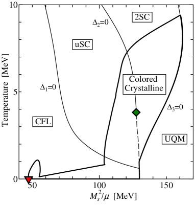
Figure 19: The unstable region in which at least one gluon has imaginary Meissner mass is shown enclosed with solid thick lines, which can be interpreted as boundaries between the homogeneous and (colored) crystalline phases.

Our approach here is essentially along the same line as in Ref. Fukushima:2004zq , and so this work leaves the same open questions enumerated in Ref. Fukushima:2004zq ; how gauge field fluctuations affect the critical point and the order of respective phase transitions Matsuura:2003md , what the nature of $K^{0}$-condensation in the gCFL phase is and how it affects instability Kryjevski:2004jw ; Buballa:2004sx , what difference the ’t Hooft (instanton) interaction makes that induces an interaction like $\sim|\Delta_{3}|^{2}M_{s}$, where the chiral phase transition is located and how our ($M_{s}^{2}/\mu$-$T$) phase diagram is mapped onto the ($\mu$-$T$) plane with $M_{s}$ solved dynamically.

In addition to these above mentioned issues, we should make an improvement how to take account of $M_{s}$ fully. The derivation of our formula (69) needs the energy projection operator for massless quarks and works out as long as the $M_{s}$ effects can be well-approximated by a chemical potential shift. From this reason, we could not augment the phase diagrams for stronger couplings (Figs. 16 and 17 in Ref. Fukushima:2004zq for example) with the instability lines. The improvement could be implemented by the full angle-integration in $\boldsymbol{p}$ to acquire $\Omega_{A}$.

From the theoretical point of view, logarithmic divergences that have been simply neglected in the present work must be taken seriously. In particular, logarithmic terms depending on $M_{s}$ seem to remain even in the normal phase Alford , while in our work the Meissner masses turn out to be zero properly in the normal phase, suggesting some cancellation mechanism between $M_{s}$ dependent divergences. This must be further investigated in a field-theoretical way. Another problem of theoretical interest is how much singularities are inhibited by non-perturbative resummation. However small the coupling constant $g$ is, the polarization is divergently large at the one-loop level, and generally, that demands a sort of resummation, for instance, by means of the ladder approximation. The instability might not be cured itself by resummation, but the singularities near the gCFL onset would be possibly smoothened.

Phenomenologically, since not only the gCFL but also the g2SC phase is within our scope especially once we will be able to approach the stronger coupling case, it is inevitable to examine the competition between the mixed and crystalline phases around the g2SC region. The entanglement between these phase possibilities should play an important role to complement the phase diagram for the large $M_{s}$ or moderate density region iida .

- (1) For reviews, see K. Rajagopal and F. Wilczek, arXiv:hep-ph/0011333; M. G. Alford, Ann. Rev. Nucl. Part. Sci. 51, 131 (2001) [arXiv:hep-ph/0102047]; G. Nardulli, Riv. Nuovo Cim. 25N3, 1 (2002) [arXiv:hep-ph/0202037]; S. Reddy, Acta Phys. Polon. B 33, 4101 (2002) [arXiv:nucl-th/0211045]; T. Schäfer, arXiv:hep-ph/0304281; M. Alford, Prog. Theor. Phys. Suppl. 153, 1 (2004) [arXiv:nucl-th/0312007]; M. Huang, arXiv:hep-ph/0409167.
- (2) M. G. Alford, K. Rajagopal and F. Wilczek, Nucl. Phys. B 537, 443 (1999) [arXiv:hep-ph/9804403].
- (3) K. Iida and G. Baym, Phys. Rev. D 63, 074018 (2001) [Erratum-ibid. D 66, 059903 (2002)] [arXiv:hep-ph/0011229].
- (4) M. Alford and K. Rajagopal, JHEP 0206, 031 (2002) [arXiv:hep-ph/0204001].
- (5) A. W. Steiner, S. Reddy and M. Prakash, Phys. Rev. D 66, 094007 (2002) [arXiv:hep-ph/0205201].
- (6) K. Rajagopal and F. Wilczek, Phys. Rev. Lett. 86, 3492 (2001) [arXiv:hep-ph/0012039].
- (7) S. B. Ruster, I. A. Shovkovy and D. H. Rischke, Nucl. Phys. A 743, 127 (2004) [arXiv:hep-ph/0405170].
- (8) K. Fukushima, C. Kouvaris and K. Rajagopal, Phys. Rev. D 71, 034002 (2005) [arXiv:hep-ph/0408322].
- (9) M. Alford, C. Kouvaris and K. Rajagopal, Phys. Rev. Lett. 92, 222001 (2004) [arXiv:hep-ph/0311286]; Phys. Rev. D 71, 054009 (2005) [arXiv:hep-ph/0406137].
- (10) A. I. Larkin and Yu. N. Ovchinnikov, Sov. Phys. JETP 20, 762 (1965); P. Fulde and R. A. Ferrell, Phys. Rev. 135, A550 (1964).
- (11) M. G. Alford, J. A. Bowers and K. Rajagopal, Phys. Rev. D 63, 074016 (2001) [arXiv:hep-ph/0008208].
- (12) G. Sarma, J. Phys. Chem. Solids 24, 1029 (1963).
- (13) M. G. Alford, J. Berges and K. Rajagopal, Phys. Rev. Lett. 84, 598 (2000) [arXiv:hep-ph/9908235].
- (14) E. Gubankova, W. V. Liu and F. Wilczek, Phys. Rev. Lett. 91, 032001 (2003) [arXiv:hep-ph/0304016].
- (15) M. M. Forbes, E. Gubankova, W. V. Liu and F. Wilczek, Phys. Rev. Lett. 94, 017001 (2005) [arXiv:hep-ph/0405059].
- (16) M. Huang and I. Shovkovy, Phys. Lett. B 564, 205 (2003) [arXiv:hep-ph/0302142]; Nucl. Phys. A 729, 835 (2003) [arXiv:hep-ph/0307273].
- (17) F. Neumann, M. Buballa and M. Oertel, Nucl. Phys. A 714, 481 (2003) [arXiv:hep-ph/0210078].
- (18) I. Shovkovy, M. Hanauske and M. Huang, Phys. Rev. D 67, 103004 (2003) [arXiv:hep-ph/0303027].
- (19) P. F. Bedaque, H. Caldas and G. Rupak, Phys. Rev. Lett. 91, 247002 (2003) [arXiv:cond-mat/0306694].
- (20) S. Reddy and G. Rupak, Phys. Rev. C 71, 025201 (2005) [arXiv:nucl-th/0405054].
- (21) M. Alford, C. Kouvaris and K. Rajagopal, arXiv:hep-ph/0407257.
- (22) M. Alford, P. Jotwani, C. Kouvaris, J. Kundu and K. Rajagopal, arXiv:astro-ph/0411560.
- (23) M. Huang and I. A. Shovkovy, Phys. Rev. D 70, 051501 (2004) [arXiv:hep-ph/0407049]; Phys. Rev. D 70, 094030 (2004) [arXiv:hep-ph/0408268].
- (24) R. Casalbuoni, R. Gatto, M. Mannarelli, G. Nardulli and M. Ruggieri, Phys. Lett. B 605, 362 (2005) [Erratum-ibid. B 615, 297 (2005)] [arXiv:hep-ph/0410401].
- (25) M. Alford and Q. h. Wang, J. Phys. G: Nucl. Part. 31, 719 (2005) [arXiv:hep-ph/0501078].
- (26) M. Huang, arXiv:hep-ph/0504235.
- (27) I. Giannakis and H. C. Ren, Phys. Lett. B 611, 137 (2005) [arXiv:hep-ph/0412015]; arXiv:hep-th/0504053.
- (28) H. Abuki, M. Kitazawa and T. Kunihiro, arXiv:hep-ph/0412382; S. B. Ruster, V. Werth, M. Buballa, I. A. Shovkovy and D. H. Rischke, arXiv:hep-ph/0503184; D. Blaschke, S. Fredriksson, H. Grigorian, A. M. Oztas and F. Sandin, arXiv:hep-ph/0503194.
- (29) P. Amore, M. C. Birse, J. A. McGovern and N. R. Walet, Phys. Rev. D 65, 074005 (2002) [arXiv:hep-ph/0110267].
- (30) D. H. Rischke, Phys. Rev. D 62, 034007 (2000) [arXiv:nucl-th/0001040]; Phys. Rev. D 62, 054017 (2000) [arXiv:nucl-th/0003063].
- (31) A. Schmitt, Q. Wang and D. H. Rischke, Phys. Rev. D 69, 094017 (2004) [arXiv:nucl-th/0311006].
- (32) D. T. Son and M. A. Stephanov, Phys. Rev. D 61, 074012 (2000) [arXiv:hep-ph/9910491]; Phys. Rev. D 62, 059902 (2000) [arXiv:hep-ph/0004095].
- (33) M. Alford and Q. h. Wang, in private communications.
- (34) J. I. Kapusta, Finite-temperature field theory, (Cambridge, Cambridge Univ. Press, 1989).
- (35) T. Matsuura, K. Iida, T. Hatsuda and G. Baym, Phys. Rev. D 69, 074012 (2004) [arXiv:hep-ph/0312042]; I. Giannakis, D. f. Hou, H. c. Ren and D. H. Rischke, Phys. Rev. Lett. 93, 232301 (2004) [arXiv:hep-ph/0406031].
- (36) A. Kryjevski and T. Schafer, Phys. Lett. B 606, 52 (2005) [arXiv:hep-ph/0407329]; A. Kryjevski and D. Yamada, Phys. Rev. D 71, 014011 (2005) [arXiv:hep-ph/0407350].
- (37) M. Buballa, Phys. Lett. B 609, 57 (2005) [arXiv:hep-ph/0410397]; M. M. Forbes, arXiv:hep-ph/0411001.
- (38) K. Iida, in private communications.