NRQCD Factorization and Universality of NRQCD Matrix Elements

J.P. Ma

Institute of Theoretical Physics , Academia Sinica, Beijing 100080, China    

Department of Physics, Shandong University, Jinan Shandong 250100, China

Z.G. Si

Department of Physics, Shandong University, Jinan Shandong 250100, China

Abstract

The approach of nonrelativistic QCD(NRQCD) factorization was proposed to study inclusive production of a quarkonium. It is widely used and successful. However, a recent study of gluon fragmentation into a quarkonium at two-loop level shows that the factorization is broken. It is suggested that the color-octet NRQCD matrix elements should be modified by adding a gauge link to restore the factorization. The modified matrix elements may have extra soft-divergences at one-loop level which the unmodified can not have, and this can lead to a violation of the universality of these matrix elements. In this letter, we examine in detail the NRQCD factorization for inclusive quarkonium production in $e^{+}e^{-}$ annihilation at one-loop level. Our results show that the factorization can be made without the modification of NRQCD matrix elements and it can also be made for relativistic corrections. It turns out that the suggested gauge link will not lead to nonzero contributions to color-octet NRQCD matrix elements at one-loop level and at any order of $v$. Therefore the universality holds at least at one-loop level.

A quarkonium system provide a unique place to study the dynamics of QCD, because a quarkonium mainly consists of a heavy quark pair $Q\bar{Q}$ and they move with a small velocity $v$. An extensive review of quarkonium physics can be found in [1]. A decade ago the approach of NRQCD factorization was proposed to study inclusive production of a quarkonium[2]. In this approach the production of a $Q\bar{Q}$ pair can be studied with perturbative QCD because the mass $m$ of $Q$ provides a large scale, the formation of the $Q\bar{Q}$ pair into a quarkonium is characterized with NRQCD matrix elements by an expansion in $v$. In order to have prediction power these matrix elements should be universal, i.e., they do not depend on how the $Q\bar{Q}$ pair is produced. This leads to the NRQCD factorization. This approach is widely used and successful. Especially, it can systematically take higher Fock state components of a quarkonium, including those components which contain a heavy quark pair in color-octet, into account. A striking success of the approach is to explain the $\psi^{\prime}$ anomaly at Tevatron [3] by taking color-octet components into account[4].

Although the approach is successful, a complete proof of the factorization does not exist. Studies of various processes at one-loop level really show that the factorization hold at one-loop level[5, 6, 7, 8, 9, 10]. But a recent study shows that the factorization for gluon fragmentation into a quarkonium at two-loop level is incomplete, indicated by that some uncancelled infrared(I.R.) divergences are not matched by NRQCD matrix elements. To restore the factorization, a gauge link is introduced to modify color-octet NRQCD matrix elements for matching these I.R. divergences[11]. At one-loop level, this gauge link can generate some extra I.R. divergences in the modified matrix elements than those unmodified. This can affect the factorization at one-loop level in the cases studied before and can lead to a violation of the universality of color-octet NRQCD matrix elements.

It is the purpose of the letter to examine if the universality is lost and if the factorization can be done in inclusive production of a quarkonium through $e^{+}e^{-}$-annihilation through a color-octet $Q\bar{Q}$ pair. Our analysis includes not only the leading contributions in the $v$-expansion, but also the contribution from relativistic corrections at order of $v^{2}$. We show at one-loop level in detail how soft divergences are cancelled or matched by color-octet NRQCD matrix elements without the gauge link suggested in [11]. Our study also shows that the relativist correction for a color-octet $Q\bar{Q}$ pair can also be factorized in the same way. To our knowledge, there is no known example studied at one-loop level to show that the NRQCD factorization holds.

We consider the inclusive production of a quarkonium $H$ in the process

$$e^{+}e^{-}\rightarrow\gamma^{*}\rightarrow H+X,$$ (1)

where the virtual photon is with the momentum $q_{\gamma}$ and $q^{2}_{\gamma}$ is much larger than the square of the quarkonium mass. For this process we need to calculate the tensor

$$T^{\mu\nu}(P,q_{\gamma},H)=\sum_{X}\int d^{4}xe^{iq_{\gamma}\cdot x}\langle 0|J^{\nu}(0)|H(P)+X\rangle\langle H(P)+X|J^{\mu}(x)|0\rangle$$ (2)

where the quarkonium carries $P$ and $J^{\mu}$ is the electric current. The NRQCD factorization in [2] suggests the tensor can be written in a factorized form:

$$T^{\mu\nu}(P,q_{\gamma},H) = F^{\mu\nu}(^{1}S_{0})\cdot\langle 0|O_{8}(^{1}S_{0},H)|0\rangle+G^{\mu\nu}(^{1}S_{0})\cdot\langle 0|P_{8}(^{1}S_{0},H)|0\rangle$$ (3)

$$+F^{\mu\nu}(^{3}P_{0})\cdot\langle 0|O_{8}(^{3}P_{0},H)|0\rangle+F^{\mu\nu,ijkl}(^{3}P_{2})\cdot\langle 0|O_{8}^{\{ij\},\{kl\}}(^{3}P_{2},H)|0\rangle+\cdots,$$

where the matrix elements in the right hand side are defined with NRQCD fields and can be found in [2]. We only consider the production through those color-octet channels which can be at the leading order of $\alpha_{s}$, i.e., the channel with the quantum number ${}^{1}S_{0}$ and ${}^{3}P_{J}$ with $J=0,2$. There is a velocity-power counting rule to determine the relative importance of NRQCD matrix elements[12, 2] for a given quarkonium. In the factorized form the second term is for the relativistic correction of the channel ${}^{1}S_{0}$. The coefficients in the front of the NRQCD matrix elements can be calculated with perturbative QCD, they are series in $\alpha_{s}$, e.g.,

$$G^{\mu\nu}(^{1}S_{0})=G_{0}^{\mu\nu}(^{1}S_{0})+G_{1}^{\mu\nu}(^{1}S_{0})+\cdots,$$ (4)

where the subscriber $0(1)$ stand for the tree(one-loop) contribution. If the factorization holds, these perturbative coefficients should not contain any I.R. divergence. To determine these coefficients, one replaces the quarkonium $H$ with a $Q\bar{Q}$ state and calculates $T^{\mu\nu}$ and the NRQCD matrix elements. By comparing both sides of Eq.(3) calculated with the $Q\bar{Q}$ pair the perturbative coefficients can be extracted. If the factorization holds, soft divergences in $T^{\mu\nu}$ will have the same form as those appearing in the matrix elements so that the perturbative coefficients do not contain any soft divergence.

To study the factorization we need to calculate the tensor $T^{\mu\nu}$ in perturbative theory after replacing the quarkonium $H$ with those $Q\bar{Q}$ states:

$$T^{\mu\nu}(P,q_{\gamma},Q\bar{Q})=\sum_{X}\int d^{4}xe^{iq_{\gamma}\cdot x}\langle 0|J^{\nu}(0)|Q(p_{1}^{\prime})\bar{Q}(p_{2}^{\prime})+X\rangle\langle\bar{Q}(p_{2})Q(p_{1})+X|J^{\mu}(x)|0\rangle.$$ (5)

It should be noted that the heavy quarks carry different momenta in the amplitude and its complex conjugated. This will enable us to identify different states of the $Q\bar{Q}$ pair. These momenta are given as:

$$p_{1}=\frac{1}{2}P+q,\ \ \ \ \ \ p_{2}=\frac{1}{2}P-q,\ \ \ \ \ \ p_{1}^{\prime}=\frac{1}{2}P+q^{\prime},\ \ \ \ \ \ p_{2}^{\prime}=\frac{1}{2}P-q^{\prime}.$$ (6)

In the rest frame of the $Q\bar{Q}$, $q^{\mu}=(0,{\bf q})$ and $q^{\prime\mu}=(0,{\bf q}^{\prime})$ with ${\bf q}^{2}={\bf q}^{\prime 2}$ and

$$P^{2}=(p_{1}+p_{2})^{2}=4(m^{2}+{\bf q}^{2}),\ \ \ \ \ \ {\bf v}=\frac{{\bf q}}{m},\ \ \ \ {\bf v^{\prime}}=\frac{{\bf q^{\prime}}}{m},$$ (7)

$v(v^{\prime})$ is the velocity of the heavy quark in the rest frame. At tree level, the unobserved state $X$ contains only one gluon. By expanding ${\bf v}$ and ${\bf v^{\prime}}$ and identifying quantum numbers, one can determine four coefficients in Eq.(3), i.e.,

$$T^{\mu\nu}_{0}(P,q_{\gamma},Q\bar{Q}) = F_{0}^{\mu\nu}(^{1}S_{0})\cdot\langle 0|O_{8}(^{1}S_{0},Q\bar{Q})|0\rangle+G_{0}^{\mu\nu}(^{1}S_{0})\cdot\langle 0|P_{8}(^{1}S_{0},Q\bar{Q})|0\rangle$$ (8)

$$+F_{0}^{\mu\nu}(^{3}P_{0})\cdot\langle 0|O_{8}(^{3}P_{0},Q\bar{Q})|0\rangle+F_{0}^{\mu\nu,ijkl}(^{3}P_{2})\cdot\langle 0|O_{8}^{\{ij\},\{kl\}}(^{3}P_{2},Q\bar{Q})|0\rangle$$

$$+{\mathcal{O}}(v^{4}).$$

In the expansion in ${\bf v}$ and ${\bf v^{\prime}}$, the leading terms give contributions to $F_{0}^{\mu\nu}(^{1}S_{0})$ for the ${}^{1}S_{0}$ state, the next-to-leading terms, which are linear in ${\bf v}$ and ${\bf v^{\prime}}$ like ${\bf v}\cdot{\bf v^{\prime}}$, give contributions to $F_{0}^{\mu\nu}(^{3}P_{0})$ for the ${}^{3}P_{0}$ state and $F_{0}^{\mu\nu,ijkl}(^{3}P_{2})$ for the ${}^{3}P_{2}$ state. The next-to-next-to-leading terms are proportional either to the tensor $v^{i}v^{j}$ or to $v^{\prime i}v^{\prime j}$. One can decompose the tensor $v^{i}v^{j}$ or to $v^{\prime i}v^{\prime j}$ into the component of the $S$-wave with $l=0$ and of the $D$-wave with $l=2$. The $S$-wave component corresponds to the relativistic correction of the ${}^{1}S_{0}$ state. At tree level all these coefficients are nonzero and contain no soft divergence, their detailed forms are not important for our purpose because we will show that the soft-divergent correction at one-loop to these coefficients is proportional to the tree-level result $T^{\mu\nu}_{0}$. We will use Feynman gauge in this letter. In this gauge one can clearly see how soft divergences are cancelled or matched in a diagram-by-diagram manner.

One-loop corrections consist of two parts. One is the virtual correction, another is the real correction in which the unobserved state $X$ contains two gluons or a light quark pair. Beside corrections from wave-function renormalization there are many Feynman diagrams. Since we are only interested in soft divergences, we do not need to consider all diagrams but only those containing soft divergences. The diagrams with soft divergences are given in Fig.1.. To obtain the soft-divergent parts of these diagrams we employ the eikonal approximation with some modification.

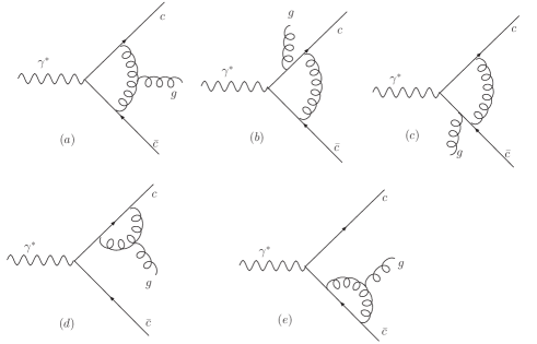
Figure 1: Diagrams for contributions containing soft divergences.

To illustrate the eikonal approximation used here, we consider the contribution from Fig.1a to the matrix element $R^{\mu}=\langle\bar{Q}(p_{2})Q(p_{1}),G(k,\varepsilon^{*},a)|J^{\mu}(x)|0\rangle$:

$$R^{\mu}_{1a} = \int\frac{d^{4}k_{1}}{(2\pi)^{4}}\bar{u}(p_{1})(-ig_{s}T^{b}\gamma^{\rho})\frac{\gamma\cdot(p_{1}+k_{1})+m}{(p_{1}+k_{1})^{2}-m^{2}}(-ieQ\gamma^{\mu})\frac{\gamma\cdot(-k_{2}-p_{2})+m}{(p_{2}+k_{2})^{2}-m^{2}}(-ig_{s}T^{c}\gamma^{\sigma})v(p_{2})$$ (9)

$$\cdot\frac{1}{k_{1}^{2}}\frac{1}{k_{2}^{2}}(-g_{s}f^{abc})\left[(-k-k_{1})_{\sigma}\varepsilon^{*}_{\rho}+(k_{1}-k_{2})\cdot\varepsilon^{*}g_{\rho\sigma}+(k_{2}+k)_{\rho}\varepsilon^{*}_{\sigma}\right],$$

with $k_{2}=k-k_{1}$. The soft divergence appears when $k_{1}$ or $k_{2}$ becomes soft, i.e., all components of $k_{1}$ or $k_{2}$ becomes small, and when $k_{1}$, hence also $k_{2}$, is collinear to the momentum $k$ of the outgoing gluon. If the gluon with $k_{1}$ is soft, the standard approximation is to neglect all $k_{1}$ in nominators and keep only the leading order in $k_{1}$ in the denominators. Therefore the contribution from the soft region of $k_{1}$ can be written as:

$$R^{\mu}_{1a,s1} = -ieQg_{s}^{3}\int\frac{d^{4}k_{1}}{(2\pi)^{4}}\bar{u}(p_{1})f^{abc}T^{b}T^{c}\frac{2p_{1}^{\rho}}{2p_{1}\cdot k_{1}}\gamma^{\mu}\frac{\gamma\cdot(-p_{2}-k)+m}{2p_{2}\cdot k}\gamma^{\sigma}v(p_{2})$$ (10)

$$\cdot\frac{1}{k_{1}^{2}}\cdot\frac{1}{(-2k_{1}\cdot k)}\cdot\left[-k_{\sigma}\varepsilon_{\rho}^{*}-k\cdot\varepsilon^{*}g_{\rho\sigma}+2k_{\rho}\varepsilon^{*}_{\sigma}\right].$$

We use dimensional regularization with $d=4-\epsilon$ to regularize divergences. The pole with $1/\epsilon_{I}$ is for I.R. divergence with $\epsilon_{I}=4-d$. Other poles without the subscriber $I$ are for U.V. divergences. Calculating the integral we find that the soft amplitude contains double pole in the form $\epsilon^{-1}(\epsilon^{-1}-\epsilon^{-1}_{I})$, indicating that the approximation may not be convenient here. A convenient approximation we will use is to keep denominators exact. With this approximation, the soft- and collinear-divergent part of the contribution can be written as

$$R^{\mu}_{1a,sc} = -ieQg_{s}^{3}\int\frac{d^{4}k_{1}}{(2\pi)^{4}}\frac{1}{(2p_{1}\cdot k_{1}+i0)(2p_{2}\cdot k_{2}+i0)(k_{1}^{2}+i0)(k_{2}^{2}+i0)}$$ (11)

$$\bar{u}(p_{1})f^{abc}T^{b}T^{c}\left[(2p_{1}^{\rho}+\gamma^{\rho}\gamma^{+}k_{1}^{-})\gamma^{\mu}(-2p_{2}^{\sigma}-k_{2}^{-}\gamma^{+}\gamma^{\sigma})\right]v(p_{2})$$

$$\left[(-k-k_{1})^{-}n_{\sigma}\varepsilon^{*}_{\rho}+(2k_{1}-k)^{-}n\cdot\varepsilon^{*}g_{\rho\sigma}+(k_{2}+k)^{-}n_{\rho}\varepsilon^{*}_{\sigma}\right],$$

and $R^{\mu}_{1a}-R^{\mu}_{1a,sc}$ contains no any soft divergence. In the above equation we have taken a frame in which

$$k^{\mu}=(0,k^{-},0,0)=k^{-}n^{\mu},\ \ \ \ \ \ q^{\mu}_{\gamma}=(q_{\gamma}^{+},q^{-}_{\gamma},0,0).$$ (12)

It should be noted that $R^{\mu}_{2a,sc}$ can be written in a covariant form. Performing a similar analysis for other diagrams and loop-momentum integration we obtain the soft-divergent part of the one-loop correction to $R^{\mu}$. The sum of contributions from Fig.1a, Fig.1d and Fig.1e can be written in a compact form:

$$R^{\mu}_{1a,sc}+R^{\mu}_{1d,sc}+R^{\mu}_{1e,sc} = \frac{ieQg_{s}^{3}}{(4\pi)^{2}}N_{c}\left\{2\left(\frac{2}{\epsilon_{I}}\right)^{2}-\frac{2}{\epsilon_{I}}\left[2\gamma-2+\ln\frac{(2p_{1}\cdot k)^{2}}{4\pi m^{2}\mu^{2}}+\ln\frac{(2p_{2}\cdot k)^{2}}{4\pi m^{2}\mu^{2}}\right]\right\}$$ (13)

$$\cdot\bar{u}(p_{1})T^{a}\left[\gamma^{\nu}\frac{\gamma\cdot(p_{1}+k)+m}{(p_{1}+k)^{2}-m^{2}}\gamma^{\mu}+\gamma^{\mu}\frac{\gamma\cdot(-p_{2}-k)+m}{(p_{2}+k)^{2}-m^{2}}\gamma^{\nu}\right]v(p_{2}),$$

i.e., the soft-divergent part is proportional to the tree-level amplitude. The double pole in $\epsilon_{I}$ is from the overlap of collinear- and soft region of the loop momentum. The contribution from Fig.1b and Fig.1c contain not only soft divergences but also Coulomb singularities. With our approximation the sum of these two diagrams gives:

$$R^{\mu}_{2b,cs}+R^{\mu}_{2c,cs} = \frac{ieQg_{s}^{3}}{(4\pi)^{2}}\frac{1+2v^{2}}{N_{c}}\left[\frac{\pi^{2}}{2v}+\frac{2}{\epsilon_{I}}\left(1-\frac{2v^{2}}{3}\right)\right]$$ (14)

$$\cdot\varepsilon^{*}_{\nu}\bar{u}(p_{1})T^{a}\left[\gamma^{\nu}\frac{\gamma\cdot(p_{1}+k)+m}{(p_{1}+k)^{2}-m^{2}}\gamma^{\mu}+\gamma^{\mu}\frac{\gamma\cdot(-p_{2}-k)+m}{(p_{2}+k)^{2}-m^{2}}\gamma^{\nu}\right]v(p_{2})+\cdots,$$

where $\cdots$ stand for terms which are finite with $\epsilon,v\rightarrow 0$, and higher orders in $v$.

Putting everything together, we obtain the soft divergent part of the virtual one-loop contribution to $T^{\mu\nu}$ in Feynman gauge:

$$T_{1,\ vir.}^{\mu\nu}(P,q_{\gamma},Q\bar{Q}) = -\frac{\alpha_{s}}{2\pi}\frac{1}{N_{c}}\left[\frac{2}{\epsilon_{I}}\left(1+\frac{2}{3}v^{2}+\frac{2}{3}v^{\prime 2}+{\mathcal{O}}(v^{4})\right)+\frac{\pi^{2}}{2v}(1+{\mathcal{O}}(v^{2}))\right]T_{0}^{\mu\nu}(P,q_{\gamma},Q\bar{Q})$$

$$-\frac{\alpha_{s}}{2\pi}N_{c}\left[\left(\frac{2}{\epsilon_{I}}\right)^{2}-\frac{2}{\epsilon_{I}}\left(\gamma-1+L_{n}\right)\right]T_{0}^{\mu\nu}(P,q_{\gamma},Q\bar{Q})$$

$$-\frac{\alpha_{s}}{2\pi}\left(\frac{2}{\epsilon_{I}}\right)\left[\frac{N_{c}^{2}-1}{N_{c}}+\left(\frac{5}{6}N_{c}-\frac{1}{3}N_{f}\right)\right]T_{0}^{\mu\nu}(P,q_{\gamma},Q\bar{Q})+\cdots$$

$$L_{n} = \frac{1}{2}\ln\frac{(p_{1}\cdot k)(p_{1}^{\prime}\cdot k)(p_{2}\cdot k)(p_{2}^{\prime}\cdot k)}{(\pi m^{2}\mu^{2})^{2}},$$ (15)

where $\cdots$ denote finite parts and the correction terms in the third line come from wave-function renormailization of the heavy quarks and the gluon.

Now we turn to the real correction. The real correction consists of amplitudes of two gluons or a light quark pair. The two gluons can be emitted by heavy quarks and by gluon splitting, the light quark pair can only be generated through gluon splitting. It should be noted that a light quark pair can also be produced in other ways, but the contribution of this is irrelevant for the factorization discussed here, because in this case the heavy quark pair is in states other than those given in Eq.(8) and the contribution at order $\alpha_{s}^{2}$ is free from soft divergences. The Feynman diagrams for the real correction is given in Fig.2.

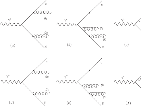
Figure 2: Real correction

We write the amplitude with two gluons in the final state as

$$R^{\mu}_{gg}=R^{\mu}_{gg,Q}+R^{\mu}_{gg,g},$$ (16)

where the first term is only for two gluons emitted by heavy quarks and second is for gluon splitting. If two gluons are emitted by heavy quarks, there are only I.R. divergences, when one of the gluons becomes soft. Collinear singularities will not appear here because of the massive quarks. When the gluon with the momentum $k_{1}$ becomes soft, the soft contribution of $R^{\mu}_{gg,Q}$ with the standard eikonal approximation can be written:

$$R^{\mu}_{gg,Q,s}=\frac{ig_{s}}{2}f^{a_{1}a_{2}a}\left(\frac{p_{1}\cdot\varepsilon^{*}_{1}}{p_{1}\cdot k_{1}}+\frac{p_{2}\cdot\varepsilon^{*}_{1}}{p_{2}\cdot k_{1}}\right)\langle\bar{Q}(p_{2})Q(p_{1}),G(k_{2},\varepsilon_{2},a)|J^{\mu}(0)|0\rangle|_{Tree\ level}+\cdots,$$ (17)

where we only give those contributions explicitly, which are from the color-octet $Q\bar{Q}$ pair with the quantum numbers ${}^{1}S_{0}$ and ${}^{3}P_{J}$ with $J=0,2$. The contributions from states different than those above are indicated by $\cdots$. They are not important for our purpose, but they are important for the complete cancellation of soft divergences in the KLN theorem. We will discuss this later. The contribution from $R^{\mu}_{gg,Q,s}$ to $T^{\mu\nu}$ can be calculated easily, we obtain:

$$T^{\mu\nu}_{1,Q,s}(P,q_{\gamma},Q\bar{Q})=\frac{\alpha_{s}}{2\pi}N_{c}\left(\frac{2}{\epsilon_{I}}\right)\left[1+\frac{1}{3}v^{2}+\frac{1}{3}v^{\prime 2}+{\mathcal{O}}(v^{4})\right]T_{0}^{\mu\nu}(P,q_{\gamma},Q\bar{Q})+\cdots$$ (18)

where we have only collected the contributions from relevant $Q\bar{Q}$ states. Contributions from other states and higher orders of $v$ are represented by $\cdots$.

The amplitude from the gluon splitting is given by:

$$R^{\mu}_{gg,g} = eQg_{s}^{2}f^{aa_{1}a_{2}}\bar{u}(p_{1})T^{a}\left[\gamma^{\nu}\frac{\gamma\cdot(p_{1}+k)+m}{(p_{1}+k)^{2}-m^{2}}\gamma^{\mu}+\gamma^{\mu}\frac{\gamma\cdot(-p_{2}-k)+m}{(p_{2}+k)^{2}-m^{2}}\gamma^{\nu}\right]v(p_{2})$$ (19)

$$\left[(k+k_{1})\cdot\varepsilon_{2}^{*}\varepsilon^{*}_{1\nu}+(-k_{1}+k_{2})_{\nu}\varepsilon_{1}^{*}\cdot\varepsilon_{2}^{*}+(-k_{2}-k)\cdot\varepsilon_{1}^{*}\varepsilon_{2\nu}^{*}\right]\frac{1}{(k_{1}+k_{2})^{2}},$$

with $k=k_{1}+k_{2}$. The contribution from $R^{\mu}_{gg,g}$ to $T^{\mu\nu}$ is more difficult to evaluate than that from $R^{\mu}_{gg,Q}$, because there is a overlap between the collinear- and soft region of gluon momenta. However there is a standard method, called phase-space slicing method, discussed in detail in [13, 14]. We will use the method. If the gluon with $k_{1}$ is soft, the amplitude can be approximated by:

$$R^{\mu}_{gg,g,s} = eQg_{s}^{2}f^{aa_{1}a_{2}}\bar{u}(p_{1})T^{a}\left[\gamma^{\nu}\frac{\gamma\cdot(p_{1}+k_{2})+m}{(p_{1}+k_{2})^{2}-m^{2}}\gamma^{\mu}+\gamma^{\mu}\frac{\gamma\cdot(-p_{2}-k_{2})+m}{(p_{2}+k_{2})^{2}-m^{2}}\gamma^{\nu}\right]v(p_{2})$$ (20)

$$\cdot\frac{(-2k_{2}\cdot\varepsilon_{1}^{*})\varepsilon_{2\nu}^{*}}{(k_{1}+k_{2})^{2}}.$$

This amplitude $R^{\mu}_{gg,g,s}$ interfered with the $R^{\mu}_{gg,Q,s}$ will give contributions with the soft divergences which are exactly those in the contributions from the interference between $R^{\mu}_{gg,Q}$ and $R^{\mu}_{gg,g}$. By the method mentioned above we have the contribution from the interference:

$$T^{\mu\nu}_{1,int.}(P,q_{\gamma},Q\bar{Q})=\frac{\alpha_{s}}{2\pi}N_{c}\left\{\left(\frac{2}{\epsilon_{I}}\right)^{2}-\frac{2}{\epsilon_{I}}\left[\gamma+\ln\frac{s^{2}_{min}}{\pi m^{2}\mu^{2}}\right]\right\}T_{0}^{\mu\nu}(P,q_{\gamma},Q\bar{Q}),$$ (21)

where $s_{min}$ is a cut-off in the phase-space slicing method. Our final result will not depend on it. The contributions only from the gluon splitting into two gluons and a light quark pair can be calculated directly with the phase-space slicing method. They contain only collinear singularities. The result is:

$$T^{\mu\nu}_{1,col}(P,q_{\gamma},Q\bar{Q})=\frac{\alpha_{s}}{2\pi}\left(\frac{2}{\epsilon_{I}}\right)\left\{N_{c}\left[-L_{n}+\ln\frac{s^{2}_{min}}{\pi m^{2}\mu^{2}}+\frac{11}{6}\right]-\frac{N_{f}}{3}\right\}T_{0}^{\mu\nu}(P,q_{\gamma},Q\bar{Q}),$$ (22)

where the same dependence on the cut-off $s_{min}$ appears and it will be cancelled by that in $T^{\mu\nu}_{1,int.}$. Putting everything together we obtain the infrared divergent part of the real correction as:

$$T^{\mu\nu}_{1,\ real}(P,q_{\gamma},Q\bar{Q}) = \frac{\alpha_{s}}{2\pi}\left\{N_{c}\left[\left(\frac{2}{\epsilon_{I}}\right)^{2}-\frac{2}{\epsilon_{I}}\left(\gamma-1+L_{n}\right)\right]\right\}T_{0}^{\mu\nu}(P,q_{\gamma},Q\bar{Q})$$ (23)

$$+\frac{\alpha_{s}}{2\pi}\frac{2}{\epsilon_{I}}\left\{N_{c}\left[\frac{11}{6}+\frac{1}{3}v^{2}+\frac{1}{3}v^{\prime 2}\right]-\frac{N_{f}}{3}\right\}T_{0}^{\mu\nu}(P,q_{\gamma},Q\bar{Q})+\cdots,$$

Finally, we obtain the total soft-divergent part of $T^{\mu\nu}$ at one loop:

$$T_{1}^{\mu\nu}(P,q_{\gamma},Q\bar{Q}) = \frac{\alpha_{s}}{2\pi}\left[(v^{2}+v^{\prime 2})\left(\frac{2}{\epsilon_{I}}\right)\frac{N_{c}^{2}-2}{3N_{c}}-\frac{1}{N_{c}}\frac{\pi^{2}}{2v}\right]T_{0}^{\mu\nu}(P,q_{\gamma},Q\bar{Q})+\cdots,$$ (24)

where we only give the relevant part in detail. It should be noted that the $[\cdots]$ of the part does not contain ${\bf v}\cdot{\bf v^{\prime}}$ from our calculation at the orders considered here. The $\cdots$ denote contributions from other states of the $Q\bar{Q}$ pair, which can not be produced at tree-level. These contributions are from $R^{\mu}_{gg,Q}$, represented by $\cdots$ in Eq.(18), they contain terms like ${\bf v}\cdot{\bf v^{\prime}}$ because the $Q\bar{Q}$ pair at one-loop order can be in a color-singlet $P$-wave states.

Before we turn to our result of NRQCD matrix elements to finalize NRQCD factorization, we briefly discuss here the cancellation of soft divergences in KLN theorem. It should be noted that in $T^{\mu\nu}$ defined in Eq.(5) the heavy quark pair can be in an arbitrary state which is allowed to be produced at a given order of $\alpha_{s}$, i.e., we do not sum over all possible states of the heavy quark pair. If we sum all these states and take ${\bf v}={\bf v^{\prime}}$, the sum should not contain any soft divergence, as stated by KLN theorem. The sum contains not only those terms explicitly given in Eq.(24), but also those represented by $\cdots$, i.e., the contributions from those states which can not be produced at tree level, these states are produced through emission of two gluons by heavy quarks, whose contributions are represented in Eq.(18) by $\cdots$. Taking these contributions into account we have the soft-divergent part of the sum:

$$\sum T_{1}^{\mu\nu}(P,q_{\gamma},Q\bar{Q}){\Big{|}}_{{\bf v}={\bf v^{\prime}}} = \frac{\alpha_{s}}{\pi}v^{2}\left(\frac{2}{\epsilon_{I}}\right)\frac{N_{c}^{2}-2}{3N_{c}}\sum T_{0}^{\mu\nu}(P,q_{\gamma},Q\bar{Q}){\Big{|}}_{{\bf v}={\bf v^{\prime}}}$$ (25)

$$-\frac{\alpha_{s}}{\pi}v^{2}\left(\frac{2}{\epsilon_{I}}\right)\frac{N_{c}^{2}-2}{3N_{c}}\sum T_{0}^{\mu\nu}(P,q_{\gamma},Q\bar{Q}){\Big{|}}_{{\bf v}={\bf v^{\prime}}}+\cdots,$$

where the second term comes from the contributions of those states which are not given explicitly in Eq.(18). By summing of these states and some manipulation the sum can be written into a compact form as given in the above. We see clearly that the sum is free from any soft divergence as KLN theorem states.

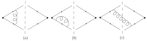
Figure 3: Examples of Feynman diagrams for (a) vertex correction, (b) wave-function renormalization and (c) gluon-exchange correction, the broken line is the cut.

The one-loop correction of those NRQCD matrix elements in Eq.(8) and Eq.(12) can be divided into two parts as a virtual part and a real part. The virtual part consists of corrections from vertex and wave-function renormailization. Examples of Feynman diagrams at one-loop level for the real part, vertex- and wave-function renormailization correction are given in Fig.3. up to the orders of $v$ we consider. We calculate these corrections in Feynman gauge. The one loop correction can be written as:

$$\langle 0|O_{n}^{Q\bar{Q}}|0\rangle_{1}=\langle 0|O_{n}^{Q\bar{Q}}|0\rangle_{0}\left[-\frac{\pi\alpha_{s}}{4v}\cdot\frac{1}{N_{c}}(1+{\mathcal{O}}(v^{2}))+{\mathcal{O}}(v^{2})\right]$$ (26)

where $O_{n}^{Q\bar{Q}}$ is any of $O_{8}(^{1}S_{0})$, $P_{8}(^{1}S_{0})$, $O(^{3}P_{J})$ with $J=0,1,2$, the matrix element with the subscriber $0(1)$ is the tree-level(one-loop) result of the operator. The first term represents the Coulomb singularity, the second term starts at the relative order of $v^{2}$, combined with $\langle 0|O_{n}^{Q\bar{Q}}|0\rangle_{0}$ they should be written in the form as matrix elements of operators. Using this result we can clearly see that the Coulomb singularity in Eq.(24) is reproduced. Hence, one can conclude that all perturbative coefficients $F^{\prime}s$ in Eq.(3) are free from the Coulomb singularity and also from I.R. divergences.

To assess if $G^{\mu\nu}(^{1}S_{0})$ contains any I.R. divergence, we need to take the operator mixing between $O_{8}(^{1}S_{0})$ and others into account which is contained in the second term in Eq.(26). At one loop and order $v^{2}$, the operator can be mixed with the color-singlet operator with quantum numbers ${}^{1}P_{1}$ and the color-octet operator $P_{8}(^{1}S_{0},Q\bar{Q})$. The later is relevant for our case. In Feynman gauge we have

$$\langle 0|O_{8}(^{1}S_{0},Q\bar{Q})|0\rangle = -\frac{\alpha_{s}}{2\pi}\frac{1}{N_{c}}\left(\frac{2}{\epsilon_{I}}\right)\left(\langle 0|O_{8}(^{1}S_{0},Q\bar{Q})|0\rangle_{0}+\frac{2}{3m^{2}}\langle 0|P_{8}(^{1}S_{0},Q\bar{Q})|0\rangle_{0}+{\mathcal{O}}(v^{4})\right)$$

$$-\frac{\alpha_{s}}{2\pi}\frac{N_{c}^{2}-1}{N_{c}}\left(\frac{2}{\epsilon_{I}}\right)\langle 0|O_{8}(^{1}S_{0},Q\bar{Q})|0\rangle_{0}$$

$$+\frac{\alpha_{s}}{2\pi}N_{c}\left(\frac{2}{\epsilon_{I}}\right)\left(\langle 0|O_{8}(^{1}S_{0},Q\bar{Q})|0\rangle_{0}+\frac{1}{3m^{2}}\langle 0|P_{8}(^{1}S_{0},Q\bar{Q})|0\rangle_{0}\right)$$

$$+\cdots,$$

$$\langle 0|P_{8}(^{1}S_{0},Q\bar{Q})|0\rangle_{0} = m^{2}(v^{2}+v^{\prime 2})\langle 0|O_{8}(^{1}S_{0},Q\bar{Q})|0\rangle_{0},$$ (27)

where contributions at orders higher than $v^{2}$ or from mixing of other irrelevant operators and those with the Coulomb singularity are represented by $\cdots$. In the above the first line comes from the vertex correction, the second from the external quark legs and the third comes from the real gluon exchange. With this result, one can see clearly how the soft divergences are absorbed into the matrix element at leading order of $v$ on a diagram-by-diagram basis. At order of $v^{0}$ all I.R. divergences are cancelled. At the next-to-leading order of $v$, the net divergence in the above equation exactly matches that in $T_{1}^{\mu\nu}$ and the matching is also on a diagram-by-diagram basis.

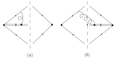
Figure 4: Types of Feynman diagrams for contributions with the gauge link. The double line stands for the gauge link. (a): Virtual correction. (b): Real correction.

Our results clearly show that without the modification of relevant NRQCD matrix elements in our case the NRQCD factorization holds at order of $v^{2}$ and the relativistic correction can also be factorized. Adding a gauge link in the those color-octet NRQCD matrix elements, as suggested in [11], the modified matrix elements will receive extra contributions. These contributions relevant for our study are given by types of Feynman diagrams in Fig.4. We use Feynman gauge to study these contributions. In other gauges, like Coulomb gauge, a gluon can also be exchanged between gauge links. By an infrared power counting each contribution from Fig.4. is with infrared divergences. The virtual contribution from the type(a) of diagrams in Fig.4, after integrating of the energy of the virtual gluon and neglecting terms which generate power divergences, is proportional to the integral:

$$\int\frac{d^{3}q}{(2\pi)^{3}}\frac{1}{2|{\bf q}|}\frac{1}{|{\bf q}|+q^{3}}\left[\frac{1+v^{3}}{-|{\bf q}|+{\bf v}\cdot{\bf q}}+\frac{1-v^{3}}{-|{\bf q}|-{\bf v}\cdot{\bf q}}\right].$$ (28)

In the above the factor $1/(|{\bf q}|+q^{3})$ comes from the eikonal propagator of the gauge link, which is determined by the moving direction of the quarkonium. We take the direction in the $z$-direction. It is clearly that the integral is infrared-divergent. But the real contribution from the type(b) of diagrams in Fig.4 is also proportional to this integral and the proportional coefficient has different sign than that of the virtual contribution. The total contribution from the gauge link to the color-octet matrix elements is zero at one loop and at any order of $v$. Therefore, at one-loop level, the suggested gauge link will not lead to a violation of the universality of color-octet matrix elements and it will not affect all existing one-loop results.

To summarize: We have examined in detail the NRQCD factorization in inclusive production of a quarkonium through $e^{+}e^{-}$-annihilation. Our results show that the factorization can be made for production of a $Q\bar{Q}$ pair in color octet with the quantum number ${}^{1}S_{0}$ and ${}^{3}P_{0,2}$ and also for relativistic correction to the $S$-wave state. The modification of color-octet NRQCD matrix elements with the suggested gauge link[11] will not affect the NRQCD factorization at one loop in cases studied before and the case studied here, because the gauge link does not lead to nonzero contributions to color-octet NRQCD matrix elements at one loop. Because of this the universality of these matrix elements holds at one loop.

Acknowledgements

The authors would like to thank Prof. J.W. Qiu for communications about the recent work[11] and Prof. G. Bodwin for intensive discussions, which greatly help to understand the problem studied here. The warm hospitality of the Taipei Summer Institute of NCTS/TPE at the Physics Department of NTU, where the first draft of the paper is completed, is acknowledged. This work is supported by National Nature Science Foundation of P. R. China.

References

• [1] N. Brambilla, et al., Quarkonium Working Group, hep-ph/0412148.
• [2] G.T. Bodwin, E. Braaten and G.P. Lepage, Phys. Rev. D51 (1995) 1125, D55 (1997) 5855(E) .
• [3] F. Abe et al., CDF Collaboration, Phys. Rev. Lett. 79, (1997), 572, Phys. Rev. Lett. 79, (1997), 578,
• [4] E. Braaten and S. Fleming, Phys. Rev. Lett. 74, (1995), 3327.
• [5] J.P. Ma, Nucl. Phys. B447 (1995) 405
• [6] E. Braaten and Y.Q. Chen, Phys. Rev. D55 (1997) 7152
• [7] E. Braaten and J. Lee, Nucl.Phys. B586 (2000) 427, J. Lee, hep-ph/0504285.
• [8] A. Petrelli, et.al., Nucl. Phys. B514 (1998) 245
• [9] M. Beneke, F. Maltoni and I.Z. Rothstein, Phys. Rev. D59 (1999) 054003
• [10] M. Klasen, B.A. Kniehl, L.N. Mihaila and M. Steinhauser, Nucl. Phys. B713 (2005) 487, Phys. Rev. D71 (2005) 014016
• [11] G.C. Nayak, J.W. Qiu, G. Sterman, Phys. Lett. B613 (2005) 45
• [12] G.P. Lepage, L. Magnea, C. Nakhleh, U. Magnea and K. Hornbostel, Phys. Rev. D46, (1992), 4052.
• [13] A. Brandenburg and P. Uwer, Nucl. Phys. B515 (1998) 279
• [14] W.T. Giele and E.W.N. Glover, Phys. Rev. D46 (1992) 1980