QCD THEORY AT THE XL RENCONTRE DE MORIOND:
FISH EYES AND PHYSICS

I review a selection of the talks at the QCD Session of the XL Rencontre de Moriond, talks either by theorists or else of special theoretical interest. I use the talks to provide some assessment of where we stand with respect to the problems and opportunities facing QCD theory.

1 Introduction

The theory of the strong interactions is well understood in one sense: we are confident that the simple lagrangian of Quantum Chromodynamics (QCD) provides the correct description of the strong interactions. After all, it has passed many experimental tests that could have proven it wrong. Yet we face challenges in applying that theory. Predictions for bound state masses are difficult, as are predictions for decays of mesons containing a heavy quark, where we need the QCD part of the theory in order to use experimental results to get at the electroweak part. There appears to be a deep simplicity in the behavior of densely packed gluons, as probed at “small x,” but this behavior is not well understood. Interesting regularities in the development of the final state in heavy ion collisions have been observed, but have not been susceptible to a fully satisfactory interpretation in terms of quark-gluon interactions. Finally, we seek more powerful tools for using the theory in the context of high $p_{T}$ reactions at the upcoming Large Hadron Collider (LHC). Surely, we imagine, new physics signals will be found there, but understanding what those signals mean in terms of new particles or forces – maybe even new dimensions of space-time – will not be easy. We will want to use all of the theoretical methods we can muster.

These issues and more came up at the conference. In this talk, I review a selection of the talks that were either presented by theorists or were of special theoretical interest. I use the talks to provide some assessment of where we stand with respect to the problems and opportunities facing QCD theory. You have to read to the end to find out about the fish part.

2 b-quark production

In the bad old days, around Moriond XXX, the data on b-quark production indicated a problem, as illustrated on the left in Fig. 1. The results varied somewhat according to year, what was measured, and how the measurement was performed, but always indicated the observation of more $b$-quarks than theory predicted. One could hide behind the excuse that the $P_{T}$ values were never more than about 20 GeV and the mass of the $b$-quark itself is only 5 GeV, so that the effective $\alpha_{s}$ was not so small and the effectiveness of the perturbative QCD approach could be doubted. Nevertheless, one was left with the suspicion that the $b$ quark had some kind of anomalous behavior that lay beyond the Standard Model. In the last few years, the situation has been changing. At this conference, M. d’Onofrio presented the latest CDF and D0 data on this subject.$\!{}^{{\bf?}}$ I present one of the results on the right in Fig. 1. We see that the theory errors are still rather substantial, reflecting the difficulties mentioned above. The experimental errors are improved. And now data and theory agree.

There was some discussion at the conference of what had changed. First, we have better theory that sums logs of $p_{T}/m_{b}$. Second, we have better parton distributions and accompanying parton distributions. (See d’Onofrio’s talk.) Third, we measure a quantity whose definition does not involve too much theory, for example we measure cross sections for B-hadron production instead of b-quark production as was sometimes done in the past. A recent trend has been to measure the cross section for jets containing a b-quark. Examples of this were shown, although so far the NLO theory calculations are lacking and summing logarithms of $p_{T}/m_{b}$ will be needed to supplement a purely NLO calculation.

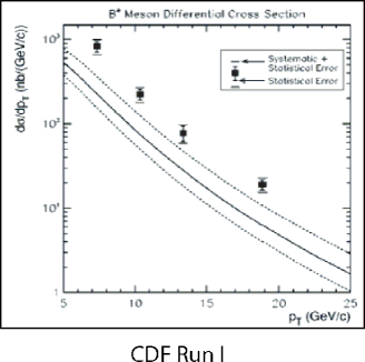
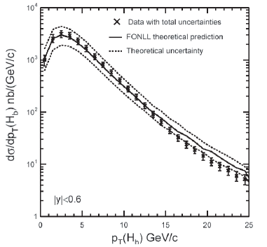
Figure 1: On the left, CDF data from about 1995 for $B^{+}$ meson production cross section versus $P_{T}$ from the talk of I. Baliev.$\!{}^{{\bf?}}$ On the right, current CDF data for B hadron production from the talk of M. d’Onofrio.$\!{}^{{\bf?}}$

3 b-quark decays

There were several talks concerning the theory of b-quark decays. These talks concerned perturbative calculations of the effective lagrangian, lattice gauge theory calculations of decay matrix elements, and theoretical analyses of the decay spectrum in inclusive decays.

The issue of the effective lagrangian is illustrated in Fig. 2. Loop diagrams create an effective lagrangian of the form

$${\cal L}=\sum C_{i}{\cal O}_{i}$$ (1)

for the process $b\to se^{+}e^{-}$ (for example). The ${\cal O}_{i}$ are operators such as $\bar{s}(x)\gamma^{\mu}b(x)\,\bar{e}(x)\gamma_{\mu}e(x)$. The coefficients $C_{i}$ are to be calculated from the loop diagrams. My example diagram is too simple; what we need now are two loop diagrams. T. Huber reported his calculation of the $C_{i}$ for $b\to se^{+}e^{-}$ from two loop diagrams in the Standard Model.$\!{}^{{\bf?}}$ S. Schilling described a calculation of the $C_{i}$ for $b\to se^{+}e^{-}$ in the case of the two higgs doublet model.$\!{}^{{\bf?}}$

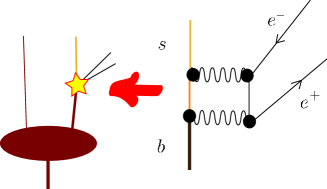
Figure 2: The effective Lagrangian for b-quark decay. The loop diagram illustrated creates an effective point interaction for $b\to se^{+}e^{-}$ since the momentum in the loop is of order $M_{W}$, which is much larger than $m_{b}$. This point interaction can then be used in a calculation of B meson decay.

If we wish to calculate a completely inclusive decay rate, not much is needed beyond the effective lagrangian for the decay. But if we want an exclusive decay rate, we need a matrix element of the effective lagrangian between initial and final states, as illustrated in Fig. 3. M. Okamoto presented results for the matrix elements of appropriate weak decay operators between an initial heavy meson state and a final light meson state.$\!{}^{{\bf?}}$ The results are needed for a range of momentum transfers $q$ to the quark system. With appropriate limiting procedures, such matrix elements can be evaluated in lattice QCD. In the calculations described by Okamoto, enough results can be obtained to extract the complete CKM matrix from the corresponding experimental results.

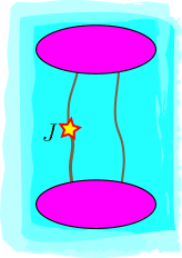
Figure 3: Calculation of the matrix element for a heavy meson decay using lattice gauge theory. Here $J$ stands for the quark part of one of the operators ${\cal O}_{i}$ in Eq. (1). The operator changes a heavy quark to a light quark and we need its matrix element between meson states.

I turn now to the decay spectrum in inclusive decays. Consider, in particular, the decay $B\to X_{s}\gamma$, where $X_{s}$ indicates any state that has an $s$-quark in it. Let $x=2E_{\gamma}/M_{b}$. From a theoretical point of view, by far the simplest cross section to calculate is the inclusive cross section $\int dx\,d\varGamma/dx$. However, the experimental acceptance typically does not include all $x$. For this reason, we need theory for $d\varGamma/dx$ as a function of $x$. In the simplest approximation, the $b$ quark in a $B$ meson carries all of the four-momentum of the meson and decays into a two body state $s\gamma$. Then $d\varGamma/dx=\delta(1-x)$. In a more realistic picture, we expect the photon spectrum to be spread out, as illustrated in the left-hand part of Fig. 4. If one calculates Feynman diagrams like the simple one in the right-hand part of Fig. 4, one gets contributions that are singular at $x\to 1$ (before smearing by the wave function). In the region $(1-x)\ll 1$, one can sum a series containing more and more powers of $\log(1-x)$. However, this series does not converge well. E. Gardi $\!{}^{{\bf?}}$ reported on this. He blamed the bad behavior of the perturbative series on an infrared renormalon, which is associated with a factor of $n!$ at $n$th order in perturbation theory. The simple way to understand this is that diagrams like that illustrated on the right in Fig. 4 get contributions from the region in which the loop momentum $l$ is smaller than, say, 1 GeV. The $n!$ factor is the price we pay for applying perturbation theory in a region in which perturbation theory does not really apply.

Of course, this kind of behavior is generic in QCD perturbation theory. However, the renormalon behavior is particularly bothersome in this instance. Gardi reported that the bad behavior stems from the use of the “pole mass” in the heavy quark propagator. With a reorganized calculation, he reported that the integration is less sensitive to the infrared region and the predictive power of the theory can be improved.

         

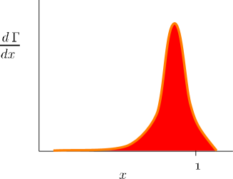
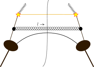
Figure 4: Left: sketch of the behavior of the differential decay width for $B\to X_{s}\gamma$ as a function of $x=2E_{\gamma}/M_{b}$. Right: a cut Feynman diagram illustrating a contribution to $d\varGamma/dx$.

At this conference, J. Walsh reported new results from BaBar and Belle on $d\varGamma/dx$ for this process. Andersen and Gardi $\!{}^{{\bf?}}$ were able to take this data and compare it to their theoretical results. They compared theory and experiment for the shape of the spectrum as represented by

$$\frac{1}{\varGamma}\int_{E_{0}}^{\infty}dE_{\gamma}\ E_{\gamma}\frac{d\varGamma}{dE_{\gamma}}$$

as a function of the lower endpoint $E_{0}$ of the integral. The result is shown in Fig. 5. Theory and experiment appear to agree pretty well.

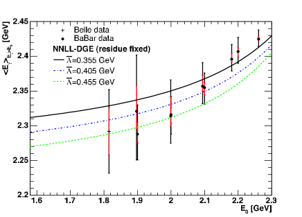
Figure 5: Comparison of experimental results from BaBar and Belle reported by Walsh $\!{}^{{\bf?}}$ to the theory of Andersen and Gardi.$\!{}^{{\bf?}}$ Here $\bar{\Lambda}$ is the difference between the $B$-meson mass and the $b$-quark mass.

4 Pentaquark states

There was some discussion at the conference of the theoretical description of the state $\Theta^{+}(1540)$, which in a quark description would be a $udud\bar{s}$ state. At the time of the conference, the experimental evidence for the existence of this state was mixed. This state is often discussed as a state consisting of two diquarks and an antiquark (see the talk of A. Vainshtein $\!{}^{{\bf?}}$ on diquarks). An alternative view, reviewed by M. Praszalowicz,$\!{}^{{\bf?}}$ derives the state in a chiral quark soliton model. This model is based on nature being near the chiral limit, in which the $\pi$ and $K$ mesons have zero mass, and near the limit of having an infinite number, $N_{c}$, of colors. Praszalowicz argued that for the $\overline{10}$ representation of flavor SU(3) to which the $\Theta^{+}(1540)$ would belong, we are far from the $N_{c}\to\infty$ limit. Thus QCD theory does not require the existence of this state. That’s good, because the existence of this state is looking more doubtful: on the day this conference ended, the COMPASS experiment reported its non-observation of the $\Theta^{+}(1540)$.$\!{}^{{\bf?}}$

5 Lattice studies

I have mentioned already lattice studies of the matrix elements for weak interaction decays. We heard two other kinds of lattice studies. One concerned the gluon propagator, the other was about one of the signals for the quark gluon plasma in heavy ion collisions.

Over the years, there have been quite a lot of studies in QCD of gluon two-point functions and three-point functions, and more generally $n$-point functions for quarks and gluons. Such studies begin with perturbation theory since they are based on the Schwinger-Dyson equations, but they go beyond any fixed order of perturbation theory by solving the equations within some approximation scheme. Since the $n$-point functions are gauge dependent, such studies must pick a gauge. F. de Soto Borrero reported on studies of the gluon two- and three-point function in QCD without dynamical quarks,$\!{}^{{\bf?}}$ based not on the Schwinger-Dyson equations but instead on a direct simulation in lattice gauge theory. One interesting way to express the results is to plot the three point function divided by the cube of the two point function, all of these suitably renormalized. That gives the one-particle-irreducible three-point function and thus an effective coupling that is a function of the momentum $p$ on each leg of the graph. I should caution that the effective coupling thus defined is a convenient object to use in discussing the theory, but is not directly observable in nature. In Fig. 6, I display the result, showing that the effective squared coupling $\alpha_{\rm MOM}$ thus defined increases as the momentum $p$ decrease, then reaches a maximum and decreases. The nice thing is that one can understand the large $p$ behavior using the operator product expansion and the small $p$ behavior using a picture involving the classical solutions of the (Euclidean) equations of motion known as instantons.

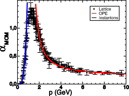
Figure 6: Effective coupling as a function of momentum, defined as $g^{2}/4\pi$ where $g$ is defined as a ratio of three and two point Green functions measured in lattice gauge theory with no dynamical quarks.$\!{}^{{\bf?}}$ The lattice results are compared to an operator product expansion expectation and to an instanton liquid model.

One signal for the quark-gluon plasma that one hopes to see in heavy ion collisions is the melting of $J/\Psi$ states. At relatively low temperatures, hadronic matter allows the existence of a $J/\Psi$ resonance. But at higher temperatures in the plasma phase, the $J/\Psi$ can no longer maintain itself. R. Petreczky presented lattice results that test this prediction. The results are shown in Fig. 7. We see that the resonance is present at low temperatures but for temperatures well above the plasma phase transition temperature $T_{c}$, it has melted away. The strength of the resonance has substantially diminished at $2.25\ T_{c}\approx 390\ {\rm MeV}$.

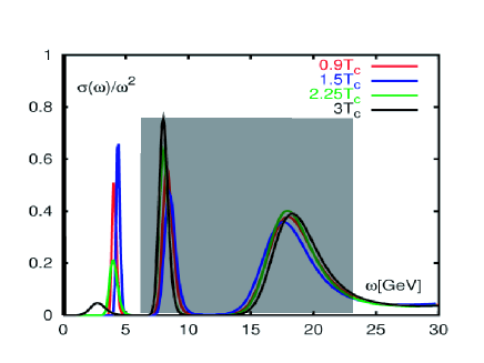
Figure 7: Spectral density in hot QCD as a function of energy $\omega$, as measured on the lattice.$\!{}^{{\bf?}}$ The data in the shaded box represents lattice artifacts and should be ignored.

6 Jet Physics

A number of talks at this conference dealt with the physics of jets. I will touch on a few topics that seemed to me to be of particular interest.

In Run I at the Fermilab Tevatron, jet cross sections were typically measured using a cone algorithm. The idea is that a jet consists of particles whose momentum vectors lie in a cone centered on a jet axis. This sounds simple. However, it is not so simple when one considers what to do with overlapping cones. For Run II, the cone algorithm has been improved with respect to sensitivity to effects from soft particles, but the complications remain. An alternative is the $k_{T}$-algorithm, which is modelled on that used in electron-positron annihilation. This algorithm is simple enough to state completely in a short paragraph. The idea is that one successively combines “nearby” subjets, thus capturing the characteristic of QCD that there are jets within jets over a wide range of transverse momentum scales. At Run II at the Tevatron, CDF and D0 have been experimenting with the use of this algorithm. A. Kupco presented data from CDF showing that the $k_{T}$-algorithm works well in a practical sense.$\!{}^{{\bf?}}$ The data is displayed in Fig. 8.

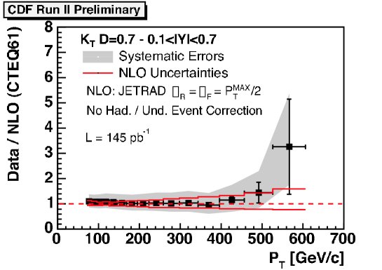
Figure 8: One jet inclusive jet cross section versus $P_{T}$ of the jet for jets defined with the $k_{T}$-algorithm,$\!{}^{{\bf?}}$ as measured by CDF. The graph shows the data divided by the NLO theory prediction, with experimental systematic errors and estimated theory errors indicated.

It has recently become possible to calculate three-jet quantities in hadron collisions at next-to-leading order. An interesting example of this is the correlation in azimuthal angle $\Delta\phi$ between two observed jets (out of three or more jets in the event). A. Kupco $\!{}^{{\bf?}}$ showed results from D0 on this quantity. The NLO theory does well in predicting the result over a wide angular range as seen in Fig. 9. (In the region close to $\Delta\phi=\pi$ we are close to the two jet region, so that fixed order perturbation is not expected to work.) The NLO theory is evidently significantly better than the LO three-jet theory, which inevitably fails as one gets near $\Delta\phi=\pi/2$ because the two jets with the largest transverse momenta cannot have $\Delta\phi=\pi/2$ unless they recoil against at least two other jets. A separate graph in this talk illustrated that the theoretical prediction from the Pythia Monte Carlo event generator is sensitive to the available tuning parameters in the $\Delta\phi\sim\pi/2$ region. Presumably Pythia would have done better if it matched to the exact tree level four-jet matrix element.

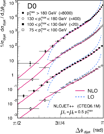
Figure 9: Two jet azimuthal angle correlation $\!{}^{{\bf?}}$ as measured by D0. The distribution is plotted against the azimuthal angle $\Delta\phi$ between the two jets for four different bins of the transverse momentum of the jet with the larger transverse momentum. For $\Delta\phi\neq\pi$ there is at least one more jet that recoils against the observed jet, so that the Born level for the theory is $\alpha_{s}^{3}$. The data is compared to LO and NLO theoretical predictions.

Jet physics took a major step forward in the 1980s with the analysis of three-jet events at the PETRA accelerator at DESY. The data is still useful, as illustrated in the talk of S. Kluth.$\!{}^{{\bf?}}$ He and collaborators used data from the Jade experiment at PETRA to extract the four jet rate at several values of $\sqrt{s}$ using the Durham (or $k_{T}$) jet algorithm. It is the progress of QCD theory that has made this difficult job worthwhile: neither the Durham algorithm nor a calculation of four jet rates at next-to-leading order were available at the time of the Jade experiment. The results provide a new way to extract $\alpha_{s}(\sqrt{s})$ from the Jade data for $\sqrt{s}$ in the PETRA energy range.

7 Perturbative calculations

In the prior sections we have seen examples of the progress in QCD theory over the years, as in the comparison of four-jet data from the Jade experiment in the early 1980s to NLO four jet calculations that have only been accomplished in the past few years. Continuing progress in theory was reported at this conference.

For a “high value” cross section like Higgs production via gluon-gluon fusion, it has been on everyone’s wish list to have a next-to-next-to-leading order calculation. Furthermore, one would like to be able to calculate the cross section for an arbitrary infrared safe observable involving the Higgs boson and other partons created in the process. This is a very difficult problem, and in my opinion the best way to do this ultimately will be to have a system of subtractions that take care of all the singularities in the partonic matrix element – based on the general singularity structure of QCD. However, progress in this direction has been slow. C. Anastasiou discussed a program that does just this task based not on knowing the singularity structure of QCD but on letting a computer find the singularities.$\!{}^{{\bf?}}$ For three final state partons, one maps the momenta $\{p_{1},p_{2},p_{3}\}$ constrained to have the sum of the transverse momenta vanish into seven variables $\{x_{1},x_{2},x_{3},x_{4},x_{5},x_{6},x_{7}\}$ in a seven dimensional hypercube. The mapping should be such that the singularities are at the edges and faces of the hypercube. Then the computer is asked to find the singularities and make the appropriate subtractions. I can illustrate the idea in a simple fashion if I use only two variables $x$. Consider an integral of the form

$$I=\int_{0}^{1}dx_{1}\,x_{1}^{\epsilon}\int_{0}^{1}dx_{2}\,\frac{f(x_{1},x_{2})}{x_{1}},$$ (2)

where the factor $x_{1}^{\epsilon}$ mimics the result of using dimensional regularization and $f(x_{1},x_{2})$ is a smooth function that could be quite complicated. We would like to separate this into a pole term proportional to $1/\epsilon$ and a term that is finite as $\epsilon\to 0$. To this end, we ask our computer to notice the singularity at $x_{1}\to 0$ and write the integral as

$$\begin{split}I={}&\int_{0}^{1}dx_{1}\,x_{1}^{\epsilon}\int_{0}^{1}dx_{2}\left\{\frac{f(0,x_{2})}{x_{1}}+\frac{f(x_{1},x_{2})-f(0,x_{2})}{x_{1}}\right\}\\ \sim{}&{\frac{1}{\epsilon}}\int_{0}^{1}dx_{2}\,f(0,x_{2})+\int_{0}^{1}dx_{1}\int_{0}^{1}dx_{2}\ \frac{f(x_{1},x_{2})-f(0,x_{2})}{x_{1}}.\end{split}$$ (3)

The first term is the pole term, the second is the finite term. Both integrals can be computed by numerical integration. In real life, the situation is much more complicated, but it appears from the results presented in $\!{}^{{\bf?}}$ that this is a practical way to proceed.

By going from NLO calculations to NNLO calculations, one reduces the estimated theory error for the prediction of a certain class of cross sections. There is also another needed direction for improvement of calculations.

Conventional NLO calculations do not do well at predicting the probability to emit soft particles or at describing the inner structure of jets. That is why one restricts their use to the prediction of those cross sections that are “infrared safe” in the sense that they are not sensitive to soft particles in the final state or to how jets are divided into subjets. For instance, suppose that one were to take a program that gives the cross section for $p+\bar{p}\to W+{\it jet}+X$ at NLO. Now imagine using the program to predict the distribution of masses for the jet. The result would be a certain number of events with jet masses near 10 GeV, more events with jet masses near 5 GeV, many more with jet masses near 1 GeV, and yet more with yet smaller jet masses. This all adds up to an infinite number of events, but the situation is saved by having an infinitely negative number of events with jet mass zero. Evidently, this is not a satisfactory description of nature. Nor is it satisfactory that the jets are made of one or two partons rather than many hadrons.

Clearly it would be better to let the partons fragment to form parton showers and then let the parton showers form hadrons in the style of event generator Monte Carlo programs like Pythia and Herwig. It is, however, not so easy to do this while maintaining the next-to-leading order accuracy of the calculation for the infrared safe quantities that the NLO program was designed to get right.

There has been some progress in this area in recent years,$\!{}^{{\bf?}}$ but the presently existing programs are either tied to a specific Monte Carlo event generator or a limited class of processes and are not specified in a simple general algorithm that authors of NLO calculations could easily use.

At this conference, Z. Nagy $\!{}^{{\bf?}}$ presented an algorithm for extending an NLO calculation in a fashion that would allow partonic events from the modified NLO program to be fed to a Monte Carlo event generator for showering and hadronization, on the condition that the showering be started for each event with suitable initial conditions. The algorithm is presented for jet production in electron-positron annihilation, but it should be possible to extend it to lepton-hadron and hadron-hadron collisions. The idea is to base the algorithm on the Catani-Seymour dipole subtraction scheme $\!{}^{{\bf?}}$ that is widely used in constructing NLO programs. In addition, the algorithm makes use of the $k_{T}$ jet-matching scheme $\!{}^{{\bf?}}$ for switching descriptions among, for example, $p+\bar{p}\to W+X$, $p+\bar{p}\to W+1\ {\it jet}+X$, and $p+\bar{p}\to W+2\ {\it jets}+X$. This is so far an algorithm but not yet code. Perhaps we will see a working program at the XLI Rencontre de Moriond.

8 QCD in the high energy/small $x$ limit

At this conference there was quite a lot of discussion of how QCD behaves when seen with experiments that, in one view, probe the gluon distribution at small momentum fraction $x$. Relevant experiments include deeply inelastic scattering at small Bjorken $x$ and heavy ion collisions at RHIC.

An outsider like me can understand at least part of this discussion with the aid of a few of simple observations. First, the whole subject hinges on how systems with vastly different rapidities can interact. For instance, if one is interested in the total cross section for scattering two nuclei at high energy, the rapidity difference $\Delta y=\log(s/M^{2})$ is large. In deeply inelastic scattering, the rapidity difference between the virtual photon and the proton is $\Delta y=\log(Q/m)+\log(1/x)$ and is large if $x$ is small (even if $Q/m$ is not so large). Second, systems with a large rapidity difference can communicate easily by exchanging gluons, so that the whole subject hinges on gluons. Third, experiment shows that lots of gluons are to be found in the proton carrying a small fraction $x$ of the proton’s momentum. Thus the small $x$ gluons appear to be densely packed inside the transverse size of a proton or nucleus. With respect to a probe that might measure this gluon distribution by scattering from it, the hadron looks black. This suggests a system that is purely non-perturbative and thus resistant to theoretical analysis. However, it is useful to think of our probe as a fast moving color dipole. For instance, in deeply inelastic scattering, the virtual photon creates a quark-antiquark pair with net color zero – that is a color dipole. This leads to the fifth observation: If the dipole is small enough, the dense gluonic system is transparent to the dipole. Thus there is some size $1/Q_{s}(x)$ for which the gluonic system just starts to scatter the dipole. At small $x$, the density of gluons is so high $1/Q_{s}(x)$ is small. That is, the “saturation scale” $Q_{s}(x)$ is big. This means that there is naturally a big transverse momentum scale in the problem and perturbation theory can be helpful. This analysis does not carry us very far into the subtleties of the theory, but it is perhaps useful in getting us started.

One approach to the high energy limit of QCD is the much studied BFKL equation. There is a leading order version of this equation and, more recently, next-to-leading order corrections. However, it has appeared that the general approach is unstable, with the corrections leading to big changes in the behavior of the solutions. At this conference, L. Schoeffel $\!{}^{{\bf?}}$ discussed ways of modifying the equation so as to avoid some of the problems and showed results for the solutions of the resulting equation. J. Andersen $\!{}^{{\bf?}}$ took a different approach, arguing that the widely used Mellin transform method of solving the BFKL equation leads to problems, so that one should instead use an iterative numerical approach. If one defines an effective pomeron intercept $\alpha_{I\kern-5.0ptP}$ by $xg(x)\sim x^{-\alpha_{I\kern-5.0ptP}}$, then Andersen finds a sensible behavior for $\alpha_{I\kern-5.0ptP}$ as a function of rapidity, as shown in Fig.!10.

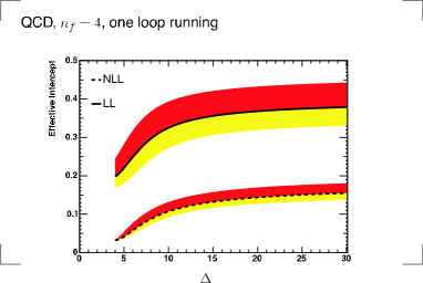
Figure 10: Behavior of the effective pomeron intercept according to the BFKL equation as a function of rapidity $\Delta$ from the talk of J. Andersen.$\!{}^{{\bf?}}$ Solutions are shown for the lowest order equation and for the next-to-leading order equation solved by an iterative numerical method. Note that the effective intercept at next-to-leading order is fairly small and approximately constant as $\Delta$ increases.

Another approach to understanding the high energy limit of QCD is to go beyond the BFKL equation. There were separate talks on this by E. Iancu,$\!{}^{{\bf?}}$ by D. Triantafyllopoulos $\!{}^{{\bf?}}$ and by G. Soyez.$\!{}^{{\bf?}}$ Here, I follow mostly Iancu and Triantafyllopoulos. One considers the interaction of a color dipole with a hadron to be created by the exchange of $n$ gluon ladders, or “pomerons.” Letting $T_{n}$ be contribution from for $n$ pomerons, one writes an equation for the variation of $T_{n}$ with the rapidity $y$ of the dipole relative to the hadron,

$$dT_{n}/dy=K_{\rm BFKL}\,T_{n}+K_{\rm split}\,T_{n-1}+K_{\rm merge}\,T_{n+1}\ .$$ (4)

Here the $T_{n}$ are functions of transverse position arguments and the various $K$ are kernels in an integral equation. This general scheme incorporates the linear evolution of a gluon ladder, the splitting of one ladder to make two, and the joining of two gluon ladders to make one. The first term, for $n=1$ is the leading order BFKL equation. Triantafyllopoulos argued that the splitting and merging terms are more important than the next-to-leading order corrections to the BFKL equation. Iancu argued that one has some hope of making progress with the splitting-joining picture, even though it is complicated, since the problems are related to problems that have been studied in statistical physics.

9 Automating the scientific method

Part of the purpose of this talk was to provide some assessment of where we stand with respect to the problems and opportunities facing QCD theory. Of particular interest is the upcoming beginning of the LHC era. One anticipates that what is seen may not be in agreement with the Standard Model. Since the incoming particles and many of the outgoing particles in an LHC event carry the strong interactions, one is going to have to incorporate QCD theory into the interpretation of whatever signals may be found. Are we ready?

B. Knutsen $\!{}^{{\bf?}}$ presented computer tools that can help in the interpretation of the data. First, there are tools for finding discrepancies between the data and Standard Model predictions. Then, there are tools for testing hypotheses against the data. Finally, there is a tool for generating hypotheses and testing them. One might call this last step automating theorists.

I am a bit skeptical about this last part. Of course, it is not the theorists who construct computer programs for doing calculations who are in danger of being replaced by automatons: their programs would just be added to the array of programs that does hypothesis testing. Rather, it is the model building theorists whom we perhaps don’t need. However, my guess is that we will be faced with a more difficult problem than simply filling in the blanks for the Minimal Supersymmetric Standard Model, so that some clever ideas from people like those who built the MSSM will be required.

Overall, it seems to me that we ought to automate whatever we can. However, I was struck by Knutsen’s comment that high energy physics is behind astrophysics, heavy ion physics, and biology with respect to automation. Accordingly, I would like to present a real example from current developmental biology that provides an interesting comparison to high energy physics.

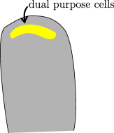
Figure 11: Sketch of region dual purpose cells in a zebrafish embryo.

The example concerns the zebrafish, a small tropical fish that is easily raised in tanks. This fish has the wonderful feature that its embryos are quite transparent, so that the parts of an embryo can be studied under a microscope as the embryo develops. Study of how the embryo develops can help us figure out the mechanisms for development. One finds $\!{}^{{\bf?}}$ that in the early embryo there is a band of cells that are able to be either pituitary gland cells or else cells in the lens of the fish’s eye (Fig. 11). How, then, do these cells decide what to do? Experiments $\!{}^{{\bf?}}$ show that there are some nearby cells that express a signalling molecule called Hedgehog. The dual purpose cells that get a strong Hedgehog signal become pituitary gland cells, while those that get a weaker signal become lens cells (Fig. 12). One can test this by using a mutant fish that does not produce Hedgehog. This amounts to changing the DNA of the starting fish egg.

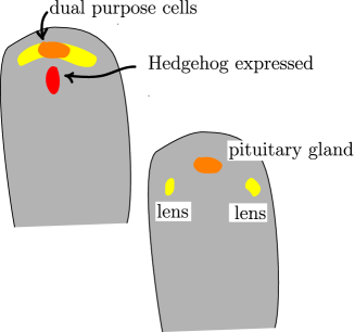
Figure 12: Sketch illustrating the role of Hedgehog signalling protein in determining the fate of the dual purpose cells in Fig. 11.

The experiments in biology that lead to such discoveries are difficult. Things would be easier if biologists could automate the process by producing a computer program, which might be called Icthia, that could simulate fish development (Fig. 13). The input would be the fish genome. Then the program would simulate the complete development of the fish, including the signalling pathways just discussed. In the end, we would have a model final state fish to compare to an experimental fish.

Of course, there is no such program. Biology is too hard for that. But physics is easier. We do have programs, for instance Pythia, that take the lagrangian of the Standard Model or various extensions as input and simulate the entire development of high energy physics events, from an initial state shower to a hard interaction such as, say, a quark and antiquark producing a squark and antisquark, followed by parton showering and decays, followed by hadronization, producing final states of events that can be compared to experimental events (Fig. 14).

We thus have, I submit, theoretical tools for the analysis of the upcoming LHC experiments that are extraordinarily powerful. The event generator Monte Carlo programs just described have a very wide scope. There are also well automated tools for creating tree level cross sections for an even wider variety of partonic processes. Where more accuracy is needed for suitably inclusive cross sections, we have NLO programs and even some NNLO programs. These tools have been developed over the last couple of decades and are now, I think, adequate to the task at hand. Furthermore, these theory tools are currently being improved. It was a pleasure to hear about some of the progress at this conference. The more improvements we have, the better off we will be in trying to understand what we find at the LHC.

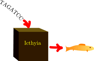
Figure 13: How to automate developmental biology. Build a computer program that takes a DNA sequence as input and models the development of a fish.

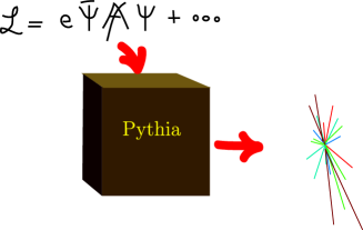
Figure 14: How particle physics has already been automated. Pythia takes the lagrangian as input and models the development of $pp$ collision events. Herwig does this too. (Of course, there are limitations, for instance with respect to the range of input lagrangians that are programmed and with respect to the accuracy of the output.)

References

References

- [1] I. Belyaev, these proceedings. Similar data may be found in F. Abe et al. [CDF Collaboration] Phys. Rev. Lett. 75 (1995) 1451.
- [2] M. d’Onofrio, these proceedings.
- [3] T. Huber, these proceedings.
- [4] S. Schilling, these proceedings.
- [5] M. Okamoto, these proceedings.
- [6] E. Gardi, these proceedings.
- [7] J. Walsh, these proceedings.
- [8] E. Gardi and J. Andersen, private communication, this conference.
- [9] A. Vainshtein, these proceedings.
- [10] M. Praszalowicz, these proceedings.
- [11] E. S. Ageev et al,. [COMPASS Collaboration], arXiv:hep-ex/0503033.
- [12] F. de Soto Borrero, these proceedings.
- [13] R. Petreczky, these proceedings.
- [14] A. Kupco, these proceedings.
- [15] S. Kluth, these proceedings.
- [16] C. Anastasiou, these proceedings.
- [17] S. Frixione and B. R. Webber, JHEP 0206, 029 (2002); S. Frixione, P. Nason and B. R. Webber, JHEP 0308, 007 (2003); M. Krämer and D. E. Soper, Phys. Rev. D 69, 054019 (2004); D. E. Soper, Phys. Rev. D 69, 054020 (2004).
- [18] Z. Nagy, these proceedings
- [19] S. Catani and M. H. Seymour, Nucl. Phys. B 485 (1997) 291 [Erratum-ibid. B 510 (1997) 503].
- [20] S. Catani, F. Krauss, R. Kuhn and B. R. Webber, JHEP 0111 (2001) 063.
- [21] L. Schoeffel, these proceedings.
- [22] J. Andersen, these proceedings.
- [23] E. Iancu, these proceedings.
- [24] D. Triantafyllopoulos, these proceedings.
- [25] G. Soyez, these proceedings.
- [26] B. Knutsen, these proceedings.
- [27] S. Dutta et al., Development et al. 132 (2005) 1579.