Oscillations of high energy neutrinos in matter: Precise formalism
and parametric resonance

Abstract

We present a formalism for precise description of oscillation phenomena in matter at high energies or high densities, $V>\Delta m^{2}/2E$, where $V$ is the matter-induced potential of neutrinos. The accuracy of the approximation is determined by the quantity $\sin^{2}2\theta_{m}\Delta V/2\pi V$, where $\theta_{m}$ is the mixing angle in matter and $\Delta V$ is a typical change of the potential over the oscillation length ($l\sim 2\pi/V$). We derive simple and physically transparent formulas for the oscillation probabilities, which are valid for arbitrary matter density profiles. They can be applied to oscillations of high energy ($E>10$ GeV) accelerator, atmospheric and cosmic neutrinos in the matter of the Earth, substantially simplifying numerical calculations and providing an insight into the physics of neutrino oscillations in matter. The effect of parametric enhancement of the oscillations of high energy neutrinos is considered. Future high statistics experiments can provide an unambiguous evidence for this effect.

1. Introduction. Neutrino physics enters a new phase now, where the objectives are precision measurements of the parameters, studies of subleading oscillation effects and searches for new physics beyond the already standard picture, which includes non-zero neutrino masses and mixing. Detection of neutrinos from new sources, in particular, of cosmic neutrinos, is in the agenda.

Substantial new information is expected from the studies of high energy ($E>1$ GeV) neutrinos. This includes investigations of atmospheric neutrinos with new large volume detectors fatm , long baseline accelerator experiments LBL and detection of cosmic neutrinos from galactic and extragalactic sources, as well as of neutrinos produced in interactions of cosmic rays with the solar atmosphere solatm . Another possible source of neutrinos is annihilation of hypothetical WIMP’s in the center of the Earth and the Sun WIMPS . In all these cases beams of high energy neutrinos can propagate significant distances in the matter of the Earth (or of the Sun) and therefore undergo oscillations/conversions in matter.

Increased accuracy and reach of neutrino experiments put forward new and more challenging demands to the theoretical description of neutrino oscillations. In the present Letter we derive very simple and accurate analytic formulas describing oscillations of neutrinos in matter. Our primary goal is to study oscillations of high energy neutrinos note1 , but the formulas we obtain are actually applicable in a wide range of neutrino energies. They simplify substantially numerical calculations and allow a deep insight into the physics of neutrino conversions in matter. In particular, they provide a useful tool for studying parametric resonance enhancement of neutrino oscillations.

The parametric resonance can occur in oscillating systems with varying parameters due to a specific correlation between the rate of the change of these parameters and the values of the parameters themselves. In the case of neutrino oscillations in matter, the parametric enhancement is realized when the variation of the matter density along the neutrino trajectory is in a certain way correlated with the change of the oscillation phase ETC ; Akh1 . This effect is different from the MSW effect W ; MS , and yet can result in a strong amplification of the oscillations. We apply the formalism developed here to study the parametric resonance in oscillations of high energy neutrinos in the Earth.

2. Formalism. We consider oscillations in the 3-flavor neutrino system ($\nu_{e},\,\nu_{\mu},\,\nu_{\tau}$), with the mass squared differences $\Delta m_{31}^{2}$ and $\Delta m_{21}^{2}$ responsible for the oscillations of atmospheric and solar neutrinos, respectively. In certain situations, the full three-flavor problem is approximately reduced to the effective two-flavor ones, in which the electron neutrino $\nu_{e}$ oscillates into a combination of $\nu_{\mu}$ and $\nu_{\tau}$. We shall be mainly interested in oscillations of neutrinos with energies $E>\Delta m_{31}^{2}/2V$, where the matter-induced potential of neutrinos $V(x)\equiv\sqrt{2}G_{F}N_{e}(x)$, with $N_{e}(x)$ the electron number density in matter and $G_{F}$ the Fermi constant. Numerically, this corresponds to $E>8-10$ GeV for the matter of the Earth. In this case the 1-2 mixing is strongly suppressed by matter, and the problem is reduced to an effective two-flavor one, described by the potential $V$, mass squared difference $\Delta m^{2}\equiv\Delta m_{31}^{2}$ and vacuum mixing angle $\theta\equiv\theta_{13}$ (which is assumed to be non-zero) ADLS . In particular, the oscillations of electron neutrinos are determined by the transition probability $P_{2}\equiv P(\nu_{e}\leftrightarrow\nu_{a})$, where $\nu_{a}=\sin\theta_{23}\nu_{\mu}+\cos\theta_{23}\nu_{\tau}$ is the state which mixes with $\nu_{e}$ in the third mass eigenstate. In terms of $P_{2}$ the flavor transition probabilities are $P(\nu_{e}\rightarrow\nu_{\mu})=P(\nu_{\mu}\rightarrow\nu_{e})=\sin^{2}\theta_{23}P_{2}$, $P(\nu_{e}\rightarrow\nu_{\tau})=P(\nu_{\tau}\rightarrow\nu_{e})=\cos^{2}\theta_{23}P_{2}$ ADLS . The third state (orthogonal to $\nu_{a}$) decouples from the rest of the system and evolves independently.

In the ($\nu_{e},\,\nu_{a})$ basis, the evolution matrix $S(x)$ describing neutrino oscillations satisfies the equation

$$i\frac{dS}{dx}=H(x)S\,,$$ (1)

with the Hamiltonian

$$H(x)=\frac{V}{2}\left(\!\!\begin{array}[]{cc}~{}1&~{}~{}0{}\\ ~{}0&-1\end{array}\!\!\right)+\delta\left(\!\!\begin{array}[]{cc}-\cos 2\theta&~{}\sin 2\theta\\ ~{}\sin 2\theta&~{}\cos 2\theta\end{array}\!\!\right).$$ (2)

Here

$$\delta\equiv\Delta m^{2}/4E\,,$$ (3)

and the first (potential) term dominates in the high energy limit. However, in most situations of interest the neutrino path length in matter $L$ satisfies $\delta\cdot L\gtrsim 1$, therefore we cannot consider the whole second term as a small perturbation, and the effect of $\delta$ on the neutrino energy level splitting should be taken into account. For this reason we split the Hamiltonian as

$$H=H_{0}+H_{I},$$ (4)

with

$$H_{0}=\omega\left(\!\!\begin{array}[]{cc}~{}1&~{}~{}0{}\\ ~{}0&-1\end{array}\!\!\right),~{}~{}~{}H_{I}=\sin 2\theta\,\delta\,\left(\!\!\begin{array}[]{cc}-\epsilon&~{}1\\ ~{}1&~{}\epsilon\end{array}\!\!\right)\,.$$ (5)

Here

$$\omega(x)\equiv\sqrt{(V/2-\delta\cos 2\theta)^{2}+\delta^{2}\sin^{2}2\theta}\,,$$ (6)

$2\omega$ being the difference of the eigenvalues of $H(x)$;

$$\epsilon\equiv\frac{\cos 2\theta\,\delta-V/2+\omega}{\sin 2\theta\,\delta}\approx\frac{\delta}{V}\sin 2\theta\ll 1.$$ (7)

The ratio of the second and the first terms in the Hamiltonian in (5) is determined by the mixing angle in matter $\theta_{m}$:

$$\frac{\sin 2\theta\,\delta}{\omega}=\sin 2\theta_{m}\,.$$ (8)

Therefore for $\sin 2\theta_{m}\ll 1$ the term $H_{I}$ can be considered as a perturbation. Furthermore, according to (7), $\epsilon\sim\sin 2\theta_{m}$, so that the diagonal terms in $H_{I}$ can be neglected in the lowest approximation.

We seek the solution of eq. (1) in the form

$$S=S_{0}\cdot S_{I}\,,$$ (9)

where $S_{0}$ is the solution of the evolution equation with $H$ replaced by $H_{0}$. From (5) we find

$$S_{0}(x)=\left(\begin{array}[]{cc}e^{-i\phi(x)}{}&0{}\\ 0&e^{i\phi(x)}{}\end{array}\right),$$ (10)

where

$$\phi(x)\equiv\int_{0}^{x}dx^{\prime}\,\omega(x^{\prime})$$ (11)

is the adiabatic phase. Then, according to (1), (4) and (9), the matrix $S_{I}$ satisfies the equation

$$i\frac{dS_{I}}{dx}=S_{0}^{-1}H_{I}S_{0}\,S_{I}=\tilde{H}_{I}S_{I}\,,$$ (12)

where $\tilde{H}_{I}\equiv S_{0}^{-1}H_{I}S_{0}$ is the perturbation Hamiltonian in the “interaction” representation. Eq. (12) can be solved by iterations: $S_{I}=\mathbbm{1}+S_{I}^{(1)}+...$, which leads to the standard perturbation series for the $S$ matrix. For neutrino propagation between $x=0$ and $x=L$ we have

$$S_{I}(L)=\mathbbm{1}-i\int_{0}^{L}dx\tilde{H}_{I}(x)-\int_{0}^{L}dx\tilde{H}_{I}(x)\int_{0}^{x}dx^{\prime}\tilde{H}_{I}(x^{\prime})...$$ (13)

Taking $S_{I}$ to the first order, we obtain from (9) the evolution matrix

$$S(L)=S_{0}(L)\left[\mathbbm{1}-i\delta\sin 2\theta\int_{0}^{L}dx\left(\begin{array}[]{cc}0&e^{i2\phi(x)}{}\\ e^{-i2\phi(x)}&0{}\end{array}\right)\right].$$ (14)

The $\nu_{e}\leftrightarrow\nu_{a}$ transition probability $P_{2}(L)$ is given by the squared modulus of the off-diagonal element $[S(L)]_{ae}$:

$$P_{2}=\delta^{2}\sin^{2}2\theta\left|\int_{0}^{L}dx~{}e^{-i2\phi(x)}\right|^{2}.$$ (15)

For density profiles that are symmetric with respect to the center of the neutrino trajectory, $V(x)=V(L-x)$, eq. (15) gives

$$P_{2}=4\left(\frac{\Delta m^{2}}{4E}\right)^{2}\sin^{2}2\theta\left[\int_{0}^{L/2}dz\cos 2\phi(z)\right]^{2},$$ (16)

where $z=x-L/2$ is the distance from the midpoint of the trajectory and $\phi(z)$ is the phase acquired between this midpoint and the point $z$.

The transition probability $P_{2}$ scales with neutrino energy essentially as $E^{-2}$. The accuracy of eq. (15) also improves with energy as $E^{-2}$. This is illustrated by panels (a) and (b) of fig. 1, which show $P_{2}$ as a function of neutrino energy for several trajectories inside the Earth and as a function of the zenith angle of the neutrino trajectory $\Theta$ for several neutrino energies. One can see that already for $E\gtrsim 8$ MeV the accuracy of our analytic formula is extremely good. Note that when neutrinos do not cross the Earth’s core ($\cos\Theta>-0.837$) and so experience a slowly changing potential $V(x)$, the accuracy of the approximation (15) is very good even in the MSW resonance region $E\sim$5 – 8 GeV. The accuracy of eq. (15) is also good for energies below $\sim 2$ GeV (not shown in the figure); however, in this region the domain of the applicability of (15) is relatively narrow, since for $E\lesssim 0.5$ GeV the oscillations driven by the “solar” parameters ($\Delta m_{21}^{2},\,\theta_{12}$) can no longer be neglected.

To understand the remarkable accuracy of eq. (15), we find the correction $\Delta P_{2}$ to the transition probability in (15) emerging in the next nontrivial order in $H_{I}$. Note that from the above considerations one can expect $\Delta P_{2}/P_{2}$ to be proportional to $\sin 2\theta_{m}$. Furthermore, as can be easily seen, for uniform matter eq. (15) reproduces the exact transition probability; therefore one expects $\Delta P_{2}/P_{2}\propto V^{\prime}$. A straightforward calculation indeed gives

$$\frac{\Delta P_{2}}{P_{2}}\simeq\sin^{2}2\theta_{m}\,\frac{\Delta V}{4\pi\omega}\simeq\sin^{2}2\theta_{m}\,\frac{\Delta V}{2\pi V}\,,$$ (17)

where $\Delta V$ is the change of the potential over the oscillation length $\pi/\omega$, and the last equality holds in the high energy regime. For slowly changing density this is equivalent to

$$\frac{\Delta P_{2}}{P_{2}}\simeq\sin^{2}2\theta_{m}\,\frac{V^{\prime}}{4\omega^{2}}\,.$$ (18)

Introducing the adiabaticity parameter $\gamma=4\pi\omega/(\sin 2\theta_{m}\Delta V)$, we find that $\Delta P_{2}/P_{2}\simeq\sin 2\theta_{m}\gamma^{-1}$, and therefore for small mixing in matter our approximation is better than the adiabatic one. At the same time, for $\Delta V/4\pi\omega<1$ it is better than the simple expansion in powers of $\sin^{2}2\theta_{m}$.

The matter density profile of the Earth satisfies $V^{\prime}/V^{2}\lesssim 0.5$, and therefore for neutrino oscillations in the Earth our approximation is expected to work well when $\sin^{2}2\theta_{m}\ll 1$. This is fulfilled in the high energy (or, equivalently, high density) limit $EV/\Delta m^{2}\gg\cos 2\theta$, i.e. above the MSW resonance. If the vacuum mixing angle is small (i.e. $\theta=\theta_{13}$), our expansion parameter is also small below the resonance. The above formalism applies in this low energy case as well, with only minor modifications: the sign of $H_{0}$ in (5) has to be flipped, and correspondingly one has to replace $\omega\to-\omega$ in eq. (7). These modifications are necessary because of the interchange of the eigenvalues of the Hamiltonian upon crossing the MSW resonance. Expressions for the transition probability in eqs. (15), (16) remain unchanged. Thus, our results are in general valid outside the MSW resonance region, which for small $\theta$ is very narrow. For the non-resonant channels ($\bar{\nu}$ channels for $\Delta m^{2}>0$ or $\nu$ channels for $\Delta m^{2}<0$) and small vacuum mixing our formulas are valid in the whole diapason of energies because $\sin 2\theta_{m}$ is always small.

If $\theta_{13}$ is very small or vanishes, $\nu_{e}\leftrightarrow\nu_{\mu,\tau}$ oscillations are driven by $\Delta m^{2}=\Delta m_{21}^{2}$ and the large mixing angle $\theta=\theta_{12}$. The oscillation probabilities can then be expressed through another effective two-flavor probability, $\tilde{P}_{2}\equiv\tilde{P}_{2}(\Delta m_{21}^{2},\,\theta_{12},\,V(x))$, in terms of which the flavor transition probabilities are $P(\nu_{e}\leftrightarrow\nu_{\mu})=\cos^{2}\theta_{23}\tilde{P}_{2}$, $P(\nu_{e}\leftrightarrow\nu_{\tau})=\sin^{2}\theta_{23}\tilde{P}_{2}$ PerSm . For $EV/\Delta m_{21}^{2}\gg\cos 2\theta_{12}$ (which for the typical densities inside the Earth corresponds to $E\gtrsim 0.5$ GeV), the probability $\tilde{P}_{2}$ is very well approximated by eq. (15).

Let us consider the case of symmetric matter. Integrating (16) by parts, one finds

$$P_{2}=\sin^{2}2\theta_{m}^{0}\left[\sin\phi_{L}+\omega_{0}\int^{L/2}_{0}dz\frac{d\omega}{dz}\frac{1}{\omega^{2}}\sin 2\phi(z)\right]^{2}\,,$$ (19)

where $\theta_{m}^{0}\equiv\theta_{m}(V_{0})$, $\omega_{0}\equiv\omega(V_{0})$, $V_{0}$ being the potential at the initial and final points of the neutrino trajectory, and $\phi_{L}$ is the adiabatic phase acquired along the entire neutrino path. If the potential changes slowly with distance, so that $\omega^{-2}d\omega/dz\ll 1$, the second term in (19) can be neglected, and $P_{2}$ reduces to the usual adiabatic probability in symmetric matter: $P_{\rm adiab}=\sin^{2}2\theta_{m}^{0}\sin^{2}\phi_{L}$. The second term in (19) describes the effects of violation of adiabaticity.

Let us apply the above results to neutrino beams (atmospheric, accelerator, cosmic neutrinos) crossing the Earth. According to the PREM model PREM , the Earth density profile can be described as several spherical shells of radii $R_{i}$ with rather smooth density change within the shells and sharp change at the borders between them. Then, along a direction from the center of the Earth outwards, $\omega(z)$ decreases abruptly from $\omega_{i}^{+}$ to $\omega_{i}^{-}$ in very narrow regions around $R_{i}$. Therefore $d\omega/dz$ is large in these narrow regions and small outside them. The integration in (19) can then be easily done, leading to

$$P_{2}=\sin^{2}2\theta_{m}^{0}\left[\sin\phi_{L}-\omega_{0}\Sigma_{i}\frac{\omega_{i}^{+}-\omega_{i}^{-}}{\omega_{i}^{+}\omega_{i}^{-}}\sin 2\phi_{i}\right]^{2}.$$ (20)

Here $\phi_{i}$ is the adiabatic phase acquired by neutrinos between the points $z=0$ and $z=R_{i}$. We will use eq. (20) for interpreting the results of our calculations.

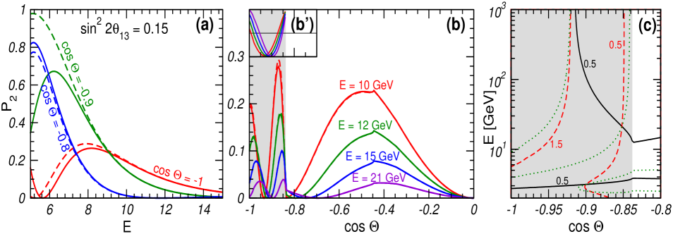
Figure 1: Panels (a) and (b): transition probability $P_{2}$ vs neutrino energy for different trajectories inside the Earth [panel (a)] and vs $\cos\Theta$ for different neutrino energies [panel (b)]. Solid curves are the results of exact numerical calculations, dashed curves are obtained using formula (15). Small window (b’) in panel (b) shows the values of the parameter $X_{3}$ [eq. (25)] calculated in the three-layer model of the Earth’s density. Panel (c): contours of constant phases $\phi_{m}$ (solid curves), $\phi_{c}$ (dashed curves) and of constant $X_{3}=0$ (dotted curves). The numbers at the curves are the values of the phases in units of $\pi$. The shaded areas in panesls (b) and (c) correspond to the Earth’s core. For all panels we take $\sin^{2}2\theta_{13}=0.15$ and $\Delta m^{2}=2\cdot 10^{-3}$ eV².

3. Parametric enhancement of oscillations. In the PREM model of the Earth density all the density jumps between different shells except those between the mantle and core are relatively small PREM . Therefore the density profile felt by neutrinos crossing the core of the Earth can be approximated by three layers (mantle - core - mantle) with slow density changes within the layers. Eq. (20) then gives

$$P_{2}=\sin^{2}2\theta_{m}^{0}\left[\sin(\phi_{c}+2\phi_{m})-\frac{\omega_{0}}{\omega_{m}}\left(1-\frac{\omega_{m}}{\omega_{c}}\right)\sin\phi_{c}\right]^{2},$$ (21)

where $\omega_{m}$ and $\omega_{c}$ are the values of $\omega(x)$ in the mantle and core on the respective sides of their border, and $\phi_{m}$ and $\phi_{c}$ are the phases acquired in the mantle (one layer) and core. Eq. (21) corresponds to the adiabatic neutrino propagation inside the core and mantle and violation of the adiabaticity at the borders between them. In the approximation of constant effective densities in the mantle and core we have $\omega_{0}=\omega_{m}^{\rm eff}$, and the non-adiabatic term is proportional to $(1-\omega_{c}^{\rm eff}/\omega_{m}^{\rm eff})$.

For neutrino trajectories that cross the mantle only ($\phi_{c}=0$), eq. (21) reduces to the adiabatic probability. The passage of neutrinos through the core can lead to an enhancement of the oscillations. As follows from (21), the maximum enhancement of the probability can be achieved when $\sin(\phi_{c}+2\phi_{m})$ and $\sin\phi_{c}$ are of opposite sign and maximal amplitude:

$$\sin\phi_{c}=-\sin(\phi_{c}+2\phi_{m})=\pm 1,$$ (22)

that is, when

$$\phi_{c}=\pm\frac{\pi}{2}+2\pi n,~{}~{}~{}\phi_{m}=\pm\frac{\pi}{2}+2\pi k\,.$$ (23)

Here $n$ and $k$ are integers, and the signs in front of $\pi/2$ are correlated. In this case the enhancement factor is

$$\frac{P_{2}^{max}}{\sin^{2}2\theta_{m}}=\left[1+\frac{\omega_{0}}{\omega_{m}}\left(1-\frac{\omega_{m}}{\omega_{c}}\right)\right]^{2}\approx\left(2-\frac{V_{m}}{V_{c}}\right)^{2}\approx 2.5\,,$$ (24)

where $\sin^{2}2\theta_{m}$ in the denominator corresponds to the maximum possible transition probability for neutrinos crossing only the mantle, and we have taken into account that at high energies $\omega_{m}/\omega_{c}\approx V_{m}/V_{c}$.

The condition in eq. (23) and the enhancement described by eq. (24) are the particular cases of the parametric resonance condition and the parametric enhancement of neutrino oscillations ETC ; Akh1 . In Akh2 it was shown that in the case of matter consisting of alternating layers of two different constant densities and (in general) different widths the parametric resonance condition is

$$X_{3}\equiv-(\sin\phi_{m}\cos\phi_{c}\cos 2\theta_{m}+\cos\phi_{m}\sin\phi_{c}\cos 2\theta_{c})=0\,,$$ (25)

where $\theta_{m,c}$ and $\phi_{m,c}$ are the mixing angles and the acquired oscillations phases in the layers $m$ and $c$. This condition can also be used as an approximate one when matter density inside the layers is not constant but varies sufficiently slowly. For neutrino oscillations in the Earth we identify the layers $m$ and $c$ with the mantle and core. Since in the energy region $\sin 2\theta\,\delta\ll V$ one has $\theta_{m}\approx\theta_{c}\approx\pi/2$, condition (25) reduces to

$$X_{3}\simeq\sin(\phi_{m}+\phi_{c})=0\,.$$ (26)

Eq. (23) is a particular realization of this condition. In the high energy limit the parametric resonance condition (23) was previously considered in the framework of active-sterile atmospheric neutrino oscillations in Liu . It should be noted that, while the realization (23) of condition (25) corresponds to the maximal possible parametric enhancement of oscillations of high energy neutrinos in the Earth, a sizable amplification is also possible if the equality $X_{3}=0$ is realized differently, i.e. when the two terms in (25) do not separately vanish but cancel each other note2 .

The parametric resonance conditions in eq. (25) or (23) require a subtle correlation between the matter density of the Earth, the distances that neutrinos travel in the Earth’s mantle and core (which are not independent), and also in general neutrino energy and oscillation parameters. Therefore it is far from obvious that these conditions can actually be satisfied. Amazingly, this is indeed the case Liu ,Pet ,Akh2 .

Our present analysis shows that, for $\nu_{e}\leftrightarrow\nu_{\mu,\tau}$ oscillations of high energy neutrinos in the Earth, there are two regions of the zenith angles of neutrino trajectories in which (25) is satisfied: $\cos\Theta=-1\div-0.93$ and $\cos\Theta=-0.88\div-0.84$. This is illustrated in panel (b) of fig. 1. Since at high energies matter suppresses neutrino mixing, one could expect that for the trajectories crossing the core ($\cos\Theta<-0.837$), where the densities are higher, the probability would be suppressed or at least would not change. Instead, we see two prominent peaks there, exceeding maximal allowed by the MSW effect value of probability $\sin^{2}2\theta_{m}$ by up to a factor of 2. This is the result of the parametric enhancement of neutrino oscillations. As can be seen from the figure, for core-crossing trajectories the positions of the peaks of $P_{2}$ essentially coincide with zeros of $X_{3}$.

For neutrino energies $E\simeq 10$ – 15 GeV, the oscillation phases corresponding to the peak with $\cos\Theta\lesssim-0.93$ (the inner peak) are $\phi_{m}\simeq\pi/4$, $\phi_{c}\simeq 7\pi/4$, while for the peak with $\cos\Theta=-0.88\div-0.84$ (the outer peak), they are $\phi_{m}\simeq 0.35\pi$, $\phi_{c}\simeq 0.65\pi$. In both peaks to a good accuracy $\phi_{m}+\phi_{c}=n\pi$, so that eq. (26) is satisfied. The phases in the outer peak are closer to the realization (23) of the parametric resonance condition, and therefore in this peak the parametric enhancement of oscillations is closer to the maximal possible one. From panel (c) of fig. 1 one can see that at $E\simeq 21$ GeV the maximum enhancement condition (23) can be exactly realized in the outer peak. For neutrinos of very high energies ($E\gtrsim 100$ GeV), it can be realized nearly exactly in the inner peak, whereas the outer peak becomes slimmer and lower, and at energies $E\gtrsim 300$ GeV virtually disappears.

4. In conclusion – We have derived very simple and accurate integral formulas describing neutrino oscillations in matter with arbitrary density profiles. They can be applied to all possible situations where the effective mixing in matter is small. In particular, our results can be applied to atmospheric, accelerator and cosmic neutrinos crossing the Earth as well as to cosmic neutrinos crossing the Sun. They can be used for probing the effects of small jumps in the density profile of the Earth as well as evaluating the effects of uncertainties in this profile on the interpretation of the results of future accelerator experiments. They can also be employed for studying the effects of proper averaging over the energy spectrum of the neutrino beam. We used the obtained formulas to study the parametric enhancement of oscillations of high energy neutrinos in the Earth and identified two peaks in the zenith angle distribution of core-crossing neutrinos, which are due to the parametric effects. Observation of these peaks in future high statistics experiments with high energy neutrinos would provide an unambiguous evidence for the parametric resonance effects in neutrino oscillations in matter.

This work was supported in part by SFB-375 für Astro-Teilchenphysik der Deutschen Forschungsgemeinschaft (EA), the National Science Foundation grant PHY0354776 (MM) and by the Alexander von Humboldt Foundation (AS).

References

- (1) H. Back et al., hep-ex/0412016.
- (2) C. Albright et al. [Neutrino Factory/Muon Collider Collaboration], physics/0411123.
- (3) J. G. Learned and K. Mannheim, Ann. Rev. Nucl. Part. Sci. 50, 679 (2000).
- (4) G. Bertone, D. Hooper and J. Silk, Phys. Rept. 405, 279 (2005).
- (5) For other studies of oscillations of high energy neutrinos in matter see, e.g., S. P. Mikheyev and A. Yu. Smirnov, ’86 Massive Neutrinos in Astrophysics and in Particle Physics, proceedings of the Sixth Moriond Workshop, edited by O. Fackler and J. Trn Thanh Vn (Editions Frontières, Gif-sur-Yvette, 1986), p. 355; A. Cervera et al., Nucl. Phys. B 579, 17 (2000) [Erratum-ibid. B 593, 731 (2001)] [hep-ph/0002108]; M. Freund, P. Huber and M. Lindner, Nucl. Phys. B 615, 331 (2001) [hep-ph/0105071]; I. Mocioiu and R. Shrock, JHEP 0111, 050 (2001) [hep-ph/0106139]; M. Blennow and T. Ohlsson, Phys. Lett. B 609, 330 (2005) [hep-ph/0409061], and also refs. ADLS ; PerSm ; Akh2 ; Liu below.
- (6) V. K. Ermilova, V. A. Tsarev and V. A. Chechin, Kr. Soob. Fiz. [Short Notices of the Lebedev Institute] 5, 26 (1986).
- (7) E. Kh. Akhmedov, preprint IAE-4470/1, (1987); Sov. J. Nucl. Phys. 47, 301 (1988) [Yad. Fiz. 47, 475 (1988)].
- (8) L. Wolfenstein, Phys. Rev. D 17, 2369 (1978).
- (9) S. P. Mikheev and A. Yu. Smirnov, Sov. J. Nucl. Phys. 42, 913 (1985) [Yad. Fiz. 42, 1441 (1985)].
- (10) E. Kh. Akhmedov, A. Dighe, P. Lipari and A. Yu. Smirnov, Nucl. Phys. B 542, 3 (1999) [hep-ph/9808270].
- (11) O. L. G. Peres and A. Yu. Smirnov, Phys. Lett. B 456, 204 (1999) [hep-ph/9902312]; Nucl. Phys. B 680, 479 (2004) [hep-ph/0309312].
- (12) A. M. Dziewonski and D. L. Anderson, Phys. Earth Planet Interiors 25, 297 (1981).
- (13) E. Kh. Akhmedov, Nucl. Phys. B 538, 25 (1999) [hep-ph/9805272].
- (14) Q. Y. Liu and A. Yu. Smirnov, Nucl. Phys. B 524, 505 (1998) [hep-ph/9712493]: Q. Y. Liu, S. P. Mikheyev and A. Yu. Smirnov, Phys. Lett. B 440, 319 (1998) [hep-ph/9803415].
- (15) In principle, the parametric resonance can also lead to a parametric suppression of oscillations; however, this does not happen for oscillations of high energy neutrinos in the Earth.
- (16) S. T. Petcov, Phys. Lett. B 434, 321 (1998) [hep-ph/9805262].