Prompt photon photoproduction at HERA
in the $k_{T}$-factorization approach

D.V. Skobeltsyn Institute of Nuclear Physics,
M.V. Lomonosov Moscow State University,
119992 Moscow, Russia

Abstract

We present calculations of the prompt photon photoproduction at HERA collider in the $k_{T}$-factorization approach. Both direct and resolved contributions are taken into account. The conservative error analisys is performed. The unintegrated parton densities in a proton and in a photon are determined using the Kimber-Martin-Ryskin prescription. We investigate both inclusive and associated with jet prompt photon photoproduction rates. In particular, we study the angular correlations between produced photon and hadronic jet in the transverse momentum plane which can provide a unique information about non-collinear evolution dynamics. We compare our theoretical predictions with recent experimental data taken by the H1 and ZEUS collaborations.

1 Introduction

The prompt photon production in $ep$ collisions at HERA is a subject of the intensive studies [1–4]. The theoretical and experimental investigations of the such processes have provided a direct probe of the hard subprocess dynamics, since produced photons are largely insensitive to the effects of final-state hadronization. Usually photons are called ”prompt” if they are coupled to the interacting quarks. From the theoretical point, these photons in $ep$ collisions can be produced via direct $\gamma q\to\gamma q$ and resolved production mechanisms. In resolved events, the photon emitted by the electron fluctuate into a hadronic state and a gluon and/or a quark of this hadronic fluctuation takes part in the hard interactions. Also observed final state photon may arise from fragmentation process [5], where a quark or gluon decays into $\gamma$. The cross section of such processes involves relative poorly known parton-to-photon fragmentation functions [6]. However, the isolation criterion which introduced in experimental analyses substantially reduces [7] the fragmentation component. In any case, for the theoretical description of prompt photon production at modern (HERA, Tevatron) and future (LHC) colliders the detailed knowledge of parton (quark and gluon) distributions in a proton and in a photon is necessary.

Usually quark and gluon densities are described by the Dokshitzer-Gribov-Lipatov-Altarelli-Parizi (DGLAP) evolution equation [8] where large logarithmic terms proportional to $\ln\mu^{2}$ are taken into account only. The cross sections can be rewritten in terms of process-dependent hard matrix elements convoluted with quark or gluon density functions. In this way the dominant contributions come from diagrams where parton emissions in initial state are strongly ordered in virtuality. This is called collinear factorization, as the strong ordering means that the virtuality of the parton entering the hard scattering matrix elements can be neglected compared to the large scale $\mu$.

However, at high energies (or small $x\sim\mu^{2}/s\ll 1$) effects of finite virtualities and transverse momenta of the incoming partons may become more and more important. These effects can be systematically accounted for in a $k_{T}$-factorization formalism [9–12]. Just as for DGLAP, in this way it is possible to factorize an observable into a convolution of process-dependent hard matrix elements with universal parton distributions. But as the virtualities and transverse momenta of the emitted partons are no longer ordered, the matrix elements have to be taken off-shell and the convolution made also over transverse momentum ${\mathbf{k}}_{T}$ with the unintegrated (i.e. $k_{T}$-dependent) parton distributions. The unintegrated parton distribution $f_{a}(x,{\mathbf{k}}_{T}^{2})$ determines the probability to find a type $a$ parton carrying the longitudinal momentum fraction $x$ and the transverse momentum ${\mathbf{k}}_{T}$. In particular, usage of the unintegrated parton densities have the advantage that it takes into account true kinematics of the process under consideration even at leading order.

The unintegrated parton distributions $f_{a}(x,{\mathbf{k}}_{T}^{2})$ are a subject of intensive studies [13, 14]. Various approaches to investigate these quantities has been proposed. It is believed that at assymptotically large energies (or very small $x$) the theoretically correct description is given by the Balitsky-Fadin-Kuraev-Lipatov (BFKL) evolution equation [15] where large terms proportional to $\ln 1/x$ are taken into account. Another approach, valid for both small and large $x$, have been developed by Ciafaloni, Catani, Fiorani and Marchesini, and is known as the CCFM model [16]. It introduces angular ordering of emissions to correctly treat gluon coherence effects. In the limit of asymptotic energies, it almost equivalent to BFKL [17–19], but also similar to the DGLAP evolution for large $x\sim 1$. The resulting unintegrated gluon distribution depends on two scales, the additional scale ${\bar{q}}$ is a variable related to the maximum angle allowed in the emission and plays the role of the evolution scale $\mu$ in the collinear parton densities.

Also it is possible to obtain the two-scale involved unintegrated parton distributions from the conventional ones using the Kimber-Martin-Ryskin (KMR) prescription [20]. In this way the $\mu$ dependence in the unintegrated parton distribution enters only in last step of the evolution, and single scale evolution equations can be used up to this step. Such procedure can be applied to a proton as well as photon and is expected to account for the main part of the collinear higher-order QCD corrections. The KMR-constructed parton densities were used, in particular, to describe the heavy quark production in $\gamma\gamma$ collisions at CERN LEP2 [21] and prompt photon hadroproduction at fixed target experiments and at Fermilab Tevatron [22] collider (in the double logarithmic approximation).

In the present paper we will apply the KMR method to obtain the unintegrated quark and gluon distributions in a proton $f_{a}(x,{\mathbf{k}}_{T}^{2},\mu^{2})$ and in a photon $f_{a}^{\gamma}(x,{\mathbf{k}}_{T}^{2},\mu^{2})$ independently from other authors. After that, we calculate the inclusive prompt photon photoproduction at HERA energies. Such calculations in the $k_{T}$-factorization approach will be performed for the first time. We will investigate the transverse energy $E_{T}^{\gamma}$ and pseudo-rapidity $\eta^{\gamma}$ distributions of the produced prompt photons and compare our theoretical results with the recent experimental data taken by the H1 [4] and ZEUS [3] collaborations. In order to estimate the theoretical uncertainties of our predictions we will study the renormalization and factorization scale dependences of the calculated cross sections. Next we calculate the associated prompt photon and jet production rates using some physically motivated approximation. In order to investigate the underlying dynamics more detail, we will study the angular correlations between the prompt photon and jet in the transverse momentum plane. It was shown [23, 24] that theoretical and experimental studying of such quantities is a direct probe of the non-collinear parton evolution.

The additional motivation of our investigations within the $k_{T}$-factorization approach is the fact that the next-to-leading order (NLO) collinear QCD calculations [7, 25] are $30-40$% below the data, especially in rear pseudo-rapidity (electron direction) region. So, one of the main goals of this paper is to investigate whether the $k_{T}$-factorization formalism could give a better description of the HERA data than collinear NLO QCD calculations.

The our paper is organized as follows. In Section 2 the KMR unintegrated parton densities in a proton and in a photon are obtained and their properties are discussed. In particular, we compare the KMR gluon distributions with ones taken from the full CCFM equation. In Section 3 we present the basic formulas with a brief review of calculation steps. In Section 4 we present the numerical results of our calculations. Finally, in Section 5, we give some conclusions. The compact analytic expressions for the off-mass shell matrix elements of all the subprocesses under consideration are given in Appendix. These formulas may be useful for the subsequent applications.

2 The KMR unintegrated partons

The Kimber-Martin-Ryskin approach [20] is the formalism to construct parton distributions $f_{a}(x,{\mathbf{k}}_{T}^{2},\mu^{2})$ unintegrated over the parton transverse momenta ${\mathbf{k}}_{T}^{2}$ from the known conventional parton distributions $a(x,\mu^{2})$, where $a=xg$ or $a=xq$. This formalism is valid for a proton as well as photon and can embody both DGLAP and BFKL contributions. It also accounts for the angular ordering which comes from coherence effects in gluon emission.

We start from parton distributions in a proton. The key observation here is that the $\mu$ dependence of the unintegrated distributions $f_{a}(x,{\mathbf{k}}_{T}^{2},\mu^{2})$ enters at the last step of the evolution, and therefore single scale evolution equations (DGLAP or unified DGLAP-BFKL [26]) can be used up to this step. It was shown [20] that the unintegrated distributions obtained via unified DGLAP-BFKL evolution are rather similar to those based on the pure DGLAP equations. It is because the imposion of the angular ordering constraint is more important than including the BFKL effects. Based on this point, in our calculations we will use much more simpler DGLAP equation up to the last evolution step. In this approximation, the unintegrated quark and gluon distributions are given [20] by

$$f_{q}(x,{\mathbf{k}}_{T}^{2},\mu^{2})=T_{q}({\mathbf{k}}_{T}^{2},\mu^{2}){\alpha_{s}({\mathbf{k}}_{T}^{2})\over 2\pi}\times\atop{\displaystyle\times\int\limits_{x}^{1}dz\left[P_{qq}(z){x\over z}q\left({x\over z},{\mathbf{k}}_{T}^{2}\right)\Theta\left(\Delta-z\right)+P_{qg}(z){x\over z}g\left({x\over z},{\mathbf{k}}_{T}^{2}\right)\right],}$$

$$f_{g}(x,{\mathbf{k}}_{T}^{2},\mu^{2})=T_{g}({\mathbf{k}}_{T}^{2},\mu^{2}){\alpha_{s}({\mathbf{k}}_{T}^{2})\over 2\pi}\times\atop{\displaystyle\times\int\limits_{x}^{1}dz\left[\sum_{q}P_{gq}(z){x\over z}q\left({x\over z},{\mathbf{k}}_{T}^{2}\right)+P_{gg}(z){x\over z}g\left({x\over z},{\mathbf{k}}_{T}^{2}\right)\Theta\left(\Delta-z\right)\right],}$$

where $P_{ab}(z)$ are the usual unregulated leading order DGLAP splitting functions, and $q(x,\mu^{2})$ and $g(x,\mu^{2})$ are the conventional quark and gluon densities. The theta functions which appear in (1) and (2) imply the angular-ordering constraint $\Delta=\mu/(\mu+|{\mathbf{k}}_{T}|)$ specifically to the last evolution step to regulate the soft gluon singularities. For other evolution steps, the strong ordering in transverse momentum within the DGLAP equations automatically ensures angular ordering. It is important that parton distributions $f_{a}(x,{\mathbf{k}}_{T}^{2},\mu^{2})$ extended now into the ${\mathbf{k}}_{T}^{2}>\mu^{2}$ region. This fact is in the clear contrast with the usual DGLAP evolution.

The virtual (loop) contributions may be resummed to all orders by the quark and gluon Sudakov form factors

$$\ln T_{q}({\mathbf{k}}_{T}^{2},\mu^{2})=-\int\limits_{{\mathbf{k}}_{T}^{2}}^{\mu^{2}}{d{\mathbf{p}}_{T}^{2}\over{\mathbf{p}}_{T}^{2}}{\alpha_{s}({\mathbf{p}}_{T}^{2})\over 2\pi}\int\limits_{0}^{z_{\rm max}}dzP_{qq}(z),$$

$$\ln T_{g}({\mathbf{k}}_{T}^{2},\mu^{2})=-\int\limits_{{\mathbf{k}}_{T}^{2}}^{\mu^{2}}{d{\mathbf{p}}_{T}^{2}\over{\mathbf{p}}_{T}^{2}}{\alpha_{s}({\mathbf{p}}_{T}^{2})\over 2\pi}\left[n_{f}\int\limits_{0}^{1}dzP_{qg}(z)+\int\limits_{z_{\rm min}}^{z_{\rm max}}dzzP_{gg}(z)\right],$$

where $z_{\rm max}=1-z_{\rm min}={\mu/({\mu+|{\mathbf{p}}_{T}|}})$. The form factors $T_{a}({\mathbf{k}}_{T}^{2},\mu^{2})$ give the probability of evolving from a scale ${\mathbf{k}}_{T}^{2}$ to a scale $\mu^{2}$ without parton emission. According to (3) and (4) $T_{a}({\mathbf{k}}_{T}^{2},\mu^{2})=1$ in the ${\mathbf{k}}_{T}^{2}>\mu^{2}$ region.

We would like to note that such definition of the $f_{a}(x,{\mathbf{k}}_{T}^{2},\mu^{2})$ is correct for ${\mathbf{k}}_{T}^{2}>\mu_{0}^{2}$ only, where $\mu_{0}\sim 1$ GeV is the minimum scale for which DGLAP evolution of the collinear parton densities is valid. Everywhere in our numerical calculations we set the starting scale $\mu_{0}$ to be equal $\mu_{0}=1$ GeV. Since the starting point of our derivation is the leading order DGLAP equations, the unintegrated parton distributions must satisfy the normalisation condition

$$a(x,\mu^{2})=\int\limits_{0}^{\mu^{2}}f_{a}(x,{\mathbf{k}}_{T}^{2},\mu^{2})d{\mathbf{k}}_{T}^{2}.$$

This relation will be exactly satisfied if we define [20]

$$f_{a}(x,{\mathbf{k}}_{T}^{2},\mu^{2})|_{{\mathbf{k}}_{T}^{2}<\mu_{0}^{2}}=a(x,\mu_{0}^{2})T_{a}(\mu_{0}^{2},\mu^{2}).$$

Then, we have obtained the unintegrated parton distributions $f_{a}(x,{\mathbf{k}}_{T}^{2},\mu^{2})$ in a proton. In order to obtain the unintegrated parton distribution $f_{a}^{\gamma}(x,{\mathbf{k}}_{T}^{2},\mu^{2})$ in a photon the same formulas (1) — (4) can be also used [21]. In the last case the conventional parton distributions $a(x,\mu^{2})$ in a proton should be replaced by the corresponding parton densities $a^{\gamma}(x,\mu^{2})$ in a photon.

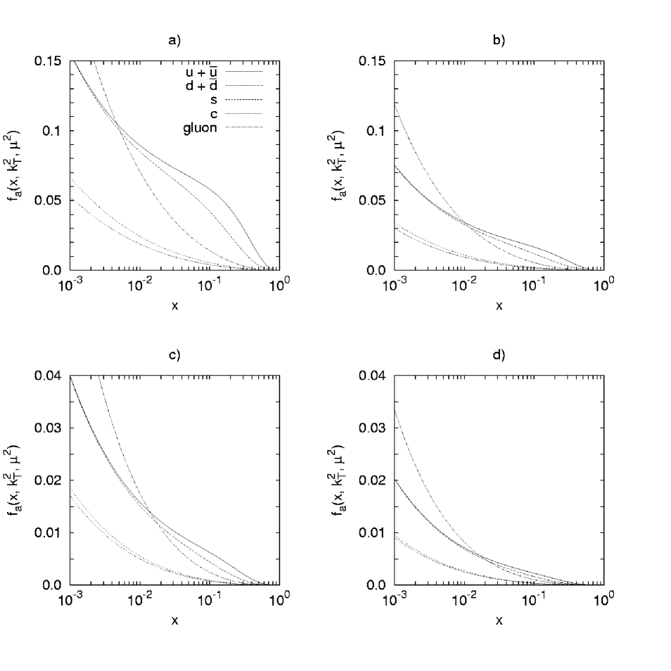
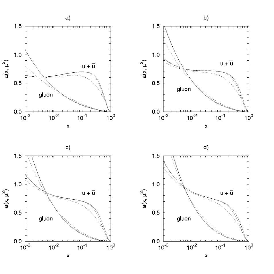
In Figure 1 we show unintegrated parton densities $f_{a}(x,{\mathbf{k}}_{T}^{2},\mu^{2})$ in a proton at scale $\mu^{2}=100\,{\rm GeV}^{2}$ as a function of $x$ for different values of ${\mathbf{k}}_{T}^{2}$, namely ${\mathbf{k}}_{T}^{2}=2\,{\rm GeV}^{2}$ (a), ${\mathbf{k}}_{T}^{2}=5\,{\rm GeV}^{2}$ (b), ${\mathbf{k}}_{T}^{2}=10\,{\rm GeV}^{2}$ (c) and ${\mathbf{k}}_{T}^{2}=20\,{\rm GeV}^{2}$ (d). The solid, dashed, short dashed, dotted and dash-dotted lines correspond to the unintegrated $u+\bar{u}$, $d+\bar{d}$, $s$, $c$ and gluon (divided by factor $10$) distributions, respectively. We have used here the standard GRV (LO) parametrizations [27] of the collinear quark and gluon densities $a(x,\mu^{2})$. In order to be sure that normalization condition (5) is correctly satisfied we have performed the numerical integration of the parton densities $f_{a}(x,{\mathbf{k}}_{T}^{2},\mu^{2})$ over transverse momenta ${\mathbf{k}}_{T}^{2}$. So, in Figure 2 we show our result for effective $u+\bar{u}$ quark and gluon (also divided by factor 10) distributions for different scales $\mu^{2}=2\,{\rm GeV}^{2}$ (a), $\mu^{2}=5\,{\rm GeV}^{2}$ (b), $\mu^{2}=10\,{\rm GeV}^{2}$ (c), $\mu^{2}=20\,{\rm GeV}^{2}$ (d). The solid lines correspond to the effective densities obtained from the unintegrated ones using relation (5). The dashed lines correspond to the collinear GRV (LO) parton distributions. One can see that normalization condition (5) is exactly satisfied practically for all $x$ and $\mu^{2}$ values. There are only rather small (less then few percent) violations of (5) in the case of the $u+\bar{u}$ quark distributions at large $x>0.2$. We have checked numerically that the expression (5) is true also for other parton densities in a proton and in a photon.

For comparison we plot in Figure 2 (as dash-dotted lines) the corresponding LO parton distributions obtained by the CTEQ collaboration [28] (CTEQ5L set). It is clear that there are some differences in both normalization and shape between GRV and CTEQ parametrizations. In general, the CTEQ curves lie below the GRV ones by about $10$%. This difference tends to be small when scale $\mu^{2}$ is large. However, the CTEQ collaboration does not provide a set of the parton distributions in a photon, which are necessary for calculation of the resolved contributions. Therefore everywhere in our numerical analysis we will use only the GRV parametrizations.

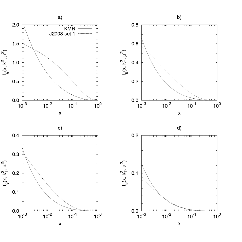
It is interesting to compare the KMR-constructed unintegrated parton densities with the distributions obtained in other approaches. Recently the full CCFM equation in a proton and in a photon was solved numerically using a Monte Carlo method, and new fits of the unintegrated gluon distributions (J2003 set 1 — 3) have been presented [29]. The input parameters were fitted to describe the proton structure function $F_{2}(x,Q^{2})$. These unintegrated gluon densities were used also in description of the forward jet production at HERA, charm and bottom production at Tevatron [29], and charm and $J/\psi$ production at LEP2 energies [30]. In Figure 3 we plot KMR (as solid lines) and J2003 set 1 (as dashed lines) gluon distributions in a proton at scale $\mu^{2}=100\,{\rm GeV}^{2}$ as a function of $x$ for different values of ${\mathbf{k}}_{T}^{2}$, namely ${\mathbf{k}}_{T}^{2}=2\,{\rm GeV}^{2}$ (a), ${\mathbf{k}}_{T}^{2}=10\,{\rm GeV}^{2}$ (b), ${\mathbf{k}}_{T}^{2}=20\,{\rm GeV}^{2}$ (c) and ${\mathbf{k}}_{T}^{2}=50\,{\rm GeV}^{2}$ (d). One can see that J2003 set 1 gluon density is less steep at small $x$ compared to the KMR one. The KMR gluon lie below J2003 set 1 at small ${\mathbf{k}}_{T}^{2}$ region for $x>3\cdot 10^{-3}$. Typically the difference between solid and dashed lines is about 30% — 40% at $x=0.01$. This fact results to the some underestimation of the calculated cross sections in the KMR approach. This underestimation is about 30% at HERA and 50% at Tevatron. Therefore we can expect a rather large sensitivity of our predictions to the parton evolution scheme.

We would like to point out again that behaviour of different unintegrated parton distributions in a proton in the small ${\mathbf{k}}_{T}^{2}$ region (which essentially drives the total cross sections) is very different, as it is clear shown on Figure 3. However, the CCFM evolution does not include quark-initiated chains and therefore can not be used in our analysis since prompt photon production at HERA strongly depends on the quark distributions (see Section 3). Therefore in our following investigations we will use only the KMR unintegrated parton densities. But one should remember that dependence of our results on the evolution scheme may be rather large, and further theoretical attempts (in order to investigate the unintegrated quark distributions more detail) are necessary to reduce this uncertainty.

3 Calculation details

3.1 The subprocesses under consideration

In $ep$ collisions at HERA prompt photons can be produced by one of three mechanisms: a direct production, a single resolved production and via parton-to-photon fragmentation processes [5]. The direct contribution to the $\gamma p\to\gamma+X$ process is the Deep Inelastic Compton (DIC) scattering on the quark (antiquark)

$$\gamma(k_{1})+q(k_{2})\to\gamma(p_{\gamma})+q(p^{\prime}),$$

where the particles four-momenta are given in parentheses. It gives the ${\cal O}(\alpha^{2}_{em})$ order contribution to the hadronic cross section. Here $\alpha_{em}$ is Sommerfeld’s fine structure constant. The single resolved processes are

$$q(k_{1})+g(k_{2})\to\gamma(p_{\gamma})+q(p^{\prime}),$$

$$g(k_{1})+q(k_{2})\to\gamma(p_{\gamma})+q(p^{\prime}),$$

$$q(k_{1})+q(k_{2})\to\gamma(p_{\gamma})+g(p^{\prime}).$$

Since the parton distributions in a photon $a_{\gamma}(x,\mu^{2})$ have a leading behavior proportional to $\alpha_{em}\ln\mu^{2}/\Lambda_{\rm QCD}^{2}\sim\alpha_{em}/\alpha_{s}$, these subprocesses give also the ${\cal O}(\alpha^{2}_{em})$ contributions and therefore should be taken into account in our analysis.

In addition to the direct and resolved production, photons can be also produced through the fragmentation of a hadronic jet into a single photon carrying a large fraction $z$ of the jet energy [5]. These processes are described in terms of quark-to-photon $D_{q\to\gamma}(z,\mu^{2})$ and gluon-to-photon $D_{g\to\gamma}(z,\mu^{2})$ fragmentation functions [7]. The main feature of the fragmentation contribution in leading order is fact that produced photon balanced by a jet on the opposite side of the event and accompanied by collinear hadrons on the same side of the event.

It is very important that in order to reduce the huge background from the secondary photons produced by the decays of $\pi^{0}$, $\eta$ and $\omega$ mesons the isolation criterion is introduced in the experimental analyses. This criterion is the following. A photon is isolated if the amount of hadronic transverse energy $E_{T}^{\rm had}$, deposited inside a cone with aperture $R$ centered around the photon direction in the pseudo-rapidity and azimuthal angle plane, is smaller than some value $E_{T}^{\rm max}$:

$$E_{T}^{\rm had}\leq E_{T}^{\rm max},\atop\displaystyle(\eta-\eta^{\gamma})^{2}+(\phi-\phi^{\gamma})^{2}\leq R^{2}.$$

The both H1 and ZEUS collaborations take $R=1$, $E_{T}^{\rm max}=\epsilon E_{T}^{\gamma}$ with $\epsilon=0.1$ in the experiment [1–4]. Isolation not only reduces the background but also significantly reduces the fragmentation components. It was shown [7] that after applying the isolation cut (11) the contribution from the fragmentation subprocesses is about 5 — 6% of the total cross section. Since the dependence of our results on the non-collinear parton evolution scheme may be rather large (as it was demonstrated in Section 2), in our further analysis we will neglect the relative small fragmentation contribution and consider only the direct and resolved production (7) — (10). We note that photon produced in these processes is automatically isolated from the quark or gluon jet by requiring a non-zero transverse momentum of a photon or jet in the $\gamma p$ center-of-mass frame.

It was claimed [7, 25] that direct box diagram $\gamma g\to\gamma g$, which is formally of the next-to-next-to-leading order (NNLO), gives approximately 6% contribution to the total NLO cross section. In the present paper we will not take into account this diagram also.

3.2 Cross section for prompt photon production

Let $p_{e}$ and $p_{p}$ be the four-momenta of the initial electron and proton. The direct contribution (7) to the $\gamma p\to\gamma+X$ process in the $k_{T}$-factorization approach can be written as

$$d\sigma^{\rm(dir)}(\gamma p\to\gamma+X)=\sum_{q}\int{dx_{2}\over x_{2}}f_{q}(x_{2},{\mathbf{k}}_{2T}^{2},\mu^{2})d{\mathbf{k}}_{T}^{2}{d\phi_{2}\over 2\pi}d{\hat{\sigma}}(\gamma q\to\gamma q),$$

where ${\hat{\sigma}}(\gamma q\to\gamma q)$ is the hard subprocess cross section via quark or antiquark having fraction $x_{2}$ of a initial proton longitudinal momentum, non-zero transverse momentum ${\mathbf{k}}_{2T}$ (${\mathbf{k}}_{2T}^{2}=-k_{2T}^{2}\neq 0$) and azimuthal angle $\phi_{2}$. The expression (12) can be easily rewritten in the form

$$\sigma^{\rm(dir)}(\gamma p\to\gamma+X)=\sum_{q}\int{E_{T}^{\gamma}\over 8\pi(x_{2}s)^{2}(1-\alpha)}|\bar{\cal M}|^{2}(\gamma q\to\gamma q)\times\atop\displaystyle\times f_{q}(x_{2},{\mathbf{k}}_{2T}^{2},\mu^{2})dy^{\gamma}dE_{T}^{\gamma}d{\mathbf{k}}_{2T}^{2}{d\phi_{2}\over 2\pi}{d\phi^{\gamma}\over 2\pi},$$

where $|\bar{\cal M}|^{2}(\gamma q\to\gamma q)$ is the hard matrix element which depends on the transverse momentum ${\mathbf{k}}_{2T}^{2}$, $s=(k_{1}+p_{p})^{2}$ is the total energy of the subprocess under consideration, $y^{\gamma}$, $E_{T}^{\gamma}$ and $\phi^{\gamma}$ are the rapidity, transverse energy and azimuthal angle of the produced photon in the $\gamma p$ center-of-mass frame, and $\alpha=E_{T}^{\gamma}\exp y^{\gamma}/\sqrt{s}$.

The formula for the resolved contribution to the prompt photon photoproduction in the $k_{T}$-factorization approach can be obtained by the similar way. But one should keep in mind that convolution in (12) should be made also with the unintegrated parton distributions $f_{a}^{\gamma}(x,{\mathbf{k}}_{T}^{2},\mu^{2})$ in a photon, i.e.

$$d\sigma^{\rm(res)}(\gamma p\to\gamma+X)=\sum_{a,b}\int{dx_{1}\over x_{1}}f_{a}^{\gamma}(x_{1},{\mathbf{k}}_{1T}^{2},\mu^{2})d{\mathbf{k}}_{1T}^{2}{d\phi_{1}\over 2\pi}\times\atop\displaystyle\times\int{dx_{2}\over x_{2}}f_{b}(x_{2},{\mathbf{k}}_{2T}^{2},\mu^{2})d{\mathbf{k}}_{2T}^{2}{d\phi_{2}\over 2\pi}d{\hat{\sigma}}(ab\to\gamma c),$$

where $a,b,c=q$ and/or $g$, ${\hat{\sigma}}(ab\to\gamma c)$ is the cross section of the photon production in the corresponding parton-parton interaction (8) — (10). Here parton $a$ has fraction $x_{1}$ of a initial photon longitudinal momentum, non-zero transverse momentum ${\mathbf{k}}_{1T}$ (${\mathbf{k}}_{1T}^{2}=-k_{1T}^{2}\neq 0$) and azimuthal angle $\phi_{1}$. We can easily obtain the final expression from equation (14). It has the form

$$\sigma^{\rm(res)}(\gamma p\to\gamma+X)=\sum_{a,b}\int{E_{T}^{\gamma}\over 8\pi(x_{1}x_{2}s)^{2}}|\bar{\cal M}|^{2}(ab\to\gamma c)\times\atop\displaystyle\times f_{a}^{\gamma}(x_{1},{\mathbf{k}}_{1T}^{2},\mu^{2})f_{b}(x_{2},{\mathbf{k}}_{2T}^{2},\mu^{2})d{\mathbf{k}}_{1T}^{2}d{\mathbf{k}}_{2T}^{2}dE_{T}^{\gamma}dy^{\gamma}dy^{c}{d\phi_{1}\over 2\pi}{d\phi_{2}\over 2\pi}{d\phi^{\gamma}\over 2\pi},$$

where $y^{c}$ is the rapidity of the parton $c$ in the $\gamma p$ center-of-mass frame. It is important that hard matrix elements $|\bar{\cal M}|^{2}(ab\to\gamma c)$ depend on the transverse momenta ${\mathbf{k}}_{1T}^{2}$ and ${\mathbf{k}}_{2T}^{2}$. We would like to note that if we average the expressions (13) and (15) over ${\mathbf{k}}_{1T}$ and ${\mathbf{k}}_{2T}$ and take the limit ${\mathbf{k}}_{1T}^{2}\to 0$ and ${\mathbf{k}}_{2T}^{2}\to 0$, then we obtain well-known expressions for the prompt photon production in leading-order (LO) perturbative QCD.

The experimental data taken by the H1 [4] and ZEUS [3] collaborations refer to the prompt photon production in the $ep$ collisions, where electron is scattered at small angle and the mediating photon is almost real ($Q^{2}\sim 0$). Therefore $\gamma p$ cross sections (13) and (15) needs to be weighted with the photon flux in the electron:

$$d\sigma(ep\to e^{\prime}+\gamma+X)=\int f_{\gamma/e}(y)d\sigma(\gamma p\to\gamma+X)dy,$$

where $y$ is a fraction of the initial electron energy taken by the photon in the laboratory frame, and we use the Weizacker-Williams approximation for the bremsstrahlung photon distribution from an electron:

$$f_{\gamma/e}(y)={\alpha_{em}\over 2\pi}\left({1+(1-y)^{2}\over y}\ln{Q^{2}_{\rm max}\over Q^{2}_{\rm min}}+2m_{e}^{2}y\left({1\over Q^{2}_{\rm max}}-{1\over Q^{2}_{\rm min}}\right)\right).$$

Here $m_{e}$ is the electron mass, $Q^{2}_{\rm min}=m_{e}^{2}y^{2}/(1-y)^{2}$ and $Q^{2}_{\rm max}=1\,{\rm GeV}^{2}$, which is a typical value for the recent photoproduction measurements at the HERA collider.

The multidimensional integration in (13), (15) and (16) has been performed by means of the Monte Carlo technique, using the routine VEGAS [31]. The full C$++$ code is available from the authors on request. For reader’s convenience, we collect the analytic expressions for the off-shell matrix elements which correspond to all partonic subprocesses under consideration (7) — (10) in the Appendix. These formulas may be useful for the subsequent applications.

4 Numerical results

We now are in a position to present our numerical results. First we describe our theoretical input and the kinematical conditions. After we fixed the unintegrated parton distributions in a proton $f_{a}(x,{\mathbf{k}}_{T}^{2},\mu^{2})$ and in a photon $f_{a}^{\gamma}(x,{\mathbf{k}}_{T}^{2},\mu^{2})$, the cross sections (13) and (15) depend on the energy scale $\mu$. As it often done [7, 25] for prompt photon production, we choose the renormalization and factorization scales to be $\mu=\xi E_{T}^{\gamma}$. In order to estimate the theoretical uncertainties of our calculations we will vary the scale parameter $\xi$ between 1/2 and 2 about the default value $\xi=1$. Also we use LO formula for the strong coupling constant $\alpha_{s}(\mu^{2})$ with $n_{f}=3$ active (massless) quark flavours and $\Lambda_{\rm QCD}=232$ MeV, such that $\alpha_{s}(M_{Z}^{2})=0.1169$. In our analysis we will not neglect the charm quark mass and set it to be $m_{c}=1.4$ GeV.

4.1 Inclusive prompt photon production

Experimental data for the inclusive prompt photon production $ep\to e^{\prime}+\gamma+X$ comes from both ZEUS and H1 collaborations. Two differential cross section are determined: first as a function of the transverse energy $E_{T}^{\gamma}$, and second as a function of pseudo-rapidity $\eta^{\gamma}$. The ZEUS data [3] refer to the kinematic region defined by $5<E_{T}^{\gamma}<10$ GeV and $-0.7<\eta^{\gamma}<0.9$ with electron energy $E_{e}=27.5$ GeV and proton energy $E_{p}=820$ GeV. The fraction $y$ of the electron energy trasferred to the photon is restricted to the range $0.2<y<0.9$. Additionally the available ZEUS data for the prompt photon pseudo-rapidity distributions have been given also for three subdivisons of the $y$ range, namely $0.2<y<0.32$ ($134<W<170$ GeV), $0.32<y<0.5$ ($170<W<212$ GeV) and $0.5<y<0.9$ ($212<W<285$ GeV). The more recent H1 data [4] refer to the kinematic region defined by $5<E_{T}^{\gamma}<10$ GeV, $-1<\eta^{\gamma}<0.9$ and $0.2<y<0.7$ with electron energy $E_{e}=27.6$ GeV and proton energy $E_{p}=920$ GeV.

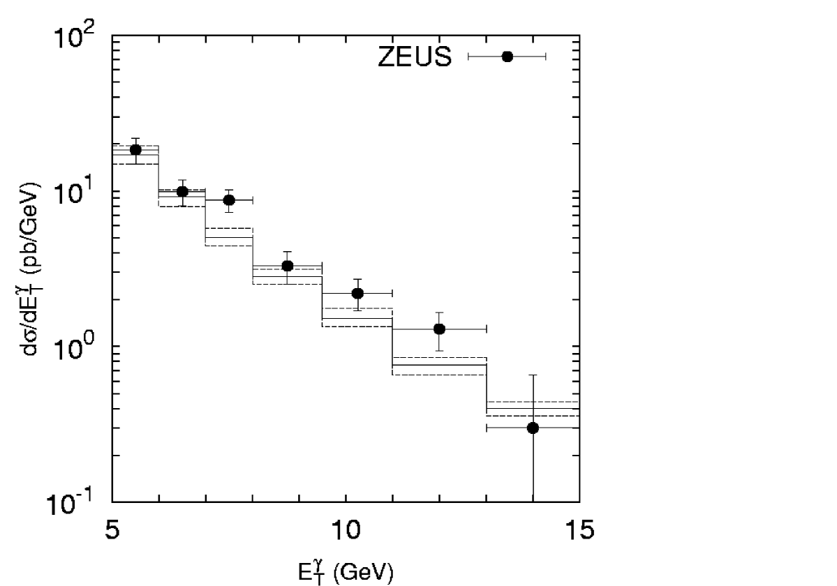
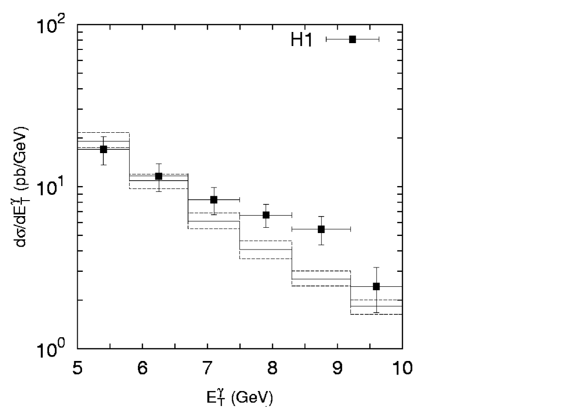
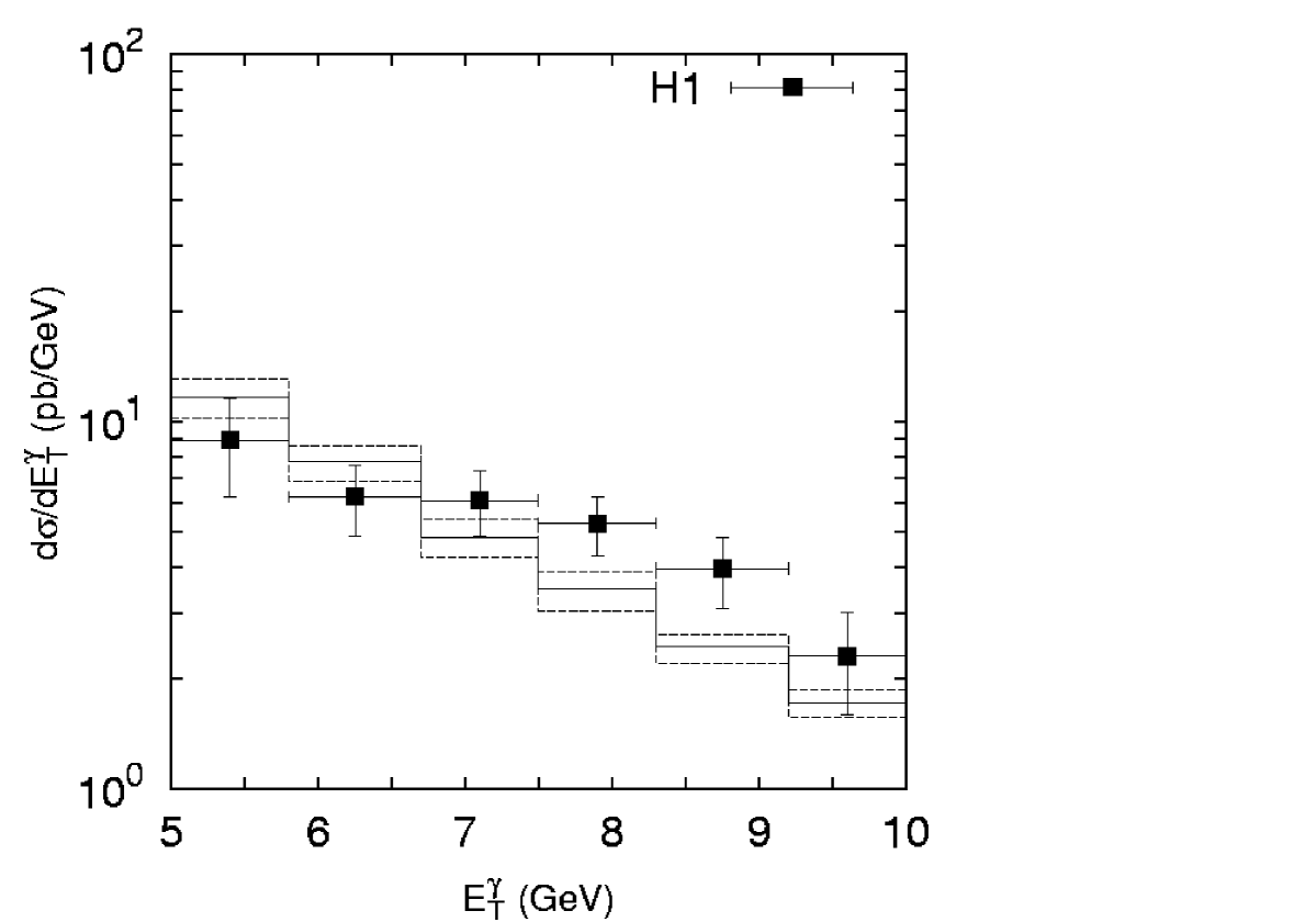
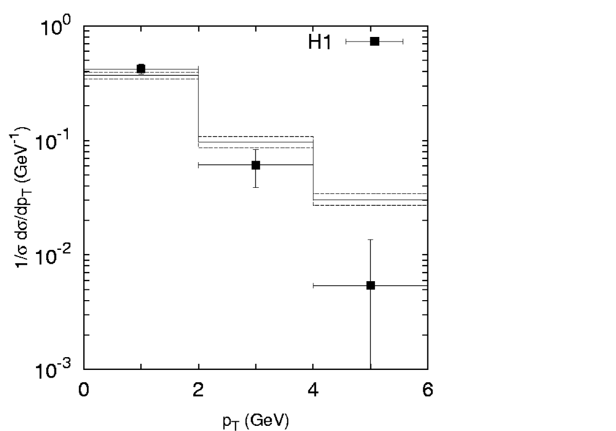
The transverse energy distributions of the inclusive prompt photon for different kinematical region are shown in Figures 4 and 5 in comparison to the HERA data. Instead of presenting our theoretical predictions as continuous lines, we adopt the binning pattern encoded in the experimental data. The solid histograms obtained by fixing both the factorization and normalization scales at the default value $\mu=E_{T}^{\gamma}$, whereas upper and lower dashed histograms correspond to the $\mu=E_{T}^{\gamma}/2$ and $\mu=2E_{T}^{\gamma}$ scales, respectively. One can see that predicted cross sections agree well with the experimental data except the moderate $E_{T}^{\gamma}$ region. We would like to note that overall agreement with data can be improved when unintegrated quark and gluon distributions in a proton and in a photon will be studied more detail. It is because the KMR approach tends to underestimate the calculated cross sections, as it was discussed in Section 2. The collinear NLO QCD calculations [7, 25] give the similar description of the transverse energy distributions measured by the ZEUS collaboration. At the same time, according to the analysis which was done by the H1 collaboration [4], in order to obtain a realistic comparison of their data and theory the corrections for hadronisation and multiple interactions should be taken into account in the predictions. The correction factors are typically 0.7 — 0.9 depending on a bin. The NLO calculations [7, 25] are approximately 30% — 40% below the H1 data if the corrections for hadronisation and multiple interactions are applied. We would like to note that these corrections are not accounted for in our analysis. The effect of scale variations in transverse energy distributions is rather large: the relative difference between results for $\mu=E_{T}^{\gamma}$ and results for $\mu=E_{T}^{\gamma}/2$ or $\mu=2E_{T}^{\gamma}$ is about 15%.

The pseudo-rapidity distributions of the inclusive prompt photon production compared with the HERA data in different kinematical region are shown in Figures 6 and 7. All histograms here are the same as in Figure 4. One can see that measured distributions are reasonably well described in the pseudo-rapidity region $-0.4\leq\eta^{\gamma}\leq 0.9$ only. For $-1\leq\eta^{\gamma}\leq-0.4$ our predictions lie mostly below the experimental points. The discrepancy between data and theory at negative $\eta^{\gamma}$ is found to be relative strong at low values of the initial photon fractional momentum $y$. So, in Figures 8, 9 and 10 we show the inclusive cross sections $d\sigma/d\eta^{\gamma}$ evaluated for the three $y$ ranges $0.2<y<0.32$ ($134<W<170$ GeV), $0.32<y<0.5$ ($170<W<212$ GeV) and $0.5<y<0.9$ ($212<W<285$ GeV), respectively. All histograms here are the same as in Figure 4. In the lowest $y$ range, both our predictions and experimental data show a peaking at negative $\eta^{\gamma}$, but it is stronger in the data. In the high $y$ region, $0.5<y<0.9$, a good agreement is obtained. This fact allows to establish that the above discussed discrepancy between the data and theory at $-1\leq\eta^{\gamma}\leq-0.4$ is coming from the low ($0.2<y<0.32$) and medium ($0.32<y<0.5$) $y$ region. The scale variation changes the estimated cross sections by about 15%. The collinear NLO QCD calculations [7, 25] give the similar description of the pseudo-rapidity distributions measured by the ZEUS collaboration. At the same time, after corrections for hadronisation and multiple interactions (not accounted for in our analysis) the NLO predictions are 30% — 40% below the H1 data.

As it was already mentioned above, the dependence of the our results on a renormalization/factorization scale $\mu$ is rather large, about 10% — 15% in the wide kinematic range. There are also additional uncertainties come from the unintegrated parton densities, as it was discussed in Section 2. The theoretical uncertainties of the collinear NLO QCD calculations are about 3% [7, 25]. This fact indicates that contribution from NNLO and high order terms is not significant. At the same time the strong scale dependence of our results demonstrates the necessarity of reducing of uncertainties in the non-collinear parton evolution.

The individual contributions from the direct and resolved production mechanisms to the total cross section in the $k_{T}$-factorization approach is about 47% and 53%, respectively. In the resolved conribution, the channels (8), (9) and (10) account for 80%, 14% and 6%. Additionally, using the Duke-Owens (DO) [32] parton-to-photon fragmentation functions, we perform the estimation of the fragmentation component (not shown in Figures). We find that after applying isolation cut it give only a very small (about few percent) contribution.

4.2 Prompt photon production in association with jet

Now we demonstrate how $k_{T}$-factorization approach can be used to calculate the semi-inclusive prompt photon production rates. The produced photon is accompanied by a number of partons radiated in the course of the parton evolution. As it has been noted in Ref. [33], on the average the parton transverse momentum decreases from the hard interaction block towards the proton. As an approximation, we assume that the parton $k^{\prime}$ emitted in the last evolution step compensates the whole transverse momentum of the parton participating in the hard subprocess, i.e. ${\mathbf{k}^{\prime}}_{T}\simeq-{\mathbf{k}}_{T}$. All the other emitted partons are collected together in the proton remnant, which is assumed to carry only a negligible transverse momentum compared to ${\mathbf{k}^{\prime}}_{T}$. This parton gives rise to a final hadron jet with $E_{T}^{\rm jet}=|{\mathbf{k}^{\prime}}_{T}|$ in addition to the jet produced in the hard subprocess. From these hadron jets we choose the one carrying the largest transverse energy, and then compute prompt photon with an associated jet cross sections.

Experimental data for such processes were obtained [4] very recently by the H1 collaboration. The cross sections measured differentially as a function of $E_{T}^{\gamma}$, $E_{T}^{\rm jet}$, and the pseudo-rapidities $\eta^{\gamma}$ and $\eta^{\rm jet}$ in the kinematic region defined by $5<E_{T}^{\gamma}<10$ GeV, $E_{T}^{\rm jet}>4.5$ GeV, $-1<\eta^{\gamma}<0.9$, $-1<\eta^{\rm jet}<2.3$ and $0.2<y<0.7$ with electron energy $E_{e}=27.6$ GeV and proton energy $E_{p}=920$ GeV. There are no ZEUS data for the prompt photon plus jet production, although some data for distribution of events, not corrected for the detector effects, were presented [2].

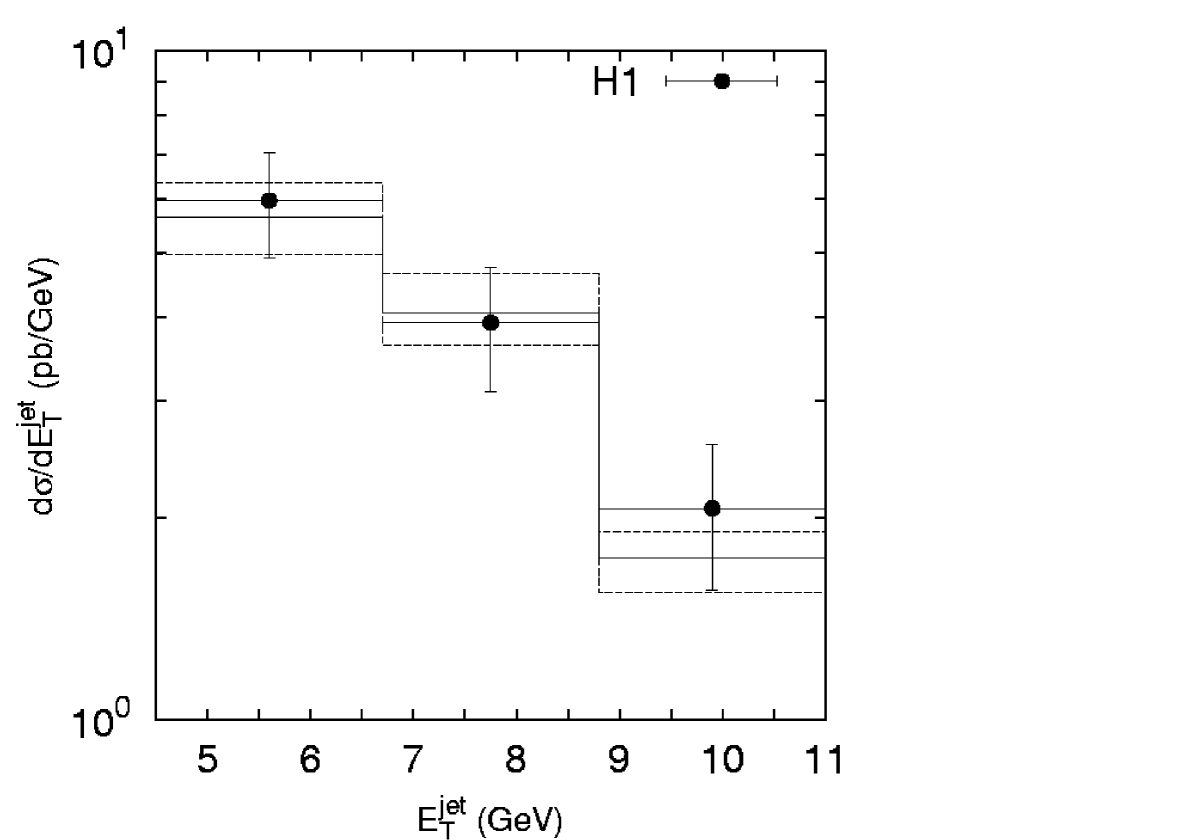
The transverse energy $E_{T}^{\gamma}$ and pseudo-rapidity $\eta^{\gamma}$ distributions of the prompt photon plus jet production are shown in Figures 11 and 12 in comparison with H1 data. All histograms here are the same as in Figure 4. In contrast to the inclusive case, one can see that our predictions are consistent with the data in most bins, although some discrepancies are present. The scale variation as it was described above changes the estimated cross sections by about 10%. The results of the collinear NLO calculations [7, 25] which include corrections for hadronisation and multiple interactions give the similar results and consistent with data also.

In Figures 13 and 14 we show our predictions for the transverse energy $E_{T}^{\rm jet}$ and pseudo-rapidity $\eta^{\rm jet}$ distributions in comparison with H1 data. All histograms here are the same as in Figure 4. A rather good agreement between our results and data is obtained again. It is interesting to note that shape of the predicted pseudo-rapidity $\eta^{\rm jet}$ distribution coincide with the one obtained in the collinear NLO calculations [7, 25]. At the same time the shape of this distribution is not reproduced by the leading-order QCD calculations [4]. This fact can demonstrate again that the main part of the collinear high-order corrections is already included at LO level in $k_{T}$-factorization formalism. The scale dependence of our predictions is about 10%.

The most important variables for testing the structure of colliding proton and photon are the longitudinal fractional momenta of partons in these particles. In order to reconstruct the momentum fractions of the initial partons from measured quantities the observables $x_{\gamma}$ and $x_{p}$ are introduced [4]:

$$x_{\gamma}={E_{T}^{\gamma}(e^{-\eta^{\gamma}}+e^{-\eta^{\rm jet}})\over 2yE_{e}},\quad\displaystyle x_{p}={E_{T}^{\gamma}(e^{\eta^{\gamma}}+e^{\eta^{\rm jet}})\over 2E_{p}}.$$

These observables make explicit use only of the photon energy, which is better measured than the jet energy. The $x_{\gamma}$ distribution is particularly sensitive to the photon structure function. At large $x_{\gamma}$ region ($x_{\gamma}>0.85$) the cross section is dominated by the contribution of processes with direct initial photons, whereas at $x_{\gamma}<0.85$ the resolved photon contributions dominate [4].

So, in Figures 15 and 16 the $x_{\gamma}$ and $x_{p}$ distributions are shown in comparison with H1 data. One can see that our predictions reasonable agree with experimental data. The NLO calculations [7, 25] without corrections for hadronisation and multiple interactions give the similar results. However, NLO calculations tend to underestimate the H1 data if these corrections are taken into account. The hadronic and multiple interaction corrections improve the description of the data at $x_{\gamma}<0.6$ only [4].

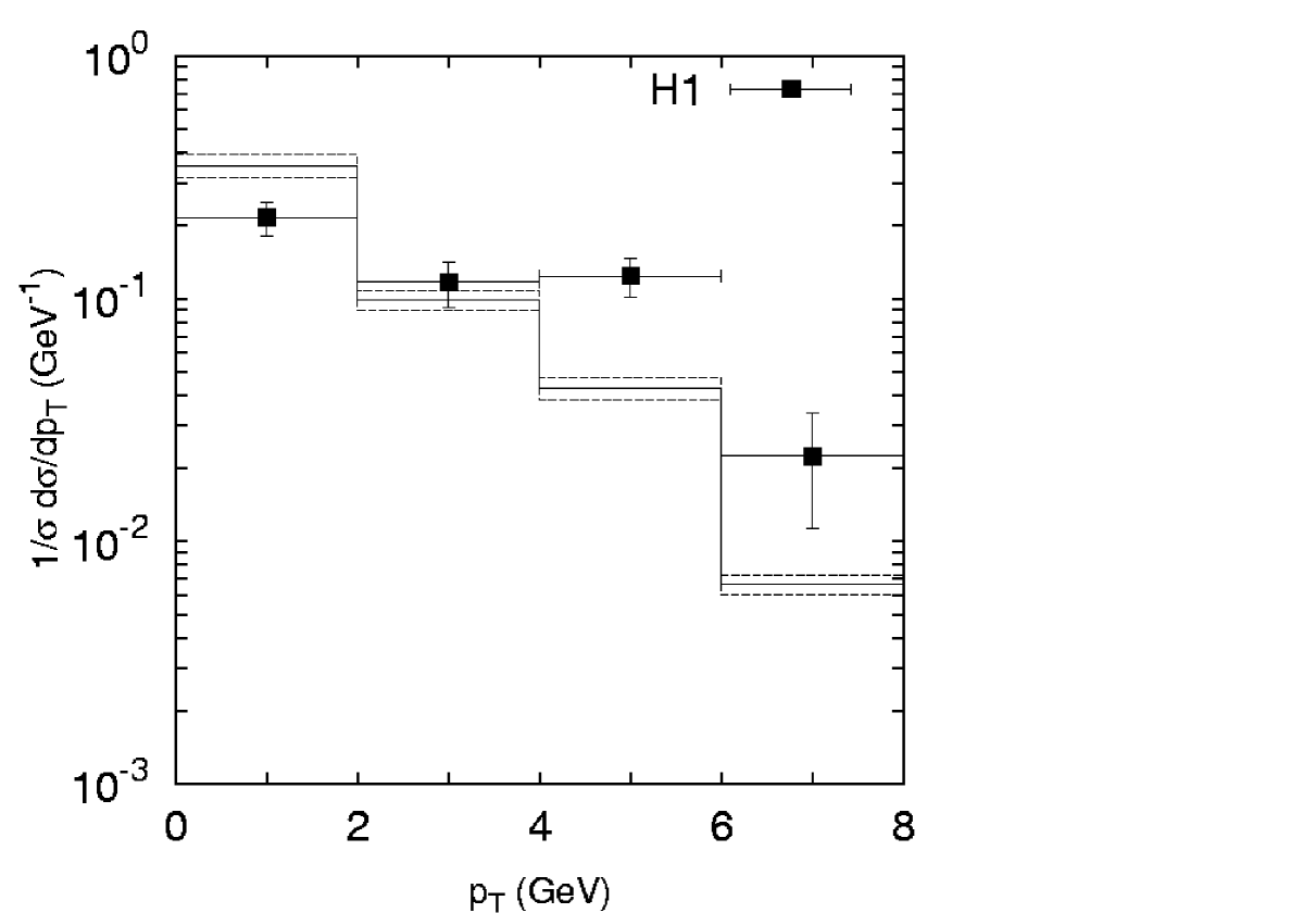
Further understanding of the process dynamics and in particular of the high-order correction effects may be obtained from the transverse correlation between the produced prompt photon and the jet. The H1 collaboration has measured the distribution on the component of the prompt photon’s momentum perpendicular to the jet direction in the transverse plane, i.e.

$$p_{T}=|{\mathbf{p}}_{T}^{\gamma}\times{\mathbf{p}}_{T}^{\rm jet}|/|{\mathbf{p}}_{T}^{\rm jet}|=E_{T}^{\gamma}\sin\Delta\phi,$$

where $\Delta\phi$ is the difference in azimuth between the photon and the jet. In the collinear leading order approximation, the distribution over $p_{T}$ must be simply a delta function $\delta(p_{T})$, since the produced photon and the jet are back-to-back in the transverse plane. Taking into account the non-vanishing initial parton transverse momenta ${\mathbf{k}}_{1T}$ and ${\mathbf{k}}_{2T}$ leads to the violation of this back-to-back kinematics in the $k_{T}$-factorization approach.

The normalised $p_{T}$ distributions are shown in Figures 17 and 18 separately for the regions $x_{\gamma}<0.85$ and $x_{\gamma}>0.85$, where direct and resolved photon induced processes dominate, respectively. All histograms here are the same as in Figure 4. Our predictions are consistent with the H1 data for all $x_{\gamma}$ values except large $p_{T}$ region. So, at $p_{T}>5$ GeV the results of our calculations lie slightly below the data at $x_{\gamma}<0.85$ and above the data at $x_{\gamma}>0.85$. At the same time the NLO QCD prediction [7] gives a better description of the $p_{T}$ distributions at $x_{\gamma}<0.85$ than another one [25]. It is because in this region the cross section is dominated by ${\cal O}(\alpha_{s})$ corrections to the processes with resolved photons, which are not included in the NLO calculations [25]. In general, we can conclude that our results lie between the predictions [7] and the predictions [25] in the whole $x_{\gamma}$ range. This fact indicates again that the main part of the high-order collinear corrections is effectively included in our calculations.

Finally, we would like to note that there are, of course, still rather large theoretical uncertainties in our results connected with unintegrated parton distributions, and it is necessary to work hard until these uncertainties will be reduced. However, it was shown [24] that the properties of different unintegrated parton distributions clear manifest themselves in the azimuthal correlation between transverse momenta of the final state particles. Therefore we can expect that further theoretical and experimental studying of these correlations will give important information about non-collinear parton evolution dynamics in a proton and in a photon.

5 Conclusions

We have investigated the prompt photon photoproduction at the HERA collider in the $k_{T}$-factorization approach. In order to obtain the unintegrated quark and gluon distributions in a proton and in a photon we used the Kimber-Martin-Ryskin prescription. We have investigated both inclusive and associated with jet prompt photon production rates. Such calculations in the $k_{T}$-factorization approach were performed for the first time.

We took into account both the direct and resolved contributions and investigated the sensitivity of the our results to renormalization and factorization scales. There are, of course, also theoretical uncertainties due to non-collinear evolution scheme. However, much more work needs to be done before these uncertainties will be reduced.

We have found that our predictions for the inclusive prompt photon production are in reasonable agreement with the H1 and ZEUS data except rear (electron direction) pseudo-rapidity region. In contrast, our results for prompt photon associated with jet are consistent with data in the whole kinematical range. However, the scale dependence of our results is rather large compared to the collinear NLO QCD calculations. At the same time we demonstrate that main part of the standard high-order corrections is already included in the $k_{T}$-factorization formalism at LO level.

Note that in our analysis we neglect the contribution from the fragmentation processes and from the direct box diagram ($\gamma g\to\gamma g$). Since the relative large box contribution (about 6% of the total NLO cross section) is mainly due to large gluonic content of the proton at small $x$, studying of this subprocess should be also very interesting in the $k_{T}$-factorization approach. We plan to investigate it in detail in the forthcoming publications.

6 Acknowledgements

The authors are very grateful also to S.P. Baranov for encouraging interest and helpful discussions. This research was supported in part by the FASI of Russian Federation.

7 Appendix

Here we present the compact analytic expressions for the hard matrix elements which appear in (13) and (15). In the following, $\hat{s}$, $\hat{t}$ and $\hat{u}$ are usual Mandelstam variables for corresponding $2\to 2$ subprocesses and $e_{q}$ is the fractional electric charge of quark $q$.

We start from the direct subprocess (7). The corresponding squared matrix element summed over final polarization states and averaged over initial ones read

$$|\bar{\cal M}|^{2}(\gamma q\to\gamma q)={\displaystyle 2(4\pi)^{2}\alpha_{em}^{2}e_{q}^{4}\over\displaystyle(\hat{s}-m^{2})^{2}(\hat{u}-m^{2})^{2}}F_{\gamma q}({\mathbf{k}}_{2T}^{2}),$$

where $m$ is the quark mass, and

$$F_{\gamma q}({\mathbf{k}}_{T}^{2})=6m^{8}-(3\hat{s}^{2}+14\hat{s}\hat{u}+3\hat{u}^{2})m^{4}+(\hat{s}^{3}+7\hat{s}^{2}\hat{u}+\atop 7\hat{u}^{2}\hat{s}+\hat{u}^{3})m^{2}-(\hat{s}^{2}+\hat{u}^{2})\hat{s}\hat{u}.$$

It is important to note that when we calculate the Dirac’s traces we set the incoming quark four-momentum to be equal $k_{2}=x_{2}p_{p}$. Therefore these formulas formally are the same as in the usual leading-order collinear approach and there is no obvious dependence on the parton transverse momentum ${\mathbf{k}}_{2T}$. However, this dependence is present because we have used true off-shell kinematics in order to estimate the cross section (13). It is in the clear contrast with the collinear calculations.

The squared matrix elements of the resolved photon contributions (8) — (10) summed over final polarization states and averaged over initial ones read

$$|\bar{\cal M}|^{2}(qg\to\gamma q)={\displaystyle(4\pi)^{2}\alpha_{em}\alpha_{s}e_{q}^{2}\over\displaystyle 3(\hat{t}-m^{2})^{2}(\hat{s}-m^{2})^{2}}F_{qg}({\mathbf{k}}_{1T}^{2},{\mathbf{k}}_{2T}^{2}),$$

$$|\bar{\cal M}|^{2}(gq\to\gamma q)={\displaystyle(4\pi)^{2}\alpha_{em}\alpha_{s}e_{q}^{2}\over\displaystyle 3(\hat{s}-m^{2})^{2}(\hat{u}-m^{2})^{2}}F_{gq}({\mathbf{k}}_{1T}^{2},{\mathbf{k}}_{2T}^{2}),$$

$$|\bar{\cal M}|^{2}(qq\to\gamma g)=-{\displaystyle 8(4\pi)^{2}\alpha_{em}\alpha_{s}e_{q}^{2}\over\displaystyle 9(\hat{t}-m^{2})^{2}(\hat{u}-m^{2})^{2}}F_{qq}({\mathbf{k}}_{1T}^{2},{\mathbf{k}}_{2T}^{2}),$$

where functions $F_{qg}({\mathbf{k}}_{1T}^{2},{\mathbf{k}}_{2T}^{2})$, $F_{gq}({\mathbf{k}}_{1T}^{2},{\mathbf{k}}_{2T}^{2})$ and $F_{qq}({\mathbf{k}}_{1T}^{2},{\mathbf{k}}_{2T}^{2})$ are given by

$$F_{qg}({\mathbf{k}}_{1T}^{2},{\mathbf{k}}_{2T}^{2})=6m^{8}-(2{\mathbf{k}}_{2T}^{4}+2(\hat{s}+\hat{t}){\mathbf{k}}_{2T}^{2}+3\hat{s}^{2}+3\hat{t}^{2}+14\hat{s}\hat{t})m^{4}+$$

$$(2(\hat{s}+\hat{t}){\mathbf{k}}_{2T}^{4}+8\hat{s}\hat{t}{\mathbf{k}}_{2T}^{2}+\hat{s}^{3}+\hat{t}^{3}+7\hat{s}\hat{t}^{2}+7\hat{s}^{2}\hat{t})m^{2}-$$

$$\hat{s}\hat{t}(2{\mathbf{k}}_{2T}^{4}+2(\hat{s}+\hat{t}){\mathbf{k}}_{2T}^{2}+\hat{s}^{2}+\hat{t}^{2}),$$

$$F_{gq}({\mathbf{k}}_{1T}^{2},{\mathbf{k}}_{2T}^{2})=6m^{8}-(2{\mathbf{k}}_{1T}^{4}+2(\hat{s}+\hat{u}){\mathbf{k}}_{1T}^{2}+3\hat{s}^{2}+3\hat{u}^{2}+14\hat{s}\hat{u})m^{4}+$$

$$(2(\hat{s}+\hat{u}){\mathbf{k}}_{1T}^{4}+8\hat{s}\hat{u}{\mathbf{k}}_{1T}^{2}+\hat{s}^{3}+\hat{u}^{3}+7\hat{s}\hat{u}^{2}+7\hat{s}^{2}\hat{u})m^{2}-$$

$$\hat{s}\hat{u}(2{\mathbf{k}}_{1T}^{4}+2(\hat{s}+\hat{u}){\mathbf{k}}_{1T}^{2}+\hat{s}^{2}+\hat{u}^{2}),$$

$$F_{qq}({\mathbf{k}}_{1T}^{2},{\mathbf{k}}_{2T}^{2})=6m^{8}-(3\hat{t}^{2}+3\hat{u}^{2}+14\hat{t}\hat{u})m^{4}+(\hat{t}^{3}+\hat{u}^{3}+\atop 7\hat{t}\hat{u}^{2}+7\hat{t}^{2}\hat{u})m^{2}-\hat{t}\hat{u}(\hat{t}^{2}+\hat{u}^{2}).$$

Since we take into account the ${\mathbf{k}}_{T}$ depencence of the incoming virtual gluon polarization tensor, the functions $F_{qg}({\mathbf{k}}_{1T}^{2},{\mathbf{k}}_{2T}^{2})$ and $F_{gq}({\mathbf{k}}_{1T}^{2},{\mathbf{k}}_{2T}^{2})$ also depend obviously on the gluon transverse momentum. It is clear that if we take the limit ${\mathbf{k}}_{1T}^{2}\to 0$, ${\mathbf{k}}_{2T}^{2}\to 0$ in (A.1) — (A.8) we easily obtain the corresponding collinear formulas.

Finally, we would like to point out again that in numerical computations we use precise off-shell kinematics and therefore all expressions (A.1) — (A.8) depends on the parton transverse momentum. In particular, the incident parton momentum fractions $x_{1}$ and $x_{2}$ in (13) and (15) have some ${\mathbf{k}}_{T}$ dependence. In the limit ${\mathbf{k}}_{1T}\to 0$, ${\mathbf{k}}_{2T}\to 0$ we reproduce standard leading-order QCD collinear results.

Figure 1: The unintegrated parton distributions $f_{a}(x,{\mathbf{k}}_{T}^{2},\mu^{2})$ at scale $\mu^{2}=100\,{\rm GeV}^{2}$ as a function of $x$ for different values of ${\mathbf{k}}_{T}^{2}$, namely ${\mathbf{k}}_{T}^{2}=2\,{\rm GeV}^{2}$ (a), ${\mathbf{k}}_{T}^{2}=5\,{\rm GeV}^{2}$ (b), ${\mathbf{k}}_{T}^{2}=10\,{\rm GeV}^{2}$ (c) and ${\mathbf{k}}_{T}^{2}=20\,{\rm GeV}^{2}$ (d). The solid, dashed, short dashed, dotted and dash-dotted lines correspond to the unintegrated $u+\bar{u}$, $d+\bar{d}$, $s$, $c$ and gluon (divided by factor $10$) distributions, respectively.

Figure 2: The effective parton distributions $a(x,\mu^{2})$ as a function of $x$ for different values of $\mu^{2}$, namely $\mu^{2}=2\,{\rm GeV}^{2}$ (a), $\mu^{2}=5\,{\rm GeV}^{2}$ (b), $\mu^{2}=10\,{\rm GeV}^{2}$ (c) and $\mu^{2}=20\,{\rm GeV}^{2}$ (d). The solid lines correspond to the parton densities taken from the unintegrated ones using relation (5). The dashed and dash-dotted lines correspond to the conventional GRV (LO) and CTEQ5L parton distributions, respectively. Everywhere the gluon distributions are divided by factor $10$.

Figure 3: The unitegrated gluon distributions $f_{g}(x,{\mathbf{k}}_{T}^{2},\mu^{2})$ at scale $\mu^{2}=100\,{\rm GeV}^{2}$ as a function of $x$ for different values of ${\mathbf{k}}_{T}^{2}$, namely ${\mathbf{k}}_{T}^{2}=2\,{\rm GeV}^{2}$ (a), ${\mathbf{k}}_{T}^{2}=10\,{\rm GeV}^{2}$ (b), ${\mathbf{k}}_{T}^{2}=20\,{\rm GeV}^{2}$ (c) and ${\mathbf{k}}_{T}^{2}=50\,{\rm GeV}^{2}$ (d). The solid lines and dashed lines correspond to the KMR and J2003 set 1 gluon densities, respectively.

Figure 4: The differential cross section $d\sigma/dE_{T}^{\gamma}$ for the inclusive prompt photon production calculated at $-0.7<\eta^{\gamma}<0.9$ and $0.2<y<0.9$. The solid histogram corresponds to the default scale $\mu=E_{T}^{\gamma}$, whereas upper and lower dashed histograms correspond to the $\mu=E_{T}^{\gamma}/2$ and $\mu=2E_{T}^{\gamma}$ scales, respectively. The experimental data are from ZEUS [3].

Figure 5: The differential cross section $d\sigma/dE_{T}^{\gamma}$ for the inclusive prompt photon production calculated at $-1<\eta^{\gamma}<0.9$ and $0.2<y<0.7$. All histograms are the same as in Figure 4. The experimental data are from H1 [4].

Figure 6: The differential cross section $d\sigma/d\eta^{\gamma}$ for the inclusive prompt photon production calculated at $5<E_{T}^{\gamma}<10$ GeV and $0.2<y<0.9$ ($134<W<285$ GeV). All histograms are the same as in Figure 4. The experimental data are from ZEUS [3].

Figure 7: The differential cross section $d\sigma/d\eta^{\gamma}$ for the inclusive prompt photon production calculated at $5<E_{T}^{\gamma}<10$ GeV and $0.2<y<0.7$. All histograms are the same as in Figure 4. The experimental data are from H1 [4].

Figure 8: The differential cross section $d\sigma/d\eta^{\gamma}$ for the inclusive prompt photon production calculated at $5<E_{T}^{\gamma}<10$ GeV and $0.2<y<0.32$ ($134<W<170$ GeV). All histograms are the same as in Figure 4. The experimental data are from ZEUS [3].

Figure 9: The differential cross section $d\sigma/d\eta^{\gamma}$ for the inclusive prompt photon production calculated at $5<E_{T}^{\gamma}<10$ GeV and $0.32<y<0.5$ ($170<W<212$ GeV). All histograms are the same as in Figure 4. The experimental data are from ZEUS [3].

Figure 10: The differential cross section $d\sigma/d\eta^{\gamma}$ for the inclusive prompt photon production calculated at $5<E_{T}^{\gamma}<10$ GeV and $0.5<y<0.9$ ($212<W<285$ GeV). All histograms are the same as in Figure 4. The experimental data are from ZEUS [3].

Figure 11: The differential cross section $d\sigma/dE_{T}^{\gamma}$ for the prompt photon + jet production calculated at $-1<\eta^{\gamma}<0.9$ and $0.2<y<0.7$ with an additional jet requirement $-1<\eta^{\rm jet}<2.3$ and $E_{T}^{\rm jet}>4.5$ GeV. All histograms are the same as in Figure 4. The experimental data are from H1 [4].

Figure 12: The differential cross section $d\sigma/d\eta^{\gamma}$ for the prompt photon + jet production calculated at $5<E_{T}^{\gamma}<10$ GeV and $0.2<y<0.7$ with an additional jet requirement $-1<\eta^{\rm jet}<2.3$ and $E_{T}^{\rm jet}>4.5$ GeV. All histograms are the same as in Figure 4. The experimental data are from H1 [4].

Figure 13: The differential cross section $d\sigma/dE_{T}^{\rm jet}$ for the prompt photon + jet production calculated at $5<E_{T}^{\gamma}<10$ GeV and $0.2<y<0.7$ with an additional jet requirement $-1<\eta^{\rm jet}<2.3$ and $E_{T}^{\rm jet}>4.5$ GeV. All histograms are the same as in Figure 4. The experimental data are from H1 [4].

Figure 14: The differential cross section $d\sigma/d\eta^{\rm jet}$ for the prompt photon + jet production calculated at $5<E_{T}^{\gamma}<10$ GeV and $0.2<y<0.7$ with an additional jet requirement $-1<\eta^{\rm jet}<2.3$ and $E_{T}^{\rm jet}>4.5$ GeV. All histograms are the same as in Figure 4. The experimental data are from H1 [4].

Figure 15: The differential cross section $d\sigma/dx_{\gamma}$ for the prompt photon + jet production calculated at $5<E_{T}^{\gamma}<10$ GeV and $0.2<y<0.7$ with an additional jet requirement $-1<\eta^{\rm jet}<2.3$ and $E_{T}^{\rm jet}>4.5$ GeV. All histograms are the same as in Figure 4. The experimental data are from H1 [4].

Figure 16: The differential cross section $d\sigma/dx_{p}$ for the prompt photon + jet production calculated at $5<E_{T}^{\gamma}<10$ GeV and $0.2<y<0.7$ with an additional jet requirement $-1<\eta^{\rm jet}<2.3$ and $E_{T}^{\rm jet}>4.5$ GeV. All histograms are the same as in Figure 4. The experimental data are from H1 [4].

Figure 17: Distribution of the prompt photon momentum component, perpendicular to the jet direction in the transverse plane at $5<E_{T}^{\gamma}<10$ GeV, $0.2<y<0.7$, $-1<\eta^{\rm jet}<2.3$, $E_{T}^{\rm jet}>4.5$ GeV and $x_{\gamma}<0.85$. All histograms are the same as in Figure 4. The experimental data are from H1 [4].

Figure 18: Distribution of the prompt photon momentum component, perpendicular to the jet direction in the transverse plane at $5<E_{T}^{\gamma}<10$ GeV, $0.2<y<0.7$, $-1<\eta^{\rm jet}<2.3$, $E_{T}^{\rm jet}>4.5$ GeV and $x_{\gamma}>0.85$. All histograms are the same as in Figure 4. The experimental data are from H1 [4].

References

- [1] J. Breitweg et al. (ZEUS Collaboration), Phys. Lett. B413, 201 (1997).
- [2] S. Chekanov et al. (ZEUS Collaboration), Phys. Lett. B511, 19 (2001).
- [3] J. Breitweg et al. (ZEUS Collaboration), Phys. Lett. B472, 175 (2000).
- [4] A. Aktas et al. (H1 Collaboration), DESY 04-118.
- [5] K. Koller, T.F. Walsh and P.M. Zerwas, Z. Phys. C2, 197 (1979).
- [6] A. Gehrmann-De Ridder, G. Kramer and H. Spiesberger, Eur. Phys. J. C11, 137 (1999).
- [7] M. Fontannaz, J.Ph. Guillet and G. Heinrich, Eur. Phys. J. C21, 303 (2001).
-
[8]
V.N. Gribov and L.N. Lipatov, Yad. Fiz. 15, 781 (1972);
L.N. Lipatov, Sov. J. Nucl. Phys. 20, 94 (1975);
G. Altarelly and G. Parizi, Nucl. Phys. B126, 298 (1977);
Y.L. Dokshitzer, Sov. Phys. JETP 46, 641 (1977). - [9] V.N. Gribov, E.M. Levin and M.G. Ryskin, Phys. Rep. 100, 1 (1983).
- [10] E.M. Levin, M.G. Ryskin, Yu.M. Shabelsky and A.G. Shuvaev, Sov. J. Nucl. Phys. 53, 657 (1991).
- [11] S. Catani, M. Ciafoloni and F. Hautmann, Nucl. Phys. B366, 135 (1991).
- [12] J.C. Collins and R.K. Ellis, Nucl. Phys. B360, 3 (1991).
- [13] B. Andersson et al. (Small- Collaboration), Eur. Phys. J. C25, 77 (2002).
- [14] J. Andersen et al. (Small- Collaboration), Eur. Phys. J. C35, 67 (2004).
[15]
E.A. Kuraev, L.N. Lipatov and V.S. Fadin, Sov. Phys. JETP 44, 443 (1976);
E.A. Kuraev, L.N. Lipatov and V.S. Fadin, Sov. Phys. JETP 45, 199 (1977);
I.I. Balitsky and L.N. Lipatov, Sov. J. Nucl. Phys. 28, 822 (1978). -
[16]
M. Ciafaloni, Nucl. Phys. B296, 49 (1988);
S. Catani, F. Fiorani, and G. Marchesini, Phys. Lett. B234, 339 (1990);
S. Catani, F. Fiorani, and G. Marchesini, Nucl. Phys. B336, 18 (1990);
G. Marchesini, Nucl. Phys. B445, 49 (1995). - [17] J.R. Forshaw and A. Sabio Vera, Phys. Lett. B440, 141 (1998).
- [18] B.R. Webber, Phys. Lett. B444, 81 (1998).
- [19] G.P. Salam, JHEP 03, 009 (1999).
- [20] M.A. Kimber, A.D. Martin and M.G. Ryskin, Phys. Rev. D63, 114027 (2001).
- [21] L. Motyka and N. Timneanu, Eur. Phys. J. C27, 73 (2003).
- [22] M.A. Kimber, A.D. Martin and M.G. Ryskin, Eur. Phys. J. C12, 655 (2000).
- [23] M.G. Ryskin, Yu.M. Shabelski, A.G. Shuvaev, Phys. Atom. Nucl. 64, 1995 (2001).
- [24] A.V. Lipatov, S.P. Baranov and N.P. Zotov, Yad. Phys. 67, 856 (2004).
[25]
A. Zembrzuski and M. Krawczyk, Phys. Rev. D64, 114017 (2001);
A. Zembrzuski and M. Krawczyk, hep-ph/0309308. - [26] J. Kwiecinski, A.D. Martin and A.M. Stasto, Phys. Rev. D56, 3991 (1997).
[27]
M. Glück, E. Reya and A. Vogt, Phys. Rev. D46, 1973 (1992);
M. Glück, E. Reya and A. Vogt, Z. Phys. C67, 433 (1995). - [28] H.L. Lai et al. (CTEQ Collaboration), Eur. Phys. J. C12, 375 (2000).
- [29] H. Jung, Mod. Phys. Lett. A19, 1 (2004).
- [30] A.V. Lipatov and N.P. Zotov, Eur. Phys. J. C41, 163 (2005).
- [31] G.P. Lepage, J. Comput. Phys. 27, 192 (1978).
- [32] D.W. Duke and J.F. Owens, Phys. Rev. D26, 1982 (1982).
- [33] S.P. Baranov and N.P. Zotov, Phys. Lett. B491, 111 (2000).