Effective Potential Study of the Chiral Phase Transition in a QCD-Like Theory

Abstract

We construct the effective potential for a QCD-like theory using the auxiliary field method. The chiral phase transition exhibited by the model at finite temperature and the quark chemical potential is studied from the viewpoint of the shape change of the potential near the critical point. We further generalize the effective potential so as to have quark number and scalar quark densities as independent variables near the tri-critical point.

1 Introduction

The phase structure of quantum chromodynamics (QCD) at finite temperature $T$ and quark chemical potential $\mu$ has has been investigated since the invent of QCD. [1] Today collider experiments using ultra-relativistic heavy ion beams are creating highly-excited QCD matter in the laboratory.[2] Extremely dense, cold hadronic matter is relevant to the physics of the inner structure of neutron stars.[3]

It is currently an accepted concept that the chiral symmetry of QCD, which is spontaneously broken in the vacuum, will be restored at sufficiently high temperature and/or quark chemical potential. Although steady progress has been made in the study of lattice QCD at finite $T$ and $\mu$, numerical simulations are still hard to be carried out with physically realistic conditions, especially for finite $\mu$. [4] Many model studies have been undertaken and have provided information concerning the in-medium properties of QCD[5]. In Ref. AY89, the $T$–$\mu$ phase diagram was investigated with the Nambu-Jona-Lasinio model, and evidence was found suggesting the existence of the tri-critical point. The phase diagram was also studied using the Schwinger-Dyson (SD) equation for the fermion propagator with a variational ansatz in a QCD-like theory[7, 8]. With the possibility of color superconductivity being newly suggested in Refs. BL,II,RW,RSSV, the phase structure at high density but low temperature has been re-investigated by using the diquark condensate as a new order parameter, in addition to the usual quark–anti-quark $q\bar{q}$ condensate.

The effective potential is a useful tool, and it provides a clear picture regarding the nature of the phase transitions in these studies. In this paper we re-investigate the chiral phase transition of a QCD-like theory, focusing on the shape change of the effective potential near the critical point.

The QCD-like theory[13, 14, 15] is the renormalization-group (RG) improved ladder approximation for the SD equation of QCD. This model describes the dynamical chiral symmetry breaking in the vacuum while retaining the correct high energy behavior of the quark mass function. Using this model and the low-density expansion, the pion-nucleon sigma term and the quark condensate at finite density have been calculated.[16]. The results are consistent with those of other models. The chiral phase transition at finite $T$ and/or $\mu$ in this model was studied in Refs. TY97,HS98,KMT00,I02. The color superconducting phase has also been investigated.[21, 22]

The Cornwall-Jackiw-Tomboulis (CJT) potential functional [23] has been used in several works[8, 19] attempting to determine the non-perturbative extremum solution for the model. For instance, in Ref. KMT00, the mass function was assumed to have a certain trial form characterized by the value of the scalar $q\bar{q}$ condensate, which was determined by extremizing the CJT potential variationally. However, the interpretation of the CJT potential away from the extremum is not obvious[24]. The solution is known to be a saddle point of the CJT action with respect to general variations.

Instead of following the approach outlined above, we construct an effective potential using the auxiliary field method in the QCD-like theory. Within the stationary phase approximation, the solution of this potential is known to be a local minimum,[24] and it coincides with the CJT potential when the external field is turned off. This is a suitable property for a variational method, and it could be applied to other order parameters, such as the diquark condensate, provided that the gauge invariance is treated properly.

This paper is organized as follows. In the next section, we review the QCD-like theory in the vacuum and at finite $T$ and $\mu$. In §3, we define the effective potential for the $q\bar{q}$ condensate in the QCD-like theory. Furthermore, we generalize the potential such that it possesses the quark number density as the second order parameter, in addition to the $q\bar{q}$ condensate. We investigate the transition points through consideration of the global properties of these potentials. The last section is devoted to a summary. In Appendix A, we demonstrate the validity of our definition of the effective potential in the Nambu-Jona-Lasinio model.

2 The QCD-like theory

In this section, we briefly review the QCD-like theory [13, 14, 15], introducing the notation and approximations used in this paper.

2.1 In the vacuum

Let us start by deriving the SD equation in the QCD-like theory as an extremum condition for the effective potential obtained using the auxiliary field method at zero temperature and zero chemical potential. [13, 14, 15]

First, we integrate out the gluon field in the expression for the partition function $Z$, omitting the gluon self-interaction term in the QCD Lagrangian with massless quarks:

$$Z \propto \int\mathcal{D}\psi\mathcal{D}\overline{\psi}\mathcal{D}A\exp i\int d^{4}x\mathcal{L}$$ (1)

$$\rightarrow \int\mathcal{D}\psi\mathcal{D}\overline{\psi}\exp\biggl{[}i\int_{p}\overline{\psi}(p)\ \raise 0.43057pt\hbox{$/$}\kern-6.30005pt\hbox{$p$}\ \psi(p)$$

$$\ -\frac{i}{2}\int_{pqk}\psi_{\alpha}\left(p-\frac{q}{2}\right)\overline{\psi}_{\beta}\left(p+\frac{q}{2}\right)K^{\alpha\beta,\gamma\delta}(p,k)\psi_{\gamma}\left(k+\frac{q}{2}\right)\overline{\psi}_{\delta}\left(k-\frac{q}{2}\right)\biggr{]},\ \ \$$

where $\psi(p)$ is the quark field in the momentum space and $\int_{p}\equiv\int d^{4}p/(2\pi)^{4}$. The indices, $\alpha,\beta,\cdots$ correspond to the Dirac structure, and $T^{a}$ is the color $su(N_{c})$ generator. Here, we defined the kernel $K$ as

$$K^{\alpha\beta,\gamma\delta}(p,k)=g^{2}(\gamma_{\mu}T^{a})^{\delta\alpha}(\gamma_{\nu}T^{a})^{\beta\gamma}iD^{\mu\nu}(p-k)\ ,$$ (2)

with the gluon propagator $iD^{\mu\nu}(p)$ given by

$$iD^{\mu\nu}(p)=\frac{g^{\mu\nu}-(1-\alpha)p^{\mu}p^{\nu}/p^{2}}{p^{2}}.$$ (3)

The kernel $K$ represents the gluon exchange between the quarks. Hereafter, we employ the Landau gauge ($i.e.$, $\alpha=0$). The non-Abelian nature of the gluon interaction is treated in this model as the one-loop running of $g$ in (2): $\overline{g}(\textrm{max}(p_{E}^{2},k_{E}^{2}))$, [25] with $p_{E}$ the momentum in Euclidian space. The divergence of $\overline{g}(p_{E}^{2})$ appearing at $p_{E}=\Lambda_{\rm QCD}$, is removed by introducing an infrared cutoff parameter $p_{IF}$[25, 26] as

$$\overline{g}^{2}(p_{E}^{2})=\frac{2}{a}\frac{1}{\textrm{ln}((p_{E}^{2}+p^{2}_{IF})/\Lambda_{\rm QCD}^{2})}\ ,$$ (4)

with

$$a=\frac{1}{8\pi^{2}}\frac{11N_{c}-2N_{f}}{3}.$$ (5)

Here, $N_{c}$ and $N_{f}$ are the numbers of colors and flavors, respectively.

We next introduce the following bilocal auxiliary field for non-perturbative analysis:

$$\chi_{\alpha\beta}(p,q)=\int_{k}K^{\alpha\beta,\gamma\delta}(p,k)\psi_{\gamma}\left(k+\frac{q}{2}\right)\overline{\psi}_{\delta}\left(k-\frac{q}{2}\right).$$ (6)

This makes the action bilinear in the quark fields $\psi$ and $\overline{\psi}$. Then, integrating out $\psi$ and $\overline{\psi}$, we obtain the classical action $Z=\int{\cal D}\chi\exp i\,\Gamma[\chi]$ as

$$\Gamma[\chi] = \frac{1}{2}\int_{pkq}\textrm{tr}[\chi(p,-q)K^{-1}(p,k)\chi(k,p)]$$ (7)

$$\qquad-i\textrm{Tr Ln}(\ \raise 0.43057pt\hbox{$/$}\kern-6.30005pt\hbox{$p$}\delta^{4}(q)(2\pi)^{4}-\chi(p,-q)).$$

The SD equation is obtained as the extremum condition for this classical action within the stationary-phase approximation for $\chi$.[13] The existence of a non-trivial solution for $\chi$ indicates the dynamical breaking of the chiral symmetry.

Due to the translational invariance of the vacuum, this solution is expressed as $\langle\chi_{\alpha\beta}\rangle=\Sigma_{\alpha\beta}(p)\delta^{4}(q)(2\pi)^{4}$, with the mass function $\Sigma$, and the effective potential $V[\Sigma]=-\Gamma[\chi]/\int d^{4}x$ becomes

$$V[\Sigma] = -\frac{1}{2}\int_{pk}\textrm{tr}[\Sigma(p)K^{-1}(p,k)\Sigma(k)]+i\int_{p}\textrm{tr ln}(\ \raise 0.43057pt\hbox{$/$}\kern-6.30005pt\hbox{$p$}-\Sigma(p)).$$ (8)

Then the SD equation, $\delta V/\delta\Sigma=0$, in the improved ladder approximation is written

$$\Sigma_{\alpha\beta}(p)=\frac{1}{i}\int_{k}K^{\alpha\beta,\gamma\delta}(p,k)\biggl{(}\frac{1}{\raise 0.6458pt\hbox{$/$}\kern-5.29999pt\hbox{$k$}-\Sigma(k)}\biggr{)}_{\gamma\delta}.$$ (9)

Whereas $\Sigma_{\alpha\beta}(p)$ has the general form $\Sigma(p^{2})\delta_{\alpha\beta}+\Sigma_{v}(p^{2})\raise 0.43057pt\hbox{$/$}\kern-6.30005pt\hbox{$p$}_{\alpha\beta}$ in the vacuum, the $\Sigma_{v}(p^{2})$ part is known to vanish in the Landau gauge ($\alpha=0$) [27]. After carrying out the Wick rotation and the angle integration, the SD equation becomes

$$\Sigma(p^{2}_{E}) = \frac{3C_{2}(N_{c})}{16\pi^{2}}\int_{0}^{\infty}k_{E}^{2}dk_{E}^{2}\overline{g}^{2}(\textrm{max}(p_{E}^{2},k_{E}^{2}))\frac{1}{\textrm{max}(p_{E}^{2},k_{E}^{2})}\frac{\Sigma(k^{2}_{E})}{k_{E}^{2}+\Sigma(k^{2}_{E})^{2}},\qquad$$ (10)

where $C_{2}(N_{c})=T^{a}T^{a}=(N_{c}^{2}-1)/2N_{c}$.

2.2 Order parameters of the chiral symmetry

The quark condensate with the four momentum cutoff $\Lambda$ is defined as

$$\langle\overline{\psi}\psi\rangle_{\Lambda} = -\frac{1}{i}\int_{p}\textrm{tr}\left(\frac{1}{\raise 0.43057pt\hbox{$/$}\kern-6.30005pt\hbox{$p$}-\Sigma(k^{2})}\right)$$ (11)

$$= -\frac{N_{c}}{4\pi^{2}}\int^{\Lambda^{2}}_{0}\!\!dp_{E}^{2}\ \frac{p_{E}^{2}\Sigma(p_{E}^{2})}{p_{E}^{2}+\Sigma(p_{E}^{2})^{2}}.$$

This bare value at the scale $\Lambda$ is converted into the value at the lower energy scale $\mu$ (e.g., 1 GeV) via the renormalization group equation

$$\langle\overline{\psi}\psi\rangle_{\mu}=\langle\overline{\psi}\psi\rangle_{\Lambda}\left(\frac{\overline{g}^{2}(\Lambda)}{\overline{g}^{2}(\mu)}\right)^{\frac{1}{4B}},$$ (12)

where $B=(12C_{2}(N_{c}))^{-1}(11N_{c}-2N_{f})/3.$ We will present the value of $\langle\overline{\psi}\psi\rangle_{\mu}$ at $\mu=1$ GeV and omit the subscript $\mu$ hereafter.

Next, the pion decay constant $f_{\pi}$ is estimated in terms of the mass function $\Sigma(p^{2})$ by utilizing the Pagels-Stokar formula: [28]

$$f^{2}_{\pi}=\frac{N_{c}}{4\pi^{2}}\!\int_{0}^{\infty}\!\!\!dp_{E}^{2}\frac{p_{E}^{2}\Sigma(p_{E}^{2})}{(p_{E}^{2}+\Sigma^{2}(p_{E}^{2}))^{2}}\!\left(\!\!\Sigma(p_{E}^{2})\!-\!\frac{p_{E}^{2}}{2}\frac{d\Sigma(p_{E}^{2})}{dp_{E}^{2}}\!\!\right).$$ (13)

We fix the value of $\Lambda_{\rm QCD}$ here so as to reproduce the empirical value of $f_{\pi}$ with this formula.

2.3 At finite temperature and chemical potential

We use the imaginary time formalism to extend the QCD-like theory to the case with finite temperature and chemical potential, making the following replacement: 

$$\int_{p}f(p_{0},\mib{p})\longrightarrow T\sum_{n=-\infty}^{\infty}\int\frac{d^{3}\mib{p}}{(2\pi)^{3}}f(i\omega_{n}+\mu,\mib{p}),$$ (14)

where $\omega_{n}=(2n+1)\pi T\;(n\in\mathbb{Z})$ is the Matsubara frequency for the fermion.

The mass function $\Sigma_{\alpha\beta}(\omega_{n},\mib{p})$ at finite $T$ and $\mu$, is invariant under spatial $O(3)$ rotations and decomposes into $\Sigma(\omega_{n},|\mib{p}|)\delta_{\alpha\beta}+\Sigma_{s}(\omega_{n},|\mib{p}|)\omega_{n}(\gamma_{0})_{\alpha\beta}+\Sigma_{v}(\omega_{n},|\mib{p}|)p^{i}(\gamma_{i})_{\alpha\beta}$. It is in fact possible[20], although still cumbersome, to solve the SD equation numerically in this general form. For our purpose of demonstrating the usefulness of the effective potential in the QCD-like theory, we assume here $\Sigma_{s}=\Sigma_{v}=0$ for simplicity. We, further, use a covariant-like ansatz[26] for the mass function, taking

$$\Sigma(\omega_{n},\mib{p})\longrightarrow\Sigma(\hat{p}^{2}),$$ (15)

where the frequency and the momentum appear in the combination $\hat{p}^{2}=\omega_{n}^{2}+|\mib{p}|^{2}$ in $\Sigma$. Thus, the SD equation simplifies to

$$\Sigma(\hat{p}^{2}) = \frac{3C_{2}(N_{c})}{8\pi^{2}}T\!\!\sum_{m=-\infty}^{\infty}\int_{\omega_{m}^{2}}^{\infty}d\hat{k}^{2}\frac{\overline{g}^{2}(\hat{p}^{2},\hat{k}^{2})}{\sqrt{\hat{p}^{2}-w_{n}^{2}}}$$ (16)

$$\times\textrm{ln}\left[\frac{\hat{p}^{2}+\hat{k}^{2}+2\sqrt{(\hat{p}^{2}-w_{n}^{2})(\hat{k}^{2}-w_{m}^{2})}-2w_{n}w_{m}}{\hat{p}^{2}+\hat{k}^{2}-2\sqrt{(\hat{p}^{2}-w_{n}^{2})(\hat{k}^{2}-w_{m}^{2})}-2w_{n}w_{m}}\right]$$

$$\qquad\times\frac{\Sigma(\hat{k}^{2})}{\hat{k}^{2}+2i\mu\omega_{m}-\mu^{2}+\Sigma(\hat{k}^{2})^{2}}.$$

At finite chemical potential, solutions of this equation are generally complex-valued. We set $\omega_{n}=0$ on the right-hand side of Eq. (16), which makes the SD equation real. At high temperature ($T\gg|\mib{p}|$ and $T\gg|\mib{k}|$), the Matsubara frequencies with large $n$ give only small corrections to physical quantities.[26]

Substituting the solution $\Sigma$ into the effective potential (8) with the replacement (14), the extremum value $V_{\rm{ex}}$ reads

$$V_{\rm{ex}}[\Sigma] = \frac{N_{c}N_{f}}{2\pi^{2}}T\sum_{n=0}^{\infty}\int_{\omega_{n}^{2}}^{\infty}d\hat{p}^{2}\,\sqrt{\hat{p}^{2}-\omega_{n}^{2}}$$

$$\times\left[2\frac{(\hat{p}^{2}-\mu^{2}+\Sigma^{2}(\hat{p}^{2}))\Sigma^{2}(\hat{p}^{2})}{(\hat{p}^{2}-\mu^{2}+\Sigma^{2}(\hat{p}))^{2}+4\mu^{2}\omega_{n}^{2}}\right.-\ln[(\hat{p}^{2}-\mu^{2}+\Sigma^{2}(\hat{p}^{2}))^{2}+4\mu^{2}\omega_{n}^{2}]\biggr{]}.$$

The stability of the symmetry-broken phase is usually examined by comparing this extremum value with that of the trivial solution. It is preferable to have a functional form of the effective potential in order to study the features of the phase transition. In the next section, we present a method for determining the shape of the effective potential for the composite field.

3 Shape of the effective potential

3.1 The effective potential away from the extremum

Here we explain a method that we use to construct the functional form of the effective potential numerically. A standard way to assess the potential form is to apply an external source which is coupled to the field linearly. It is recognized, however, that using this approach we cannot study non-convex potentials, which is an important feature near the phase transition point.

We apply an external source field $J(p,k)$ which is coupled to the square of the self-energy as

$$\widetilde{V}[\Sigma,J]=V[\Sigma]+\frac{1}{2}\int_{pk}\textrm{tr}[\Sigma(p)J(p,k)\Sigma(k)],$$ (18)

where $V[\Sigma]$ has been defined in (8). By imposing the extremum condition for ${\widetilde{V}}[\Sigma,J]$ with respect to $\Sigma(p)$ (that is, $\delta\widetilde{V}[\Sigma,J]/\delta\Sigma(p)=0$), we derive the SD equation with the source field $J$ as

$$\Sigma(p)=\frac{1}{i}\int_{k}(K^{-1}-J)^{-1}(p,k)\frac{1}{\raise 0.6458pt\hbox{$/$}\kern-5.29999pt\hbox{$k$}-\Sigma(k)}\ .$$ (19)

We denote the solution of (19) by $\Sigma_{J}(p)$ to indicate the implicit dependence on the source $J$. The effective potential $V$ for the configuration $\Sigma_{J}(p)$ is written

$${V}[\Sigma_{J}] = {\widetilde{V}}[\Sigma_{J},J]-\frac{1}{2}\int_{pk}\textrm{tr}[\Sigma_{J}(p)J(p,k)\Sigma_{J}(k)]$$ (20)

$$= -\frac{1}{2}\int_{p}\textrm{tr}\left[\Sigma_{J}(p)\frac{-i}{\raise 0.43057pt\hbox{$/$}\kern-6.30005pt\hbox{$p$}-\Sigma_{J}(p)}\right]+i\int_{p}{\rm tr}\ln(\raise 0.43057pt\hbox{$/$}\kern-6.30005pt\hbox{$p$}-\Sigma_{J}(p))$$

$$-\frac{1}{2}\int_{pk}\textrm{tr}[\Sigma_{J}(p)J(p,k)\Sigma_{J}(k)].$$

We study the global behavior of $V[\Sigma_{J}]$ near the critical points by varying $\Sigma_{J}$ through a particular type of variation of a function $J(p,k)$.

Here, among infinite possibilities, we consider one natural choice, $J(p,k)=-cK^{-1}(p,k)$, with a parameter $c$, and study the shape of the effective potential along this particular variation. Then, the SD equation becomes

$$\Sigma_{c}(p)=\frac{-i}{1+c}\int_{k}K(p,k)\frac{1}{\raise 0.6458pt\hbox{$/$}\kern-5.29999pt\hbox{$k$}-\Sigma_{c}(k)}.$$ (21)

We note that the variation of $c$ is, in effect, equivalent to varying the strength of the strong coupling constant, since $(K^{-1}-J)^{-1}=K/(1+c)\propto{\bar{g}}^{2}/(1+c)$. In the limit $c\rightarrow\infty$ we should have a trivial solution, while a symmetry-breaking solution, $\Sigma_{c}\neq 0$, exists in the case $c\rightarrow-1$, which corresponds to the case of infinite effective coupling. In this way, we should be able to scan the potential shape along a family of configurations, from a trivial one to a symmetry-breaking one.

By substituting the solution $\Sigma_{c}(p)$ of (21) into $V[\Sigma_{c}]$ in (20), we obtain the effective potential as a function of $c$:

$$V(c) = \frac{1}{2}\frac{i}{1+c}\int_{p}\textrm{tr}\left[\Sigma_{c}(p)\frac{1}{\raise 0.43057pt\hbox{$/$}\kern-6.30005pt\hbox{$p$}-\Sigma_{c}(p)}\right]+i\int_{p}\textrm{tr ln}(\raise 0.43057pt\hbox{$/$}\kern-6.30005pt\hbox{$p$}-\Sigma_{c}(p)).$$ (22)

As the scalar condensate $\langle\bar{\psi}\psi\rangle$ is computed with $\Sigma_{c}$, the effective potential can be expressed numerically as a function of $\langle\bar{\psi}\psi\rangle$. Near a first-order transition point, the SD equation (21) has two non-trivial solutions for a certain range of $c$, each of which corresponds to a different value of the scalar condensate. Using both the solutions, we obtain the effective potential for the full range of the scalar condensate. It is straightforward to extend this potential to a system at finite temperature and chemical potential using the replacement expressed in (14).

In the numerical evaluation of the effective potential, we split $V[\Sigma]$ as

$$V[\Sigma]=(V[\Sigma]-V[0])+V[0].$$ (23)

Here, the difference between the free energies $V[\Sigma_{J}]-V[0]$ is finite and can be evaluated numerically. $V[0]=i\int_{p}\textrm{tr ln}\ \raise 0.43057pt\hbox{$/$}\kern-6.30005pt\hbox{$p$}$ is the potential of a free massless quark gas and is divergent due to the vacuum fluctuations. It is thus necessary to adopt an appropriate regularization to remove this divergence. In our approximation, we replace the last term $V[0]$ in (23) with the pressure $P_{\rm{free}}$ of a free massless quark gas:

$$-V[0]\to P_{\rm{free}}=N_{c}N_{f}T^{4}\left[\frac{7\pi^{2}}{180}+\frac{1}{6}\left(\frac{\mu}{T}\right)^{2}+\frac{1}{12\pi^{2}}\left(\frac{\mu}{T}\right)^{4}\right].$$ (24)

In studying the nature of the phase transition, especially near a tri-critical point, it would be instructive to extend the effective potential to a form with two independent order parameters, the quark number density and the scalar density.[31] To this end, we first replace the variable $\mu$ with the quark number density $\rho$ through the usual Legendre transformation,

$$F(\langle\bar{\psi}\psi\rangle,\rho,T)=V(\langle\bar{\psi}\psi\rangle,\mu,T)+\rho\mu\ ,$$ (25)

with

$$\rho \equiv -\frac{\partial\,V}{\partial\,\mu}(\langle\bar{\psi}\psi\rangle,\mu,T)\ .$$ (26)

Then, by adding a coupling energy with an external potential $\nu$ to Eq. (25), we define a new effective potential as

$$\overline{V}(\langle\bar{\psi}\psi\rangle,\rho;\nu,T)=F(\langle\bar{\psi}\psi\rangle,\rho,T)-\rho\nu,$$ (27)

which may be interpreted as a Landau potential. [32] In order to construct a non-convex function of $\rho$ we use the unstable solution of the SD equation. Note that $\rho$ and $\nu$ are independent variables here. When the condition $\partial\overline{V}/\partial\rho=\mu-\nu=0$ is imposed, this new potential $\overline{V}$ coincides with the original potential: $\overline{V}(\langle\bar{\psi}\psi\rangle,\rho(\mu);\mu,T)=V(\langle\bar{\psi}\psi\rangle;\mu,T)$.

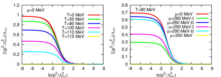
Figure 1: The mass functions $\Sigma(p)$ as functions of $p$. The left panel displays $\Sigma(p)$ with $\mu=0$ MeV at $T=0$, $50$, $80$, $100$, $110$ and $115$ MeV, respectively. The right panel displays $\Sigma(p)$ with $T=80$ MeV at $\mu=0$, $280$, $290$ and $300$ MeV, respectively.

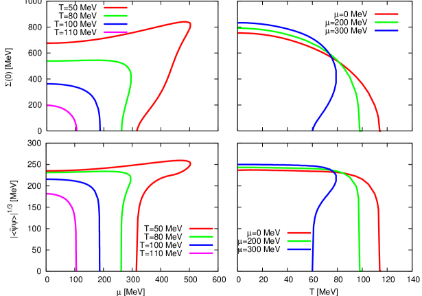
Figure 2: The chemical potential (left) and temperature (right) dependences of $\Sigma(0)$ and $|\langle\overline{\psi}\psi\rangle|^{1/3}$, respectively. The left figures plot these quantities at $T=50,80,100$ and $110$ MeV as functions of $\mu$. The right figures plot these two quantities at $\mu=0,200$ and $300$ MeV as functions of $T$.

3.2 Numerical results

We studied the case with two massless quark flavors ($i.e.$, $N_{f}=2$) and $N_{c}=3$, where $N_{c}$ is the number of colors. The model parameter $\Lambda_{\rm QCD}$ is fixed so as to reproduce the pion decay constant $f_{\pi}=93$ MeV in (13), and we obtain $\Lambda_{\rm QCD}\simeq 776$ MeV using the IR cutoff at $\ln(p_{IF}^{2}/\Lambda_{\rm QCD}^{2})=0.1$. Then, the quark condensate in the vacuum is found to be $|\langle\overline{\psi}\psi\rangle|^{1/3}\simeq 236$ MeV in this model, and it is insensitive to the value of the UV cutoff. (We use $\Lambda^{2}/\Lambda_{\rm QCD}^{2}=2.0\times 10^{4}$.)

At finite temperature and density, we numerically calculated the quark mass function $\Sigma(p)$ and the quark condensate $\langle\bar{\psi}\psi\rangle$. In Fig. 1 we plot the mass function $\Sigma(p)$. The left panel displays $\Sigma(p)$ with $\mu=0$ MeV at $T=0$, $50$, 80, $100$, $110$ and $115$ MeV, respectively, while the right panel displays $\Sigma(p)$ with fixed $T=80$ MeV at $\mu=0$, $280$, $290$ and $300$ MeV, respectively. At the finite chemical potentials $\mu=280$ and $290$ MeV with $T=80$ MeV, there exist two non-trivial solutions for $\Sigma(p)$, which we denote I and II. The free energy of the solution I is lower than that of II.

In the left panels of Fig. 2, we plot the $\mu$ dependences of $\Sigma(0)$ and $\langle\overline{\psi}\psi\rangle$, respectively, at $T=50,80,100$ and $110$ MeV. The right panels present the $T$ dependences of the same quantities at $\mu=0,200$ and $300$ MeV. In the region of low temperature and large chemical potential, we find two non-trivial extremum solutions, $\Sigma\neq 0$, in addition to the trivial one, which indicates a first-order transition. It should be noted here that the chiral condensate $\langle{\bar{\psi}}\psi\rangle$ and the value of $\Sigma(0)$ increase as $\mu$ increases in the case of fixed $T=50$ MeV, as is seen in Fig. 2. This behavior is known to be an artifact of the approximation made by omitting $\Sigma_{s}$ and $\Sigma_{v}$. If $\Sigma_{s}$ and $\Sigma_{v}$ are properly taken into account, $\langle{\bar{\psi}}\psi\rangle$ and $\Sigma(0)$ are found to decrease monotonically, and the chiral symmetry is restored, as $\mu$ increases.[20]

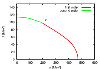
Figure 3: The phase diagram for the chiral symmetry. The transition point is located at $T_{c}\simeq 114$ MeV for $\mu=0$ MeV, $\mu_{c}\simeq 472$ MeV at $T=0$ MeV, and so on. The tri-critical point $P$ is located at $(T_{t},\mu_{t})\simeq(97,203)$ MeV.

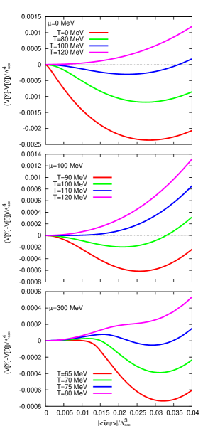
Figure 4: The temperature and chemical potential dependence of the effective potential, $V[\Sigma_{c},J]-V[0]$, with fixed $\mu$ as a function of $|\langle{\bar{\psi}}\psi\rangle|$.

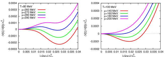
Figure 5: The temperature and chemical potential dependence of the effective potential, $V[\Sigma_{c},J]-V[0]$, with fixed $T$ as a function of $|\langle{\bar{\psi}}\psi\rangle|$.

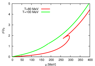
Figure 6: The chemical potential dependence of the quark number density at $T=80$ and $100$ MeV. Here, $\rho_{0}=3\times 0.17\ {\textrm{fm}^{-3}}$.

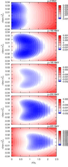
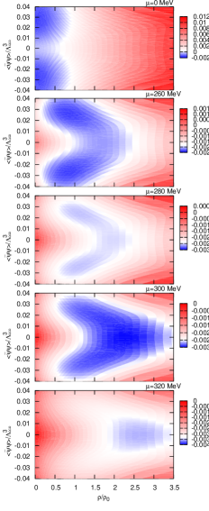
Figure 7: The contour map for $\overline{V}(\langle{\bar{\psi}}\psi\rangle,\rho\ ;\mu,T)$ in the $\rho$-$\langle{\bar{\psi}}\psi\rangle$ plane with various chemical potentials for $T=100$ MeV (left) and $T=80$ MeV (right).

We present the phase diagram of the model in Fig.3, where the tri-critical point appears at $(T_{t},\mu_{t})\simeq(97,203)$ MeV.

The situation may be more clearly understood if we can obtain the explicit functional form of the effective potential. We plot $V[\Sigma_{c}]-V[0]$ as a function of $|\langle{\overline{\psi}}\psi\rangle|/\Lambda_{\rm QCD}^{3}$ in Fig. 4 at $\mu=0$, 100 and 300 MeV for several values of $T$. In Fig. 5 we plot the results at $T=80$ and 100 MeV with several values of $\mu$. As seen from the behavior of the effective potential in Fig. 4, a second-order transition occurs in the range $T=$ 100 – 120 MeV in the cases with $\mu=0$ and $\mu=100$ MeV. At $\mu=300$ MeV, however, a first-order transition occurs between $T=75$ MeV and 80 MeV. Similarly, in Fig. 5, a first-order transition is seen to occur when the chemical potential is changed between $\mu=280$ MeV and 290 MeV at low temperature ($T=80$ MeV), while the transition is second order at fixed $T=100$ MeV. In Fig. 6, the quark number density $\rho$ is plotted in units of the normal nuclear matter density in terms of quark numbers, $\rho_{0}=3\times 0.17\ {\rm fm}^{-3}$, as a function of $\mu$ with fixed $T=80$ MeV and 100 MeV. The transition points are $\mu=282$ MeV at $T=80$ MeV and $\mu=187$ MeV at $T=100$ MeV. In the former case, the quark number density has a gap. In the latter, it is continuous but its derivative (the susceptibility) has a gap.

In Fig. 7, we plot the contour map of the Landau potential ${\overline{V}}(\langle{\bar{\psi}}\psi\rangle,\rho;\mu,T)$ given in (27) as a function of the quark condensate and the quark number density at several values of $\mu$ with fixed $T$. Note that a tri-critical point is located at $(T_{t},\mu_{t})\simeq(97,203)$ MeV. The vertical axis represents $\langle{\bar{\psi}}\psi\rangle/\Lambda_{\rm QCD}^{3}$, and the horizontal axis represents the quark number density in units of $\rho_{0}$. We plot the contour map at $T=100$ MeV, where a second-order transition occurs, in the left panels of Fig.7. At $\mu=0$, the two minima are positioned symmetrically in the $\rho$-$\langle{\bar{\psi}}\psi\rangle$ plane at $\rho=0$ with finite values of the quark condensate, $\langle{\bar{\psi}}\psi\rangle$. As the chemical potential increases, the two minima approach each other for finite $\rho$, and then fuse continuously to form a single minimum at $\langle{\bar{\psi}}\psi\rangle=0$ and finite $\rho$.

The contour map for $T=80$ MeV is plotted in the right panels of Fig.7. At $\mu=0$, the two minima are positioned symmetrically in the $\rho$–$\langle{\bar{\psi}}\psi\rangle$ plane at $\rho=0$ and finite values of the quark condensate, $\langle{\bar{\psi}}\psi\rangle$, just as in the $T=100$ MeV case. By contrast, however, one new local minimum appears at $\langle{\bar{\psi}}\psi\rangle=0$ as $\mu$ increases, and three local minima exist in a certain range of $\mu$. At the critical point, these three minima are energetically degenerate, and we observe a first-order chiral phase transition.

4 Summary

We have analyzed the chiral phase transition of a QCD-like theory at finite temperature and density using the effective potential. We have devised a method to derive an effective potential in order to elucidate the global behavior of the phase transition. There we introduced a bilocal external source field and solved the Schwinger-Dyson equation with this source field. This solution of the SD equation gives the extremum of the effective potential with the source field. Then, subtracting the interaction energy with the source we obtained the original effective potential for this configuration. In this way we showed the shape of the effective potential of the QCD-like theory at finite temperature, $T$, and quark chemical potential, $\mu$. From the temperature dependence of the effective potential, we have a second-order phase transition along the $\mu=0$ line. Contrastingly, we have a first-order phase transition along the $T=0$ line. Also, we have introduced the Landau potential and plotted its contour map with respect to the quark condensate and the quark number density. We conclude that our method to construct the effective potential of the QCD-like theory is very useful for understanding the features of the chiral phase transition of the model.

Appendix A Calculation of the Effective Potential in the NJL Model

For pedagogical reasons, here we apply our method with a source field coupled quadratically to the auxiliary field, to the Nambu-Jona-Lasinio (NJL) model, whose Lagrangian density takes the form

$$\mathcal{L}=\overline{\psi}i\raise 0.6458pt\hbox{$/$}\kern-5.29999pt\hbox{$\partial$}\psi+\frac{\lambda}{2N}\left((\overline{\psi}\psi)^{2}+(\overline{\psi}i\gamma_{5}{\boldmath\tau}\psi)^{2}\right).$$ (28)

We introduce the auxiliary field into the scalar part of the 4-fermi interaction and ignore the pseudo-scalar part for the moment, as we know that the potential is chirally symmetric. To leading order in the $1/N$ expansion, we obtain the effective potential at finite $T$ and $\mu$ as

$$V(T,\mu,\chi) = \!\!\frac{\chi^{2}}{2\lambda}-2N_{c}N_{f}T\!\sum^{\infty}_{n=-\infty}\!\int\frac{d^{3}\mib{k}}{(2\pi)^{3}}\textrm{ln}[(\omega_{n}-i\mu)^{2}+\mib{k}^{2}+\chi^{2}]$$ (29)

$$= \frac{\chi^{2}}{2\lambda}-\frac{N_{c}N_{f}}{2\pi^{2}}\int^{\chi^{2}}_{0}dx\int^{\Lambda}_{0}d|\mib{k}|\frac{\mib{k}^{2}}{\sqrt{\mib{k}^{2}+x}}(1-n_{+}(x)-n_{-}(x)),$$

where $\chi=-\lambda\overline{\psi}\psi/N$ is an auxiliary field, and $n_{\pm}(x)=[\exp(\sqrt{\mib{k}^{2}+x}\mp\mu)+1]^{-1}$.

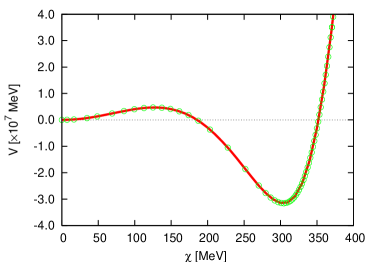
Figure 8: Two effective potentials $V(\chi)-V(\chi=0)$ (solid curve) and ${V}(\chi,J)-V(\chi=0,J=0)$ (round points) composed in the case $T=10$ MeV and $\mu=320$ MeV.

The functional form of the potential is easily obtained through the numerical integration of Eq. (29). To demonstrate our method, we consider the case of a constant source coupled to the field $\chi^{2}$:[33]

$$\widetilde{V}(\chi,J)=V(\chi)+\frac{1}{2}J\chi^{2}.$$ (30)

Rewriting the source $J$ as $J=c\lambda^{-1}$, we obtain

$$\widetilde{V}(\chi,J) = (1+c)\frac{\chi^{2}}{2\lambda}-\frac{N_{c}N_{f}}{2\pi^{2}}\int^{\chi^{2}}_{0}\!\!dx\int^{\Lambda}_{0}\!d|\mib{k}|\frac{\mib{k}^{2}}{\sqrt{\mib{k}^{2}+x}}(1-n_{+}(x)-n_{-}(x)),\qquad$$ (31)

and the corresponding SD equation, $\partial\widetilde{V}/\partial\chi=0$:

$$\frac{\chi_{c}}{\lambda} = \frac{1}{1+c}\frac{N_{c}N_{f}\chi_{c}}{\pi^{2}}\int^{\Lambda}_{0}d|\mib{k}|\frac{\mib{k}^{2}}{\sqrt{\mib{k}^{2}+\chi_{c}^{2}}}(1-n_{+}(\chi_{c}^{2})-n_{-}(\chi_{c}^{2})).$$ (32)

The value of the effective potential at $\chi=\chi_{c}$ is obtained from $\tilde{V}_{\rm ex}(\chi_{c})$ using the Legendre transformation:

$$\bar{V}(\chi_{c})=\tilde{V}_{\rm ex}(\chi_{c})-\frac{1}{2}J\chi_{c}^{2}\ .$$ (33)

In the stationary-phase approximation for $\chi$, we should have the trivial result

$$V(\chi)=\bar{V}(\chi).$$ (34)

One of the advantages of the source (30) is that it allows us to probe the non-convex effective potential near a second-order transition. Near a first-order transition point, the SD equation (32) has two non-trivial solutions for a certain range of $c$. We need both the solutions in order to re-construct the full shape of the potential via Eq. (33).

We present the result in the massless two-flavor case ($N_{c}=3$ and $N_{f}=2$) here. We fixed the three-momentum cutoff as $\Lambda\simeq 653$ MeV and the coupling constant as $\lambda\Lambda^{2}\simeq 4.29$ with the constituent quark mass $313$ MeV and $f_{\pi}=93$ MeV. In Fig.8, we compare the effective potential $\bar{V}(\chi)$ (circles), constructed using the applied source and the Legendre transformation, with the original $V(\chi)$ (solid curve). It is seen that they are essentially coincident, as should be the case. Hence, we conclude that our method successfully reproduces the potential in the non-convex region[33].

References

- [1] J. C. Collins and M. J. Perry, Phys. Rev. Lett. 34 (1975), 1353.
- [2] See, for example, Quark-Gluon Plasma 3, ed. R. C. Hwa and X.-N. Wang (World Scientific, Singapore, 2004).
- [3] See, for example, T. Kunihiro, T. Muto, T. Takatsuka, R. Tamagaki and T. Tatsumi, Prog. Theor. Phys. Suppl. No. 112 (1993).
- [4] See, for example, Prog. Theor. Phys. Suppl. No. 153 (2004).
-
[5]
T. Hatsuda and T. Kunihiro, Phys. Rep. 247 (1994), 1.
S. P. Klevansky, Rev. Mod. Phys. 63 (1992), 649. - [6] M. Asakawa and K. Yazaki, Nucl. Phys. A 504 (1989), 668.
- [7] A. Barducci, R. Casalbuoni, S. De Curtis, R. Gatto and G. Pettini, Phys. Lett. B 231 (1989), 463.
- [8] A Barducci, R. Casalbuoni, G. Pettini and R. Gatto, Phys. Rev. D 49 (1994), 426; ibid. 41 (1990), 1610.
- [9] D. Bailin and A. Love, Phys. Rep. 107 (1984), 325.
- [10] M. Iwasaki and T. Iwado, Phys. Lett. 350 (1995), 163; Prog. Theor. Phys. 94 (1995), 1073.
- [11] M. Alford, K. Rajagopal and F. Wilczek, Phys. Lett. B 422 (1998), 247.
- [12] R. Rapp, T. Schäfer, E. V. Shuryak and M. Velkovsky, Phys. Rev. Lett. 81 (1998), 53.
- [13] K.-I. Aoki, M. Bando, T. Kugo, M. G. Mitchard and H. Nakatani, Prog. Theor. Phys. 84 (1990), 683.
- [14] T. Kugo, Dynamical Symmetry Breaking, ed. by K. Yamawaki (World Scientific, Singapore, 1992), p.35.
- [15] K. Higashijima, Prog. Theor. Phys. Suppl. No. 104 (1991), 1.
- [16] H. Fujii and Y. Tsue, Phys. Lett. B 357 (1995), 199.
- [17] Y. Taniguchi and Y. Yoshida, Phys. Rev. D 55 (1997), 2283.
- [18] M. Harada and A. Shibata, Phys. Rev. D 59 (1998), 014010.
- [19] O. Kiriyama, M. Maruyama and F. Takagi, Phys. Rev. D 62 (2000), 105008.
- [20] T. Ikeda, Prog. Theor. Phys. 107 (2002), 403.
- [21] S. Takagi, Prog. Theor. Phys. 109 (2003), 233.
- [22] H. Abuki, Prog. Theor. Phys. 110 (2003), 937.
- [23] J. M. Cornwall, R. Jackiw and E. Tomboulis, Phys. Rev. D 10 (1974), 2428.
- [24] R. W. Haymaker, Riv. Nuovo. Cim. 14 (1991), 1.
-
[25]
K. Higashijima, Phys. Rev. D 29 (1984), 1228.
V. A. Miransky, Sov. J. Nucl. Phys. 38 (1983), 280. - [26] S. Sasaki, H. Suganuma and H. Toki, Phys. Lett. B 387 (1996), 145.
- [27] T. Maskawa and H. Nakajima, Prog. Theor. Phys. 52 (1974), 1326.
- [28] H. Pagels and S. Stokar, Phys. Rev. D 20 (1979), 11.
- [29] O. Kaczmarek, F. Karsch, F. Zantow and P. Petreczky, Phys. Rev. D 70 (2004), 074505.
- [30] T. Morozumi and H. So, Prog. Theor. Phys. 77 (1987), 1434.
- [31] H. Fujii and M. Ohtani, Phys. Rev. D 70 (2004), 014016.
- [32] N. Goldenfeld, Lectures on Phase Transitions and the Renormalization Group (Addison-Wesley Pub. Co., 1992).
- [33] H. Ichie, H. Suganuma and H. Toki, Phys. Rev. D 52 (1995), 2944.