Preface

The present text is based on lectures given in the context of the ECT^∗ Doctoral Training Programme 2005 (Marie Curie Training Site) Hadronic Physics at the European Centre for Theoretical Studies in Nuclear Physics and Related Areas (ECT^∗) in Trento, Italy.

The course was addressed to PhD students with both rather different interests and background in experimental and theoretical nuclear and particle physics. The students were assumed to be familiar with elementary concepts of field theory and relativistic quantum mechanics. The goal of the course was to provide a pedagogical introduction to the basic concepts of chiral perturbation theory (ChPT) in the mesonic and baryonic sectors. We have tried to also work out those pieces which by the “experts” are considered as well known. In particular, we have often included intermediate steps in derivations in order to facilitate the understanding of the origin of the final results. We have tried to keep a reasonable balance between mathematical rigor and illustrations by means of simple examples. Some of the topics not directly related to ChPT were covered in extra lectures in the afternoon. By preparing numerous exercises, covering a wide range of difficulty—from very easy to quite difficult—, we hoped to take the different individual levels of experience into account. Ideally, at the end of the course, a participant (or a reader of these notes) should be able to perform simple calculations in the framework of ChPT and to read the current literature.

These lecture notes include the following topics. Chapter 1 deals with QCD and its global symmetries in the chiral limit, explicit symmetry breaking in terms of the quark masses, and the concept of Green functions and Ward identities reflecting the underlying chiral symmetry. In Chapter 2 the idea of a spontaneous breakdown of a global symmetry is discussed and its consequences in terms of the Goldstone theorem are demonstrated. Chapter 3 deals with mesonic chiral perturbation theory and the principles entering the construction of the chiral Lagrangian are outlined. In Chapter 4 the methods are extended to include the interaction between Goldstone bosons and baryons in the single-baryon sector. Sections marked with an asterisk may be omitted in a first reading.

Mainz and Trento, May 2005

Stefan Scherer and Matthias R. Schindler

Readers interested in the present status of applications are referred to lecture notes and review articles [Leutwyler:pf:1991mz, Bijnens:pf:xi, Meissner:pf:1993ah, Leutwyler:pf:1994fi, Bernard:pf:1995dp, deRafael:pf:1995zv, Pich:pf:1995bw, Ecker:pf:1995gg, Manohar:pf:1996cq, Pich:pf:1998xt, Burgess:pf:1998ku, Scherer:pf:2002tk] as well as conference proceedings [Bernstein:pf:zq, Bernstein:pf:pm, Bernstein:pf:2002, Meissner:pf:2003hr].

Acknowledgements

The authors would like to thank the co-ordinator Matthias F. M. Lutz and the co-organizers Michael Birse and W. Vogelsang for the invitation to participate in the program. Moreover, we would like to thank Prof. J. - P. Blaizot, Prof. G. Ripka, Stefania Campregher, and Donatella Rosetti for the hospitality and the pleasant working conditions at ECT^∗. M. R. S. acknowledges the support through a Marie Curie fellowship. S. S. would like to thank the participants for their enthusiasm, staying power, and patience to survive 24 lectures in one week.

Chapter 1 QCD and Chiral Symmetry

1.1 Some Remarks on SU(3)

The group SU(3) plays an important role in the context of the strong interactions, because

1. it is the gauge group of quantum chromodynamics (QCD);

2. flavor SU(3) is approximately realized as a global symmetry of the hadron spectrum, so that the observed (low-mass) hadrons can be organized in approximately degenerate multiplets fitting the dimensionalities of irreducible representations of SU(3);

3. the direct product $\mbox{SU(3)}_{L}\times\mbox{SU(3)}_{R}$ is the chiral-symmetry group of QCD for vanishing $u$-, $d$-, and $s$-quark masses.

Thus, it is appropriate to first recall a few basic properties of SU(3) and its Lie algebra su(3).

The group SU(3) is defined as the set of all unitary, unimodular, $3\times 3$ matrices $U$, i.e. $U^{\dagger}U=1$, and $\mbox{det}(U)=1$. In mathematical terms, SU(3) is an eight-parameter, simply connected, compact Lie group. This implies that any group element can be parameterized by a set of eight independent real parameters $\Theta=(\Theta_{1},\cdots,\Theta_{8})$ varying over a continuous range. The Lie-group property refers to the fact that the group multiplication of two elements $U(\Theta)$ and $U(\Psi)$ is expressed in terms of eight analytic functions $\Phi_{i}(\Theta;\Psi)$, i.e. $U(\Theta)U(\Psi)=U(\Phi)$, where $\Phi=\Phi(\Theta;\Psi)$. It is simply connected because every element can be connected to the identity by a continuous path in the parameter space and compactness requires the parameters to be confined in a finite volume. Finally, for compact Lie groups, every finite-dimensional representation is equivalent to a unitary one and can be decomposed into a direct sum of irreducible representations (Clebsch-Gordan series).

Elements of SU(3) are conveniently written in terms of the exponential representation

$$U(\Theta)=\exp\left(-i\sum_{a=1}^{8}\Theta_{a}\frac{\lambda_{a}}{2}\right),$$ (1.1)

with $\Theta_{a}$ real numbers, and where the eight linearly independent matrices $\lambda_{a}$ are the so-called Gell-Mann matrices, satisfying

$$\frac{\lambda_{a}}{2} = i\frac{\partial U}{\partial\Theta_{a}}(0,\cdots,0),$$ (1.2)

$$\lambda_{a} = \lambda_{a}^{\dagger},$$ (1.3)

$$\mbox{Tr}(\lambda_{a}\lambda_{b}) = 2\delta_{ab},$$ (1.4)

$$\mbox{Tr}(\lambda_{a}) = 0.$$ (1.5)

The Hermiticity of Eq. (1.3) is responsible for $U^{\dagger}=U^{-1}$. On the other hand, since $\mbox{det}[\exp(C)]=\exp[\mbox{Tr}(C)]$, Eq. (1.5) results in $\mbox{det}(U)=1$. An explicit representation of the Gell-Mann matrices is given by

$$\lambda_{1}=\left(\begin{array}[]{rrr}0&1&0\\ 1&0&0\\ 0&0&0\end{array}\right),\quad\lambda_{2}=\left(\begin{array}[]{rrr}0&-i&0\\ i&0&0\\ 0&0&0\end{array}\right),\quad\lambda_{3}=\left(\begin{array}[]{rrr}1&0&0\\ 0&-1&0\\ 0&0&0\end{array}\right),$$ (1.15)

$$\lambda_{4}=\left(\begin{array}[]{rrr}0&0&1\\ 0&0&0\\ 1&0&0\end{array}\right),\quad\lambda_{5}=\left(\begin{array}[]{rrr}0&0&-i\\ 0&0&0\\ i&0&0\end{array}\right),\quad\lambda_{6}=\left(\begin{array}[]{rrr}0&0&0\\ 0&0&1\\ 0&1&0\end{array}\right),$$ (1.25)

$$\lambda_{7}=\left(\begin{array}[]{rrr}0&0&0\\ 0&0&-i\\ 0&i&0\end{array}\right),\quad\lambda_{8}=\sqrt{\frac{1}{3}}\left(\begin{array}[]{rrr}1&0&0\\ 0&1&0\\ 0&0&-2\end{array}\right).$$ (1.32)

The set $\{i\lambda_{a}\}$ constitutes a basis of the Lie algebra su(3) of SU(3), i.e., the set of all complex, traceless, skew-Hermitian, $3\times 3$ matrices. The Lie product is then defined in terms of ordinary matrix multiplication as the commutator of two elements of su(3). Such a definition naturally satisfies the Lie properties of anti-commutativity

$$[A,B]=-[B,A]$$ (1.33)

as well as the Jacobi identity

$$[A,[B,C]]+[B,[C,A]]+[C,[A,B]]=0.$$ (1.34)

In accordance with Eqs. (1.1) and (1.2), elements of su(3) can be interpreted as tangent vectors in the identity of SU(3).

The structure of the Lie group is encoded in the commutation relations of the Gell-Mann matrices,

$$\left[\frac{\lambda_{a}}{2},\frac{\lambda_{b}}{2}\right]=if_{abc}\frac{\lambda_{c}}{2},$$ (1.35)

where the totally antisymmetric real structure constants $f_{abc}$ are obtained from Eq. (1.4) as

$$f_{abc}=\frac{1}{4i}\mbox{Tr}([\lambda_{a},\lambda_{b}]\lambda_{c}).$$ (1.36)

Exercise 1.1.1

Verify Eq. (1.36).

Hint: Multipy Eq. (1.35) by $\lambda_{d}$, take the trace, make use of Eq. (1.4), and finally rename $d\to c$.

Exercise 1.1.2

Show that $f_{abc}$ is totally antisymmetric.

Hint: Consider the symmetry properties of $\mbox{Tr}([A,B]C)$.

The independent non-vanishing values are explicitly summarized in the scheme of Table 1.1. Roughly speaking, these structure constants are a measure of the non-commutativity of the group SU(3).

$abc$	123	147	156	246	257	345	367	458	678
$f_{abc}$	1	$\frac{1}{2}$	$-\frac{1}{2}$	$\frac{1}{2}$	$\frac{1}{2}$	$\frac{1}{2}$	$-\frac{1}{2}$	$\frac{1}{2}\sqrt{3}$	$\frac{1}{2}\sqrt{3}$

Table 1.1: Totally antisymmetric non-vanishing structure constants of SU(3).

The anti-commutation relations of the Gell-Mann matrices read

$$\{\lambda_{a},\lambda_{b}\}=\frac{4}{3}\delta_{ab}+2d_{abc}\lambda_{c},$$ (1.37)

where the totally symmetric $d_{abc}$ are given by

$$d_{abc}=\frac{1}{4}\mbox{Tr}(\{\lambda_{a},\lambda_{b}\}\lambda_{c}),$$ (1.38)

and are summarized in Table 1.2.

Exercise 1.1.3

Verify Eq. (1.38) and show that $d_{abc}$ is totally symmetric.

Clearly, the anti-commutator of two Gell-Mann matrices is not necessarily a Gell-Mann matrix. For example, the square of a (nontrivial) skew-Hermitian matrix is not skew Hermitian.

$abc$	118	146	157	228	247	256	338	344
$d_{abc}$	$\frac{1}{\sqrt{3}}$	$\frac{1}{2}$	$\frac{1}{2}$	$\frac{1}{\sqrt{3}}$	$-\frac{1}{2}$	$\frac{1}{2}$	$\frac{1}{\sqrt{3}}$	$\frac{1}{2}$
$abc$	355	366	377	448	558	668	778	888
$d_{abc}$	$\frac{1}{2}$	$-\frac{1}{2}$	$-\frac{1}{2}$	$-\frac{1}{2\sqrt{3}}$	$-\frac{1}{2\sqrt{3}}$	$-\frac{1}{2\sqrt{3}}$	$-\frac{1}{2\sqrt{3}}$	$-\frac{1}{\sqrt{3}}$

Table 1.2: Totally symmetric non-vanishing $d$ symbols of SU(3).

Moreover, it is convenient to introduce as a ninth matrix

$$\lambda_{0}=\sqrt{2/3}\,\mbox{diag}(1,1,1),$$

such that Eqs. (1.3) and (1.4) are still satisfied by the nine matrices $\lambda_{a}$. In particular, the set $\{i\lambda_{a}|a=0,\cdots,8\}$ constitutes a basis of the Lie algebra u(3) of U(3), i.e., the set of all complex, skew-Hermitian, $3\times 3$ matrices.

• Many useful properties of the Gell-Mann matrices can be found in Sect. 8 of CORE (Compendium of relations) by V. I. Borodulin, R. N. Rogalyov, and S. R. Slabospitsky, arXiv:hep-ph/9507456.

Finally, an arbitrary $3\times 3$ matrix $M$ can be written as

$$M=\sum_{a=0}^{8}\lambda_{a}M_{a},$$ (1.39)

where $M_{a}$ are complex numbers given by

$$M_{a}=\frac{1}{2}\mbox{Tr}(\lambda_{a}M).$$

1.2 The QCD Lagrangian

QCD is the gauge theory of the strong interactions [Gross:1973id:2, Weinberg:un:2, Fritzsch:pi:2] with color SU(3) as the underlying gauge group. The matter fields of QCD are the so-called quarks which are spin-1/2 fermions, with six different flavors in addition to their three possible colors (see Table 1.3). Since quarks have not been observed as asymptotically free states, the meaning of quark masses and their numerical values are tightly connected with the method by which they are extracted from hadronic properties (see Ref. [Manohar_PDG:2] for a thorough discussion).

flavor	u	d	s
charge [e]	$2/3$	$-1/3$	$-1/3$
mass [MeV]	$5.1\pm 0.9$	$9.3\pm 1.4$	$175\pm 25$
flavor	c	b	t
charge [e]	$2/3$	$-1/3$	$2/3$
mass [GeV]	$1.15-1.35$	$4.0-4.4$	$174.3\pm 3.2\pm 4.0$

Table 1.3: Quark flavors and their charges and masses. The absolute magnitude of $m_{s}$ is determined using QCD sum rules. The result is given for the $\overline{\mbox{MS}}$ running mass at scale $\mu=1$  GeV. The light quark masses are obtained from the mass ratios found using chiral perturbation theory, using the strange quark mass as input. The heavy-quark masses $m_{c}$ and $m_{b}$ are determined by the charmonium and D masses, and the bottomium and B masses, respectively. The top quark mass $m_{t}$ results from the measurement of lepton + jets and dilepton + jets channels in the D$\emptyset$ and CDF experiments at Fermilab.

The QCD Lagrangian can be obtained from the Lagrangian for free quarks by applying the gauge principle with respect to the group SU(3). It reads

$${\cal L}_{\rm QCD}=\sum_{f={u,d,s,\atop c,b,t}}\bar{q}_{f}(iD/-m_{f})q_{f}-\frac{1}{4}{\cal G}_{\mu\nu,a}{\cal G}^{\mu\nu}_{a}.$$ (1.40)

For each quark flavor $f$ the quark field $q_{f}$ consists of a color triplet (subscripts $r$, $g$, and $b$ standing for “red,” “green,” and “blue”),

$$q_{f}=\left(\begin{array}[]{c}q_{f,r}\\ q_{f,g}\\ q_{f,b}\end{array}\right),$$ (1.41)

which transforms under a gauge transformation $g(x)$ described by the set of parameters $\Theta(x)=[\Theta_{1}(x),\cdots,\Theta_{8}(x)]$ according to

$$q_{f}\mapsto q_{f}^{\prime}=\exp\left[-i\sum_{a=1}^{8}\Theta_{a}(x)\frac{\lambda_{a}^{C}}{2}\right]q_{f}=U[g(x)]q_{f}.$$ (1.42)

Technically speaking, each quark field $q_{f}$ transforms according to the fundamental representation of color SU(3). Because SU(3) is an eight-parameter group, the covariant derivative of Eq. (1.40) contains eight independent gauge potentials ${\cal A}_{\mu,a}$,

$$D_{\mu}\left(\begin{array}[]{l}q_{f,r}\\ q_{f,g}\\ q_{f,b}\end{array}\right)=\partial_{\mu}\left(\begin{array}[]{l}q_{f,r}\\ q_{f,g}\\ q_{f,b}\end{array}\right)-ig\sum_{a=1}^{8}\frac{\lambda_{a}^{C}}{2}{\cal A}_{\mu,a}\left(\begin{array}[]{l}q_{f,r}\\ q_{f,g}\\ q_{f,b}\end{array}\right).$$ (1.43)

We note that the interaction between quarks and gluons is independent of the quark flavors which can be seen from the fact that there only appears one coupling constant $g$ in Eq. (1.43). Demanding gauge invariance of ${\cal L}_{\rm QCD}$ imposes the following transformation property of the gauge fields (summation over $a$ implied)

$${\cal A}_{\mu}\equiv\frac{\lambda_{a}^{C}}{2}{\cal A}_{\mu,a}(x)\mapsto U[g(x)]{\cal A}_{\mu}(x)U^{\dagger}[g(x)]-\frac{i}{g}\partial_{\mu}U[g(x)]U^{\dagger}[g(x)].$$ (1.44)

Exercise 1.2.1

Show that the covariant derivative $D_{\mu}q_{f}$ transforms as $q_{f}$, i.e. $D_{\mu}q_{f}\mapsto D^{\prime}_{\mu}q^{\prime}_{f}=U(g)D_{\mu}q_{f}$.

Under a gauge transformation of the first kind, i.e., a global SU(3) transformation, the second term on the right-hand side of Eq. (1.44) would vanish and the gauge fields would transform according to the adjoint representation.

So far we have only considered the matter-field part of ${\cal L}_{\rm QCD}$ including its interaction with the gauge fields. Equation (1.40) also contains the generalization of the field strength tensor to the non-Abelian case,

$${\cal G}_{\mu\nu,a}=\partial_{\mu}{\cal A}_{\nu,a}-\partial_{\nu}{\cal A}_{\mu,a}+gf_{abc}{\cal A}_{\mu,b}{\cal A}_{\nu,c},$$ (1.45)

with the SU(3) structure constants given in Table 1.1 and a summation over repeated indices implied. Given Eq. (1.44) the field strength tensor transforms under SU(3) as

$${\cal G}_{\mu\nu}\equiv\frac{\lambda_{a}^{C}}{2}{\cal G}_{\mu\nu,a}\mapsto U[g(x)]{\cal G}_{\mu\nu}U^{\dagger}[g(x)].$$ (1.46)

Exercise 1.2.2

Verify Eq. (1.46).

Hint: Introduce ${\cal A}_{\mu}\equiv\lambda_{a}^{C}{\cal A}_{\mu,a}/2$. Equation (1.45) is then equivalent to ${\cal G}_{\mu\nu}=\partial_{\mu}{\cal A}_{\nu}-\partial_{\nu}{\cal A}_{\mu}-ig[{\cal A}_{\mu},{\cal A}_{\nu}]$.

Using Eq. (1.4) the purely gluonic part of ${\cal L}_{\rm QCD}$ can be written as

$$-\frac{1}{2}\mbox{Tr}_{C}({\cal G}_{\mu\nu}{\cal G}^{\mu\nu}),$$

which, using the cyclic property of traces, $\mbox{Tr}(AB)=\mbox{Tr}(BA)$, together with $UU^{\dagger}=1$, is easily seen to be invariant under the transformation of Eq. (1.46).

In contradistinction to the Abelian case of quantum electrodynamics, the squared field strength tensor gives rise to gauge-field self interactions involving vertices with three and four gauge fields of strength $g$ and $g^{2}$, respectively. Such interaction terms are characteristic of non-Abelian gauge theories and make them much more complicated than Abelian theories.

From the point of view of gauge invariance the strong-interaction Lagrangian could also involve a term of the type

$${\cal L}_{\theta}=\frac{g^{2}\bar{\theta}}{64\pi^{2}}\epsilon^{\mu\nu\rho\sigma}\sum_{a=1}^{8}{\cal G}^{a}_{\mu\nu}{\cal G}^{a}_{\rho\sigma},$$ (1.47)

where $\epsilon_{\mu\nu\rho\sigma}$ denotes the totally antisymmetric Levi-Civita tensor. The so-called $\theta$ term of Eq. (1.47) implies an explicit $P$ and $CP$ violation of the strong interactions which, for example, would give rise to an electric dipole moment of the neutron. The present empirical information indicates that the $\theta$ term is small and, in the following, we will omit Eq. (1.47) from our discussion.

1.3 Accidental, Global Symmetries of the QCD Lagrangian

1.3.1 Light and Heavy Quarks

The six quark flavors are commonly divided into the three light quarks $u$, $d$, and $s$ and the three heavy flavors $c$, $b$, and $t$,

$$\left(\begin{array}[]{r}m_{u}=0.005\,\mbox{GeV}\\ m_{d}=0.009\,\mbox{GeV}\\ m_{s}=0.175\,\mbox{GeV}\end{array}\right)\ll 1\,\mbox{GeV}\leq\left(\begin{array}[]{r}m_{c}=(1.15-1.35)\,\mbox{GeV}\\ m_{b}=(4.0-4.4)\,\mbox{GeV}\\ m_{t}=174\,\mbox{GeV}\end{array}\right),$$ (1.48)

where the scale of 1 GeV is associated with the masses of the lightest hadrons containing light quarks, e.g.,  $m_{\rho}$= 770 MeV, which are not Goldstone bosons resulting from spontaneous symmetry breaking. The scale associated with spontaneous symmetry breaking, $4\pi F_{\pi}\approx$ 1170 MeV, is of the same order of magnitude.

The masses of the lightest meson and baryon containing a charmed quark, $D^{+}=c\bar{d}$ and $\Lambda^{+}_{c}=udc$, are $(1869.4\pm 0.5)\,\mbox{MeV}$ and $(2284.9\pm 0.6)\,\mbox{MeV}$, respectively. The threshold center-of-mass energy to produce, say, a $D^{+}D^{-}$ pair in $e^{+}e^{-}$ collisions is approximately 3.74 GeV, and thus way beyond the low-energy regime which we are interested in. In the following, we will approximate the full QCD Lagrangian by its light-flavor version, i.e., we will ignore effects due to (virtual) heavy quark-antiquark pairs $h\bar{h}$.

Comparing the proton mass, $m_{p}$ = 938 MeV, with the sum of two up and one down current-quark masses (see Table 1.3),

$$m_{p}\gg 2m_{u}+m_{d},$$ (1.49)

shows that an interpretation of the proton mass in terms of current-quark mass parameters must be very different from, say, the situation in the hydrogen atom, where the mass is essentially given by the sum of the electron and proton masses, corrected by a small amount of binding energy. In this context we recall that the current-quark masses must not be confused with the constituent quark masses of a (nonrelativistic) quark model which are typically of the order of 350 MeV. In particular, Eq. (1.49) suggests that the Lagrangian ${\cal L}_{\rm QCD}^{0}$, containing only the light-flavor quarks in the so-called chiral limit $m_{u},m_{d},m_{s}\to 0$, might be a good starting point in the discussion of low-energy QCD:

$${\cal L}^{0}_{\rm QCD}=\sum_{l=u,d,s}\bar{q}_{l}iD/\hskip 3.00003ptq_{l}-\frac{1}{4}{\cal G}_{\mu\nu,a}{\cal G}^{\mu\nu}_{a}.$$ (1.50)

We repeat that the covariant derivative $D/\hskip 3.00003ptq_{l}$ acts on color and Dirac indices only, but is independent of flavor.

1.3.2 Left-Handed and Right-Handed Quark Fields

In order to fully exhibit the global symmetries of Eq. (1.50), we consider the chirality matrix $\gamma_{5}=\gamma^{5}=i\gamma^{0}\gamma^{1}\gamma^{2}\gamma^{3}=\gamma_{5}^{\dagger}$, $\{\gamma^{\mu},\gamma_{5}\}=0$, $\gamma_{5}^{2}=1$, and introduce projection operators

$$P_{R}=\frac{1}{2}(1+\gamma_{5})=P_{R}^{\dagger},\quad P_{L}=\frac{1}{2}(1-\gamma_{5})=P_{L}^{\dagger},$$ (1.51)

where the indices $R$ and $L$ refer to right-handed and left-handed, respectively, as will become more clear below. Obviously, the $4\times 4$ matrices $P_{R}$ and $P_{L}$ satisfy a completeness relation,

$$P_{R}+P_{L}=1,$$ (1.52)

are idempotent,

$$P_{R}^{2}=P_{R},\quad P_{L}^{2}=P_{L},$$ (1.53)

and respect the orthogonality relations

$$P_{R}P_{L}=P_{L}P_{R}=0.$$ (1.54)

Exercise 1.3.1

Verify the properties of Eqs. (1.51) – (1.54).

The combined properties of Eqs. (1.51) – (1.54) guarantee that $P_{R}$ and $P_{L}$ are indeed projection operators which project from the Dirac field variable $q$ to its chiral components $q_{R}$ and $q_{L}$,

$$q_{R}=P_{R}q,\quad q_{L}=P_{L}q.$$ (1.55)

We recall in this context that a chiral (field) variable is one which under parity is transformed into neither the original variable nor its negative. Under parity, the quark field is transformed into its parity conjugate,

$$P:q(t,\vec{x})\mapsto\gamma_{0}q(t,-\vec{x}),$$

and hence

$$q_{R}(t,\vec{x})=P_{R}q(t,\vec{x})\mapsto P_{R}\gamma_{0}q(t,-\vec{x})=\gamma_{0}q_{L}(t,-\vec{x})\neq\pm q_{R}(t,-\vec{x}),$$

and similarly for $q_{L}$.

The terminology right-handed and left-handed fields can easily be visualized in terms of the solution to the free Dirac equation. For that purpose, let us consider an extreme relativistic positive-energy solution to the free Dirac equation with three-momentum $\vec{p}$,

$$u(\vec{p},\pm)=\sqrt{E+m}\left(\begin{array}[]{c}\chi_{\pm}\\ \frac{\vec{\sigma}\cdot\vec{p}}{E+m}\chi_{\pm}\end{array}\right)\stackrel{{\scriptstyle\mbox{$E\gg m$}}}{{\mapsto}}\sqrt{E}\left(\begin{array}[]{r}\chi_{\pm}\\ \pm\chi_{\pm}\end{array}\right)\equiv u_{\pm}(\vec{p}\,),$$

where we assume that the spin in the rest frame is either parallel or antiparallel to the direction of momentum

$$\vec{\sigma}\cdot\hat{p}\chi_{\pm}=\pm\chi_{\pm}.$$

In the standard representation of Dirac matrices we find

$$P_{R}=\frac{1}{2}\left(\begin{array}[]{rr}1_{2\times 2}&1_{2\times 2}\\ 1_{2\times 2}&1_{2\times 2}\end{array}\right),\quad P_{L}=\frac{1}{2}\left(\begin{array}[]{rr}1_{2\times 2}&-1_{2\times 2}\\ -1_{2\times 2}&1_{2\times 2}\end{array}\right).$$

Exercise 1.3.2

Show that

$$P_{R}u_{+}=u_{+},\quad P_{L}u_{+}=0,\quad P_{R}u_{-}=0,\quad P_{L}u_{-}=u_{-}.$$

In the extreme relativistic limit (or better, in the zero-mass limit), the operators $P_{R}$ and $P_{L}$ project to the positive and negative helicity eigenstates, i.e., in this limit chirality equals helicity.

Our goal is to analyze the symmetry of the QCD Lagrangian with respect to independent global transformations of the left- and right-handed fields. There are 16 independent $4\times 4$ matrices, that can be expressed in terms of the unit matrix, the Dirac matrices $\gamma^{\mu}$, the chirality matrix $\gamma_{5}$, the products $\gamma^{\mu}\gamma_{5}$, and the six matrices $\sigma^{\mu\nu}=i[\gamma^{\mu},\gamma^{\nu}]/2$. In order to decompose the corresponding 16 quadratic forms into their respective projections to right- and left-handed fields, we make use of

$$\bar{q}\Gamma_{i}q=\left\{\begin{array}[]{lcl}\bar{q}_{R}\Gamma_{1}q_{R}+\bar{q}_{L}\Gamma_{1}q_{L}&\mbox{for}&\Gamma_{1}\in\{\gamma^{\mu},\gamma^{\mu}\gamma_{5}\}\\ \bar{q}_{R}\Gamma_{2}q_{L}+\bar{q}_{L}\Gamma_{2}q_{R}&\mbox{for}&\Gamma_{2}\in\{1,\gamma_{5},\sigma^{\mu\nu}\}\end{array}\right.,$$ (1.56)

where $\bar{q}_{R}=\bar{q}P_{L}$ and $\bar{q}_{L}=\bar{q}P_{R}.$

Exercise 1.3.3

Verify Eq. (1.56).

Hint: Insert unit matrices as

$$\bar{q}\Gamma_{i}q=\bar{q}(P_{R}+P_{L})\Gamma_{i}(P_{R}+P_{L})q,$$

and make use of $\{\Gamma_{1},\gamma_{5}\}=0$ and $[\Gamma_{2},\gamma_{5}]=0$ as well as the properties of the projection operators derived in Exercise 1.3.1.

We stress that the validity of Eq. (1.56) is general and does not refer to “massless” quark fields.

We now apply Eq. (1.56) to the term containing the contraction of the covariant derivative with $\gamma^{\mu}$. This quadratic quark form decouples into the sum of two terms which connect only left-handed with left-handed and right-handed with right-handed quark fields. The QCD Lagrangian in the chiral limit can then be written as

$${\cal L}^{0}_{\rm QCD}=\sum_{l=u,d,s}(\bar{q}_{R,l}iD/\hskip 3.00003ptq_{R,l}+\bar{q}_{L,l}iD/\hskip 3.00003ptq_{L,l})-\frac{1}{4}{\cal G}_{\mu\nu,a}{\cal G}^{\mu\nu}_{a}.$$ (1.57)

Due to the flavor independence of the covariant derivative ${\cal L}^{0}_{\rm QCD}$ is invariant under

$$\left(\begin{array}[]{c}u_{L}\\ d_{L}\\ s_{L}\end{array}\right)\mapsto U_{L}\left(\begin{array}[]{c}u_{L}\\ d_{L}\\ s_{L}\end{array}\right)=\exp\left(-i\sum_{a=1}^{8}\Theta^{L}_{a}\frac{\lambda_{a}}{2}\right)e^{-i\Theta^{L}}\left(\begin{array}[]{c}u_{L}\\ d_{L}\\ s_{L}\end{array}\right),$$ (1.67)

$$\left(\begin{array}[]{c}u_{R}\\ d_{R}\\ s_{R}\end{array}\right)\mapsto U_{R}\left(\begin{array}[]{c}u_{R}\\ d_{R}\\ s_{R}\end{array}\right)=\exp\left(-i\sum_{a=1}^{8}\Theta^{R}_{a}\frac{\lambda_{a}}{2}\right)e^{-i\Theta^{R}}\left(\begin{array}[]{c}u_{R}\\ d_{R}\\ s_{R}\end{array}\right),$$ (1.77)

where $U_{L}$ and $U_{R}$ are independent unitary $3\times 3$ matrices and where we have extracted the factors $e^{-i\Theta^{L}}$ and $e^{-i\Theta^{R}}$ for future convenience. Note that the Gell-Mann matrices act in flavor space.

${\cal L}^{0}_{\rm QCD}$ is said to have a classical global $\mbox{U(3)}_{L}\times\mbox{U(3)}_{R}$ symmetry. Applying Noether’s theorem from such an invariance one would expect a total of $2\times(8+1)=18$ conserved currents.

1.3.3 Noether Theorem

Noether’s theorem establishes the connection between continuous symmetries of a dynamical system and conserved quantities (constants of the motion). For simplicity we consider only internal symmetries. (The method can also be used to discuss the consequences of Poincaré invariance.)

In order to identify the conserved currents associated with the transformations of Eqs. (1.67), we briefly recall the method of Gell-Mann and Lévy [Gell-Mann:1960np:3:3], which we will then apply to Eq. (1.57).

We start with a Lagrangian ${\cal L}$ depending on $n$ independent fields $\Phi_{i}$ [typically $n\geq 2$ for bosons, and $n\geq 1$ for fermions, e.g. U(1)] and their first partial derivatives (the extension to higher-order derivatives is also possible),

$${\cal L}={\cal L}(\Phi_{i},\partial_{\mu}\Phi_{i}),$$ (1.78)

from which one obtains $n$ equations of motion:

$$\frac{\partial\cal L}{\partial\Phi_{i}}-\partial_{\mu}\frac{\partial\cal L}{\partial\partial_{\mu}\Phi_{i}}=0,\quad i=1,\cdots,n.$$ (1.79)

Suppose the Lagrangian of Eq. (1.78) to be invariant under a global symmetry transformation depending on $r$ real parameters. The method of Gell-Mann and Lévy now consists of promoting this global symmetry to a local one, from which we will then be able to identify the Noether currents. To that end we consider transformations which depend on $r$ real local parameters $\epsilon_{a}(x)$,

$$\Phi_{i}(x)\mapsto\Phi^{\prime}_{i}(x)=\Phi_{i}(x)+\delta\Phi_{i}(x)=\Phi_{i}(x)-i\epsilon_{a}(x)F^{a}_{i}[\Phi_{j}(x)],$$ (1.80)

and obtain, neglecting terms of order $\epsilon^{2}$, as the variation of the Lagrangian,

$$\delta{\cal L} = {\cal L}(\Phi^{\prime}_{i},\partial_{\mu}\Phi^{\prime}_{i})-{\cal L}(\Phi_{i},\partial_{\mu}\Phi_{i})$$ (1.81)

$$= \frac{\partial\cal L}{\partial\Phi_{i}}\delta\Phi_{i}+\frac{\partial\cal L}{\partial\partial_{\mu}\Phi_{i}}\underbrace{\partial_{\mu}\delta\Phi_{i}}_{\mbox{$-i[\partial_{\mu}\epsilon_{a}(x)]F^{a}_{i}-i\epsilon_{a}(x)\partial_{\mu}F^{a}_{i}$}}$$

$$= \epsilon_{a}(x)\left(-i\frac{\partial\cal L}{\partial\Phi_{i}}F^{a}_{i}-i\frac{\partial\cal L}{\partial\partial_{\mu}\Phi_{i}}\partial_{\mu}F^{a}_{i}\right)+\partial_{\mu}\epsilon_{a}(x)\left(-i\frac{\partial\cal L}{\partial\partial_{\mu}\Phi_{i}}F^{a}_{i}\right)$$

$$\equiv \epsilon_{a}(x)\partial_{\mu}J^{\mu,a}+\partial_{\mu}\epsilon_{a}(x)J^{\mu,a}.$$

According to this equation we define for each infinitesimal transformation a four-current density as

$$J^{\mu,a}=-i\frac{\partial\cal L}{\partial\partial_{\mu}\Phi_{i}}F^{a}_{i}.$$ (1.82)

By calculating the divergence $\partial_{\mu}J^{\mu,a}$ of Eq. (1.82)

$$\partial_{\mu}J^{\mu,a} = -i\left(\partial_{\mu}\frac{\partial\cal L}{\partial\partial_{\mu}\Phi_{i}}\right)F^{a}_{i}-i\frac{\partial\cal L}{\partial\partial_{\mu}\Phi_{i}}\partial_{\mu}F^{a}_{i}$$

$$= -i\frac{\partial\cal L}{\partial\Phi_{i}}F^{a}_{i}-i\frac{\partial\cal L}{\partial\partial_{\mu}\Phi_{i}}\partial_{\mu}F^{a}_{i},$$

where we made use of the equations of motion, Eq. (1.79), we explicitly verify the consistency with the definition of $\partial_{\mu}J^{\mu,a}$ according to Eq. (1.81). From Eq. (1.81) it is straightforward to obtain the four-currents as well as their divergences as

$$J^{\mu,a} = \frac{\partial\delta\cal L}{\partial\partial_{\mu}\epsilon_{a}},$$ (1.83)

$$\partial_{\mu}J^{\mu,a} = \frac{\partial\delta\cal L}{\partial\epsilon_{a}}.$$ (1.84)

We chose the parameters of the transformation to be local. However, the Langrangian of Eq. (1.78) was only assumed to be invariant under a global tranformation. In that case, the term $\partial_{\mu}\epsilon_{a}$ disappears, and since the Lagrangian is invariant under such transformations, we see from Eq. (1.81) that the current $J^{\mu,a}$ is conserved, $\partial_{\mu}J^{\mu,a}=0$. For a conserved current the charge

$$Q^{a}(t)=\int d^{3}xJ^{a}_{0}(t,\vec{x})$$ (1.85)

is time independent, i.e., a constant of the motion.

Exercise 1.3.4

By applying the divergence theorem for an infinite volume with appropriate boundary conditions for $R\to\infty$, show that $Q^{a}(t)$ is a constant of the motion for $\delta{\cal L}=0$.

So far we have discussed Noether’s theorem on the classical level, implying that the charges $Q^{a}(t)$ can have any continuous real value. However, we also need to discuss the implications of a transition to a quantum theory.

To that end, let us first recall the transition from classical mechanics to quantum mechanics. Consider a point mass $m$ in a central potential $V(\vec{r}\,)=V(r)$, i.e., the corresponding Lagrange and Hamilton functions are rotationally invariant. As a result of this invariance, the angular momentum $\vec{l}=\vec{r}\times\vec{p}\,$ is a constant of the motion which, in classical mechanics, can have any continuous real value. In the transition to quantum mechanics, the components of $\vec{r}$ and $\vec{p}$ turn into Hermitian, linear operators, satisfying the commutation relations

$$[\hat{x}_{i},\hat{p}_{j}]=i\delta_{ij},\quad[\hat{x}_{i},\hat{x}_{j}]=0,\quad[\hat{p}_{i},\hat{p}_{j}]=0.$$

The components $\hat{l}_{i}=\epsilon_{ijk}\hat{x}_{j}\hat{p}_{k}$ of the angular momentum operator satisfy the commutation relations

$$[\hat{l}_{i},\hat{l}_{j}]=i\epsilon_{ijk}\hat{l}_{k},$$

i.e., they cannot simultaneously be diagonalized. Rather, the states are organized as eigenstates of $\hat{\vec{l}^{2}}$ and $\hat{l}_{3}$ with eigenvalues $l(l+1)$ and $m=-l,\cdots,l$ ($l=0,1,2,\cdots$). Also note that the angular momentum operators are the generators of rotations. The rotational invariance of the quantum system implies that the components of the angular momentum operator commute with the Hamilton operator,

$$[\hat{H},\hat{l}_{i}]=0,$$

i.e., they are still constants of the motion. One then simultaneously diagonalizes $\hat{H}$, $\hat{\vec{l}^{2}}$, and $\hat{l}_{3}$. For example, the energy eigenvalues of the hydrogen atom are given by

$$E_{n}=-\frac{\alpha^{2}m}{2n^{2}}\approx-\frac{13.6}{n^{2}}\,\mbox{eV},$$

where $n=n^{\prime}+l+1$, $n^{\prime}\geq 0$ denotes the principal quantum number, and the degeneracy of an energy level is given by $n^{2}$ (spin neglected). The value $E_{1}$ and the spacing of the levels are determined by the dynamics of the system, i.e., the specific form of the potential, whereas the multiplicities of the energy levels are a consequence of the underlying rotational symmetry. (In fact, the accidental degeneracy for $n\geq 2$ is a result of an even higher symmetry of the $1/r$ Hamiltonian, namely an O(4) symmetry.)

Having the example from quantum mechanics in mind, let us turn to the analogous case in quantum field theory. After canonical quantization, the fields $\Phi_{i}$ and their conjugate momenta $\Pi_{i}=\partial{\cal L}/\partial(\partial_{0}\Phi_{i})$ are considered as linear operators acting on a Hilbert space which, in the Heisenberg picture, are subject to the equal-time commutation relations

$$[\Phi_{i}(t,\vec{x}),\Pi_{j}(t,\vec{y})] = i\delta^{3}(\vec{x}-\vec{y})\delta_{ij},$$

$${[}\Phi_{i}(t,\vec{x}),\Phi_{j}(t,\vec{y})] = 0,$$

$${[}\Pi_{i}(t,\vec{x}),\Pi_{j}(t,\vec{y})] = 0.$$ (1.86)

As a special case of Eq. (1.80) let us consider infinitesimal transformations which are linear in the fields,

$$\Phi_{i}(x)\mapsto\Phi^{\prime}_{i}(x)=\Phi_{i}(x)-i\epsilon_{a}(x)t^{a}_{ij}\Phi_{j}(x),$$ (1.87)

where the $t^{a}_{ij}$ are constants generating a mixing of the fields. From Eq. (1.82) we then obtain

$$J^{\mu,a}(x) = -it^{a}_{ij}\frac{\partial{\cal L}}{\partial\partial_{\mu}\Phi_{i}}\Phi_{j},$$ (1.88)

$$Q^{a}(t) = -i\int d^{3}x\,\Pi_{i}(x)t^{a}_{ij}\Phi_{j}(x),$$ (1.89)

where $J^{\mu,a}(x)$ and $Q^{a}(t)$ are now operators. In order to interpret the charge operators $Q^{a}(t)$, let us make use of the equal-time commutation relations, Eqs. (1.3.3), and calculate their commutators with the field operators,

$$[Q^{a}(t),\Phi_{k}(t,\vec{y})] = -it^{a}_{ij}\int d^{3}x\,[\Pi_{i}(t,\vec{x})\Phi_{j}(t,\vec{x}),\Phi_{k}(t,\vec{y})]$$ (1.90)

$$= -t^{a}_{kj}\Phi_{j}(t,\vec{y}).$$

Exercise 1.3.5

Using the equal-time commutation relations of Eqs. (1.3.3), verify Eq. (1.90).

Note that we did not require the charge operators to be time independent.

On the other hand, for the transformation behavior of the Hilbert space associated with a global infinitesimal transformation, we make an ansatz in terms of an infinitesimal unitary transformation

$$|\alpha^{\prime}\rangle=[1+i\epsilon_{a}G^{a}(t)]|\alpha\rangle,$$ (1.91)

with Hermitian operators $G^{a}$. Demanding

$$\langle\beta|A|\alpha\rangle=\langle\beta^{\prime}|A^{\prime}|\alpha^{\prime}\rangle\quad\forall\,|\alpha\rangle,|\beta\rangle,\epsilon_{a},$$ (1.92)

in combination with Eq. (1.87) yields the condition

$$\langle\beta|\Phi_{i}(x)|\alpha\rangle = \langle\beta^{\prime}|\Phi_{i}^{\prime}(x)|\alpha^{\prime}\rangle$$

$$= \langle\beta|[1-i\epsilon_{a}G^{a}(t)][\Phi_{i}(x)-i\epsilon_{b}t^{b}_{ij}\Phi_{j}(x)][1+i\epsilon_{c}G^{c}(t)]|\alpha\rangle.$$

By comparing the terms linear in $\epsilon_{a}$ on both sides,

$$0=-i\epsilon_{a}[G^{a}(t),\Phi_{i}(x)]\underbrace{-i\epsilon_{a}t^{a}_{ij}\Phi_{j}(x)}_{\mbox{$i\epsilon_{a}[Q^{a}(t),\Phi_{i}(x)]$}},$$ (1.93)

we see that the infinitesimal generators acting on the states of Hilbert space which are associated with the transformation of the fields are identical with the charge operators $Q^{a}(t)$ of Eq. (1.89).

Finally, evaluating the commutation relations for the case of several generators,

$$[Q^{a}(t),Q^{b}(t)] = -i(t^{a}_{ij}t^{b}_{jk}-t^{b}_{ij}t^{a}_{jk})\int d^{3}x\,\Pi_{i}(t,\vec{x})\Phi_{k}(t,\vec{x}),$$ (1.94)

we find the right-hand side of Eq. (1.94) to be again proportional to a charge operator, if

$$t^{a}_{ij}t^{b}_{jk}-t^{b}_{ij}t^{a}_{jk}=iC_{abc}t^{c}_{ik},$$ (1.95)

i.e., in that case the charge operators $Q^{a}(t)$ form a Lie algebra

$$[Q^{a}(t),Q^{b}(t)]=iC_{abc}Q^{c}(t)$$ (1.96)

with structure constants $C_{abc}$.

Exercise 1.3.6

Using the canonical commutation relations of Eqs. (1.3.3), verify Eq. (1.94).

From now on we assume the validity of Eq. (1.95) and interpret the constants $t^{a}_{ij}$ as the entries in the $i$th row and $j$th column of an $n\times n$ matrix $T^{a}$,

$$T^{a}=\left(\begin{array}[]{ccc}t^{a}_{11}&\cdots&t^{a}_{1n}\\ \vdots&&\vdots\\ t^{a}_{n1}&\cdots&t^{a}_{nn}\end{array}\right).$$

Because of Eq. (1.95), these matrices form an $n$-dimensional representation of a Lie algebra,

$$[T^{a},T^{b}]=iC_{abc}T^{c}.$$

The infinitesimal, linear transformations of the fields $\Phi_{i}$ may then be written in a compact form,

$$\left(\begin{array}[]{c}\Phi_{1}(x)\\ \vdots\\ \Phi_{n}(x)\end{array}\right)=\Phi(x)\mapsto\Phi^{\prime}(x)=(1-i\epsilon_{a}T^{a})\Phi(x).$$ (1.97)

In general, through an appropriate unitary transformation, the matrices $T_{a}$ may be decomposed into their irreducible components, i.e., brought into block-diagonal form, such that only fields belonging to the same multiplet transform into each other under the symmetry group.

Exercise 1.3.7

In order to also deal with the case of fermions, we discuss the isospin invariance of the strong interactions and consider, in total, five fields. The commutation relations of the isospin algebra su(2) read

$$[Q_{i},Q_{j}]=i\epsilon_{ijk}Q_{k}.$$ (1.98)

A basis of the so-called fundamental representation ($N=2$) is given by

$$T_{i}^{\rm f}=\frac{1}{2}\tau_{i}\quad\mbox{(f: fundamental)}$$ (1.99)

with the Pauli matrices

$$\tau_{1}=\left(\begin{array}[]{rr}0&1\\ 1&0\end{array}\right),\quad\tau_{2}=\left(\begin{array}[]{rr}0&-i\\ i&0\end{array}\right),\quad\tau_{3}=\left(\begin{array}[]{rr}1&0\\ 0&-1\end{array}\right).$$ (1.100)

We substitute the fermion doublet for $\Phi_{4,5}$

$$\Psi=\left(\begin{array}[]{c}p\\ n\end{array}\right).$$ (1.101)

A basis of the so-called adjoint representation ($N=3$) is given by

$$T_{i}^{\rm ad}=\left(\begin{array}[]{ccc}t_{i,11}^{\rm ad}&t_{i,12}^{\rm ad}&t_{i,13}^{\rm ad}\\ t_{i,21}^{\rm ad}&t_{i,22}^{\rm ad}&t_{i,23}^{\rm ad}\\ t_{i,31}^{\rm ad}&t_{i,32}^{\rm ad}&t_{i,33}^{\rm ad}\end{array}\right),\quad t^{\rm ad}_{i,jk}=-i\epsilon_{ijk},\quad\mbox{(ad: adjoint)},$$ (1.102)

i.e.

$$T_{1}^{\rm ad}=\left(\begin{array}[]{rrr}0&0&0\\ 0&0&-i\\ 0&i&0\end{array}\right),\quad T_{2}^{\rm ad}=\left(\begin{array}[]{rrr}0&0&i\\ 0&0&0\\ -i&0&0\end{array}\right),\quad T_{3}^{\rm ad}=\left(\begin{array}[]{rrr}0&-i&0\\ i&0&0\\ 0&0&0\end{array}\right).$$ (1.103)

With $\Phi_{1,2,3}\to\vec{\Phi}$ we consider the pseudoscalar pion-nucleon Lagrangian

$${\cal L}=\bar{\Psi}(i\partial/-m_{N})\Psi+\frac{1}{2}\left(\partial_{\mu}\vec{\Phi}\cdot\partial^{\mu}\vec{\Phi}-M_{\pi}^{2}\vec{\Phi}^{2}\right)-ig\bar{\Psi}\gamma_{5}\vec{\tau}\cdot\vec{\Phi}\Psi.$$ (1.104)

As a specific application of the infinitesimal transformation of Eq. (1.87) we take

$$\left(\begin{array}[]{c}\vec{\Phi}\\ \Psi\end{array}\right)\mapsto[1-i\epsilon_{a}(x)T_{a}]\left(\begin{array}[]{c}\vec{\Phi}\\ \Psi\end{array}\right),\quad T_{a}=\left(\begin{array}[]{cc}T_{a}^{\rm ad}&0_{3\times 2}\\ 0_{2\times 3}&T_{a}^{\rm f}\end{array}\right),$$ (1.105)

($T_{a}$ block-diagonal, irreducible), i.e.

$$\Psi \mapsto \Psi^{\prime}=\left(1-\frac{i}{2}\vec{\tau}\cdot\vec{\epsilon}(x)\right)\Psi,$$ (1.106)

$$\vec{\Phi} \mapsto \left(1-i\vec{T}^{\rm ad}\cdot\vec{\epsilon}(x)\right)\vec{\Phi}\stackrel{{\scriptstyle\ast}}{{=}}\vec{\Phi}+\vec{\epsilon}\times\vec{\Phi},$$ (1.107)

where in $\ast$ we made use of

$$-i\vec{T}^{\rm ad}\cdot\vec{\epsilon}\,\vec{\Phi}=\left(\begin{array}[]{rrr}0&-\epsilon_{3}&\epsilon_{2}\\ \epsilon_{3}&0&-\epsilon_{1}\\ -\epsilon_{2}&\epsilon_{1}&0\end{array}\right)\left(\begin{array}[]{c}\Phi_{1}\\ {\Phi}_{2}\\ {\Phi}_{3}\end{array}\right)=\left(\begin{array}[]{l}-\epsilon_{3}\Phi_{2}+\epsilon_{2}\Phi_{3}\\ \epsilon_{3}\Phi_{1}-\epsilon_{1}\Phi_{3}\\ -\epsilon_{2}\Phi_{1}+\epsilon_{1}\Phi_{2}\end{array}\right)=\vec{\epsilon}\times\vec{\Phi},$$

i.e., the transformation acts on $\vec{\Phi}$ as an infinitesimal rotation by the angle $|\vec{\epsilon}\,|$ about the axis $\hat{\epsilon}$ in isospin space.

1. Show that the variation of the Lagrangian is given by

   $$\delta{\cal L} = \partial_{\mu}\vec{\epsilon}\cdot(\bar{\Psi}\gamma^{\mu}\frac{\vec{\tau}}{2}\Psi+\vec{\Phi}\times\partial^{\mu}\vec{\Phi}).$$ (1.108)

   Hint: Make use of $\vec{\tau}\cdot\vec{a}\,\vec{\tau}\cdot\vec{b}=\vec{a}\cdot\vec{b}\,1_{2\times 2}+i\vec{\tau}\cdot\vec{a}\times\vec{b}$.

   From Eqs. (1.83) and (1.84) we find

   $$\vec{J}^{\mu} = \frac{\partial\delta{\cal L}}{\partial\partial_{\mu}\vec{\epsilon}}=\bar{\Psi}\gamma^{\mu}\frac{\vec{\tau}}{2}\Psi+\vec{\Phi}\times\partial^{\mu}\vec{\Phi},$$ (1.109)

   $${\partial_{\mu}}\vec{J}^{\mu} = \frac{\partial\delta{\cal L}}{\partial\vec{\epsilon}}=0.$$ (1.110)

   We obtain three time-independent charge operators

   $$\vec{Q}=\int d^{3}x\left(\Psi^{\dagger}(x)\frac{\vec{\tau}}{2}\Psi(x)+\vec{\Phi}(x)\times\vec{\Pi}(x)\right).$$ (1.111)

   These operators are the infinitesimal generators of transformations of the Hilbert space states.

   • The generators decompose into a fermionic and a bosonic piece, which commute with each other.

   Using the anti-commutation relations (fermions!)

   $$\{\Psi_{\alpha,r}(t,\vec{x}),\Psi^{\dagger}_{\beta,s}(t,\vec{y})\} = \delta^{3}(\vec{x}-\vec{y})\delta_{\alpha\beta}\delta_{rs},$$ (1.112)

   $$\{\Psi_{\alpha,r}(t,\vec{x}),\Psi_{\beta,s}(t,\vec{y})\} = 0,$$ (1.113)

   $$\{\Psi_{\alpha,r}^{\dagger}(t,\vec{x}),\Psi^{\dagger}_{\beta,s}(t,\vec{y})\} = 0,$$ (1.114)

   where $\alpha$ and $\beta$ denote Dirac indices, and $r$ and $s$ denote isospin indices, and the commutation relations (bosons!)

   $$[\Phi_{r}(t,\vec{x}),\Pi_{s}(t,\vec{y})] = i\delta^{3}(\vec{x}-\vec{y})\delta_{rs},$$ (1.115)

   $${[}\Phi_{r}(t,\vec{x}),\Phi_{s}(t,\vec{y})] = 0,$$ (1.116)

   $${[}\Pi_{r}(t,\vec{x}),\Pi_{s}(t,\vec{y})] = 0,$$ (1.117)

   together with the fact that fermion fields and bosons fields commute, we will verify:

   $$[Q_{i},Q_{j}]=i\epsilon_{ijk}Q_{k}.$$ (1.118)

   • Proof:

   $$[Q_{i},Q_{j}] = \int d^{3}xd^{3}y\,[\Psi^{\dagger}(t,\vec{x})\frac{\tau_{i}}{2}\Psi(t,\vec{x})+\epsilon_{ikl}\Phi_{k}(t,\vec{x})\Pi_{l}(t,\vec{x}),$$

   $$\quad\quad\quad\Psi^{\dagger}(t,\vec{y})\frac{\tau_{j}}{2}\Psi(t,\vec{y})+\epsilon_{jmn}\Phi_{m}(t,\vec{y})\Pi_{n}(t,\vec{y})]$$

   $$= \int d^{3}xd^{3}y\Big{(}[\Psi^{\dagger}(t,\vec{x})\frac{\tau_{i}}{2}\Psi(t,\vec{x}),\Psi^{\dagger}(t,\vec{y})\frac{\tau_{j}}{2}\Psi(t,\vec{y})]$$

   $$\quad\quad+[\epsilon_{ikl}\Phi_{k}(t,\vec{x})\Pi_{l}(t,\vec{x}),\epsilon_{jmn}\Phi_{m}(t,\vec{y})\Pi_{n}(t,\vec{y})]\Big{)}$$

   $$= A+B.$$

   For the evaluation of $A$ we make use of

   $$[\Psi^{\dagger}_{\alpha,r}(t,\vec{x})\widehat{\cal O}_{\alpha\beta,rs}\Psi_{\beta,s}(t,\vec{x}),\Psi^{\dagger}_{\gamma,t}(t,\vec{y})\widehat{\cal O}_{\gamma\delta,tu}\Psi_{\delta,u}(t,\vec{y})]=$$ (1.119)

   $$= \widehat{\cal O}_{\alpha\beta,rs}\widehat{\cal O}_{\gamma\delta,tu}[\Psi^{\dagger}_{\alpha,r}(t,\vec{x})\Psi_{\beta,s}(t,\vec{x}),\Psi^{\dagger}_{\gamma,t}(t,\vec{y})\Psi_{\delta,u}(t,\vec{y})].$$

2. Verify

   $$[ab,cd]=a\{b,c\}d-ac\{b,d\}+\{a,c\}db-c\{a,d\}b$$ (1.120)

   and express the commutator of fermion fields in terms of anti-commutators as

   $$[\Psi^{\dagger}_{\alpha,r}(t,\vec{x})\Psi_{\beta,s}(t,\vec{x}),\Psi^{\dagger}_{\gamma,t}(t,\vec{y})\Psi_{\delta,u}(t,\vec{y})]=$$

   $$\Psi^{\dagger}_{\alpha,r}(t,\vec{x})\Psi_{\delta,u}(t,\vec{y})\delta^{3}(\vec{x}-\vec{y})\delta_{\beta\gamma}\delta_{st}-\Psi^{\dagger}_{\gamma,t}(t,\vec{y})\Psi_{\beta,s}(t,\vec{x})\delta^{3}(\vec{x}-\vec{y})\delta_{\alpha\delta}\delta_{ru}.$$

   In a compact notation:

   $$[\Psi^{\dagger}(t,\vec{x})\Gamma_{1}F_{1}\Psi(t,\vec{x}),\Psi^{\dagger}(t,\vec{y})\Gamma_{2}F_{2}\Psi(t,\vec{y})]=$$

   $$\delta^{3}(\vec{x}-\vec{y})\left[\Psi^{\dagger}(t,\vec{x})\Gamma_{1}\Gamma_{2}F_{1}F_{2}\Psi(t,\vec{y})-\Psi^{\dagger}(t,\vec{y})\Gamma_{2}\Gamma_{1}F_{2}F_{1}\Psi(t,\vec{x})\right],$$

   where $\Gamma_{i}$ is one of the sixteen $4\times 4$ matrices

   $$1_{4\times 4},\gamma^{\mu},\gamma_{5},\gamma^{\mu}\gamma_{5},\sigma^{\mu\nu}=\frac{i}{2}[\gamma^{\mu},\gamma^{\nu}],$$

   and $F_{i}$ one of the four $2\times 2$ matrices

   $$1_{2\times 2},\tau_{i}.$$

3. Apply Eq. (2) and integrate $\int d^{3}y\cdots$ to obtain

   $$A = i\epsilon_{ijk}\int d^{3}x\,\Psi^{\dagger}(x)\frac{\tau_{k}}{2}\Psi(x).$$

4. Verify

   $$[ab,cd]=a[b,c]d+ac[b,d]+[a,c]db+c[a,d]b.$$ (1.122)

5. Apply Eq. (1.122) in combination with the equal-time commutation relations to obtain

   $$[\Phi_{k}(t,\vec{x})\Pi_{l}(t,\vec{x}),\Phi_{m}(t,\vec{y})\Pi_{n}(t,\vec{y})]=$$

   $$-i\Phi_{k}(t,\vec{x})\Pi_{n}(t,\vec{y})\delta^{3}(\vec{x}-\vec{y})\delta_{lm}+i\Phi_{m}(t,\vec{y})\Pi_{l}(t,\vec{x})\delta^{3}(\vec{x}-\vec{y})\delta_{kn}.$$

6. Apply Eq. (LABEL:bkb) and integrate $\int d^{3}y\cdots$ to obtain for $B$

   $$B = i\epsilon_{ijk}\int d^{3}x\,\epsilon_{klm}\Phi_{l}(x)\Pi_{m}(x).$$

1.3.4 Global Symmetry Currents of the Light Quark Sector

The method of Gell-Mann and Levý can now easily be applied to the QCD Lagrangian by calculating the variation under the infinitesimal, local form of Eqs. (1.67),

$$\delta{\cal L}^{0}_{\rm QCD}=\bar{q}_{R}\left(\sum_{a=1}^{8}\partial_{\mu}\Theta^{R}_{a}\frac{\lambda_{a}}{2}+\partial_{\mu}\Theta^{R}\right)\gamma^{\mu}q_{R}+\bar{q}_{L}\left(\sum_{a=1}^{8}\partial_{\mu}\Theta^{L}_{a}\frac{\lambda_{a}}{2}+\partial_{\mu}\Theta^{L}\right)\gamma^{\mu}q_{L},$$ (1.124)

from which, by virtue of Eqs. (1.83) and (1.84), one obtains the currents associated with the transformations of the left-handed or right-handed quarks

$$L^{\mu,a} = \frac{\partial\delta{\cal L}^{0}_{\rm QCD}}{\partial\partial_{\mu}\Theta^{L}_{a}}=\bar{q}_{L}\gamma^{\mu}\frac{\lambda^{a}}{2}q_{L},\quad\partial_{\mu}L^{\mu,a}=\frac{\partial\delta{\cal L}^{0}_{\rm QCD}}{\partial\Theta^{L}_{a}}=0,$$

$$R^{\mu,a} = \frac{\partial\delta{\cal L}^{0}_{\rm QCD}}{\partial\partial_{\mu}\Theta^{R}_{a}}=\bar{q}_{R}\gamma^{\mu}\frac{\lambda^{a}}{2}q_{R},\quad\partial_{\mu}R^{\mu,a}=\frac{\partial\delta{\cal L}^{0}_{\rm QCD}}{\partial\Theta^{R}_{a}}=0,$$

$$L^{\mu} = \frac{\partial\delta{\cal L}^{0}_{\rm QCD}}{\partial\partial_{\mu}\Theta^{L}}=\bar{q}_{L}\gamma^{\mu}q_{L},\quad\partial_{\mu}L^{\mu}=\frac{\partial\delta{\cal L}^{0}_{\rm QCD}}{\partial\Theta^{L}}=0,$$

$$R^{\mu} = \frac{\partial\delta{\cal L}^{0}_{\rm QCD}}{\partial\partial_{\mu}\Theta^{R}}=\bar{q}_{R}\gamma^{\mu}q_{R},\quad\partial_{\mu}R^{\mu}=\frac{\partial\delta{\cal L}^{0}_{\rm QCD}}{\partial\Theta^{R}}=0.$$ (1.125)

The eight currents $L^{\mu,a}$ transform under $\mbox{SU(3)}_{L}\times\mbox{SU(3)}_{R}$ as an $(8,1)$ multiplet, i.e., as octet and singlet under transformations of the left- and right-handed fields, respectively. Similarly, the right-handed currents transform as a $(1,8)$ multiplet under $\mbox{SU(3)}_{L}\times\mbox{SU(3)}_{R}$. Instead of these chiral currents one often uses linear combinations,

$$V^{\mu,a} = R^{\mu,a}+L^{\mu,a}=\bar{q}\gamma^{\mu}\frac{\lambda^{a}}{2}q,$$ (1.126)

$$A^{\mu,a} = R^{\mu,a}-L^{\mu,a}=\bar{q}\gamma^{\mu}\gamma_{5}\frac{\lambda^{a}}{2}q,$$ (1.127)

transforming under parity as vector and axial-vector current densities, respectively,

$$P:V^{\mu,a}(t,\vec{x})\mapsto V^{a}_{\mu}(t,-\vec{x}),$$ (1.128)

$$P:A^{\mu,a}(t,\vec{x})\mapsto-A_{\mu}^{a}(t,-\vec{x}).$$ (1.129)

From Eq. (1.3.4) one also obtains a conserved singlet vector current resulting from a transformation of all left-handed and right-handed quark fields by the same phase,

$$V^{\mu} = R^{\mu}+L^{\mu}=\bar{q}\gamma^{\mu}q,$$

$$\partial_{\mu}V^{\mu} = 0.$$ (1.130)

The singlet axial-vector current,

$$A^{\mu} = R^{\mu}-L^{\mu}=\bar{q}\gamma^{\mu}\gamma_{5}q,$$ (1.131)

originates from a transformation of all left-handed quark fields with one phase and all right-handed with the opposite phase. However, such a singlet axial-vector current is only conserved on the classical level. This symmetry is not preserved by quantization and there will be extra terms, referred to as anomalies, resulting in

$$\partial_{\mu}A^{\mu}=\frac{3g^{2}}{32\pi^{2}}\epsilon_{\mu\nu\rho\sigma}{\cal G}^{\mu\nu}_{a}{\cal G}^{\rho\sigma}_{a},\quad\epsilon_{0123}=1,$$ (1.132)

where the factor of 3 originates from the number of flavors.

1.3.5 The Chiral Algebra

The invariance of ${\cal L}^{0}_{\rm QCD}$ under global $\mbox{SU(3)}_{L}\times\mbox{SU(3)}_{R}\times\mbox{U(1)}_{V}$ transformations implies that also the QCD Hamilton operator in the chiral limit, $H^{0}_{\rm QCD}$, exhibits a global $\mbox{SU(3)}_{L}\times\mbox{SU(3)}_{R}\times\mbox{U(1)}_{V}$ symmetry. As usual, the “charge operators” are defined as the space integrals of the charge densities,

$$Q^{a}_{L}(t) = \int d^{3}x\,q^{\dagger}_{L}(t,\vec{x})\frac{\lambda^{a}}{2}q_{L}(t,\vec{x}),\quad a=1,\cdots,8,$$ (1.133)

$$Q^{a}_{R}(t) = \int d^{3}x\,q^{\dagger}_{R}(t,\vec{x})\frac{\lambda^{a}}{2}q_{R}(t,\vec{x}),\quad a=1,\cdots,8,$$ (1.134)

$$Q_{V}(t) = \int d^{3}x\,\left[q^{\dagger}_{L}(t,\vec{x})q_{L}(t,\vec{x})+q^{\dagger}_{R}(t,\vec{x})q_{R}(t,\vec{x})\right].$$ (1.135)

For conserved symmetry currents, these operators are time independent, i.e., they commute with the Hamiltonian,

$$[Q_{L}^{a},H^{0}_{\rm QCD}]=[Q_{R}^{a},H^{0}_{\rm QCD}]=[Q_{V},H^{0}_{\rm QCD}]=0.$$ (1.136)

The commutation relations of the charge operators with each other are obtained by using Eq. (2) applied to the quark fields

$$[q^{\dagger}(t,\vec{x})\Gamma_{1}F_{1}q(t,\vec{x}),q^{\dagger}(t,\vec{y})\Gamma_{2}F_{2}q(t,\vec{y})]=$$

$$\delta^{3}(\vec{x}-\vec{y})\left[q^{\dagger}(t,\vec{x})\Gamma_{1}\Gamma_{2}F_{1}F_{2}q(t,\vec{y})-q^{\dagger}(t,\vec{y})\Gamma_{2}\Gamma_{1}F_{2}F_{1}q(t,\vec{x})\right],$$

where $\Gamma_{i}$ and $F_{i}$ are $4\times 4$ Dirac matrices and $3\times 3$ flavor matrices, respectively. After inserting appropriate projectors $P_{L/R}$, Eq. (1.3.5) is easily applied to the charge operators of Eqs. (1.133), (1.134), and (1.135), showing that these operators indeed satisfy the commutation relations corresponding to the Lie algebra of $\mbox{SU(3)}_{L}\times\mbox{SU(3)}_{R}\times\mbox{U(1)}_{V}$,

$$[Q_{L}^{a},Q_{L}^{b}] = if_{abc}Q_{L}^{c},$$ (1.138)

$${[Q_{R}^{a},Q_{R}^{b}]} = if_{abc}Q_{R}^{c},$$ (1.139)

$${[Q_{L}^{a},Q_{R}^{b}]} = 0,$$ (1.140)

$${[Q_{L}^{a},Q_{V}]} = [Q_{R}^{a},Q_{V}]=0.$$ (1.141)

For example (recall $P_{L}^{\dagger}=P_{L}$ and $P_{L}^{2}=P_{L}$)

$$[Q_{L}^{a},Q_{L}^{b}] = \int d^{3}xd^{3}y[q^{\dagger}(t,\vec{x})P_{L}^{\dagger}\frac{\lambda_{a}}{2}P_{L}q(t,\vec{x}),q^{\dagger}(t,\vec{y})P_{L}^{\dagger}\frac{\lambda_{b}}{2}P_{L}q(t,\vec{y})]$$

$$= \int d^{3}xd^{3}y\delta^{3}(\vec{x}-\vec{y})q^{\dagger}(t,\vec{x})\underbrace{P_{L}^{\dagger}P_{L}P_{L}^{\dagger}P_{L}}_{\mbox{$P_{L}$}}\frac{\lambda_{a}}{2}\frac{\lambda_{b}}{2}q(t,\vec{y})$$

$$-\int d^{3}xd^{3}y\delta^{3}(\vec{x}-\vec{y})q^{\dagger}(t,\vec{y})P_{L}\frac{\lambda_{b}}{2}\frac{\lambda_{a}}{2}q(t,\vec{x})$$

$$= if_{abc}\int d^{3}xq^{\dagger}(t,\vec{x})\frac{\lambda_{c}}{2}P_{L}q(t,\vec{x})=if_{abc}Q_{L}^{c}.$$

Exercise 1.3.8

Verify the remaining commutation relations, Eqs. (1.139), (1.140), and (1.141).

It should be stressed that, even without being able to explicitly solve the equation of motion of the quark fields entering the charge operators of Eqs. (1.138) – (1.141), we know from the equal-time commutation relations and the symmetry of the Lagrangian that these charge operators are the generators of infinitesimal transformations of the Hilbert space associated with $H^{0}_{\rm QCD}$. Furthermore, their commutation relations with a given operator, specify the transformation behavior of the operator in question under the group $\mbox{SU(3)}_{L}\times\mbox{SU(3)}_{R}\times\mbox{U(1)}_{V}$.

1.3.6 Chiral Symmetry Breaking Due to Quark Masses

The finite $u$-, $d$-, and $s$-quark masses in the QCD Lagrangian explicitly break the chiral symmetry, resulting in divergences of the symmetry currents. As a consequence, the charge operators are, in general, no longer time independent. However, as first pointed out by Gell-Mann, the equal-time-commutation relations still play an important role even if the symmetry is explicitly broken. As will be discussed later on in more detail, the symmetry currents will give rise to chiral Ward identities relating various QCD Green functions to each other. Equation (1.84) allows one to discuss the divergences of the symmetry currents in the presence of quark masses. To that end, let us consider the quark-mass matrix of the three light quarks and project it on the nine $\lambda$ matrices of Eq. (1.39),

$$M = \left(\begin{array}[]{ccc}m_{u}&0&0\\ 0&m_{d}&0\\ 0&0&m_{s}\end{array}\right).$$ (1.145)

Exercise 1.3.9

Express the quark mass matrix in terms of the $\lambda$ matrices $\lambda_{0}$, $\lambda_{3}$, and $\lambda_{8}$.

In particular, applying Eq. (1.56) we see that the quark-mass term mixes left- and right-handed fields,

$${\cal L}_{M}=-\bar{q}Mq=-(\bar{q}_{R}Mq_{L}+\bar{q}_{L}Mq_{R}).$$ (1.146)

The symmetry-breaking term transforms under $\mbox{SU(3)}_{L}\times\mbox{SU(3)}_{R}$ as a member of a $(3,3^{\ast})+(3^{\ast},3)$ representation, i.e.,

$$\bar{q}_{R,i}M_{ij}q_{L,j}+\bar{q}_{L,i}M_{ij}q_{R,j}\mapsto U_{L,jk}U^{\ast}_{R,il}\bar{q}_{R,l}M_{ij}q_{L,k}+(L\leftrightarrow R),$$

where $(U_{L},U_{R})\in\mbox{SU(3)}_{L}\times\mbox{SU(3)}_{R}$. Such symmetry-breaking patterns were already discussed in the pre-QCD era in Refs. [Glashow:1967rx:3:6, Gell-Mann:rz:3:6].

From ${\cal L}_{M}$ one obtains as the variation $\delta{\cal L}_{M}$ under the transformations of Eqs. (1.67),

$$\delta{\cal L}_{M} = -i\left[\bar{q}_{R}\left(\sum_{a=1}^{8}\Theta^{R}_{a}\frac{\lambda_{a}}{2}+\Theta^{R}\right)Mq_{L}-\bar{q}_{R}M\left(\sum_{a=1}^{8}\Theta^{L}_{a}\frac{\lambda_{a}}{2}+\Theta^{L}\right)q_{L}\right.$$

$$\left.+\bar{q}_{L}\left(\sum_{a=1}^{8}\Theta^{L}_{a}\frac{\lambda_{a}}{2}+\Theta^{L}\right)Mq_{R}-\bar{q}_{L}M\left(\sum_{a=1}^{8}\Theta^{R}_{a}\frac{\lambda_{a}}{2}+\Theta^{R}\right)q_{R}\right]$$

$$= -i\left[\sum_{a=1}^{8}\Theta_{a}^{R}\left(\bar{q}_{R}\frac{\lambda_{a}}{2}Mq_{L}-\bar{q}_{L}M\frac{\lambda_{a}}{2}q_{R}\right)+\Theta^{R}\left(\bar{q}_{R}Mq_{L}-\bar{q}_{L}Mq_{R}\right)\right.$$

$$+\left.\sum_{a=1}^{8}\Theta_{a}^{L}\left(\bar{q}_{L}\frac{\lambda_{a}}{2}Mq_{R}-\bar{q}_{R}M\frac{\lambda_{a}}{2}q_{L}\right)+\Theta^{L}\left(\bar{q}_{L}Mq_{R}-\bar{q}_{R}Mq_{L}\right)\right],$$

which results in the following divergences,

$$\partial_{\mu}L^{\mu,a} = \frac{\partial\delta{\cal L}_{M}}{\partial\Theta^{L}_{a}}=-i\left(\bar{q}_{L}\frac{\lambda_{a}}{2}Mq_{R}-\bar{q}_{R}M\frac{\lambda_{a}}{2}q_{L}\right),$$

$$\partial_{\mu}R^{\mu,a} = \frac{\partial\delta{\cal L}_{M}}{\partial\Theta^{R}_{a}}=-i\left(\bar{q}_{R}\frac{\lambda_{a}}{2}Mq_{L}-\bar{q}_{L}M\frac{\lambda_{a}}{2}q_{R}\right),$$

$$\partial_{\mu}L^{\mu} = \frac{\partial\delta{\cal L}_{M}}{\partial\Theta^{L}}=-i\left(\bar{q}_{L}Mq_{R}-\bar{q}_{R}Mq_{L}\right),$$

$$\partial_{\mu}R^{\mu} = \frac{\partial\delta{\cal L}_{M}}{\partial\Theta^{R}}=-i\left(\bar{q}_{R}Mq_{L}-\bar{q}_{L}Mq_{R}\right).$$ (1.148)

The anomaly has not yet been considered. Applying Eq. (1.56) to the case of the vector currents and inserting projection operators for the axial-vector current, the corresponding divergences read

$$\partial_{\mu}V^{\mu,a} = -i\bar{q}_{R}[\frac{\lambda_{a}}{2},M]q_{L}-i\bar{q}_{L}[\frac{\lambda_{a}}{2},M]q_{R}\stackrel{{\scriptstyle(\ref{2:4:qgq})}}{{=}}i\bar{q}[M,\frac{\lambda_{a}}{2}]q,$$

$$\partial_{\mu}A^{\mu,a} = -i\left(\bar{q}_{R}\frac{\lambda_{a}}{2}Mq_{L}-\bar{q}_{L}M\frac{\lambda_{a}}{2}q_{R}\right)+i\left(\bar{q}_{L}\frac{\lambda_{a}}{2}Mq_{R}-\bar{q}_{R}M\frac{\lambda_{a}}{2}q_{L}\right)$$

$$= i\left(\bar{q}_{L}\{\frac{\lambda_{a}}{2},M\}q_{R}-\bar{q}_{R}\{\frac{\lambda_{a}}{2},M\}q_{L}\right)$$

$$= i\left(\bar{q}\{\frac{\lambda_{a}}{2},M\}\frac{1}{2}(1+\gamma_{5})q-\bar{q}\{\frac{\lambda_{a}}{2},M\}\frac{1}{2}(1-\gamma_{5})q\right)$$

$$= i\bar{q}\{\frac{\lambda_{a}}{2},M\}\gamma_{5}q,$$

$$\partial_{\mu}V^{\mu} = 0,$$

$$\partial_{\mu}A^{\mu} = 2i\bar{q}M\gamma_{5}q+\frac{3g^{2}}{32\pi^{2}}\epsilon_{\mu\nu\rho\sigma}{\cal G}^{\mu\nu}_{a}{\cal G}^{\rho\sigma}_{a},\quad\epsilon_{0123}=1,$$ (1.149)

where the axial anomaly has also been taken into account.

We are now in the position to summarize the various (approximate) symmetries of the strong interactions in combination with the corresponding currents and their divergences.

• In the limit of massless quarks, the sixteen currents $L^{\mu,a}$ and $R^{\mu,a}$ or, alternatively, $V^{\mu,a}$ and $A^{\mu,a}$ are conserved. The same is true for the singlet vector current $V^{\mu}$, whereas the singlet axial-vector current $A^{\mu}$ has an anomaly.

• For any value of quark masses, the individual flavor currents $\bar{u}\gamma^{\mu}u$, $\bar{d}\gamma^{\mu}d$, and $\bar{s}\gamma^{\mu}s$ are always conserved in the strong interactions reflecting the flavor independence of the strong coupling and the diagonality of the quark-mass matrix. Of course, the singlet vector current $V^{\mu}$, being the sum of the three flavor currents, is always conserved.

• In addition to the anomaly, the singlet axial-vector current has an explicit divergence due to the quark masses.

• For equal quark masses, $m_{u}=m_{d}=m_{s}$, the eight vector currents $V^{\mu,a}$ are conserved, because $[\lambda_{a},1]=0$. Such a scenario is the origin of the SU(3) symmetry originally proposed by Gell-Mann and Ne’eman [EightfoldWay:3:6]. The eight axial-vector currents $A^{\mu,a}$ are not conserved. The divergences of the octet axial-vector currents of Eq. (1.3.6) are proportional to pseudoscalar quadratic forms. This can be interpreted as the microscopic origin of the PCAC relation (partially conserved axial-vector current) [Gell-Mann:1964tf:3:6, Adler:1968:3:6] which states that the divergences of the axial-vector currents are proportional to renormalized field operators representing the lowest-lying pseudoscalar octet.

1.4 Green Functions and Ward Identities *

In this section we will show how to derive Ward identities for Green functions in the framework of canonical quantization on the one hand, and quantization via the Feynman path integral on the other hand, by means of an explicit example. In order to keep the discussion transparent, we will concentrate on a simple scalar field theory with a global O(2) or U(1) invariance. To that end, let us consider the Lagrangian

$${\cal L} = \frac{1}{2}(\partial_{\mu}\Phi_{1}\partial^{\mu}\Phi_{1}+\partial_{\mu}\Phi_{2}\partial^{\mu}\Phi_{2})-\frac{m^{2}}{2}(\Phi_{1}^{2}+\Phi_{2}^{2})-\frac{\lambda}{4}(\Phi_{1}^{2}+\Phi_{2}^{2})^{2}$$ (1.150)

$$= \partial_{\mu}\Phi^{\dagger}\partial^{\mu}\Phi-m^{2}\Phi^{\dagger}\Phi-\lambda(\Phi^{\dagger}\Phi)^{2},$$

where

$$\Phi(x)=\frac{1}{\sqrt{2}}[\Phi_{1}(x)+i\Phi_{2}(x)],\quad\Phi^{\dagger}(x)=\frac{1}{\sqrt{2}}[\Phi_{1}(x)-i\Phi_{2}(x)],$$

with real scalar fields $\Phi_{1}$ and $\Phi_{2}$. Furthermore, we assume $m^{2}>0$ and $\lambda>0$, so there is no spontaneous symmetry breaking (see Chapter 2) and the energy is bounded from below. Equation (1.150) is invariant under the global (or rigid) transformations

$$\Phi^{\prime}_{1}=\Phi_{1}-\epsilon\Phi_{2},\quad\Phi^{\prime}_{2}=\Phi_{2}+\epsilon\Phi_{1},$$ (1.151)

or, equivalently,

$$\Phi^{\prime}=(1+i\epsilon)\Phi,\quad\Phi^{\prime\dagger}=(1-i\epsilon)\Phi^{\dagger},$$ (1.152)

where $\epsilon$ is an infinitesimal real parameter. Applying the method of Gell-Mann and Lévy, we obtain for a local parameter $\epsilon(x)$,

$$\delta{\cal L}=\partial_{\mu}\epsilon(x)(i\partial^{\mu}\Phi^{\dagger}\Phi-i\Phi^{\dagger}\partial^{\mu}\Phi),$$ (1.153)

from which, via Eqs. (1.83) and (1.84), we derive for the current corresponding to the global symmetry,

$$J^{\mu} = \frac{\partial\delta\cal L}{\partial\partial_{\mu}\epsilon}=(i\partial^{\mu}\Phi^{\dagger}\Phi-i\Phi^{\dagger}\partial^{\mu}\Phi),$$ (1.154)

$$\partial_{\mu}J^{\mu} = \frac{\partial\delta\cal L}{\partial\epsilon}=0.$$ (1.155)

Recall that the identification of Eq. (1.84) as the divergence of the current is only true for fields satisfying the Euler-Lagrange equations of motion.

We now extend the analysis to a quantum field theory. In the framework of canonical quantization, we first define conjugate momenta,

$$\Pi_{i}(x)=\frac{\partial\cal L}{\partial\partial_{0}\Phi_{i}},\quad\Pi(x)=\frac{\partial\cal L}{\partial\partial_{0}\Phi},\quad\Pi^{\dagger}(x)=\frac{\partial\cal L}{\partial\partial_{0}\Phi^{\dagger}},$$ (1.156)

and interpret the fields and their conjugate momenta as operators which, in the Heisenberg picture, are subject to the equal-time commutation relations

$$[\Phi_{i}(t,\vec{x}),\Pi_{j}(t,\vec{y})]=i\delta_{ij}\delta^{3}(\vec{x}-\vec{y}),$$ (1.157)

and

$${[}\Phi(t,\vec{x}),\Pi(t,\vec{y})]=[\Phi^{\dagger}(t,\vec{x}),\Pi^{\dagger}(t,\vec{y})]=i\delta^{3}(\vec{x}-\vec{y}).$$ (1.158)

The remaining equal-time commutation relations, involving fields or momenta only, vanish. For the quantized theory, the current operator then reads

$$J^{\mu}(x)=:(i\partial^{\mu}\Phi^{\dagger}\Phi-i\Phi^{\dagger}\partial^{\mu}\Phi):,$$ (1.159)

where $:\quad:$ denotes normal or Wick ordering, i.e., annihilation operators appear to the right of creation operators. For a conserved current, the charge operator, i.e., the space integral of the charge density, is time independent and serves as the generator of infinitesimal transformations of the Hilbert space states,

$$Q=\int d^{3}xJ^{0}(t,\vec{x}).$$ (1.160)

Applying Eq. (1.158), it is straightforward to calculate the equal-time commutation relations

$$[J^{0}(t,\vec{x}),\Phi(t,\vec{y})] = \delta^{3}(\vec{x}-\vec{y})\Phi(t,\vec{x}),$$

$${[}J^{0}(t,\vec{x}),\Pi(t,\vec{y})] = -\delta^{3}(\vec{x}-\vec{y})\Pi(t,\vec{x}),$$

$${[}J^{0}(t,\vec{x}),\Phi^{\dagger}(t,\vec{y})] = -\delta^{3}(\vec{x}-\vec{y})\Phi^{\dagger}(t,\vec{x}),$$

$${[}J^{0}(t,\vec{x}),\Pi^{\dagger}(t,\vec{y})] = \delta^{3}(\vec{x}-\vec{y})\Pi^{\dagger}(t,\vec{x}).$$ (1.161)

In particular, performing the space integrals in Eqs. (1.4), one obtains

$$[Q,\Phi(x)] = \Phi(x),$$

$${[}Q,\Pi(x)] = -\Pi(x),$$

$${[}Q,\Phi^{\dagger}(x)] = -\Phi^{\dagger}(x),$$

$${[}Q,\Pi^{\dagger}(x)] = \Pi^{\dagger}(x).$$ (1.162)

In order to illustrate the implications of Eqs. (1.4), let us take an eigenstate $|\alpha\rangle$ of $Q$ with eigenvalue $q_{\alpha}$ and consider, for example, the action of $\Phi(x)$ on that state,

$$Q\left(\Phi(x)|\alpha\rangle\right)=\left([Q,\Phi(x)]+\Phi(x)Q\right)|\alpha\rangle=(1+q_{\alpha})\left(\Phi(x)|\alpha\rangle\right).$$

We conclude that the operators $\Phi(x)$ and $\Pi^{\dagger}(x)$ [$\Phi^{\dagger}(x)$ and $\Pi(x)$] increase (decrease) the Noether charge of a system by one unit.

We are now in the position to discuss the consequences of the U(1) symmetry of Eq. (1.150) for the Green functions of the theory. To that end, let us consider as our prototype the Green function

$$G^{\mu}(x,y,z)=\langle 0|T[\Phi(x)J^{\mu}(y)\Phi^{\dagger}(z)]|0\rangle,$$ (1.163)

which describes the transition amplitude for the creation of a quantum of Noether charge $+1$ at $x$, propagation to $y$, interaction at $y$ via the current operator, propagation to $z$ with annihilation at $z$. First of all we observe that under the global infinitesimal transformations of Eq. (1.152), $J^{\mu}(x)\mapsto J^{\prime\mu}(x)=J^{\mu}(x)$, or in other words $[Q,J^{\mu}(x)]=0$. We thus obtain

$$G^{\mu}(x,y,z)\mapsto G^{\prime\mu}(x,y,z) = \langle 0|T[(1+i\epsilon)\Phi(x)J^{\prime\mu}(y)(1-i\epsilon)\Phi^{\dagger}(z)]|0\rangle$$ (1.164)

$$= \langle 0|T[\Phi(x)J^{\mu}(y)\Phi^{\dagger}(z)]|0\rangle$$

$$= G^{\mu}(x,y,z),$$

the Green function remaining invariant under the U(1) transformation. (In general, the transformation behavior of a Green function depends on the irreducible representations under which the fields transform. In particular, for more complicated groups such as SU($N$), standard tensor methods of group theory may be applied to reduce the product representations into irreducible components. We also note that for U(1), the symmetry current is charge neutral, i.e. invariant, which for more complicated groups, in general, is not the case.)

Moreover, since $J^{\mu}(x)$ is the Noether current of the underlying U(1) there are further restrictions on the Green function beyond its transformation behavior under the group. In order to see this, we consider the divergence of Eq. (1.163) and apply the equal-time commutation relations of Eqs. (1.4) to obtain

$$\partial_{\mu}^{y}G^{\mu}(x,y,z) = [\delta^{4}(x-y)-\delta^{4}(z-y)]\langle 0|T[\Phi(x)\Phi^{\dagger}(z)]|0\rangle,$$ (1.165)

where we made use of $\partial_{\mu}J^{\mu}=0$. Equation (1.165) is the analogue of the Ward identity of QED [see Eq. (1.175)]. In other words, the underlying symmetry not only determines the transformation behavior of Green functions under the group, but also relates $n$-point Green functions containing a symmetry current to $(n-1)$-point Green functions [see Eq. (1.179)]. In principle, calculations similar to those leading to Eqs. (1.164) and (1.165), can be performed for any Green function of the theory.

Exercise 1.4.1

Consider the three-point Green function

$$G^{\mu}(x,y,z)=\langle 0|T[J^{\mu}(x)\pi^{+}(y)\pi^{-}(z)]|0\rangle,$$

where $J^{\mu}(x)$ is the electromagnetic current operator, and $\pi^{+/-}(x)$ are field operators destroying a $\pi^{+/-}$ or creating a $\pi^{-/+}$. The time ordering is defined as

$$T[J^{\mu}(x)\pi^{+}(y)\pi^{-}(z)] = J^{\mu}(x)\pi^{+}(y)\pi^{-}(z)\Theta(x_{0}-y_{0})\Theta(y_{0}-z_{0})$$

$$+J^{\mu}(x)\pi^{-}(z)\pi^{+}(y)\Theta(x_{0}-z_{0})\Theta(z_{0}-y_{0})+\cdots.$$

All in all there exist $3!=6$ distinct orderings. The equal-time commutation relations between the charge density operator $J^{0}$ and the field operators $\pi^{+/-}$,

$$[J^{0}(x),\pi^{-}(y)]\delta(x_{0}-y_{0}) = \delta^{4}(x-y)\pi^{-}(y),$$

$${[}J^{0}(x),\pi^{+}(y)]\delta(x_{0}-y_{0}) = -\delta^{4}(x-y)\pi^{+}(y),$$

in combination with current conservation $\partial_{\mu}J^{\mu}(x)=0$ are the main ingredients of obtaining the Ward-Takahashi identity. To that end consider

$$\partial_{\mu}^{x}\langle 0|T[J^{\mu}(x)\pi^{+}(y)\pi^{-}(z)]|0\rangle.$$

Note that the $x$ dependence resides in both $J^{\mu}(x)$ and the $\Theta$ functions of the time ordering.

1. Make use of

   $$\partial_{\mu}^{x}\Theta(x_{0}-y_{0}) = g_{\mu 0}\delta(x_{0}-y_{0}),$$

   $$\partial_{\mu}^{x}\Theta(y_{0}-x_{0}) = -g_{\mu 0}\delta(y_{0}-x_{0}),$$

   to obtain

   $$\partial_{\mu}^{x}T[J^{\mu}(x)\pi^{+}(y)\pi^{-}(z)] = T[\underbrace{\partial_{\mu}^{x}J^{\mu}(x)}_{\mbox{0}}\pi^{+}(y)\pi^{-}(z)]$$

   $$+J^{0}(x)\pi^{+}(y)\pi^{-}(z)\delta(x_{0}-y_{0})\Theta(y_{0}-z_{0})$$

   $$-\pi^{+}(y)J^{0}(x)\pi^{-}(z)\delta(y_{0}-x_{0})\Theta(x_{0}-z_{0})$$

   $$+J^{0}(x)\pi^{-}(z)\pi^{+}(y)\delta(x_{0}-z_{0})\Theta(z_{0}-y_{0})$$

   $$-\pi^{-}(z)J^{0}(x)\pi^{+}(y)\delta(z_{0}-x_{0})\Theta(x_{0}-y_{0})$$

   $$+\pi^{+}(y)J^{0}(x)\pi^{-}(z)\Theta(y_{0}-x_{0})\delta(x_{0}-z_{0})$$

   $$-\pi^{+}(y)\pi^{-}(z)J^{0}(x)\Theta(y_{0}-z_{0})\delta(z_{0}-x_{0})$$

   $$+\pi^{-}(z)J^{0}(x)\pi^{+}(y)\Theta(z_{0}-x_{0})\delta(x_{0}-y_{0})$$

   $$-\pi^{-}(z)\pi^{+}(y)J^{0}(x)\Theta(z_{0}-y_{0})\delta(y_{0}-x_{0}).$$

2. Apply the equal-time commutation relations and combine the result to obtain

   $$\partial_{\mu}^{x}G^{\mu}(x,y,z)=[\delta^{4}(x-z)-\delta^{4}(x-y)]\langle 0|T[\pi^{+}(y)\pi^{-}(z)]|0\rangle.$$

Remarks:

• Usually, the WT identity is expressed in momentum space.

• It does not rely on perturbation theory!

• The generalization to $n$-point functions ($n\geq 4$) is straightforward (proof via induction).

• It can also be applied to currents which are not conserved (e.g., PCAC).

We will now show that the symmetry constraints imposed by the Ward identities can be compactly summarized in terms of an invariance property of a generating functional. The generating functional is defined as the vacuum-to-vacuum transition amplitude in the presence of external fields,

$$W[j,j^{\ast},j_{\mu}]$$

$$= \langle 0;{\rm out}|0;{\rm in}\rangle_{j,j^{\ast},j_{\mu}}$$

$$= \exp(iZ[j,j^{\ast},j_{\mu}])$$

$$= \langle 0|T\left(\exp\left\{i\int d^{4}x[j(x)\Phi^{\dagger}(x)+j^{\ast}(x)\Phi(x)+j_{\mu}(x)J^{\mu}(x)]\right\}\right)|0\rangle,$$

where $\Phi$ and $\Phi^{\dagger}$ are the field operators and $J^{\mu}(x)$ is the Noether current. Note that the field operators and the conjugate momenta are subject to the equal-time commutation relations and, in addition, must satisfy the Heisenberg equations of motion. Via this second condition and implicitly through the ground state, the generating functional depends on the dynamics of the system which is determined by the Lagrangian of Eq. (1.150). The Green functions of the theory involving $\Phi$, $\Phi^{\dagger}$, and $J^{\mu}$ are obtained through functional derivatives of Eq. (1.4). For example, the Green function of Eq. (1.163) is given by

$$G^{\mu}(x,y,z)=(-i)^{3}\left.\frac{\delta^{3}W[j,j^{\ast},j_{\mu}]}{\delta j^{\ast}(x)\delta j_{\mu}(y)\delta j(z)}\right|_{j=0,j^{\ast}=0,j_{\mu}=0}.$$ (1.167)

In order to discuss the constraints imposed on the generating functional via the underlying symmetry of the theory, let us consider its path integral representation,

$$W[j,j^{\ast},j_{\mu}] = \int[d\Phi_{1}][d\Phi_{2}]e^{iS[\Phi,\Phi^{\ast},j,j^{\ast},j_{\mu}]},$$ (1.168)

where

$$S[\Phi,\Phi^{\ast},j,j^{\ast},j_{\mu}]=S[\Phi,\Phi^{\ast}]+\int d^{4}x[\Phi(x)j^{\ast}(x)+\Phi^{\ast}(x)j(x)+J^{\mu}(x)j_{\mu}(x)]$$ (1.169)

denotes the action corresponding to the Lagrangian of Eq. (1.150) in combination with a coupling to the external sources. Let us now consider a local infinitesimal transformation of the fields [see Eqs. (1.152)] together with a simultaneous transformation of the external sources,

$$j^{\prime}(x)=[1+i\epsilon(x)]j(x),\quad j^{\prime\ast}(x)=[1-i\epsilon(x)]j^{\ast}(x),\quad j_{\mu}^{\prime}(x)=j_{\mu}(x)-\partial_{\mu}\epsilon(x).$$ (1.170)

The action of Eq. (1.169) remains invariant under such a transformation,

$$S[\Phi^{\prime},\Phi^{\prime\ast},j^{\prime},j^{\prime\ast},j_{\mu}^{\prime}]=S[\Phi,\Phi^{\ast},j,j^{\ast},j_{\mu}].$$ (1.171)

We stress that the transformation of the external current $j_{\mu}$ is necessary to cancel a term resulting from the kinetic term in the Lagrangian. Also note that the global symmetry of the Lagrangian determines the explicit form of the transformations of Eq. (1.170). We can now verify the invariance of the generating functional as follows,

$$W[j,j^{\ast},j_{\mu}] = \int[d\Phi_{1}][d\Phi_{2}]e^{iS[\Phi,\Phi^{\ast},j,j^{\ast},j_{\mu}]}$$ (1.172)

$$= \int[d\Phi_{1}][d\Phi_{2}]e^{iS[\Phi^{\prime},\Phi^{\prime\ast},j^{\prime},j^{\prime\ast},j^{\prime}_{\mu}]}$$

$$= \int[d\Phi_{1}^{\prime}][d\Phi_{2}^{\prime}]\left|\left(\frac{\partial\Phi_{i}}{\partial\Phi_{j}^{\prime}}\right)\right|e^{iS[\Phi^{\prime},\Phi^{\prime\ast},j^{\prime},j^{\prime\ast},j^{\prime}_{\mu}]}$$

$$= \int[d\Phi_{1}][d\Phi_{2}]e^{iS[\Phi,\Phi^{\ast},j^{\prime},j^{\prime\ast},j^{\prime}_{\mu}]}$$

$$= W[j^{\prime},j^{\prime\ast},j^{\prime}_{\mu}].$$

We made use of the fact that the Jacobi determinant is one and renamed the integration variables. In other words, given the global U(1) symmetry of the Lagrangian, Eq. (1.150), the generating functional is invariant under the local transformations of Eq. (1.170). It is this observation which, for the more general case of the chiral group SU($N$)$\times$SU($N$), was used by Gasser and Leutwyler as the starting point of chiral perturbation theory.

We still have to discuss how this invariance allows us to collect the Ward identities in a compact formula. We start from Eq. (1.172),

$$0 = \int[d\Phi_{1}][d\Phi_{2}]\left(e^{iS[\Phi,\Phi^{\ast},j^{\prime},j^{\prime\ast},j^{\prime}_{\mu}]}-e^{iS[\Phi,\Phi^{\ast},j,j^{\ast},j_{\mu}]}\right)$$

$$= \int[d\Phi_{1}][d\Phi_{2}]\int d^{4}x\left\{\epsilon[\Phi j^{\ast}-\Phi^{\ast}j]-iJ^{\mu}\partial_{\mu}\epsilon\right\}e^{iS[\Phi,\Phi^{\ast},j,j^{\ast},j_{\mu}]}.$$

Observe that

$$\Phi(x)e^{iS[\Phi,\Phi^{\ast},j,j^{\ast},j_{\mu}]}=-i\frac{\delta}{\delta j^{\ast}(x)}e^{iS[\Phi,\Phi^{\ast},j,j^{\ast},j_{\mu}]},$$

and similarly for the other terms, resulting in

$$0 = \int[d\Phi_{1}][d\Phi_{2}]\int d^{4}x\left\{\epsilon(x)\left[-ij^{\ast}(x)\frac{\delta}{\delta j^{\ast}(x)}+ij(x)\frac{\delta}{\delta j(x)}\right]\right.$$

$$\left.-\partial_{\mu}\epsilon(x)\frac{\delta}{\delta j_{\mu}(x)}\right\}e^{iS[\Phi,\Phi^{\ast},j,j^{\ast},j_{\mu}]}.$$

Finally we interchange the order of integration, make use of partial integration, and apply the divergence theorem:

$$0=\int d^{4}x\epsilon(x)\left[ij(x)\frac{\delta}{\delta j(x)}-ij^{\ast}(x)\frac{\delta}{\delta j^{\ast}(x)}+\partial_{\mu}^{x}\frac{\delta}{\delta j_{\mu}(x)}\right]W[j,j^{\ast},j_{\mu}].$$ (1.173)

Since Eq. (1.173) must hold for any $\epsilon(x)$ we obtain as the master equation for deriving Ward identities,

$$\left[j(x)\frac{\delta}{\delta j(x)}-j^{\ast}(x)\frac{\delta}{\delta j^{\ast}(x)}-i\partial_{\mu}^{x}\frac{\delta}{\delta j_{\mu}(x)}\right]W[j,j^{\ast},j_{\mu}]=0.$$ (1.174)

We note that Eqs. (1.172) and (1.174) are equivalent.

As an illustration let us re-derive the Ward identity of Eq. (1.165) using Eq. (1.174). For that purpose we start from Eq. (1.167),

$$\partial_{\mu}^{y}G^{\mu}(x,y,z)=(-i)^{3}\partial_{\mu}^{y}\left.\frac{\delta^{3}W}{\delta j^{\ast}(x)\delta j_{\mu}(y)\delta j(z)},\right|_{j=0,j^{\ast}=0,j_{\mu}=0},$$

apply Eq. (1.174),

$$=(-i)^{2}\left\{\frac{\delta^{2}}{\delta j^{\ast}(x)\delta j(z)}\left[j^{\ast}(y)\frac{\delta}{\delta j^{\ast}(y)}-j(y)\frac{\delta}{\delta j(y)}\right]W\right\}_{j=0,j^{\ast}=0,j_{\mu}=0},$$

make use of $\delta j^{\ast}(y)/\delta j^{\ast}(x)=\delta^{4}(y-x)$ and $\delta j(y)/\delta j(z)=\delta^{4}(y-z)$ for the functional derivatives,

$$=(-i)^{2}\left\{\delta^{4}(x-y)\frac{\delta^{2}W}{\delta j^{\ast}(y)\delta j(z)}-\delta^{4}(z-y)\frac{\delta^{2}W}{\delta j^{\ast}(x)\delta j(y)}\right\}_{j=0,j^{\ast}=0,j_{\mu}=0},$$

and, finally, use the definition of Eq. (1.4),

$$\partial_{\mu}^{y}G^{\mu}(x,y,z)=[\delta^{4}(x-y)-\delta^{4}(z-y)]\langle 0|T\left[\Phi(x)\Phi^{\dagger}(z)\right]|0\rangle$$

which is the same as Eq. (1.165). In principle, any Ward identity can be obtained by taking appropriate higher functional derivatives of $W$ and then using Eq. (1.174).

1.5 Green Functions and Chiral Ward Identities

1.5.1 Chiral Green Functions

For conserved currents, the spatial integrals of the charge densities are time independent, i.e., in a quantized theory the corresponding charge operators commute with the Hamilton operator. These operators are generators of infinitesimal transformations on the Hilbert space of the theory. The mass eigenstates should organize themselves in degenerate multiplets with dimensionalities corresponding to irreducible representations of the Lie group in question. Which irreducible representations ultimately appear, and what the actual energy eigenvalues are, is determined by the dynamics of the Hamiltonian. For example, SU(2) isospin symmetry of the strong interactions reflects itself in degenerate SU(2) multiplets such as the nucleon doublet, the pion triplet, and so on. Ultimately, the actual masses of the nucleon and the pion should follow from QCD.

It is also well-known that symmetries imply relations between $S$-matrix elements. For example, applying the Wigner-Eckart theorem to pion-nucleon scattering, assuming the strong-interaction Hamiltonian to be an isoscalar, it is sufficient to consider two isospin amplitudes describing transitions between states of total isospin $I=1/2$ or $I=3/2$. All the dynamical information is contained in these isospin amplitudes and the results for physical processes can be expressed in terms of these amplitudes together with geometrical coefficients, namely, the Clebsch-Gordan coefficients.

In quantum field theory, the objects of interest are the Green functions which are vacuum expectation values of time-ordered products. Pictorially, these Green functions can be understood as vertices and are related to physical scattering amplitudes through the Lehmann-Symanzik-Zimmermann (LSZ) reduction formalism. Symmetries provide strong constraints not only for scattering amplitudes, i.e. their transformation behavior, but, more generally speaking, also for Green functions and, in particular, among Green functions. The famous example in this context is, of course, the Ward identity of QED associated with U(1) gauge invariance

$$\Gamma^{\mu}(p,p)=-\frac{\partial}{\partial p_{\mu}}\Sigma(p),$$ (1.175)

which relates the electromagnetic vertex of an electron at zero momentum transfer, $\Gamma^{\mu}(p,p)$, to the electron self energy, $\Sigma(p)$.

Such symmetry relations can be extended to non-vanishing momentum transfer and also to more complicated groups and are referred to as Ward-Fradkin-Takahashi identities (or Ward identities for short). Furthermore, even if a symmetry is broken, i.e., the infinitesimal generators are time dependent, conditions related to the symmetry breaking terms can still be obtained using equal-time commutation relations.

At first, we are interested in time-ordered products of color-neutral, Hermitian quadratic forms involving the light quark fields evaluated between the vacuum of QCD. Using the LSZ reduction formalism such Green functions can be related to physical processes involving mesons as well as their interactions with the electroweak gauge fields of the Standard Model. The interpretation depends on the transformation properties and quantum numbers of the quadratic forms, determining for which mesons they may serve as an interpolating field. In addition to the vector and axial-vector currents of Eqs. (1.126), (1.127), and (1.3.4) we want to investigate scalar and pseudoscalar densities,

$$S_{a}(x)=\bar{q}(x)\lambda_{a}q(x),\quad P_{a}(x)=i\bar{q}(x)\gamma_{5}\lambda_{a}q(x),\quad a=0,\cdots,8,$$ (1.176)

which enter, for example, in Eqs. (1.3.6) as the divergences of the vector and axial-vector currents for nonzero quark masses. Whenever it is more convenient, we will also use

$$S(x)=\bar{q}(x)q(x),\quad P(x)=i\bar{q}(x)\gamma_{5}q(x),$$ (1.177)

instead of $S_{0}$ and $P_{0}$.

One may also consider similar time-ordered products evaluated between a single nucleon in the initial and final states in addition to the vacuum Green functions. This allows one to discuss properties of the nucleon as well as dynamical processes involving a single nucleon.

Generally speaking, a chiral Ward identity relates the divergence of a Green function containing at least one factor of $V^{\mu,a}$ or $A^{\mu,a}$ [see Eqs. (1.126) and (1.127)] to some linear combination of other Green functions. The terminology chiral refers to the underlying $\mbox{SU(3)}_{L}\times\mbox{SU(3)}_{R}$ group. To make this statement more precise, let us consider as a simple example the two-point Green function involving an axial-vector current and a pseudoscalar density,

$$G^{\mu,ab}_{AP}(x,y) = \langle 0|T[A^{\mu}_{a}(x)P_{b}(y)]|0\rangle$$

$$= \Theta(x_{0}-y_{0})\langle 0|A^{\mu}_{a}(x)P_{b}(y)|0\rangle+\Theta(y_{0}-x_{0})\langle 0|P_{b}(y)A^{\mu}_{a}(x)|0\rangle,$$

and evaluate the divergence

$$\partial_{\mu}^{x}G^{\mu,ab}_{AP}(x,y)$$

$$= \partial_{\mu}^{x}[\Theta(x_{0}-y_{0})\langle 0|A^{\mu}_{a}(x)P_{b}(y)|0\rangle+\Theta(y_{0}-x_{0})\langle 0|P_{b}(y)A^{\mu}_{a}(x)|0\rangle]$$

$$= \delta(x_{0}-y_{0})\langle 0|A_{0}^{a}(x)P_{b}(y)|0\rangle-\delta(x_{0}-y_{0})\langle 0|P_{b}(y)A_{0}^{a}(x)|0\rangle$$

$$+\Theta(x_{0}-y_{0})\langle 0|\partial_{\mu}^{x}A^{\mu}_{a}(x)P_{b}(y)|0\rangle+\Theta(y_{0}-x_{0})\langle 0|P_{b}(y)\partial_{\mu}^{x}A^{\mu}_{a}(x)|0\rangle$$

$$= \delta(x_{0}-y_{0})\langle 0|[A^{a}_{0}(x),P_{b}(y)]|0\rangle+\langle 0|T[\partial_{\mu}^{x}A^{\mu}_{a}(x)P_{b}(y)]|0\rangle,$$

where we made use of $\partial_{\mu}^{x}\Theta(x_{0}-y_{0})=\delta(x_{0}-y_{0})g_{0\mu}=-\partial_{\mu}^{x}\Theta(y_{0}-x_{0})$. This simple example already shows the main features of (chiral) Ward identities. From the differentiation of the theta functions one obtains equal-time commutators between a charge density and the remaining quadratic forms. The results of such commutators are a reflection of the underlying symmetry, as will be shown below. As a second term, one obtains the divergence of the current operator in question. If the symmetry is perfect, such terms vanish identically. For example, this is always true for the electromagnetic case with its U(1) symmetry. If the symmetry is only approximate, an additional term involving the symmetry breaking appears. For a soft breaking such a divergence can be treated as a perturbation.

Via induction, the generalization of the above simple example to an $(n+1)$-point Green function is symbolically of the form

$$\partial_{\mu}^{x}\langle 0|T\{J^{\mu}(x)A_{1}(x_{1})\cdots A_{n}(x_{n})\}|0\rangle=$$ (1.179)

$$\langle 0|T\{[\partial_{\mu}^{x}J^{\mu}(x)]A_{1}(x_{1})\cdots A_{n}(x_{n})\}|0\rangle$$

$$+\delta(x^{0}-x_{1}^{0})\langle 0|T\{[J_{0}(x),A_{1}(x_{1})]A_{2}(x_{2})\cdots A_{n}(x_{n})\}|0\rangle$$

$$+\delta(x^{0}-x_{2}^{0})\langle 0|T\{A_{1}(x_{1})[J_{0}(x),A_{2}(x_{2})]\cdots A_{n}(x_{n})\}|0\rangle$$

$$+\cdots+\delta(x^{0}-x_{n}^{0})\langle 0|T\{A_{1}(x_{1})\cdots[J_{0}(x),A_{n}(x_{n})]\}|0\rangle,$$

where $J^{\mu}$ stands generically for any of the Noether currents.

1.5.2 The Algebra of Currents *

In the above example, we have seen that chiral Ward identities depend on the equal-time commutation relations of the charge densities of the symmetry currents with the relevant quadratic quark forms. Unfortunately, a naive application of Eq. (1.3.5) may lead to erroneous results. Let us illustrate this by means of a simplified example, the equal-time commutator of the time and space components of the ordinary electromagnetic current in QED. A naive use of the canonical commutation relations leads to

$$[J_{0}(t,\vec{x}),J_{i}(t,\vec{y})] = [\Psi^{\dagger}(t,\vec{x})\Psi(t,\vec{x}),\Psi^{\dagger}(t,\vec{y})\gamma_{0}\gamma_{i}\Psi(t,\vec{y})]$$ (1.180)

$$= \delta^{3}(\vec{x}-\vec{y})\Psi^{\dagger}(t,\vec{x})[1,\gamma_{0}\gamma_{i}]\Psi(t,\vec{x})=0,$$

where we made use of the delta function to evaluate the fields at $\vec{x}=\vec{y}$. It was noticed a long time ago by Schwinger that this result cannot be true [Schwinger:xd:5:2]. In order to see this, consider the commutator

$$[J_{0}(t,\vec{x}),\vec{\nabla}_{y}\cdot\vec{J}(t,\vec{y})]=-[J_{0}(t,\vec{x}),\partial_{t}J_{0}(t,\vec{y})],$$

where we made use of current conservation, $\partial_{\mu}J^{\mu}=0$. If Eq. (1.180) were true, one would necessarily also have

$$0=[J_{0}(t,\vec{x}),\partial_{t}J_{0}(t,\vec{y})],$$

which we evaluate for $\vec{x}=\vec{y}$ between the ground state,

$$0 = \langle 0|[J_{0}(t,\vec{x}),\partial_{t}J_{0}(t,\vec{x})]|0\rangle$$

$$= \sum_{n}\Big{(}\langle 0|J_{0}(t,\vec{x})|n\rangle\langle n|\partial_{t}J_{0}(t,\vec{x})|0\rangle-\langle 0|\partial_{t}J_{0}(t,\vec{x})|n\rangle\langle n|J_{0}(t,\vec{x})|0\rangle\Big{)}$$

$$= 2i\sum_{n}(E_{n}-E_{0})|\langle 0|J_{0}(t,\vec{x})|n\rangle|^{2}.$$

Here, we inserted a complete set of states and made use of

$$\partial_{t}J_{0}(t,\vec{x})=i[H,J_{0}(t,\vec{x})].$$

Since every individual term in the sum is non-negative, one would need $\langle 0|J_{0}(t,\vec{x})|n\rangle=0$ for any intermediate state which is obviously unphysical. The solution is that the starting point, Eq. (1.180), is not true. The corrected version of Eq. (1.180) picks up an additional, so-called Schwinger term containing a derivative of the delta function.

Quite generally, by evaluating commutation relations with the component $\Theta^{00}$ of the energy-momentum tensor one can show that the equal-time commutation relation between a charge density and a current density can be determined up to one derivative of the $\delta$ function [Jackiw:1972:5:2],

$$[J_{0}^{a}(0,\vec{x}),J_{i}^{b}(0,\vec{y})]=iC_{abc}J_{i}^{c}(0,\vec{x})\delta^{3}(\vec{x}-\vec{y})+S_{ij}^{ab}(0,\vec{y})\partial^{j}\delta^{3}(\vec{x}-\vec{y}),$$ (1.181)

where the Schwinger term possesses the symmetry

$$S_{ij}^{ab}(0,\vec{y})=S_{ji}^{ba}(0,\vec{y}),$$

and $C_{abc}$ denote the structure constants of the group in question.

However, in our above derivation of the chiral Ward identity, we also made use of the naive time-ordered product ($T$) as opposed to the covariant one ($T^{\ast}$) which, typically, differ by another non-covariant term which is called a seagull. Feynman’s conjecture [Jackiw:1972:5:2] states that there is a cancelation between Schwinger terms and seagull terms such that a Ward identity obtained by using the naive T product and by simultaneously omitting Schwinger terms ultimately yields the correct result to be satisfied by the Green function (involving the covariant $T^{\ast}$ product). Although this will not be true in general, a sufficient condition for it to happen is that the time component algebra of the full theory remains the same as the one derived canonically and does not posses a Schwinger term.

Keeping the above discussion in mind, the complete list of equal-time commutation relations, omitting Schwinger terms, reads

$$[V^{a}_{0}(t,\vec{x}),V^{\mu}_{b}(t,\vec{y})] = \delta^{3}(\vec{x}-\vec{y})if_{abc}V^{\mu}_{c}(t,\vec{x}),$$

$${[}V^{a}_{0}(t,\vec{x}),V^{\mu}(t,\vec{y})] = 0,$$

$${[}V^{a}_{0}(t,\vec{x}),A^{\mu}_{b}(t,\vec{y})] = \delta^{3}(\vec{x}-\vec{y})if_{abc}A^{\mu}_{c}(t,\vec{x}),$$

$${[}V^{a}_{0}(t,\vec{x}),S_{b}(t,\vec{y})] = \delta^{3}(\vec{x}-\vec{y})if_{abc}S_{c}(t,\vec{x}),\quad b=1,\cdots,8,$$

$${[}V^{a}_{0}(t,\vec{x}),S_{0}(t,\vec{y})] = 0,$$

$${[}V^{a}_{0}(t,\vec{x}),P_{b}(t,\vec{y})] = \delta^{3}(\vec{x}-\vec{y})if_{abc}P_{c}(t,\vec{x}),\quad b=1,\cdots,8,$$

$${[}V^{a}_{0}(t,\vec{x}),P_{0}(t,\vec{y})] = 0,$$

$${[}A^{a}_{0}(t,\vec{x}),V^{\mu}_{b}(t,\vec{y})] = \delta^{3}(\vec{x}-\vec{y})if_{abc}A^{\mu}_{c}(t,\vec{x}),$$

$${[}A^{a}_{0}(t,\vec{x}),V^{\mu}(t,\vec{y})] = 0,$$

$${[}A^{a}_{0}(t,\vec{x}),A^{\mu}_{b}(t,\vec{y})] = \delta^{3}(\vec{x}-\vec{y})if_{abc}V^{\mu}_{c}(t,\vec{x}),$$

$${[}A^{a}_{0}(t,\vec{x}),S_{b}(t,\vec{y})] = i\delta^{3}(\vec{x}-\vec{y})\left[\sqrt{\frac{2}{3}}\delta_{ab}P_{0}(t,\vec{x})+d_{abc}P_{c}(t,\vec{x})\right],$$

$$b=1,\cdots,8,$$

$${[}A^{a}_{0}(t,\vec{x}),S_{0}(t,\vec{y})] = i\delta^{3}(\vec{x}-\vec{y})\sqrt{\frac{2}{3}}P_{a}(t,\vec{x}),$$

$${[}A^{a}_{0}(t,\vec{x}),P_{b}(t,\vec{y})] = -i\delta^{3}(\vec{x}-\vec{y})\left[\sqrt{\frac{2}{3}}\delta_{ab}S_{0}(t,\vec{x})+d_{abc}S_{c}(t,\vec{x})\right],$$

$$b=1,\cdots,8,$$

$${[}A^{a}_{0}(t,\vec{x}),P_{0}(t,\vec{y})] = -i\delta^{3}(\vec{x}-\vec{y})\sqrt{\frac{2}{3}}S_{a}(t,\vec{x}).$$ (1.182)

For example,

$$[V^{0}_{a}(t,\vec{x}),V^{\mu}_{b}(t,\vec{y})]$$

$$= [q^{\dagger}(t,\vec{x})1\frac{\lambda_{a}}{2}q(t,\vec{x}),q^{\dagger}(t,\vec{y})\gamma_{0}\gamma^{\mu}\frac{\lambda_{b}}{2}q(t,\vec{y})]$$

$$= \delta^{3}(\vec{x}-\vec{y})\left[q^{\dagger}(t,\vec{x})\gamma_{0}\gamma^{\mu}\frac{\lambda_{a}}{2}\frac{\lambda_{b}}{2}q(t,\vec{y})-q^{\dagger}(t,\vec{y})\gamma_{0}\gamma^{\mu}\frac{\lambda_{b}}{2}\frac{\lambda_{a}}{2}q(t,\vec{x})\right]$$

$$= \delta^{3}(\vec{x}-\vec{y})if_{abc}V^{\mu}_{c}(t,\vec{x}).$$

The remaining expressions are obtained analogously.

1.5.3 QCD in the Presence of External Fields and the Generating Functional

Here, we want to consider the consequences of Eqs. (1.5.2) for the Green functions of QCD (in particular, at low energies). In principle, using the techniques of the last section, for each Green function one can explicitly work out the chiral Ward identity which, however, becomes more and more tedious as the number $n$ of quark quadratic forms increases. However, there exists an elegant way of formally combining all Green functions in a generating functional. The (infinite) set of all chiral Ward identities is encoded as an invariance property of that functional. To see this, one has to consider a coupling to external c-number fields such that through functional methods one can, in principle, obtain all Green functions from a generating functional. The rationale behind this approach is that, in the absence of anomalies, the Ward identities obeyed by the Green functions are equivalent to an invariance of the generating functional under a local transformation of the external fields [Leutwyler:1993iq:5]. The use of local transformations allows one to also consider divergences of Green functions. For an illustration of this statement, the reader is referred to Section 1.4.

Following the procedure of Gasser and Leutwyler [Gasser:1983yg:5, Gasser:1984gg:5], we introduce into the Lagrangian of QCD the couplings of the nine vector currents and the eight axial-vector currents as well as the scalar and pseudoscalar quark densities to external c-number fields $v^{\mu}(x)$, $v^{\mu}_{(s)}$, $a^{\mu}(x)$, $s(x)$, and $p(x)$,

$${\cal L}={\cal L}^{0}_{\rm QCD}+{\cal L}_{\rm ext}={\cal L}^{0}_{\rm QCD}+\bar{q}\gamma_{\mu}(v^{\mu}+\frac{1}{3}v^{\mu}_{(s)}+\gamma_{5}a^{\mu})q-\bar{q}(s-i\gamma_{5}p)q.$$ (1.183)

The external fields are color-neutral, Hermitian $3\times 3$ matrices, where the matrix character, with respect to the (suppressed) flavor indices $u$, $d$, and $s$ of the quark fields, is

$$v^{\mu}=\sum_{a=1}^{8}\frac{\lambda_{a}}{2}v_{a}^{\mu},\quad a^{\mu}=\sum_{a=1}^{8}\frac{\lambda_{a}}{2}a_{a}^{\mu},\quad s=\sum_{a=0}^{8}\lambda_{a}s_{a},\quad p=\sum_{a=0}^{8}\lambda_{a}p_{a}.$$ (1.184)

The ordinary three flavor QCD Lagrangian is recovered by setting $v^{\mu}=v^{\mu}_{(s)}=a^{\mu}=p=0$ and $s=\mbox{diag}(m_{u},m_{d},m_{s})$ in Eq. (1.183).

If one defines the generating functional

$$\exp[iZ(v,a,s,p)]=\langle 0|T\exp\left[i\int d^{4}x{\cal L}_{\rm ext}(x)\right]|0\rangle$$

$$= \langle 0|T\exp\left(i\int d^{4}x\bar{q}(x)\{\gamma_{\mu}[v^{\mu}(x)+\gamma_{5}a^{\mu}(x)]-s(x)+i\gamma_{5}p(x)\}q(x)\right)|0\rangle,$$

then any Green function consisting of the time-ordered product of color-neutral, Hermitian quadratic forms can be obtained from Eq. (1.5.3) through a functional derivative with respect to the external fields. The quark fields are operators in the Heisenberg picture and have to satisfy the equation of motion and the canonical anti-commutation relations. The actual value of the generating functional for a given configuration of external fields $v$, $a$, $s$, and $p$ reflects the dynamics generated by the QCD Lagrangian. The generating functional is related to the vacuum-to-vacuum transition amplitude in the presence of external fields,

$$\exp[iZ(v,a,s,p)]=\langle 0;{\rm out}|0;{\rm in}\rangle_{v,a,s,p}.$$ (1.186)

For example, the $\bar{u}u$ component of the scalar quark condensate in the chiral limit, $\langle 0|\bar{u}u|0\rangle_{0}$, is given by

$$\langle 0|\bar{u}(x)u(x)|0\rangle_{0}=$$

$$\left.\frac{i}{2}\left[\sqrt{\frac{2}{3}}\frac{\delta}{\delta s_{0}(x)}+\frac{\delta}{\delta s_{3}(x)}+\frac{1}{\sqrt{3}}\frac{\delta}{\delta s_{8}(x)}\right]\exp(iZ[v,a,s,p])\right|_{v=a=s=p=0},$$

where we made use of Eq. (1.39). Note that both the quark field operators and the ground state are considered in the chiral limit, which is denoted by the subscript 0.

As another example, let us consider the two-point function of the axial-vector currents of Eq. (1.127) of the “real world,” i.e., for $s=\mbox{diag}(m_{u},m_{d},m_{s})$, and the “true vacuum” $|0\rangle$,

$$\langle 0|T[A_{\mu}^{a}(x)A_{\nu}^{b}(0)]|0\rangle=$$

$$\left.(-i)^{2}\frac{\delta^{2}}{\delta a^{\mu}_{a}(x)\delta a^{\nu}_{b}(0)}\exp(iZ[v,a,s,p])\right|_{v=a=p=0,s=\mbox{diag}(m_{u},m_{d},m_{s})}.$$

Requiring the total Lagrangian of Eq. (1.183) to be Hermitian and invariant under $P$, $C$, and $T$ leads to constraints on the transformation behavior of the external fields. In fact, it is sufficient to consider $P$ and $C$, only, because $T$ is then automatically incorporated owing to the $CPT$ theorem.

Under parity, the quark fields transform as

$$q_{f}(t,\vec{x})\stackrel{{\scriptstyle\mbox{$P$}}}{{\mapsto}}\gamma^{0}q_{f}(t,-\vec{x}),$$ (1.189)

and the requirement of parity conservation,

$${\cal L}(t,\vec{x})\stackrel{{\scriptstyle\mbox{$P$}}}{{\mapsto}}{\cal L}(t,-\vec{x}),$$ (1.190)

leads, using the results of Table 1.4, to the following constraints for the external fields,

$$v^{\mu}\stackrel{{\scriptstyle\mbox{$P$}}}{{\mapsto}}v_{\mu},\quad v^{\mu}_{(s)}\stackrel{{\scriptstyle\mbox{$P$}}}{{\mapsto}}v_{\mu}^{(s)},\quad a^{\mu}\stackrel{{\scriptstyle\mbox{$P$}}}{{\mapsto}}-a_{\mu},\quad s\stackrel{{\scriptstyle\mbox{$P$}}}{{\mapsto}}s,\quad p\stackrel{{\scriptstyle\mbox{$P$}}}{{\mapsto}}-p.$$ (1.191)

In Eq. (1.191) it is understood that the arguments change from $(t,\vec{x})$ to $(t,-\vec{x})$. Let us verify Eq. (1.191) by means of an example:

$$\bar{q}(t,\vec{x})\gamma^{\mu}v_{\mu}(t,\vec{x})q(t,\vec{x}) \stackrel{{\scriptstyle\mbox{$P$}}}{{\mapsto}} \bar{q}(t,-\vec{x})\gamma^{0}\gamma^{\mu}\tilde{v}_{\mu}(t,-\vec{x})\gamma^{0}q(t,-\vec{x})=\cdots,$$

where the tilde denotes the transformed external field. With the help of $\gamma^{0}\gamma^{\mu}\gamma^{0}=\gamma_{\mu}$ we find

$$\cdots=\bar{q}(t,-\vec{x})\gamma_{\mu}\tilde{v}_{\mu}(t,-\vec{x})q(t,-\vec{x})\stackrel{{\scriptstyle\mbox{!}}}{{=}}\bar{q}(t,-\vec{x})\gamma_{\mu}v^{\mu}(t,-\vec{x})q(t,-\vec{x}).$$

We thus obtain

$$v_{\mu}(t,\vec{x})\stackrel{{\scriptstyle\mbox{$P$}}}{{\mapsto}}v^{\mu}(t,-\vec{x}).$$

$\Gamma$	$1$	$\gamma^{\mu}$	$\sigma^{\mu\nu}$	$\gamma_{5}$	$\gamma^{\mu}\gamma_{5}$
$\gamma_{0}\Gamma\gamma_{0}$	$1$	$\gamma_{\mu}$	$\sigma_{\mu\nu}$	$-\gamma_{5}$	$-\gamma_{\mu}\gamma_{5}$

Table 1.4: Transformation properties of the Dirac matrices $\Gamma$ under parity.

Similarly, under charge conjugation the quark fields transform as

$$q_{\alpha,f}\stackrel{{\scriptstyle\mbox{$C$}}}{{\mapsto}}C_{\alpha\beta}\bar{q}_{\beta,f},\quad\bar{q}_{\alpha,f}\stackrel{{\scriptstyle\mbox{$C$}}}{{\mapsto}}-q_{\beta,f}C^{-1}_{\beta\alpha},$$ (1.192)

where the subscripts $\alpha$ and $\beta$ are Dirac spinor indices,

$$C=i\gamma^{2}\gamma^{0}=\left(\begin{array}[]{cccc}0&0&0&-1\\ 0&0&1&0\\ 0&-1&0&0\\ 1&0&0&0\end{array}\right)=-C^{-1}=-C^{\dagger}=-C^{T}$$

is the usual charge conjugation matrix and $f$ refers to flavor. Using

$$\bar{q}\Gamma Fq = \bar{q}_{\alpha,f}\Gamma_{\alpha\beta}F_{ff^{\prime}}q_{\beta,f^{\prime}}$$

$$\stackrel{{\scriptstyle\mbox{$C$}}}{{\mapsto}} -q_{\gamma,f}C^{-1}_{\gamma\alpha}\Gamma_{\alpha\beta}F_{ff^{\prime}}C_{\beta\delta}\bar{q}_{\delta,f^{\prime}}$$

$$\stackrel{{\scriptstyle\mbox{Fermi statistics}}}{{=}} \bar{q}_{\delta,f^{\prime}}\underbrace{F_{ff^{\prime}}}_{\mbox{$F^{T}_{f^{\prime}f}$}}\underbrace{C^{-1}_{\gamma\alpha}\Gamma_{\alpha\beta}C_{\beta\delta}}_{\mbox{$(C^{-1}\Gamma C)^{T}_{\delta\gamma}$}}q_{\gamma,f}$$

$$= \bar{q}F^{T}\underbrace{(C^{-1}\Gamma C)^{T}}_{\mbox{$C^{T}\Gamma^{T}{C^{-1}}^{T}$}}q$$

$$= -\bar{q}C\Gamma^{T}CF^{T}q$$

in combination with Table 1.5 it is straightforward to show that invariance of ${\cal L}_{\rm ext}$ under charge conjugation requires the transformation properties

$$v_{\mu}\stackrel{{\scriptstyle C}}{{\rightarrow}}-v_{\mu}^{T},\quad v_{\mu}^{(s)}\stackrel{{\scriptstyle C}}{{\rightarrow}}-v_{\mu}^{(s)T},\quad a_{\mu}\stackrel{{\scriptstyle C}}{{\rightarrow}}a_{\mu}^{T},\quad s,p\stackrel{{\scriptstyle C}}{{\rightarrow}}s^{T},p^{T},$$ (1.193)

where the transposition refers to the flavor space.

$\Gamma$	$1$	$\gamma^{\mu}$	$\sigma^{\mu\nu}$	$\gamma_{5}$	$\gamma^{\mu}\gamma_{5}$
$-C\Gamma^{T}C$	$1$	$-\gamma^{\mu}$	$-\sigma^{\mu\nu}$	$\gamma_{5}$	$\gamma^{\mu}\gamma_{5}$

Table 1.5: Transformation properties of the Dirac matrices $\Gamma$ under charge conjugation.

Finally, we need to discuss the requirements to be met by the external fields under local $\mbox{SU(3)}_{L}\times\mbox{SU(3)}_{R}\times\mbox{U}(1)_{V}$ transformations. In a first step, we write Eq. (1.183) in terms of the left- and right-handed quark fields.

Exercise 1.5.1

We first define

$$r_{\mu}=v_{\mu}+a_{\mu},\quad l_{\mu}=v_{\mu}-a_{\mu}.$$ (1.194)

1. Make use of the projection operators $P_{L}$ and $P_{R}$ and verify

   $$\bar{q}\gamma^{\mu}(v_{\mu}+\frac{1}{3}v_{\mu}^{(s)}+\gamma_{5}a_{\mu})q=\bar{q}_{R}\gamma^{\mu}\left(r_{\mu}+\frac{1}{3}v_{\mu}^{(s)}\right)q_{R}+\bar{q}_{L}\gamma^{\mu}\left(l_{\mu}+\frac{1}{3}v_{\mu}^{(s)}\right)q_{L}.$$

2. Also verify

   $$\bar{q}(s-i\gamma_{5}p)q=\bar{q}_{L}(s-ip)q_{R}+\bar{q}_{R}(s+ip)q_{L}.$$

We obtain for the Lagrangian of Eq. (1.183)

$${\cal L} = {\cal L}_{\rm QCD}^{0}+\bar{q}_{L}\gamma^{\mu}\left(l_{\mu}+\frac{1}{3}v^{(s)}_{\mu}\right)q_{L}+\bar{q}_{R}\gamma^{\mu}\left(r_{\mu}+\frac{1}{3}v^{(s)}_{\mu}\right)q_{R}$$ (1.195)

$$-\bar{q}_{R}(s+ip)q_{L}-\bar{q}_{L}(s-ip)q_{R}.$$

Equation (1.195) remains invariant under local transformations

$$q_{R} \mapsto \exp\left(-i\frac{\Theta(x)}{3}\right)V_{R}(x)q_{R},$$

$$q_{L} \mapsto \exp\left(-i\frac{\Theta(x)}{3}\right)V_{L}(x)q_{L},$$ (1.196)

where $V_{R}(x)$ and $V_{L}(x)$ are independent space-time-dependent SU(3) matrices, provided the external fields are subject to the transformations

$$r_{\mu} \mapsto V_{R}r_{\mu}V_{R}^{\dagger}+iV_{R}\partial_{\mu}V_{R}^{\dagger},$$

$$l_{\mu} \mapsto V_{L}l_{\mu}V_{L}^{\dagger}+iV_{L}\partial_{\mu}V_{L}^{\dagger},$$

$$v_{\mu}^{(s)} \mapsto v_{\mu}^{(s)}-\partial_{\mu}\Theta,$$

$$s+ip \mapsto V_{R}(s+ip)V_{L}^{\dagger},$$

$$s-ip \mapsto V_{L}(s-ip)V_{R}^{\dagger}.$$ (1.197)

The derivative terms in Eq. (1.5.3) serve the same purpose as in the construction of gauge theories, i.e., they cancel analogous terms originating from the kinetic part of the quark Lagrangian.

There is another, yet, more practical aspect of the local invariance, namely: such a procedure allows one to also discuss a coupling to external gauge fields in the transition to the effective theory to be discussed later. For example, a coupling of the electromagnetic field to point-like fundamental particles results from gauging a U(1) symmetry. Here, the corresponding U(1) group is to be understood as a subgroup of a local $\mbox{SU(3)}_{L}\times\mbox{SU(3)}_{R}$. Another example deals with the interaction of the light quarks with the charged and neutral gauge bosons of the weak interactions.

Let us consider both examples explicitly. The coupling of quarks to an external electromagnetic field ${\cal A}_{\mu}$ is given by

$$r_{\mu}=l_{\mu}=-eQ{\cal A}_{\mu},$$ (1.198)

where $Q=\mbox{diag}(2/3,-1/3,-1/3)$ is the quark charge matrix:

$${\cal L}_{\rm ext} = -e{\cal A}_{\mu}(\bar{q}_{L}Q\gamma^{\mu}q_{L}+\bar{q}_{R}Q\gamma^{\mu}q_{R})$$

$$= -e{\cal A}_{\mu}\bar{q}Q\gamma^{\mu}q$$

$$= -e{\cal A}_{\mu}\left(\frac{2}{3}\bar{u}\gamma^{\mu}u-\frac{1}{3}\bar{d}\gamma^{\mu}d-\frac{1}{3}\bar{s}\gamma^{\mu}s\right)$$

$$= -e{\cal A}_{\mu}J^{\mu}.$$

On the other hand, if one considers only the SU(2) version of ChPT one has to insert for the external fields

$$r_{\mu}=l_{\mu}=-e\frac{\tau_{3}}{2}{\cal A}_{\mu},\quad v_{\mu}^{(s)}=-\frac{e}{2}{\cal A}_{\mu}.$$ (1.199)

In the description of semileptonic interactions such as $\pi^{-}\to\mu^{-}\bar{\nu}_{\mu}$, $\pi^{-}\to\pi^{0}e^{-}\bar{\nu}_{e}$, or neutron decay $n\to pe^{-}\bar{\nu}_{e}$ one needs the interaction of quarks with the massive charged weak bosons ${\cal W}^{\pm}_{\mu}=({\cal W}_{1\mu}\mp i{\cal W}_{2\mu})/\sqrt{2}$,

$$r_{\mu}=0,\quad l_{\mu}=-\frac{g}{\sqrt{2}}({\cal W}^{+}_{\mu}T_{+}+\mbox{H.c.}),$$ (1.200)

where H.c. refers to the Hermitian conjugate and

$$T_{+}=\left(\begin{array}[]{rrr}0&V_{ud}&V_{us}\\ 0&0&0\\ 0&0&0\end{array}\right).$$

Here, $V_{ij}$ denote the elements of the Cabibbo-Kobayashi-Maskawa quark-mixing matrix describing the transformation between the mass eigenstates of QCD and the weak eigenstates,

$$|V_{ud}|=0.9735\pm 0.0008,\quad|V_{us}|=0.2196\pm 0.0023.$$

At lowest order in perturbation theory, the Fermi constant is related to the gauge coupling $g$ and the $W$ mass as

$$G_{F}=\sqrt{2}\frac{g^{2}}{8M^{2}_{W}}=1.16639(1)\times 10^{-5}\,\mbox{GeV}^{-2}.$$

Making use of

$$\bar{q}_{L}\gamma^{\mu}{\cal W}_{\mu}^{+}T_{+}q_{L} = {\cal W}_{\mu}^{+}(\bar{u}\,\,\bar{d}\,\,\bar{s})P_{R}\gamma^{\mu}\left(\begin{array}[]{rrr}0&V_{ud}&V_{us}\\ 0&0&0\\ 0&0&0\end{array}\right)P_{L}\left(\begin{array}[]{c}u\\ d\\ s\end{array}\right)$$

$$= {\cal W}_{\mu}^{+}(\bar{u}\,\,\bar{d}\,\,\bar{s})\gamma^{\mu}\frac{1}{2}(1-\gamma_{5})\left(\begin{array}[]{c}V_{ud}d+V_{us}s\\ 0\\ 0\end{array}\right)$$

$$= \frac{1}{2}{\cal W}_{\mu}^{+}[V_{ud}\bar{u}\gamma^{\mu}(1-\gamma_{5})d+V_{us}\bar{u}\gamma^{\mu}(1-\gamma_{5})s],$$

we see that inserting Eq. (1.200) into Eq. (1.195) leads to the standard charged-current weak interaction in the light quark sector,

$${\cal L}_{\rm ext} = -\frac{g}{2\sqrt{2}}\left\{{\cal W}^{+}_{\mu}[V_{ud}\bar{u}\gamma^{\mu}(1-\gamma_{5})d+V_{us}\bar{u}\gamma^{\mu}(1-\gamma_{5})s]+\mbox{H.c.}\right\}.$$

The situation is slightly different for the neutral weak interaction. Here, the SU(3) version requires a coupling to the singlet axial-vector current which, because of the anomaly of Eq. (1.132), we have dropped from our discussion. On the other hand, in the SU(2) version the axial-vector current part is traceless and we have

$$r_{\mu} = e\tan(\theta_{W})\frac{\tau_{3}}{2}{\cal Z}_{\mu},$$

$$l_{\mu} = -\frac{g}{\cos(\theta_{W})}\frac{\tau_{3}}{2}{\cal Z}_{\mu}+e\tan(\theta_{W})\frac{\tau_{3}}{2}{\cal Z}_{\mu},$$

$$v_{\mu}^{(s)} = \frac{e\tan(\theta_{W})}{2}{\cal Z}_{\mu},$$ (1.203)

where $\theta_{W}$ is the weak angle. With these external fields, we obtain the standard weak neutral-current interaction

$${\cal L}_{\rm ext} = -\frac{g}{2\cos(\theta_{W})}{\cal Z}_{\mu}\left(\bar{u}\gamma^{\mu}\left\{\left[\frac{1}{2}-\frac{4}{3}\sin^{2}(\theta_{W})\right]-\frac{1}{2}\gamma_{5}\right\}u\right.$$

$$\left.+\bar{d}\gamma^{\mu}\left\{\left[-\frac{1}{2}+\frac{2}{3}\sin^{2}(\theta_{W})\right]+\frac{1}{2}\gamma_{5}\right\}d\right),$$

where we made use of $e=g\sin(\theta_{W})$.

1.5.4 PCAC in the Presence of an External Electromagnetic Field *

Finally, the technique of coupling the QCD Lagrangian to external fields also allows us to determine the current divergences for rigid external fields, i.e., fields which are not simultaneously transformed. For the sake of simplicity we restrict ourselves to the SU(2) sector. (The generalization to the SU(3) case is straightforward.)

Exercise 1.5.2

Consider a global chiral transformation only and assume that the external fields are not simultaneously transformed. Show that the divergences of the currents read [see Eq. (1.84)]

$$\partial_{\mu}V^{\mu}_{i} = i\bar{q}\gamma^{\mu}[\frac{\tau_{i}}{2},v_{\mu}]q+i\bar{q}\gamma^{\mu}\gamma_{5}[\frac{\tau_{i}}{2},a_{\mu}]q-i\bar{q}[\frac{\tau_{i}}{2},s]q-\bar{q}\gamma_{5}[\frac{\tau_{i}}{2},p]q,$$

$$\partial_{\mu}A^{\mu}_{i} = i\bar{q}\gamma^{\mu}\gamma_{5}[\frac{\tau_{i}}{2},v_{\mu}]q+i\bar{q}\gamma^{\mu}[\frac{\tau_{i}}{2},a_{\mu}]q+i\bar{q}\gamma_{5}\{\frac{\tau_{i}}{2},s\}q+\bar{q}\{\frac{\tau_{i}}{2},p\}q.$$

Exercise 1.5.3

As an example, let us consider the QCD Lagrangian for a finite light quark mass $m_{q}$ in combination with a coupling to an external electromagnetic field ${\cal A}_{\mu}$ [see Eq. (1.199), $a_{\mu}=0=p$]. Show that the expressions for the divergence of the vector and axial-vector currents, respectively, are given by

$$\partial_{\mu}V^{\mu}_{i} = -\epsilon_{3ij}e{\cal A}_{\mu}\bar{q}\gamma^{\mu}\frac{\tau_{j}}{2}q=-\epsilon_{3ij}e{\cal A}_{\mu}V^{\mu}_{j},$$ (1.206)

$$\partial_{\mu}A^{\mu}_{i} = -e{\cal A}_{\mu}\epsilon_{3ij}\bar{q}\gamma^{\mu}\gamma_{5}\frac{\tau_{j}}{2}q+2m_{q}i\bar{q}\gamma_{5}\frac{\tau_{i}}{2}q$$ (1.207)

$$= -e{\cal A}_{\mu}\epsilon_{3ij}A^{\mu}_{j}+m_{q}P_{i},$$

where we have introduced the isovector pseudoscalar density

$$P_{i}=i\bar{q}\gamma_{5}\tau_{i}q.$$ (1.208)

In fact, Eq. (1.207) is incomplete, because the third component of the axial-vector current, $A^{\mu}_{3}$, has an anomaly which is related to the decay $\pi^{0}\to\gamma\gamma$. The full equation reads

$$\partial_{\mu}A^{\mu}_{i}=m_{q}P_{i}-e{\cal A}_{\mu}\epsilon_{3ij}A^{\mu}_{j}+\delta_{i3}\frac{e^{2}}{32\pi^{2}}\epsilon_{\mu\nu\rho\sigma}{\cal F}^{\mu\nu}{\cal F}^{\rho\sigma},$$ (1.209)

where ${\cal F}_{\mu\nu}=\partial_{\mu}{\cal A}_{\nu}-\partial_{\nu}{\cal A}_{\mu}$ is the electromagnetic field strength tensor.

We emphasize the formal similarity of Eq. (1.207) to the (pre-QCD) PCAC (Partially Conserved Axial-Vector Current) relation obtained by Adler [Adler:1965:5:5] through the inclusion of the electromagnetic interactions with minimal electromagnetic coupling. Since in QCD the quarks are taken as truly elementary, their interaction with an (external) electromagnetic field is of such a minimal type.

Chapter 2 Spontaneous Symmetry Breaking and the Goldstone Theorem

So far we have concentrated on the chiral symmetry of the QCD Hamiltonian and the explicit symmetry breaking through the quark masses. We have discussed the importance of chiral symmetry for the properties of Green functions with particular emphasis on the relations among different Green functions as expressed through the chiral Ward identities. Now it is time to address a second aspect which, for the low-energy structure of QCD, is equally important, namely, the concept of spontaneous symmetry breaking. A (continuous) symmetry is said to be spontaneously broken or hidden, if the ground state of the system is no longer invariant under the full symmetry group of the Hamiltonian.

2.1 Spontaneous Breakdown of a Global, Continuous, Non-Abelian Symmetry

Using the example of the familiar O(3) sigma model we recall a few aspects relevant to our subsequent discussion of spontaneous symmetry breaking. To that end, we consider the Lagrangian

$${\cal L}(\vec{\Phi},\partial_{\mu}\vec{\Phi}) = {\cal L}(\Phi_{1},\Phi_{2},\Phi_{3},\partial_{\mu}\Phi_{1},\partial_{\mu}\Phi_{2},\partial_{\mu}\Phi_{3})$$ (2.1)

$$= \frac{1}{2}\partial_{\mu}\Phi_{i}\partial^{\mu}\Phi_{i}-\frac{m^{2}}{2}\Phi_{i}\Phi_{i}-\frac{\lambda}{4}(\Phi_{i}\Phi_{i})^{2},$$

where $m^{2}<0$, $\lambda>0$, with Hermitian fields $\Phi_{i}$. The Lagrangian of Eq. (2.1) is invariant under a global “isospin” rotation,

$$g\in\mbox{SO(3)}:\,\,\Phi_{i}\to\Phi_{i}^{\prime}=D_{ij}(g)\Phi_{j}=(e^{-i\alpha_{k}T_{k}})_{ij}\Phi_{j}.$$ (2.2)

For the $\Phi_{i}^{\prime}$ to also be Hermitian, the Hermitian $T_{k}$ must be purely imaginary and thus antisymmetric. The $iT_{k}$ provide the basis of a representation of the so(3) Lie algebra and satisfy the commutation relations $[T_{i},T_{j}]=i\epsilon_{ijk}T_{k}$. We will use the representation with the matrix elements given by $t^{i}_{jk}=-i\epsilon_{ijk}$. We now look for a minimum of the potential which does not depend on $x$.

Exercise 2.1.1

Determine the minimum of the potential

$${\cal V}(\Phi_{1},\Phi_{2},\Phi_{3})=\frac{m^{2}}{2}\Phi_{i}\Phi_{i}+\frac{\lambda}{4}(\Phi_{i}\Phi_{i})^{2}.$$

We find

$$|\vec{\Phi}_{\rm min}|=\sqrt{\frac{-m^{2}}{\lambda}}\equiv v,\quad|\vec{\Phi}|=\sqrt{\Phi_{1}^{2}+\Phi_{2}^{2}+\Phi_{3}^{2}}.$$ (2.3)

Since $\vec{\Phi}_{\rm min}$ can point in any direction in isospin space we have a non-countably infinite number of degenerate vacua. Any infinitesimal external perturbation which is not invariant under SO(3) will select a particular direction which, by an appropriate orientation of the internal coordinate frame, we denote as the 3 direction,

$$\vec{\Phi}_{\rm min}=v\hat{e}_{3}.$$ (2.4)

Clearly, $\vec{\Phi}_{\rm min}$ of Eq. (2.4) is not invariant under the full group $G=\mbox{SO(3)}$ since rotations about the 1 and 2 axis change $\vec{\Phi}_{\rm min}$. To be specific, if

$$\vec{\Phi}_{\rm min}=v\left(\begin{array}[]{r}0\\ 0\\ 1\end{array}\right),$$

we obtain

$$T_{1}\vec{\Phi}_{\rm min}=v\left(\begin{array}[]{r}0\\ -i\\ 0\end{array}\right),\quad T_{2}\vec{\Phi}_{\rm min}=v\left(\begin{array}[]{r}i\\ 0\\ 0\end{array}\right),\quad T_{3}\vec{\Phi}_{\rm min}=0.$$ (2.5)

Note that the set of transformations which do not leave $\vec{\Phi}_{\rm min}$ invariant does not form a group, because it does not contain the identity. On the other hand, $\vec{\Phi}_{\rm min}$ is invariant under a subgroup $H$ of $G$, namely, the rotations about the 3 axis:

$$h\in H:\quad\vec{\Phi}^{\prime}=D(h)\vec{\Phi}=e^{-i\alpha_{3}T_{3}}\vec{\Phi},\quad D(h)\vec{\Phi}_{\rm min}=\vec{\Phi}_{\rm min}.$$ (2.6)

Exercise 2.1.2

Expand $\Phi_{3}$ with respect to $v$,

$$\Phi_{3}(x)=v+\eta(x),$$ (2.7)

where $\eta(x)$ is a new field replacing $\Phi_{3}(x)$, and express the Lagrangian in terms of the fields $\Phi_{1}$, $\Phi_{2}$, and $\eta$, where $v=\sqrt{-m^{2}/\lambda}$.

The new expression for the potential is given by

$$\tilde{\cal V} = \frac{1}{2}(-2m^{2})\eta^{2}+\lambda v\eta(\Phi_{1}^{2}+\Phi_{2}^{2}+\eta^{2})+\frac{\lambda}{4}(\Phi_{1}^{2}+\Phi_{2}^{2}+\eta^{2})^{2}-\frac{\lambda}{4}v^{4}.$$

Upon inspection of the terms quadratic in the fields, one finds after spontaneous symmetry breaking two massless Goldstone bosons and one massive boson:

$$m_{\Phi_{1}}^{2}=m_{\Phi_{2}}^{2} = 0,$$

$$m_{\eta}^{2} = -2m^{2}.$$ (2.9)

The model-independent feature of the above example is given by the fact that for each of the two generators $T_{1}$ and $T_{2}$ which do not annihilate the ground state one obtains a massless Goldstone boson. By means of a two-dimensional simplification (see the “Mexican hat” potential shown in Fig. 2.1) the mechanism at hand can easily be visualized. Infinitesimal variations orthogonal to the circle of the minimum of the potential generate quadratic terms, i.e., “restoring forces linear in the displacement,” whereas tangential variations experience restoring forces only of higher orders.

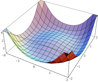
Figure 2.1:

Two-dimensional rotationally invariant potential: ${\cal V}(x,y)=-(x^{2}+y^{2})+\frac{(x^{2}+y^{2})^{2}}{4}$.

Now let us generalize the model to the case of an arbitrary compact Lie group $G$ of order $n_{G}$ resulting in $n_{G}$ infinitesimal generators. Once again, we start from a Lagrangian of the form [Goldstone:es]

$${\cal L}(\vec{\Phi},\partial_{\mu}\vec{\Phi})=\frac{1}{2}\partial_{\mu}\vec{\Phi}\cdot\partial^{\mu}\vec{\Phi}-{\cal V}(\vec{\Phi}),$$ (2.10)

where $\vec{\Phi}$ is a multiplet of scalar (or pseudoscalar) Hermitian fields. The Lagrangian ${\cal L}$ and thus also ${\cal V}(\vec{\Phi})$ are supposed to be globally invariant under $G$, where the infinitesimal transformations of the fields are given by

$$g\in G:\quad\Phi_{i}\to\Phi_{i}+\delta\Phi_{i},\quad\delta\Phi_{i}=-i\epsilon_{a}t^{a}_{ij}\Phi_{j}.$$ (2.11)

The Hermitian representation matrices $T^{a}=(t^{a}_{ij})$ are again antisymmetric and purely imaginary. We now assume that, by choosing an appropriate form of ${\cal V}$, the Lagrangian generates a spontaneous symmetry breaking resulting in a ground state with a vacuum expectation value $\vec{\Phi}_{\rm min}=\langle\vec{\Phi}\rangle$ which is invariant under a continuous subgroup $H$ of $G$. We expand ${\cal V}(\vec{\Phi})$ with respect to $\vec{\Phi}_{\rm min}$, $|\vec{\Phi}_{\rm min}|=v$, i.e., $\vec{\Phi}=\vec{\Phi}_{\rm min}+\vec{\chi}$,

$${\cal V}(\vec{\Phi})={\cal V}(\vec{\Phi}_{\rm min})+\underbrace{\frac{\partial{\cal V}(\vec{\Phi}_{\rm min})}{\partial\Phi_{i}}}_{\mbox{$0$}}\chi_{i}+\frac{1}{2}\underbrace{\frac{\partial^{2}{\cal V}(\vec{\Phi}_{\rm min})}{\partial\Phi_{i}\partial\Phi_{j}}}_{\mbox{$m^{2}_{ij}$}}\chi_{i}\chi_{j}+\cdots.$$ (2.12)

The matrix $M^{2}=(m^{2}_{ij})$ must be symmetric and, since one is expanding around a minimum, positive semidefinite, i.e.,

$$\sum_{i,j}m^{2}_{ij}x_{i}x_{j}\geq 0\quad\forall\quad\vec{x}.$$ (2.13)

In that case, all eigenvalues of $M^{2}$ are nonnegative. Making use of the invariance of ${\cal V}$ under the symmetry group $G$,

$${\cal V}(\vec{\Phi}_{\rm min}) = {\cal V}(D(g)\vec{\Phi}_{\rm min})={\cal V}(\vec{\Phi}_{\rm min}+\delta\vec{\Phi}_{\rm min})$$ (2.14)

$$\stackrel{{\scriptstyle\mbox{(\ref{3:2:venta})}}}{{=}} {\cal V}(\vec{\Phi}_{\rm min})+\frac{1}{2}m^{2}_{ij}\delta\Phi_{\rm min,i}\delta{\Phi}_{\rm min,j}+\cdots,$$

one obtains, by comparing coefficients,

$$m^{2}_{ij}\delta\Phi_{\rm min,i}\delta\Phi_{\rm min,j}=0.$$ (2.15)

Differentiating Eq. (2.15) with respect to $\delta\Phi_{\rm min,k}$ and using $m^{2}_{ij}=m^{2}_{ji}$ results in the matrix equation

$$M^{2}\delta\vec{\Phi}_{\rm min}=\vec{0}.$$ (2.16)

Inserting the variations of Eq. (2.11) for arbitrary $\epsilon_{a}$, $\delta\vec{\Phi}_{\rm min}=-i\epsilon_{a}T^{a}\vec{\Phi}_{\rm min}$, we conclude

$$M^{2}T^{a}\vec{\Phi}_{\rm min}=\vec{0}.$$ (2.17)

The solutions of Eq. (2.17) can be classified into two categories:

1. $T^{a}$, $a=1,\cdots,n_{H}$, is a representation of an element of the Lie algebra belonging to the subgroup $H$ of $G$, leaving the selected ground state invariant. In that case one has

   $$T^{a}\vec{\Phi}_{\rm min}=\vec{0},\quad a=1,\cdots,n_{H},$$

   such that Eq. (2.17) is automatically satisfied without any knowledge of $M^{2}$.

2. $T^{a}$, $a=n_{H}+1,\cdots,n_{G},$ is not a representation of an element of the Lie algebra belonging to the subgroup $H$. In that case $T^{a}\vec{\Phi}_{\rm min}\neq\vec{0}$, and $T^{a}\vec{\Phi}_{\rm min}$ is an eigenvector of $M^{2}$ with eigenvalue 0. To each such eigenvector corresponds a massless Goldstone boson. In particular, the different $T^{a}\vec{\Phi}_{\rm min}\neq\vec{0}$ are linearly independent, resulting in $n_{G}-n_{H}$ independent Goldstone bosons. (If they were not linearly independent, there would exist a nontrivial linear combination

   $$\vec{0}=\sum_{a=n_{H}+1}^{n_{G}}c_{a}(T^{a}\vec{\Phi}_{\rm min})=\underbrace{\left(\sum_{a=n_{H}+1}^{n_{G}}c_{a}T^{a}\right)}_{\mbox{$:=T$}}\vec{\Phi}_{\rm min},$$

   such that $T$ is an element of the Lie algebra of $H$ in contradiction to our assumption.)

Remark: It may be necessary to perform a similarity transformation on the fields in order to diagonalize the mass matrix.

Let us check these results by reconsidering the example of Eq. (2.1). In that case $n_{G}=3$ and $n_{H}=1$, generating 2 Goldstone bosons [see Eq. (2.1)].

We conclude this section with two remarks. First, the number of Goldstone bosons is determined by the structure of the symmetry groups. Let $G$ denote the symmetry group of the Lagrangian, with $n_{G}$ generators and $H$ the subgroup with $n_{H}$ generators which leaves the ground state after spontaneous symmetry breaking invariant. For each generator which does not annihilate the vacuum one obtains a massless Goldstone boson, i.e., the total number of Goldstone bosons equals $n_{G}-n_{H}$. Second, the Lagrangians used in motivating the phenomenon of a spontaneous symmetry breakdown are typically constructed in such a fashion that the degeneracy of the ground states is built into the potential at the classical level (the prototype being the “Mexican hat” potential of Fig. 2.1). As in the above case, it is then argued that an elementary Hermitian field of a multiplet transforming non-trivially under the symmetry group $G$ acquires a vacuum expectation value signaling a spontaneous symmetry breakdown. However, there also exist theories such as QCD where one cannot infer from inspection of the Lagrangian whether the theory exhibits spontaneous symmetry breaking. Rather, the criterion for spontaneous symmetry breaking is a non-vanishing vacuum expectation value of some Hermitian operator, not an elementary field, which is generated through the dynamics of the underlying theory. In particular, we will see that the quantities developing a vacuum expectation value may also be local Hermitian operators composed of more fundamental degrees of freedom of the theory. Such a possibility was already emphasized in the derivation of Goldstone’s theorem in Ref. [Goldstone:es].

2.2 Goldstone Theorem

By means of the above example, we motivate another approach to Goldstone’s theorem without delving into all the subtleties of a quantum field-theoretical approach (for further reading, see Chapter 2 of Ref. [Bernstein]). Given a Hamilton operator with a global symmetry group $G=\mbox{SO(3)}$, let $\vec{\Phi}(x)=(\Phi_{1}(x),\Phi_{2}(x),\Phi_{3}(x))$ denote a triplet of local Hermitian operators transforming as a vector under $G$,

$$g\in G: \vec{\Phi}(x)\mapsto\vec{\Phi}^{\prime}(x)=e^{i\sum_{k=1}^{3}\alpha_{k}Q_{k}}\vec{\Phi}(x)e^{-i\sum_{l=1}^{3}\alpha_{l}Q_{l}}$$ (2.18)

$$=e^{-i\sum_{k=1}^{3}\alpha_{k}T_{k}}\vec{\Phi}(x)\neq\vec{\Phi}(x),$$

where the $Q_{i}$ are the generators of the SO(3) transformations on the Hilbert space satisfying $[Q_{i},Q_{j}]=i\epsilon_{ijk}Q_{k}$ and the $T_{i}=(t^{i}_{jk})$ are the matrices of the three dimensional representation satisfying $t^{i}_{jk}=-i\epsilon_{ijk}$. We assume that one component of the multiplet acquires a non-vanishing vacuum expectation value:

$$\langle 0|\Phi_{1}(x)|0\rangle=\langle 0|\Phi_{2}(x)|0\rangle=0,\quad\langle 0|\Phi_{3}(x)|0\rangle=v\neq 0.$$ (2.19)

Then the two generators $Q_{1}$ and $Q_{2}$ do not annihilate the ground state, and to each such generator corresponds a massless Goldstone boson.

In order to prove these two statements let us expand Eq. (2.18) to first order in the $\alpha_{k}$:

$$\vec{\Phi}^{\prime}=\vec{\Phi}+i\sum_{k=1}^{3}\alpha_{k}[Q_{k},\vec{\Phi}]=\left(1-i\sum_{k=1}^{3}\alpha_{k}T_{k}\right)\vec{\Phi}=\vec{\Phi}+\vec{\alpha}\times\vec{\Phi}.$$

Comparing the terms linear in the $\alpha_{k}$

$$i[\alpha_{k}Q_{k},\Phi_{l}]=\epsilon_{lkm}\alpha_{k}\Phi_{m}$$

and noting that all three $\alpha_{k}$ can be chosen independently, we obtain

$$i[Q_{k},\Phi_{l}]=-\epsilon_{klm}\Phi_{m},$$

which, of course, simply expresses the fact that the field operators $\Phi_{i}$ transform as a vector. Using $\epsilon_{klm}\epsilon_{kln}=2\delta_{mn}$, we find

$$-\frac{i}{2}\epsilon_{kln}[Q_{k},\Phi_{l}]=\delta_{mn}\Phi_{m}=\Phi_{n}.$$

In particular,

$$\Phi_{3}=-\frac{i}{2}([Q_{1},\Phi_{2}]-[Q_{2},\Phi_{1}]),$$ (2.20)

with cyclic permutations for the other two cases.

In order to prove that $Q_{1}$ and $Q_{2}$ do not annihilate the ground state, let us consider Eq. (2.18) for $\vec{\alpha}=(0,\pi/2,0)$,

$$e^{-i\frac{\pi}{2}T_{2}}\vec{\Phi} = \left(\begin{array}[]{ccc}\cos(\pi/2)&0&\sin(\pi/2)\\ 0&1&0\\ -\sin(\pi/2)&0&\cos(\pi/2)\end{array}\right)\left(\begin{array}[]{c}\Phi_{1}\\ \Phi_{2}\\ \Phi_{3}\end{array}\right)=\left(\begin{array}[]{c}\Phi_{3}\\ \Phi_{2}\\ -\Phi_{1}\end{array}\right)$$

$$= e^{i\frac{\pi}{2}Q_{2}}\left(\begin{array}[]{c}\Phi_{1}\\ \Phi_{2}\\ \Phi_{3}\end{array}\right)e^{-i\frac{\pi}{2}Q_{2}}.$$

From the first row we obtain

$$\Phi_{3}=e^{i\frac{\pi}{2}Q_{2}}\Phi_{1}e^{-i\frac{\pi}{2}Q_{2}}.$$

Taking the vacuum expectation value

$$v=\langle 0|e^{i\frac{\pi}{2}Q_{2}}\Phi_{1}e^{-i\frac{\pi}{2}Q_{2}}|0\rangle$$

and using Eq. (2.19) clearly $Q_{2}|0\rangle\neq 0$, since otherwise the exponential operator could be replaced by unity and the right-hand side would vanish. A similar argument shows $Q_{1}|0\rangle\neq 0$.

At this point let us make two remarks.

• The “states” $Q_{1(2)}|0\rangle$ cannot be normalized. In a more rigorous derivation one makes use of integrals of the form

  $$\int d^{3}x\langle 0|[J^{0,b}(t,\vec{x}),\Phi_{c}(0)]|0\rangle,$$

  and first determines the commutator before evaluating the integral [Bernstein].

• Some derivations of Goldstone’s theorem right away start by assuming $Q_{1(2)}|0\rangle$ $\neq 0$. However, for the discussion of spontaneous symmetry breaking in the framework of QCD it is advantageous to establish the connection between the existence of Goldstone bosons and a non-vanishing expectation value (see Section 3.2).

Let us now turn to the existence of Goldstone bosons, taking the vacuum expectation value of Eq. (2.20):

$$0\neq v=\langle 0|\Phi_{3}(0)|0\rangle=-\frac{i}{2}\langle 0|\left([Q_{1},\Phi_{2}(0)]-[Q_{2},\Phi_{1}(0)]\right)|0\rangle\equiv-\frac{i}{2}(A-B).$$

We will first show $A=-B$. To that end we perform a rotation of the fields as well as the generators by $\pi/2$ about the 3 axis [see Eq. (2.18) with $\vec{\alpha}=(0,0,\pi/2)$]:

$$e^{-i\frac{\pi}{2}T_{3}}\vec{\Phi} = \left(\begin{array}[]{r}-\Phi_{2}\\ \Phi_{1}\\ \Phi_{3}\end{array}\right)=e^{i\frac{\pi}{2}Q_{3}}\left(\begin{array}[]{c}\Phi_{1}\\ \Phi_{2}\\ \Phi_{3}\end{array}\right)e^{-i\frac{\pi}{2}Q_{3}},$$

and analogously for the charge operators

$$\left(\begin{array}[]{r}-Q_{2}\\ Q_{1}\\ Q_{3}\end{array}\right)=e^{i\frac{\pi}{2}Q_{3}}\left(\begin{array}[]{r}Q_{1}\\ Q_{2}\\ Q_{3}\end{array}\right)e^{-i\frac{\pi}{2}Q_{3}}.$$

We thus obtain

$$B=\langle 0|[Q_{2},\Phi_{1}(0)]|0\rangle = \langle 0|\Big{(}e^{i\frac{\pi}{2}Q_{3}}(-Q_{1})\underbrace{e^{-i\frac{\pi}{2}Q_{3}}e^{i\frac{\pi}{2}Q_{3}}}_{\mbox{1}}\Phi_{2}(0)e^{-i\frac{\pi}{2}Q_{3}}$$

$$-e^{i\frac{\pi}{2}Q_{3}}\Phi_{2}(0)e^{-i\frac{\pi}{2}Q_{3}}e^{i\frac{\pi}{2}Q_{3}}(-Q_{1})e^{-i\frac{\pi}{2}Q_{3}}\Big{)}|0\rangle$$

$$= -\langle 0|[Q_{1},\Phi_{2}(0)]|0\rangle=-A,$$

where we made use of $Q_{3}|0\rangle=0$, i.e., the vacuum is invariant under rotations about the 3 axis. In other words, the non-vanishing vacuum expectation value $v$ can also be written as

$$0\neq v = \langle 0|\Phi_{3}(0)|0\rangle=-i\langle 0|[Q_{1},\Phi_{2}(0)]|0\rangle$$ (2.24)

$$= -i\int d^{3}x\langle 0|[J^{1}_{0}(t,\vec{x}),\Phi_{2}(0)]|0\rangle.$$

We insert a complete set of states $1=\sum_{n}\int\hskip 5.0pt|n\rangle\langle n|$ into the commutator

$$v = -i\sum_{n}\int\int d^{3}x\left(\langle 0|J^{1}_{0}(t,\vec{x})|n\rangle\langle n|\Phi_{2}(0)|0\rangle-\langle 0|\Phi_{2}(0)|n\rangle\langle n|J^{1}_{0}(t,\vec{x})|0\rangle\right),$$

and make use of translational invariance

$$= -i\sum_{n}\int\int d^{3}x\left(e^{-iP_{n}\cdot x}\langle 0|J^{1}_{0}(0)|n\rangle\langle n|\Phi_{2}(0)|0\rangle-\cdots\right)$$

$$= -i\sum_{n}\int(2\pi)^{3}\delta^{3}(\vec{P}_{n})\left(e^{-iE_{n}t}\langle 0|J^{1}_{0}(0)|n\rangle\langle n|\Phi_{2}(0)|0\rangle\right.$$

$$\left.-e^{iE_{n}t}\langle 0|\Phi_{2}(0)|n\rangle\langle n|J^{1}_{0}(0)|0\rangle\right).$$

Integration with respect to the momentum of the inserted intermediate states yields an expression of the form

$$=-i(2\pi)^{3}\sum_{n}^{\prime}\left(e^{-iE_{n}t}\cdots-e^{iE_{n}t}\cdots\right),$$

where the prime indicates that only states with $\vec{P}=0$ need to be considered. Due to the Hermiticity of the symmetry current operators $J^{\mu,a}$ as well as the $\Phi_{l}$, we have

$$c_{n}:=\langle 0|J^{1}_{0}(0)|n\rangle\langle n|\Phi_{2}(0)|0\rangle=\langle n|J^{1}_{0}(0)|0\rangle^{\ast}\langle 0|\Phi_{2}(0)|n\rangle^{\ast},$$

such that

$$v=-i(2\pi)^{3}\sum_{n}^{\prime}\left(c_{n}e^{-iE_{n}t}-c_{n}^{\ast}e^{iE_{n}t}\right).$$ (2.25)

From Eq. (2.25) we draw the following conclusions.

1. Due to our assumption of a non-vanishing vacuum expectation value $v$, there must exist states $|n\rangle$ for which both $\langle 0|J^{0}_{1(2)}(0)|n\rangle$ and$\langle n|\Phi_{1(2)}(0)|0\rangle$ do not vanish. The vacuum itself cannot contribute to Eq. (2.25) because $\langle 0|\Phi_{1(2)}(0)|0\rangle=0$.

2. States with $E_{n}>0$ contribute ($\varphi_{n}$ is the phase of $c_{n}$)

   $$\frac{1}{i}\left(c_{n}e^{-iE_{n}t}-c_{n}^{\ast}e^{iE_{n}t}\right) = \frac{1}{i}|c_{n}|\left(e^{i\varphi_{n}}e^{-iE_{n}t}-e^{-i\varphi_{n}}e^{iE_{n}t}\right)$$

   $$= 2|c_{n}|\sin(\varphi_{n}-E_{n}t)$$

   to the sum. However, $v$ is time-independent and therefore the sum over states with $(E_{n}>0,\vec{0})$ must vanish.

3. The right-hand side of Eq. (2.25) must therefore contain the contribution from states with zero energy as well as zero momentum thus zero mass. These zero-mass states are the Goldstone bosons.

2.3 Explicit Symmetry Breaking: A First Look *

Finally, let us illustrate the consequences of adding to our Lagrangian of Eq. (2.1) a small perturbation which explicitly breaks the symmetry. To that end, we modify the potential of Eq. (2.1) by adding a term $a\Phi_{3}$,

$${\cal V}(\Phi_{1},\Phi_{2},\Phi_{3})=\frac{m^{2}}{2}\Phi_{i}\Phi_{i}+\frac{\lambda}{4}(\Phi_{i}\Phi_{i})^{2}+a\Phi_{3},$$ (2.26)

where $m^{2}<0$, $\lambda>0$, and $a>0$, with Hermitian fields $\Phi_{i}$. Clearly, the potential no longer has the original O(3) symmetry but is only invariant under O(2). The conditions for the new minimum, obtained from $\vec{\nabla}_{\Phi}{\cal V}=0$, read

$$\Phi_{1}=\Phi_{2}=0,\quad\lambda\Phi_{3}^{3}+m^{2}\Phi_{3}+a=0.$$

Exercise 2.3.1

Solve the cubic equation for $\Phi_{3}$ using the perturbative ansatz

$$\langle\Phi_{3}\rangle=\Phi^{(0)}_{3}+a\Phi^{(1)}_{3}+{\cal O}(a^{2}).$$ (2.27)

The solution reads

$$\Phi^{(0)}_{3}=\pm\sqrt{-\frac{m^{2}}{\lambda}},\quad\Phi^{(1)}_{3}=\frac{1}{2m^{2}}.$$

Of course, $\Phi^{(0)}_{3}$ corresponds to our result without explicit perturbation. The condition for a minimum [see Eq. (2.13)] excludes $\Phi^{(0)}_{3}=+\sqrt{-\frac{m^{2}}{\lambda}}$. Expanding the potential with $\Phi_{3}=\langle\Phi_{3}\rangle+\eta$ we obtain, after a short calculation, for the masses

$$m_{\Phi_{1}}^{2}=m_{\Phi_{2}}^{2} = a\sqrt{\frac{\lambda}{-m^{2}}},$$

$$m_{\eta}^{2} = -2m^{2}+3a\sqrt{\frac{\lambda}{-m^{2}}}.$$ (2.28)

The important feature here is that the original Goldstone bosons of Eq. (2.1) are now massive. The squared masses are proportional to the symmetry breaking parameter $a$. Calculating quantum corrections to observables in terms of Goldstone-boson loop diagrams will generate corrections which are non-analytic in the symmetry breaking parameter such as $a\ln(a)$. Such so-called chiral logarithms originate from the mass terms in the Goldstone boson propagators entering the calculation of loop integrals. We will come back to this point in the next Chapter when we discuss the masses of the pseudoscalar octet in terms of the quark masses which, in QCD, represent the analogue to the parameter $a$ in the above example.

Chapter 3 Chiral Perturbation Theory for Mesons

Chiral perturbation theory provides a systematic method for discussing the consequences of the global flavor symmetries of QCD at low energies by means of an effective field theory. The effective Lagrangian is expressed in terms of those hadronic degrees of freedom which, at low energies, show up as observable asymptotic states. At very low energies these are just the members of the pseudoscalar octet ($\pi,K,\eta$) which are regarded as the Goldstone bosons of the spontaneous breaking of the chiral $\mbox{SU(3)}_{L}\times\mbox{SU}(3)_{R}$ symmetry down to $\mbox{SU}(3)_{V}$. The non-vanishing masses of the light pseudoscalars in the “real” world are related to the explicit symmetry breaking in QCD due to the light quark masses.

3.1 Effective Field Theory

Chiral perturbation theory is an example of an effective field theory (EFT). Before discussing chiral perturbation theory in detail we want to briefly outline some of the main features of the effective field theory approach, as it finds a wide range of applications in physics.

The basic idea of an EFT is that one does not need to know everything in order to make a sensible description of the particular part of physics one is interested in. In general, effective field theories are low-energy approximations to more fundamental theories. Instead of solving the underlying theory, low-energy physics is described with a set of variables that is suited for the particular energy region you are interested in. The effective field theory can then be used to calculate physical quantities in terms of an expansion in $p/\Lambda$, where $p$ stands for momenta or masses that are smaller than a certain momentum scale $\Lambda$. By suited we mean that the description in the low-energy degrees of freedom is more convenient for actual calculations. For example, we will use pions and nucleons instead of the more fundamental quarks and gluons as the degrees of freedom in low-energy processes in hadronic physics. This is more convenient since so far we do not know how to solve QCD, and standard perturbation theory cannot be applied for energies well below $1\ \rm{GeV}$. It should be noted that an effective field theory only has a limited range of applicability, since it gives the wrong high-energy behavior. After all, it is not the same as the underlying theory. But as long as one stays well below the momentum scale $\Lambda$, the EFT is designed to give an appropriate description up to finite accuracy, as in actual calculations only a finite number of terms in the expansion in $p/\Lambda$ has to be considered.

In order to construct an EFT one has to write down the effective Lagrangian, which includes all terms that are compatible with the symmetries of the underlying theory. This means that the Lagrangian actually consists of an infinite number of terms. The coefficients of these terms should in principle be calculable from the underlying theory. In the case of chiral perturbation theory, however, we cannot yet solve the underlying theory, QCD, and the parameters are taken as free parameters that are fitted to experimental data. The second important ingredient together with the effective Lagrangian is a method that allows to decide which terms contribute in a calculation up to a certain accuracy. We will see an example of such a method when considering Weinberg’s power counting in Section 3.5.

Effective field theories are non-renormalizable in the traditional sense. However, as long as one considers all terms that are allowed by the symmetries, divergences that occur in calculations up to any given order of $p/\Lambda$ can be renormalized by redefining fields and parameters of the Lagrangian of the effective field theory.

3.2 Spontaneous Symmetry Breaking in QCD

While the toy model of Section 2.1 by construction led to a spontaneous symmetry breaking, it is not fully understood theoretically why QCD should exhibit this phenomenon. We will first motivate why experimental input, the hadron spectrum of the “real” world, indicates that spontaneous symmetry breaking happens in QCD. Secondly, we will show that a non-vanishing singlet scalar quark condensate is a sufficient condition for a spontaneous symmetry breaking in QCD.

3.2.1 The Hadron Spectrum

We saw in Section 1.3 that the QCD Lagrangian possesses an $\mbox{SU(3)}_{L}\times\mbox{SU(3)}_{R}\times\mbox{U(1)}_{V}$ symmetry in the chiral limit in which the light quark masses vanish. From symmetry considerations involving the Hamiltonian $H^{0}_{\rm QCD}$ only, one would naively expect that hadrons organize themselves into approximately degenerate multiplets fitting the dimensionalities of irreducible representations of the group $\mbox{SU(3)}_{L}\times\mbox{SU(3)}_{R}\times\mbox{U(1)}_{V}$. The $\mbox{U(1)}_{V}$ symmetry results in baryon number conservation and leads to a classification of hadrons into mesons ($B=0$) and baryons ($B=1$). The linear combinations $Q^{a}_{V}=Q^{a}_{R}+Q^{a}_{L}$ and $Q^{a}_{A}=Q^{a}_{R}-Q^{a}_{L}$ of the left- and right-handed charge operators commute with $H^{0}_{\rm QCD}$, have opposite parity, and thus for any state of positive parity one would expect the existence of a degenerate state of negative parity (parity doubling) which can be seen as follows. Let $|i,+\rangle$ denote an eigenstate of $H^{0}_{\rm QCD}$ with eigenvalue $E_{i}$,

$$H^{0}_{\rm QCD}|i,+\rangle=E_{i}|i,+\rangle,$$

having positive parity,

$$P|i,+\rangle=+|i,+\rangle,$$

such as, e.g., a member of the ground state baryon octet (in the chiral limit). Defining $|\phi\rangle=Q_{A}^{a}|i,+\rangle$, because of $[H^{0}_{\rm QCD},Q_{A}^{a}]=0$, we have

$$H^{0}_{\rm QCD}|\phi\rangle=H^{0}_{\rm QCD}Q_{A}^{a}|i,+\rangle=Q_{A}^{a}H^{0}_{\rm QCD}|i,+\rangle=E_{i}Q_{A}^{a}|i,+\rangle=E_{i}|\phi\rangle,$$

i.e, the new state $|\phi\rangle$ is also an eigenstate of $H^{0}_{\rm QCD}$ with the same eigenvalue $E_{i}$ but of opposite parity:

$$P|\phi\rangle=PQ_{A}^{a}P^{-1}P|i,+\rangle=-Q_{A}^{a}(+|i,+\rangle)=-|\phi\rangle.$$

The state $|\phi\rangle$ can be expanded in terms of the members of the multiplet with negative parity,

$$|\phi\rangle=Q^{a}_{A}|i,+\rangle=-t^{a}_{ij}|j,-\rangle.$$

However, the low-energy spectrum of baryons does not contain a degenerate baryon octet of negative parity. Naturally the question arises whether the above chain of arguments is incomplete. Indeed, we have tacitly assumed that the ground state of QCD is annihilated by $Q^{a}_{A}$.

Let $a^{\dagger}_{i}$ symbolically denote an operator which creates quanta with the quantum numbers of the state $|i,+\rangle$, whereas $b_{i}^{\dagger}$ creates degenerate quanta of opposite parity. Let us assume the states $|i,+\rangle$ and $|i,-\rangle$ to be linear combinations which are constructed from members of two bases carrying irreducible representations of $\mbox{SU(3)}_{L}\times\mbox{SU(3)}_{R}$. In analogy to Eq. (1.90), we assume that under $\mbox{SU(3)}_{L}\times\mbox{SU(3)}_{R}$ the creation operators are related by

$$[Q^{a}_{A},a^{\dagger}_{i}]=-t^{a}_{ij}b_{j}^{\dagger}.$$

The usual chain of arguments then works as

$$Q^{a}_{A}|i,+\rangle = Q^{a}_{A}a^{\dagger}_{i}|0\rangle=\Big{(}[Q^{a}_{A},a^{\dagger}_{i}]+a_{i}^{\dagger}\underbrace{Q_{A}^{a}}_{\mbox{$\hookrightarrow 0$}}\Big{)}|0\rangle=-t^{a}_{ij}b_{j}^{\dagger}|0\rangle.$$ (3.1)

However, if the ground state is not annihilated by $Q_{A}^{a}$, the reasoning of Eq. (3.1) does no longer apply. In that case the ground state is not invariant under the full symmetry group of the Lagrangian resulting in a spontaneous symmetry breaking. In other words, the non-existence of degenerate multiplets of opposite parity points to the fact that SU(3) instead of $\mbox{SU(3)}_{L}\times\mbox{SU(3)}_{R}$ is approximately realized as a symmetry of the hadrons. Furthermore the octet of the pseudoscalar mesons is special in the sense that the masses of its members are small in comparison with the corresponding $1^{-}$ vector mesons. They are candidates for the Goldstone bosons of a spontaneous symmetry breaking.

In order to understand the origin of the SU(3) symmetry let us consider the vector charges $Q^{a}_{V}=Q_{R}^{a}+Q^{a}_{L}$ [see Eq. (1.126)]. They satisfy the commutation relations of an SU(3) Lie algebra [see Eqs. (1.138) - (1.140)],

$$[Q_{R}^{a}+Q_{L}^{a},Q_{R}^{b}+Q_{L}^{b}]=[Q_{R}^{a},Q_{R}^{b}]+[Q_{L}^{a},Q_{L}^{b}]=if_{abc}Q_{R}^{c}+if_{abc}Q_{L}^{c}=if_{abc}Q^{c}_{V}.$$ (3.2)

It was shown by Vafa and Witten [Vafa:tf:1:1] that, in the chiral limit, the ground state is necessarily invariant under $\mbox{SU(3)}_{V}\times\mbox{U(1)}_{V}$, i.e., the eight vector charges $Q^{a}_{V}$ as well as the baryon number operator $Q_{V}/3$ annihilate the ground state,

$$Q^{a}_{V}|0\rangle=Q_{V}|0\rangle=0.$$ (3.3)

If the vacuum is invariant under $\mbox{SU(3)}_{V}\times\mbox{U(1)}_{V}$, then so is the Hamiltonian (but not vice versa) (Coleman’s theorem [Coleman:1966:1:1]). Moreover, the invariance of the ground state and the Hamiltonian implies that the physical states of the spectrum of $H^{0}_{\rm QCD}$ can be organized according to irreducible representations of $\mbox{SU(3)}_{V}\times\mbox{U(1)}_{V}$. The index $V$ (for vector) indicates that the generators result from integrals of the zeroth component of vector current operators and thus transform with a positive sign under parity.

Let us now turn to the linear combinations $Q^{a}_{A}=Q^{a}_{R}-Q^{a}_{L}$ satisfying the commutation relations [see Eqs. (1.138) - (1.140)]

$$[Q^{a}_{A},Q^{b}_{A}] = [Q^{a}_{R}-Q^{a}_{L},Q^{b}_{R}-Q^{b}_{L}]=[Q^{a}_{R},Q^{b}_{R}]+[Q^{a}_{L},Q^{b}_{L}]$$

$$= if_{abc}Q^{c}_{R}+if_{abc}Q^{c}_{L}=if_{abc}Q^{c}_{V},$$

$${[Q_{V}^{a},Q^{b}_{A}]} = [Q_{R}^{a}+Q_{L}^{a},Q_{R}^{b}-Q_{L}^{b}]=[Q_{R}^{a},Q^{b}_{R}]-[Q^{a}_{L},Q^{b}_{L}]$$ (3.4)

$$= if_{abc}Q^{c}_{R}-if_{abc}Q^{c}_{L}=if_{abc}Q^{c}_{A}.$$

Note that these charge operators do not form a closed algebra, i.e., the commutator of two axial charge operators is not again an axial charge operator. Since the parity doubling is not observed for the low-lying states, one assumes that the $Q_{A}^{a}$ do not annihilate the ground state,

$$Q^{a}_{A}|0\rangle\neq 0,$$ (3.5)

i.e., the ground state of QCD is not invariant under “axial” transformations. According to Goldstone’s theorem, to each axial generator $Q^{a}_{A}$, which does not annihilate the ground state, corresponds a massless Goldstone boson field $\phi^{a}(x)$ with spin 0, whose symmetry properties are tightly connected to the generator in question. The Goldstone bosons have the same transformation behavior under parity,

$$\phi^{a}(t,\vec{x})\stackrel{{\scriptstyle P}}{{\mapsto}}-\phi^{a}(t,-\vec{x}),$$ (3.6)

i.e., they are pseudoscalars, and transform under the subgroup $H=\mbox{SU(3)}_{V}$, which leaves the vacuum invariant, as an octet [see Eq. (3.4)]:

$$[Q^{a}_{V},\phi^{b}(x)]=if_{abc}\phi^{c}(x).$$ (3.7)

In the present case, $G=\mbox{SU(3)}_{L}\times\mbox{SU(3)}_{R}$ with $n_{G}=16$ and $H=\mbox{SU(3)}_{V}$ with $n_{H}=8$ and we expect eight Goldstone bosons.

3.2.2 The Scalar Quark Condensate *

In the following, we will show that a non-vanishing scalar quark condensate in the chiral limit is a sufficient (but not a necessary) condition for a spontaneous symmetry breaking in QCD. The subsequent discussion will parallel that of the toy model in Section 2.2 after replacement of the elementary fields $\Phi_{i}$ by appropriate composite Hermitian operators of QCD.

Let us first recall the definition of the nine scalar and pseudoscalar quark densities:

$$S_{a}(y) = \bar{q}(y)\lambda_{a}q(y),\quad a=0,\cdots,8,$$ (3.8)

$$P_{a}(y) = i\bar{q}(y)\gamma_{5}\lambda_{a}q(y),\quad a=0,\cdots,8.$$ (3.9)

Exercise 3.2.1

Show that $S_{a}$ and $P_{a}$ transform under $\mbox{SU(3)}_{L}\times\mbox{SU(3)}_{R}$, i.e., $q_{L}\mapsto q_{L}^{\prime}=U_{L}q_{L}$ and $q_{R}\mapsto q_{R}^{\prime}=U_{R}q_{R}$, as

$$S_{a} \mapsto S_{a}^{\prime}=\bar{q}_{L}U_{L}^{\dagger}\lambda_{a}U_{R}q_{R}+\bar{q}_{R}U_{R}^{\dagger}\lambda_{a}U_{L}q_{L},$$

$$P_{a} \mapsto P_{a}^{\prime}=i\bar{q_{L}}U_{L}^{\dagger}\lambda_{a}U_{R}q_{R}-i\bar{q}_{R}U_{R}^{\dagger}\lambda_{a}U_{L}q_{L}.$$

Hint: Express $S_{a}$ and $P_{a}$ in terms of left- and right-handed quark fields. What are $\gamma_{5}P_{R}$ and $\gamma_{5}P_{L}$?

In technical terms: The components $S_{a}$ transform as members of a $(3^{\ast},3)+(3,3^{\ast})$ representation.

The equal-time commutation relation of two quark operators of the form $A_{i}(x)=q^{\dagger}(x)\hat{A}_{i}q(x)$, where $\hat{A}_{i}$ symbolically denotes Dirac- and flavor matrices and a summation over color indices is implied, can compactly be written as [see Eq. (1.3.5)]

$$[A_{1}(t,\vec{x}),A_{2}(t,\vec{y})]=\delta^{3}(\vec{x}-\vec{y})q^{\dagger}(x)[\hat{A}_{1},\hat{A}_{2}]q(x).$$ (3.10)

With the definition

$$Q_{V}^{a}(t)=\int d^{3}xq^{\dagger}(t,\vec{x})\frac{\lambda^{a}}{2}q(t,\vec{x}),$$

and using

$$[\frac{\lambda_{a}}{2},\gamma_{0}\lambda_{0}] = 0,$$

$${[}\frac{\lambda_{a}}{2},\gamma_{0}\lambda_{b}] = \gamma_{0}if_{abc}\lambda_{c},$$

we see, after integration of Eq. (3.10) over $\vec{x}$, that the scalar quark densities of Eq. (3.8) transform under $\mbox{SU(3)}_{V}$ as a singlet and as an octet, respectively,

$$[Q^{a}_{V}(t),S_{0}(y)] = 0,\quad a=1,\cdots,8,$$ (3.11)

$${[Q^{a}_{V}(t),S_{b}(y)]} = i\sum_{c=1}^{8}f_{abc}S_{c}(y),\quad a,b=1,\cdots,8,$$ (3.12)

with analogous results for the pseudoscalar quark densities. In the $\mbox{SU(3)}_{V}$ limit and, of course, also in the even more restrictive chiral limit, the charge operators in Eqs. (3.11) and (3.12) are actually time independent. Using the relation

$$\sum_{a,b=1}^{8}f_{abc}f_{abd}=3\delta_{cd}$$ (3.13)

for the structure constants of SU(3), we re-express the octet components of the scalar quark densities as

$$S_{a}(y)=-\frac{i}{3}\sum_{b,c=1}^{8}f_{abc}[Q_{V}^{b}(t),S_{c}(y)],$$ (3.14)

which represents the analogue of Eq. (2.20) in the discussion of Goldstone’s theorem.

In the chiral limit the ground state is necessarily invariant under $\mbox{SU(3)}_{V}$, i.e., $Q_{V}^{a}|0\rangle=0$, and we obtain from Eq. (3.14)

$$\langle 0|S_{a}(y)|0\rangle=\langle 0|S_{a}(0)|0\rangle\equiv\langle S_{a}\rangle=0,\quad a=1,\cdots,8,$$ (3.15)

where we made use of translational invariance of the ground state. In other words, the octet components of the scalar quark condensate must vanish in the chiral limit. From Eq. (3.15), we obtain for $a=3$

$$\langle\bar{u}u\rangle-\langle\bar{d}d\rangle=0,$$

i.e. $\langle\bar{u}u\rangle=\langle\bar{d}d\rangle$ and for $a=8$

$$\langle\bar{u}u\rangle+\langle\bar{d}d\rangle-2\langle\bar{s}s\rangle=0,$$

i.e. $\langle\bar{u}u\rangle=\langle\bar{d}d\rangle=\langle\bar{s}s\rangle$.

Because of Eq. (3.11) a similar argument cannot be used for the singlet condensate, and if we assume a non-vanishing singlet scalar quark condensate in the chiral limit, we find using $\langle\bar{u}u\rangle=\langle\bar{d}d\rangle=\langle\bar{s}s\rangle$:

$$0\neq\langle\bar{q}q\rangle=\langle\bar{u}u+\bar{d}d+\bar{s}s\rangle=3\langle\bar{u}u\rangle=3\langle\bar{d}d\rangle=3\langle\bar{s}s\rangle.$$ (3.16)

Finally, we make use of (no summation implied!)

$$(i)^{2}[\gamma_{5}\frac{\lambda_{a}}{2},\gamma_{0}\gamma_{5}\lambda_{a}]=\lambda^{2}_{a}\gamma_{0}$$

in combination with

$$\lambda_{1}^{2}=\lambda_{2}^{2}=\lambda_{3}^{2} = \left(\begin{array}[]{rrr}1&0&0\\ 0&1&0\\ 0&0&0\end{array}\right),$$

$$\lambda_{4}^{2}=\lambda_{5}^{2} = \left(\begin{array}[]{rrr}1&0&0\\ 0&0&0\\ 0&0&1\end{array}\right),$$

$$\lambda_{6}^{2}=\lambda_{7}^{2} = \left(\begin{array}[]{rrr}0&0&0\\ 0&1&0\\ 0&0&1\end{array}\right),$$

$$\lambda_{8}^{2} = \frac{1}{3}\left(\begin{array}[]{rrr}1&0&0\\ 0&1&0\\ 0&0&4\end{array}\right)$$

to obtain

$$i[Q_{a}^{A}(t),P_{a}(y)]=\left\{\begin{array}[]{cl}\bar{u}u+\bar{d}d,&a=1,2,3\\ \bar{u}u+\bar{s}s,&a=4,5\\ \bar{d}d+\bar{s}s,&a=6,7\\ \frac{1}{3}(\bar{u}u+\bar{d}d+4\bar{s}s),&a=8\end{array}\right.$$ (3.21)

where we have suppressed the $y$ dependence on the right-hand side. We evaluate Eq. (3.21) for a ground state which is invariant under $\mbox{SU(3)}_{V}$, assuming a non-vanishing singlet scalar quark condensate,

$$\langle 0|i[Q_{a}^{A}(t),P_{a}(y)]|0\rangle=\frac{2}{3}\langle\bar{q}q\rangle,\quad a=1,\cdots,8,$$ (3.22)

where, because of translational invariance, the right-hand side is independent of $y$. Inserting a complete set of states into the commutator of Eq. (3.22) yields, in complete analogy to Section 2.2 [see the discussion following Eq. (2.24)] that both the pseudoscalar density $P_{a}(y)$ as well as the axial charge operators $Q^{a}_{A}$ must have a non-vanishing matrix element between the vacuum and massless one particle states $|\phi^{b}\rangle$. In particular, because of Lorentz covariance, the matrix element of the axial-vector current operator between the vacuum and these massless states, appropriately normalized, can be written as

$$\langle 0|A^{a}_{\mu}(0)|\phi^{b}(p)\rangle=ip_{\mu}F_{0}\delta^{ab},$$ (3.23)

where $F_{0}\approx 93$ MeV denotes the “decay” constant of the Goldstone bosons in the chiral limit. From Eq. (3.23) we see that a non-zero value of $F_{0}$ is a necessary and sufficient criterion for spontaneous chiral symmetry breaking. On the other hand, because of Eq. (3.22) a non-vanishing scalar quark condensate $\langle\bar{q}q\rangle$ is a sufficient (but not a necessary) condition for a spontaneous symmetry breakdown in QCD.

Table 3.1 contains a summary of the patterns of spontaneous symmetry breaking as discussed in Section 2.2, the generalization of Section 2.1 to the so-called O($N$) linear sigma model, and QCD.

	Section 2.2	O($N$) linear	QCD
		sigma model
Symmetry group $G$ of	O(3)	O($N$)	$\mbox{SU(3)}_{L}\times\mbox{SU(3)}_{R}$
the Lagrangian density
Number of	3	$N(N-1)/2$	16
generators $n_{G}$
Symmetry group $H$	O(2)	O($N-1$)	SU(3)V
of the ground state
Number of	1	$(N-1)(N-2)/2$	8
generators $n_{H}$
Number of
Goldstone bosons	2	$N-1$	8
$n_{G}-n_{H}$
Multiplet of	$(\Phi_{1}(x),\Phi_{2}(x))$	$(\Phi_{1}(x),\cdots,\Phi_{N-1}(x))$	$i\bar{q}(x)\gamma_{5}\lambda_{a}q(x)$
Goldstone boson fields
Vacuum expectation	$v=\langle\Phi_{3}\rangle$	$v=\langle\Phi_{N}\rangle$	$v=\langle\bar{q}q\rangle$
value

Table 3.1: Comparison of spontaneous symmetry breaking.

3.3 Transformation Properties of the Goldstone Bosons

The purpose of this section is to discuss the transformation properties of the field variables describing the Goldstone bosons. We will need the concept of a nonlinear realization of a group in addition to a representation of a group which one usually encounters in Physics. We will first discuss a few general group-theoretical properties before specializing to QCD.

3.3.1 General Considerations *

Let us consider a physical system with a Hamilton operator $\hat{H}$ which is invariant under a compact Lie group $G$. Furthermore we assume the ground state of the system to be invariant under only a subgroup $H$ of $G$, giving rise to $n=n_{G}-n_{H}$ Goldstone bosons. Each of these Goldstone bosons will be described by an independent field $\phi_{i}$ which is a continuous real function on Minkowski space $M^{4}$. We collect these fields in an $n$-component vector $\Phi$ and define the vector space

$$M_{1}\equiv\{\Phi:M^{4}\to R^{n}|\phi_{i}:M^{4}\to R\,\,\mbox{continuous}\}.$$ (3.24)

Our aim is to find a mapping $\varphi$ which uniquely associates with each pair $(g,\Phi)\in G\times M_{1}$ an element $\varphi(g,\Phi)\in M_{1}$ with the following properties:

$$\varphi(e,\Phi)=\Phi\,\,\forall\,\,\Phi\in M_{1},\,e\,\,\mbox{identity of}\,\,G,$$ (3.25)

$$\varphi(g_{1},\varphi(g_{2},\Phi))=\varphi(g_{1}g_{2},\Phi)\,\,\forall\,\,g_{1},g_{2}\in G,\,\forall\,\Phi\in M_{1}.$$ (3.26)

Such a mapping defines an operation of the group $G$ on $M_{1}$. The second condition is the so-called group-homomorphism property. The mapping will, in general, not define a representation of the group $G$, because we do not require the mapping to be linear, i.e., $\varphi(g,\lambda\Phi)\neq\lambda\varphi(g,\Phi)$.

Let $\Phi=0$ denote the “origin” of $M_{1}$ which, in a theory containing Goldstone bosons only, loosely speaking corresponds to the ground state configuration. Since the ground state is supposed to be invariant under the subgroup $H$ we require the mapping $\varphi$ to be such that all elements $h\in H$ map the origin onto itself. In this context the subgroup $H$ is also known as the little group of $\Phi=0$. Given that such a mapping indeed exists, we need to verify for infinite groups that:

1. $H$ is not empty, because the identity $e$ maps the origin onto itself.

2. If $h_{1}$ and $h_{2}$ are elements satisfying $\varphi(h_{1},0)=\varphi(h_{2},0)=0$, so does $\varphi(h_{1}h_{2},0)=\varphi(h_{1},\varphi(h_{2},0))=\varphi(h_{1},0)=0$, i.e., because of the homomorphism property also the product $h_{1}h_{2}\in H$.

3. For $h\in H$ we have

   $$\varphi(h^{-1},0)=\varphi(h^{-1},\varphi(h,0))=\varphi(h^{-1}h,0)=\varphi(e,0),$$

   i.e., $h^{-1}\in H$.

We will establish a connection between the Goldstone boson fields and the set of all left cosets $\{gH|g\in G\}$ which is also referred to as the quotient $G/H$. For a subgroup $H$ of $G$ the set $gH=\{gh|h\in H\}$ defines the left coset of $g$ (with an analogous definition for the right coset) which is one element of $G/H$. For our purposes we need the property that cosets either completely overlap or are completely disjoint, i.e, the quotient is a set whose elements themselves are sets of group elements, and these sets are completely disjoint.

• As an illustration, consider the symmetry group $C_{4}$ of a square with directed sides:

$$G=C_{4} = \{e,a,a^{2},a^{3}\},\quad\mbox{$a$ rotation by 90${}^{\circ}$},\quad a^{4}=e,$$

$$H = \{e,a^{2}\}.$$

$$eH=\{e,a^{2}\},\,\,aH=\{a,a^{3}\},\,\,a^{2}H=\{e,a^{2}\},\,\,a^{3}H=\{a,a^{3}\}.$$

$$G/H=\{gH|g\in G\}=\{\{e,a^{2}\},\{a,a^{3}\}\}.$$

Let us first show that for all elements of a given coset, $\varphi$ maps the origin onto the same vector in $R^{n}$:

$$\varphi(gh,0)=\varphi(g,\varphi(h,0))=\varphi(g,0)\,\,\forall\,\,g\in G\,\mbox{and}\,h\in H.$$

Secondly, the mapping is injective with respect to the elements of $G/H$, which can be proven as follows. Consider two elements $g$ and $g^{\prime}$ of $G$ where $g^{\prime}\not\in gH$. We need to show $\varphi(g,0)\neq\varphi(g^{\prime},0)$. Let us assume $\varphi(g,0)=\varphi(g^{\prime},0)$:

$$0=\varphi(e,0)=\varphi(g^{-1}g,0)=\varphi(g^{-1},\varphi(g,0))=\varphi(g^{-1},\varphi(g^{\prime},0))=\varphi(g^{-1}g^{\prime},0).$$

However, this implies $g^{-1}g^{\prime}\in H$ or $g^{\prime}\in gH$ in contradiction to the assumption. Thus $\varphi(g,0)=\varphi(g^{\prime},0)$ cannot be true. In other words, the mapping can be inverted on the image of $\varphi(g,0)$. The conclusion is that there exists an isomorphic mapping between the quotient $G/H$ and and the Goldstone boson fields.

Now let us discuss the transformation behavior of the Goldstone boson fields under an arbitrary $g\in G$ in terms of the isomorphism established above. To each $\Phi$ corresponds a coset $\tilde{g}H$ with appropriate $\tilde{g}$. Let $f=\tilde{g}h\in\tilde{g}H$ denote a representative of this coset such that

$$\Phi=\varphi(f,0)=\varphi(\tilde{g}h,0).$$

Now apply the mapping $\varphi(g)$ to $\Phi$:

$$\varphi(g,\Phi)=\varphi(g,\varphi(\tilde{g}h,0))=\varphi(g\tilde{g}h,0)=\varphi(f^{\prime},0)=\Phi^{\prime},\quad f^{\prime}\in g(\tilde{g}H).$$

In other words, in order to obtain the transformed $\Phi^{\prime}$ from a given $\Phi$ we simply need to multiply the left coset $\tilde{g}H$ representing $\Phi$ by $g$ in order to obtain the new left coset representing $\Phi^{\prime}$. This procedure uniquely determines the transformation behavior of the Goldstone bosons up to an appropriate choice of variables parameterizing the elements of the quotient $G/H$.

3.3.2 Application to QCD

Now let us apply the above general considerations to the specific case relevant to QCD and consider the group $G=\mbox{SU($N$)}\times\mbox{SU($N$)}=\{(L,R)|L\in\mbox{SU($N$)},R\in\mbox{SU($N$)}\}$ and $H=\{(V,V)|V\in\mbox{SU($N$)}\}$ which is isomorphic to SU($N$). Let $\tilde{g}=(\tilde{L},\tilde{R})\in G$. We may uniquely characterize the left coset of $\tilde{g}$, $\tilde{g}H=\{(\tilde{L}V,\tilde{R}V)|V\in\mbox{SU($N$)}\}$, through the SU($N$) matrix $U=\tilde{R}\tilde{L}^{\dagger}$ [Balachandran:zj:2:2],

$$(\tilde{L}V,\tilde{R}V)=(\tilde{L}V,\tilde{R}\tilde{L}^{\dagger}\tilde{L}V)=(1,\tilde{R}\tilde{L}^{\dagger})\underbrace{(\tilde{L}V,\tilde{L}V)}_{\mbox{$\in H$}},\quad\mbox{i.e.}\quad\tilde{g}H=(1,\tilde{R}\tilde{L}^{\dagger})H,$$

if we follow the convention that we choose the representative of the coset such that the unit matrix stands in its first argument. According to the above derivation, $U$ is isomorphic to a $\Phi$. The transformation behavior of $U$ under $g=(L,R)\in G$ is obtained by multiplication in the left coset:

$$g\tilde{g}H=(L,R\tilde{R}\tilde{L}^{\dagger})H=(1,R\tilde{R}\tilde{L}^{\dagger}L^{\dagger})(L,L)H=(1,R(\tilde{R}\tilde{L}^{\dagger})L^{\dagger})H,$$

i.e.

$$U=\tilde{R}\tilde{L}^{\dagger}\mapsto U^{\prime}=R(\tilde{R}\tilde{L}^{\dagger})L^{\dagger}=RUL^{\dagger}.$$ (3.27)

As mentioned above, we finally need to introduce an $x$ dependence so that

$$U(x)\mapsto RU(x)L^{\dagger}.$$ (3.28)

Let us now restrict ourselves to the physically relevant cases of $N=2$ and $N=3$ and define

$$M_{1}\equiv\left\{\begin{array}[]{l}\{\Phi:M^{4}\to R^{3}|\phi_{i}:M^{4}\to R\,\,\mbox{continuous}\}\,\,\mbox{for $N=2$,}\\ \{\Phi:M^{4}\to R^{8}|\phi_{i}:M^{4}\to R\,\,\mbox{continuous}\}\,\,\mbox{for $N=3$}.\end{array}\right.$$

Furthermore let $\tilde{\cal H}(N)$ denote the set of all Hermitian and traceless $N\times N$ matrices,

$$\tilde{\cal H}(N)\equiv\{A\in\mbox{gl}(N,C)|A^{\dagger}=A\wedge\mbox{Tr}(A)=0\},$$

which under addition of matrices defines a real vector space. We define a second set $M_{2}:=\{\phi:M^{4}\to\tilde{\cal H}(N)|\phi\,\,\mbox{continuous}\}$, where the entries are continuous functions. For $N=2$ the elements of $M_{1}$ and $M_{2}$ are related to each other according to

$$\phi(x) = \sum_{i=1}^{3}\tau_{i}\phi_{i}(x)=\left(\begin{array}[]{cc}\phi_{3}&\phi_{1}-i\phi_{2}\\ \phi_{1}+i\phi_{2}&-\phi_{3}\end{array}\right)\equiv\left(\begin{array}[]{cc}\pi^{0}&\sqrt{2}\pi^{+}\\ \sqrt{2}\pi^{-}&-\pi^{0}\end{array}\right),$$

where the $\tau_{i}$ are the usual Pauli matrices and $\phi_{i}(x)=\frac{1}{2}\mbox{Tr}[\tau_{i}\phi(x)]$. Analogously for $N=3$ ,

$$\phi(x)=\sum_{a=1}^{8}\lambda_{a}\phi_{a}(x)\equiv\left(\begin{array}[]{ccc}\pi^{0}+\frac{1}{\sqrt{3}}\eta&\sqrt{2}\pi^{+}&\sqrt{2}K^{+}\\ \sqrt{2}\pi^{-}&-\pi^{0}+\frac{1}{\sqrt{3}}\eta&\sqrt{2}K^{0}\\ \sqrt{2}K^{-}&\sqrt{2}\bar{K}^{0}&-\frac{2}{\sqrt{3}}\eta\end{array}\right),$$

with the Gell-Mann matrices $\lambda_{a}$ and $\phi_{a}(x)=\frac{1}{2}\mbox{Tr}[\lambda_{a}\phi(x)]$. Again, $M_{2}$ forms a real vector space.

Exercise 3.3.1

Make use of the Gell-Mann matrices of Eq. (1.15) and express the physical fields in terms of the Cartesian components, e.g.,

$$\pi^{+}(x)=\frac{1}{\sqrt{2}}[\phi_{1}(x)-i\phi_{2}(x)].$$

Let us finally define

$$M_{3}\equiv\left\{U:M^{4}\to\mbox{SU}(N)|U(x)=\exp\left(i\frac{\phi(x)}{F_{0}}\right),\phi\in M_{2}\right\}.$$

At this point it is important to note that $M_{3}$ does not define a vector space because the sum of two SU($N$) matrices is not an SU($N$) matrix.

We are now in the position to discuss the so-called nonlinear realization of $\mbox{SU($N$)}\times\mbox{SU($N$)}$ on $M_{3}$. The homomorphism

$$\varphi:G\times M_{3}\to M_{3}\quad\mbox{with}\quad\varphi[(L,R),U](x)\equiv RU(x)L^{\dagger},$$

defines an operation of $G$ on $M_{3}$, because

1. $RUL^{\dagger}\in M_{3}$, since $U\in M_{3}$ and $R,L^{\dagger}\in\mbox{SU}(N)$.

2. $\varphi[(1_{N\times N},1_{N\times N}),U](x)=1_{N\times N}U(x)1_{N\times N}=U(x).$

3. Let $g_{i}=(L_{i},R_{i})\in G$ and thus $g_{1}g_{2}=(L_{1}L_{2},R_{1}R_{2})\in G$.

   $$\varphi[g_{1},\varphi[g_{2},U]](x) = \varphi[g_{1},(R_{2}UL_{2}^{\dagger})](x)=R_{1}R_{2}U(x)L_{2}^{\dagger}L_{1}^{\dagger},$$

   $$\varphi[g_{1}g_{2},U](x) = R_{1}R_{2}U(x)(L_{1}L_{2})^{\dagger}=R_{1}R_{2}U(x)L_{2}^{\dagger}L_{1}^{\dagger}.$$

The mapping $\varphi$ is called a nonlinear realization, because $M_{3}$ is not a vector space.

The origin $\phi(x)=0$, i.e. $U_{0}=1$, denotes the ground state of the system. Under transformations of the subgroup $H=\{(V,V)|V\in\mbox{SU($N$)}\}$ corresponding to rotating both left- and right-handed quark fields in QCD by the same $V$, the ground state remains invariant,

$$\varphi[g=(V,V),U_{0}]=VU_{0}V^{\dagger}=VV^{\dagger}=1=U_{0}.$$

On the other hand, under “axial transformations,” i.e. rotating the left-handed quarks by $A$ and the right-handed quarks by $A^{\dagger}$, the ground state does not remain invariant,

$$\varphi[g=(A,A^{\dagger}),U_{0}]=A^{\dagger}U_{0}A^{\dagger}=A^{\dagger}A^{\dagger}\neq U_{0},$$

which, of course, is consistent with the assumed spontaneous symmetry breakdown.

Let us finally discuss the transformation behavior of $\phi(x)$ under the subgroup $H=\{(V,V)|V\in\mbox{SU($N$)}\}$. Expanding

$$U=1+i\frac{\phi}{F_{0}}-\frac{\phi^{2}}{2F_{0}^{2}}+\cdots,$$

we immediately see that the realization restricted to the subgroup $H$,

$$1+i\frac{\phi}{F_{0}}-\frac{\phi^{2}}{2F_{0}^{2}}+\cdots\mapsto V(1+i\frac{\phi}{F_{0}}-\frac{\phi^{2}}{2F_{0}^{2}}+\cdots)V^{\dagger}=1+i\frac{V\phi V^{\dagger}}{F_{0}}-\frac{V\phi V^{\dagger}V\phi V^{\dagger}}{2F_{0}^{2}}+\cdots,$$ (3.31)

defines a representation on $M_{2}\ni\phi\mapsto V\phi V^{\dagger}\in M_{2}$, because

$$(V\phi V^{\dagger})^{\dagger}=V\phi V^{\dagger},\quad\mbox{Tr}(V\phi V^{\dagger})=\mbox{Tr}(\phi)=0,$$

$$V_{1}(V_{2}\phi V_{2}^{\dagger})V_{1}^{\dagger}=(V_{1}V_{2})\phi(V_{1}V_{2})^{\dagger}.$$

Let us consider the SU(3) case and parameterize

$$V=\exp\left(-i\Theta^{V}_{a}\frac{\lambda_{a}}{2}\right),$$

from which we obtain, by comparing both sides of Eq. (3.31),

$$\phi=\lambda_{b}\phi_{b}\stackrel{{\scriptstyle\mbox{$h\in\mbox{SU}(3)_{V}$}}}{{\mapsto}}V\phi V^{\dagger}=\phi-i\Theta^{V}_{a}\underbrace{[\frac{\lambda_{a}}{2},\phi_{b}\lambda_{b}]}_{\mbox{$\phi_{b}if_{abc}\lambda_{c}$}}+\cdots=\phi+f_{abc}\Theta^{V}_{a}\phi_{b}\lambda_{c}+\cdots.$$ (3.32)

However, this corresponds exactly to the adjoint representation, i.e., in SU(3) the fields $\phi_{a}$ transform as an octet which is also consistent with the transformation behavior we discussed in Eq. (3.7):

$$e^{i\Theta^{V}_{a}Q^{a}_{V}}\lambda_{b}\phi_{b}e^{-i\Theta^{V}_{a}Q^{a}_{V}} = \lambda_{b}\phi_{b}+i\Theta^{V}_{a}\lambda_{b}\underbrace{[Q^{a}_{V},\phi_{b}]}_{\mbox{$if_{abc}\phi_{c}$}}+\cdots$$ (3.33)

$$= \phi+f_{abc}\Theta^{V}_{a}\phi_{b}\lambda_{c}+\cdots.$$

For group elements of $G$ of the form $(A,A^{\dagger})$ one may proceed in a completely analogous fashion. However, one finds that the fields $\phi_{a}$ do not have a simple transformation behavior under these group elements. In other words, the commutation relations of the fields with the axial charges are complicated nonlinear functions of the fields.

3.4 The Lowest-Order Effective Lagrangian

Our goal is the construction of the most general theory describing the dynamics of the Goldstone bosons associated with the spontaneous symmetry breakdown in QCD. In the chiral limit, we want the effective Lagrangian to be invariant under $\mbox{SU(3)}_{L}\times\mbox{SU(3)}_{R}\times\mbox{U(1)}_{V}$. It should contain exactly eight pseudoscalar degrees of freedom transforming as an octet under the subgroup $H=\mbox{SU(3)}_{V}$. Moreover, taking account of spontaneous symmetry breaking, the ground state should only be invariant under $\mbox{SU(3)}_{V}\times\mbox{U(1)}_{V}$.

Following the discussion of Section 3.3.2 we collect the dynamical variables in the SU(3) matrix $U(x)$,

$$U(x) = \exp\left(i\frac{\phi(x)}{F_{0}}\right),$$

$$\phi(x) = \sum_{a=1}^{8}\lambda_{a}\phi_{a}(x)\equiv\left(\begin{array}[]{ccc}\pi^{0}+\frac{1}{\sqrt{3}}\eta&\sqrt{2}\pi^{+}&\sqrt{2}K^{+}\\ \sqrt{2}\pi^{-}&-\pi^{0}+\frac{1}{\sqrt{3}}\eta&\sqrt{2}K^{0}\\ \sqrt{2}K^{-}&\sqrt{2}\bar{K}^{0}&-\frac{2}{\sqrt{3}}\eta\end{array}\right).$$ (3.37)

The most general, chirally invariant, effective Lagrangian density with the minimal number of derivatives reads

$${\cal L}_{\rm eff}=\frac{F^{2}_{0}}{4}\mbox{Tr}\left(\partial_{\mu}U\partial^{\mu}U^{\dagger}\right),$$ (3.38)

where $F_{0}\approx 93$ MeV is a free parameter which later on will be related to the pion decay $\pi^{+}\to\mu^{+}\nu_{\mu}$. (see Section 3.7).

First of all, the Lagrangian is invariant under the global  $\mbox{SU(3)}_{L}\times\mbox{SU(3)}_{R}$ transformations of Eq. (3.27):

$$U \mapsto RUL^{\dagger},$$

$$\partial_{\mu}U \mapsto \partial_{\mu}(RUL^{\dagger})=\underbrace{\partial_{\mu}R}_{\mbox{0}}UL^{\dagger}+R\partial_{\mu}UL^{\dagger}+RU\underbrace{\partial_{\mu}L^{\dagger}}_{\mbox{0}}=R\partial_{\mu}UL^{\dagger},$$

$$U^{\dagger} \mapsto LU^{\dagger}R^{\dagger},$$

$$\partial_{\mu}U^{\dagger} \mapsto L\partial_{\mu}U^{\dagger}R^{\dagger},$$

because

$${\cal L}_{\rm eff}\mapsto\frac{F^{2}_{0}}{4}\mbox{Tr}\Big{(}R\partial_{\mu}U\underbrace{L^{\dagger}L}_{\mbox{1}}\partial^{\mu}U^{\dagger}R^{\dagger}\Big{)}=\frac{F^{2}_{0}}{4}\mbox{Tr}\Big{(}\underbrace{R^{\dagger}R}_{\mbox{1}}\partial_{\mu}U\partial^{\mu}U^{\dagger}\Big{)}={\cal L}_{\rm eff},$$

where we made use of the trace property $\mbox{Tr}(AB)=\mbox{Tr}(BA)$. The global $\mbox{U(1)}_{V}$ invariance is trivially satisfied, because the Goldstone bosons have baryon number zero, thus transforming as $\phi\mapsto\phi$ under $\mbox{U(1)}_{V}$ which also implies $U\mapsto U$.

The substitution $\phi_{a}(t,\vec{x})\mapsto-\phi_{a}(t,\vec{x})$ or, equivalently, $U(t,\vec{x})\mapsto U^{\dagger}(t,\vec{x})$ provides a simple method of testing, whether an expression is of so-called even or odd intrinsic parity, i.e., even or odd in the number of Goldstone boson fields. For example, it is easy to show, using the trace property, that the Lagrangian of Eq. (3.38) is even.

The purpose of the multiplicative constant $F^{2}_{0}/4$ in Eq. (3.38) is to generate the standard form of the kinetic term $\frac{1}{2}\partial_{\mu}\phi_{a}\partial^{\mu}\phi_{a}$, which can be seen by expanding the exponential $U=1+i\phi/F_{0}+\cdots$, $\partial_{\mu}U=i\partial_{\mu}\phi/F_{0}+\cdots$, resulting in

$${\cal L}_{\rm eff} = \frac{F^{2}_{0}}{4}\mbox{Tr}\left[\frac{i\partial_{\mu}\phi}{F_{0}}\left(-\frac{i\partial^{\mu}\phi}{F_{0}}\right)\right]+\cdots=\frac{1}{4}\mbox{Tr}(\lambda_{a}\partial_{\mu}\phi_{a}\lambda_{b}\partial^{\mu}\phi_{b})+\cdots$$

$$= \frac{1}{4}\partial_{\mu}\phi_{a}\partial^{\mu}\phi_{b}\mbox{Tr}(\lambda_{a}\lambda_{b})+\cdots=\frac{1}{2}\partial_{\mu}\phi_{a}\partial^{\mu}\phi_{a}+{\cal L}_{\rm int},$$

where we made use of $\mbox{Tr}(\lambda_{a}\lambda_{b})=2\delta_{ab}$. In particular, since there are no other terms containing only two fields (${\cal L}_{\rm int}$ starts with interaction terms containing at least four Goldstone bosons) the eight fields $\phi_{a}$ describe eight independent massless particles.

A term of the type $\mbox{Tr}[(\partial_{\mu}\partial^{\mu}U)U^{\dagger}]$ may be re-expressed as

$$\mbox{Tr}[(\partial_{\mu}\partial^{\mu}U)U^{\dagger}]=\partial_{\mu}[\mbox{Tr}(\partial^{\mu}UU^{\dagger})]-\mbox{Tr}(\partial^{\mu}U\partial_{\mu}U^{\dagger}),$$

i.e., up to a total derivative it is proportional to the Lagrangian of Eq. (3.38). However, in the present context, total derivatives do not have a dynamical significance, i.e. they leave the equations of motion unchanged and can thus be dropped. The product of two invariant traces is excluded at lowest order, because $\mbox{Tr}(\partial_{\mu}UU^{\dagger})=0$.

Exercise 3.4.1

Prove the general SU($N$) case by considering an SU($N$)-valued field

$$U=\exp\left(i\frac{\Lambda_{a}\phi_{a}(x)}{F_{0}}\right),$$

with $N^{2}-1$ Hermitian, traceless matrices $\Lambda_{a}$ and real fields $\phi_{a}(x)$. Defining $\phi=\Lambda_{a}\phi_{a}$, expand the exponential

$$U=1+i\frac{\phi}{F_{0}}+\frac{1}{2F_{0}^{2}}(i\phi)^{2}+\frac{1}{3!F_{0}^{3}}(i\phi)^{3}+\cdots$$

and consider the derivative

$$\partial_{\mu}U=i\frac{\partial_{\mu}\phi}{F_{0}}+\frac{i\partial_{\mu}\phi i\phi+i\phi i\partial_{\mu}\phi}{2F_{0}^{2}}+\frac{i\partial_{\mu}\phi(i\phi)^{2}+i\phi i\partial_{\mu}\phi i\phi+(i\phi)^{2}i\partial_{\mu}\phi}{3!F_{0}^{3}}+\cdots.$$

Remark: $\phi$ and $\partial_{\mu}\phi$ are matrices which, in general, do not commute!

Verify

$$\mbox{Tr}(\partial_{\mu}UU^{\dagger})=0.$$ (3.39)

Hint: $[\phi,U^{\dagger}]=0$.

Let us turn to the vector and axial-vector currents associated with the global $\mbox{SU(3)}_{L}\times\mbox{SU(3)}_{R}$ symmetry of the effective Lagrangian of Eq. (3.38). To that end, we parameterize

$$L = \exp\left(-i\Theta^{L}_{a}\frac{\lambda_{a}}{2}\right),$$ (3.40)

$$R = \exp\left(-i\Theta^{R}_{a}\frac{\lambda_{a}}{2}\right).$$ (3.41)

In order to construct $J^{\mu,a}_{L}$, set $\Theta^{R}_{a}=0$ and choose $\Theta^{L}_{a}=\Theta^{L}_{a}(x)$ (see Section 1.3.3). Then, to first order in $\Theta^{L}_{a}$,

$$U \mapsto U^{\prime}=RUL^{\dagger}=U\left(1+i\Theta^{L}_{a}\frac{\lambda_{a}}{2}\right),$$

$$U^{\dagger} \mapsto U^{\prime\dagger}=\left(1-i\Theta^{L}_{a}\frac{\lambda_{a}}{2}\right)U^{\dagger},$$

$$\partial_{\mu}U \mapsto \partial_{\mu}U^{\prime}=\partial_{\mu}U\left(1+i\Theta^{L}_{a}\frac{\lambda_{a}}{2}\right)+Ui\partial_{\mu}\Theta_{a}^{L}\frac{\lambda_{a}}{2},$$

$$\partial_{\mu}U^{\dagger} \mapsto \partial_{\mu}U^{\prime\dagger}=\left(1-i\Theta_{a}^{L}\frac{\lambda_{a}}{2}\right)\partial_{\mu}U^{\dagger}-i\partial_{\mu}\Theta_{a}^{L}\frac{\lambda_{a}}{2}U^{\dagger},$$ (3.42)

from which we obtain for $\delta\cal L_{\rm eff}$:

$$\delta{\cal L}_{\rm eff} = \frac{F^{2}_{0}}{4}\mbox{Tr}\left[Ui\partial_{\mu}\Theta_{a}^{L}\frac{\lambda_{a}}{2}\partial^{\mu}U^{\dagger}+\partial_{\mu}U\left(-i\partial^{\mu}\Theta_{a}^{L}\frac{\lambda_{a}}{2}U^{\dagger}\right)\right]$$ (3.43)

$$= \frac{F^{2}_{0}}{4}i\partial_{\mu}\Theta^{L}_{a}\mbox{Tr}\left[\frac{\lambda_{a}}{2}(\partial^{\mu}U^{\dagger}U-U^{\dagger}\partial^{\mu}U)\right]$$

$$= \frac{F^{2}_{0}}{4}i\partial_{\mu}\Theta^{L}_{a}\mbox{Tr}\left(\lambda_{a}\partial^{\mu}U^{\dagger}U\right).$$

(In the last step we made use of

$$\partial^{\mu}U^{\dagger}U=-U^{\dagger}\partial^{\mu}U,$$

which follows from differentiating $U^{\dagger}U=1$.) We thus obtain for the left currents

$$J^{\mu,a}_{L}=\frac{\partial\delta{\cal L}_{\rm eff}}{\partial\partial_{\mu}\Theta_{a}^{L}}=i\frac{F^{2}_{0}}{4}\mbox{Tr}\left(\lambda_{a}\partial^{\mu}U^{\dagger}U\right),$$ (3.44)

and, completely analogously, choosing $\Theta_{a}^{L}=0$ and $\Theta_{a}^{R}=\Theta_{a}^{R}(x)$,

$$J^{\mu,a}_{R}=\frac{\partial\delta{\cal L}_{\rm eff}}{\partial\partial_{\mu}\Theta^{R}_{a}}=-i\frac{F^{2}_{0}}{4}\mbox{Tr}\left(\lambda_{a}U\partial^{\mu}U^{\dagger}\right)$$ (3.45)

for the right currents. Combining Eqs. (3.44) and (3.45) the vector and axial-vector currents read

$$J^{\mu,a}_{V} = J^{\mu,a}_{R}+J^{\mu,a}_{L}=-i\frac{F^{2}_{0}}{4}\mbox{Tr}\left(\lambda_{a}[U,\partial^{\mu}U^{\dagger}]\right),$$ (3.46)

$$J^{\mu,a}_{A} = J^{\mu,a}_{R}-J^{\mu,a}_{L}=-i\frac{F^{2}_{0}}{4}\mbox{Tr}\left(\lambda_{a}\{U,\partial^{\mu}U^{\dagger}\}\right).$$ (3.47)

Furthermore, because of the symmetry of ${\cal L}_{\rm eff}$ under $\mbox{SU(3)}_{L}\times\mbox{SU(3)}_{R}$, both vector and axial-vector currents are conserved. The vector current densities $J^{\mu,a}_{V}$ of Eq. (3.46) contain only terms with an even number of Goldstone bosons,

$$J^{\mu,a}_{V} \stackrel{{\scriptstyle\mbox{$\phi\mapsto-\phi$}}}{{\mapsto}} -i\frac{F^{2}_{0}}{4}\mbox{Tr}[\lambda_{a}(U^{\dagger}\partial^{\mu}U-\partial^{\mu}UU^{\dagger})]$$

$$= -i\frac{F^{2}_{0}}{4}\mbox{Tr}[\lambda_{a}(-\partial^{\mu}U^{\dagger}U+U\partial^{\mu}U^{\dagger})]=J^{\mu,a}_{V}.$$

On the other hand, the expression for the axial-vector currents is odd in the number of Goldstone bosons,

$$J^{\mu,a}_{A} \stackrel{{\scriptstyle\mbox{$\phi\mapsto-\phi$}}}{{\mapsto}} -i\frac{F^{2}_{0}}{4}\mbox{Tr}[\lambda_{a}(U^{\dagger}\partial^{\mu}U+\partial^{\mu}UU^{\dagger})]$$

$$= i\frac{F^{2}_{0}}{4}\mbox{Tr}[\lambda_{a}(\partial^{\mu}U^{\dagger}U+U\partial^{\mu}U^{\dagger})]=-J^{\mu,a}_{A}.$$

To find the leading term let us expand Eq. (3.47) in the fields,

$$J^{\mu,a}_{A}=-i\frac{F^{2}_{0}}{4}\mbox{Tr}\left(\lambda_{a}\left\{1+\cdots,-i\frac{\lambda_{b}\partial^{\mu}\phi_{b}}{F_{0}}+\cdots\right\}\right)=-F_{0}\partial^{\mu}\phi_{a}+\cdots$$

from which we conclude that the axial-vector current has a non-vanishing matrix element when evaluated between the vacuum and a one-Goldstone boson state [see Eq. (3.23)]:

$$\langle 0|J^{\mu,a}_{A}(x)|\phi^{b}(p)\rangle = \langle 0|-F_{0}\partial^{\mu}\phi_{a}(x)|\phi^{b}(p)\rangle$$

$$= -F_{0}\partial^{\mu}\exp(-ip\cdot x)\delta^{ab}=ip^{\mu}F_{0}\exp(-ip\cdot x)\delta^{ab}.$$

So far we have assumed a perfect $\mbox{SU(3)}_{L}\times\mbox{SU(3)}_{R}$ symmetry. However, in Section 2.3 we saw, by means of a simple example, how an explicit symmetry breaking may lead to finite masses of the Goldstone bosons. As has been discussed in Section 1.3.6, the quark mass term of QCD results in such an explicit symmetry breaking,

$${\cal L}_{M}=-\bar{q}_{R}Mq_{L}-\bar{q}_{L}M^{\dagger}q_{R},\quad M=\left(\begin{array}[]{ccc}m_{u}&0&0\\ 0&m_{d}&0\\ 0&0&m_{s}\end{array}\right).$$ (3.48)

In order to incorporate the consequences of Eq. (3.48) into the effective-Lagrangian framework, one makes use of the following argument [Georgi:3]: Although $M$ is in reality just a constant matrix and does not transform along with the quark fields, ${\cal L}_{M}$ of Eq. (3.48) would be invariant if $M$ transformed as

$$M\mapsto RML^{\dagger}.$$ (3.49)

One then constructs the most general Lagrangian ${\cal L}(U,M)$ which is invariant under Eqs. (3.28) and (3.49) and expands this function in powers of $M$. At lowest order in $M$ one obtains

$${\cal L}_{\rm s.b.}=\frac{F^{2}_{0}B_{0}}{2}\mbox{Tr}(MU^{\dagger}+UM^{\dagger}),$$ (3.50)

where the subscript s.b. refers to symmetry breaking. In order to interpret the new parameter $B_{0}$ let us consider the energy density of the ground state ($U=U_{0}=1$),

$$\langle{\cal H}_{\rm eff}\rangle=-F_{0}^{2}B_{0}(m_{u}+m_{d}+m_{s}),$$ (3.51)

and compare its derivative with respect to (any of) the light quark masses $m_{q}$ with the corresponding quantity in QCD,

$$\left.\frac{\partial\langle 0|{\cal H}_{\rm QCD}|0\rangle}{\partial m_{q}}\right|_{m_{u}=m_{d}=m_{s}=0}=\frac{1}{3}\langle 0|\bar{q}{q}|0\rangle_{0}=\frac{1}{3}\langle\bar{q}q\rangle,$$

where $\langle\bar{q}{q}\rangle$ is the chiral quark condensate of Eq. (3.16). Within the framework of the lowest-order effective Lagrangian, the constant $B_{0}$ is thus related to the chiral quark condensate as

$$3F^{2}_{0}B_{0}=-\langle\bar{q}q\rangle.$$ (3.52)

Let us add a few remarks.

1. A term $\mbox{Tr}(M)$ by itself is not invariant.

2. The combination $\mbox{Tr}(MU^{\dagger}-UM^{\dagger})$ has the wrong behavior under parity $\phi(t,\vec{x})\to-\phi(t,-\vec{x})$, because

   $$\mbox{Tr}[MU^{\dagger}(t,\vec{x})-U(t,\vec{x})M^{\dagger}] \stackrel{{\scriptstyle P}}{{\mapsto}} \mbox{Tr}[MU(t,-\vec{x})-U^{\dagger}(t,-\vec{x})M^{\dagger}]$$

   $$\stackrel{{\scriptstyle M=M^{\dagger}}}{{=}} -\mbox{Tr}[MU^{\dagger}(t,-\vec{x})-U(t,-\vec{x})M^{\dagger}].$$

3. Because $M=M^{\dagger}$, ${\cal L}_{\rm s.b.}$ contains only terms even in $\phi$.

In order to determine the masses of the Goldstone bosons, we identify the terms of second order in the fields in ${\cal L}_{\rm s.b.}$,

$${\cal L}_{\rm s.b}=-\frac{B_{0}}{2}\mbox{Tr}(\phi^{2}M)+\cdots.$$ (3.53)

Exercise 3.4.2

Expand the mass term to second order in the fields and determine the mass squares of the Goldstone bosons.

Using Eq. (3.4) we find

$$\mbox{Tr}(\phi^{2}M) = 2(m_{u}+m_{d})\pi^{+}\pi^{-}+2(m_{u}+m_{s})K^{+}K^{-}+2(m_{d}+m_{s})K^{0}\bar{K}^{0}$$

$$+(m_{u}+m_{d})\pi^{0}\pi^{0}+\frac{2}{\sqrt{3}}(m_{u}-m_{d})\pi^{0}\eta+\frac{m_{u}+m_{d}+4m_{s}}{3}\eta^{2}.$$

For the sake of simplicity we consider the isospin-symmetric limit $m_{u}=m_{d}=m$ so that the $\pi^{0}\eta$ term vanishes and there is no $\pi^{0}$-$\eta$ mixing. We then obtain for the masses of the Goldstone bosons, to lowest order in the quark masses,

$$M^{2}_{\pi} = 2B_{0}m,$$ (3.54)

$$M^{2}_{K} = B_{0}(m+m_{s}),$$ (3.55)

$$M^{2}_{\eta} = \frac{2}{3}B_{0}\left(m+2m_{s}\right).$$ (3.56)

These results, in combination with Eq. (3.52), $B_{0}=-\langle\bar{q}q\rangle/(3F_{0}^{2})$, correspond to relations obtained in Ref. [Gell-Mann:rz:3] and are referred to as the Gell-Mann, Oakes, and Renner relations. Furthermore, the masses of Eqs. (3.54) - (3.56) satisfy the Gell-Mann-Okubo relation

$$4M^{2}_{K}=4B_{0}(m+m_{s})=2B_{0}(m+2m_{s})+2B_{0}m=3M^{2}_{\eta}+M^{2}_{\pi}$$ (3.57)

independent of the value of $B_{0}$. Without additional input regarding the numerical value of $B_{0}$, Eqs. (3.54) - (3.56) do not allow for an extraction of the absolute values of the quark masses $m$ and $m_{s}$, because rescaling $B_{0}\to\lambda B_{0}$ in combination with $m_{q}\to m_{q}/\lambda$ leaves the relations invariant. For the ratio of the quark masses one obtains, using the empirical values of the pseudoscalar octet,

$$\frac{M^{2}_{K}}{M^{2}_{\pi}}=\frac{m+m_{s}}{2m} \Rightarrow \frac{m_{s}}{m}=25.9,$$

$$\frac{M^{2}_{\eta}}{M^{2}_{\pi}}=\frac{2m_{s}+m}{3m} \Rightarrow \frac{m_{s}}{m}=24.3.$$ (3.58)

Let us conclude this section with the following remark. We saw in Section 3.2.2 that a non-vanishing quark condensate in the chiral limit is a sufficient but not a necessary condition for a spontaneous chiral symmetry breaking. The effective Lagrangian term of Eq. (3.50) not only results in a shift of the vacuum energy but also in finite Goldstone boson masses and both effects are proportional to the parameter $B_{0}$. We recall that it was a symmetry argument which excluded a term $\mbox{Tr}(M)$ which, at leading order in $M$, would decouple the vacuum energy shift from the Goldstone boson masses. The scenario underlying ${\cal L}_{\rm s.b.}$ of Eq. (3.50) is similar to that of a Heisenberg ferromagnet which exhibits a spontaneous magnetization $\langle\vec{M}\rangle$, breaking the O(3) symmetry of the Heisenberg Hamiltonian down to O(2). In the present case the analogue of the order parameter $\langle\vec{M}\rangle$ is the quark condensate $\langle\bar{q}q\rangle$. In the case of the ferromagnet, the interaction with an external magnetic field is given by $-\langle\vec{M}\rangle\cdot\vec{H}$, which corresponds to Eq. (3.51), with the quark masses playing the role of the external field $\vec{H}$. However, in principle, it is also possible that $B_{0}$ vanishes or is rather small. In such a case the quadratic masses of the Goldstone bosons might be dominated by terms which are nonlinear in the quark masses, i.e., by higher-order terms in the expansion of ${\cal L}(U,M)$. Such a scenario is the origin of the so-called generalized chiral perturbation theory [Knecht:1995tr:3]. The analogue would be an antiferromagnet which shows a spontaneous symmetry breaking but with $\langle\vec{M}\rangle=0$.

The analysis of recent data on $K^{+}\to\pi^{+}\pi^{-}e^{+}\nu_{e}$ [Pislak:2001bf:3] in terms of the isoscalar $s$-wave scattering length $a_{0}^{0}$ [Colangelo:2001sp:3] supports the conjecture that the quark condensate is indeed the leading order parameter of the spontaneously broken chiral symmetry.

3.5 Effective Lagrangians and Weinberg’s Power Counting Scheme

An essential prerequisite for the construction of effective field theories is a “theorem” of Weinberg stating that a perturbative description in terms of the most general effective Lagrangian containing all possible terms compatible with assumed symmetry principles yields the most general $S$ matrix consistent with the fundamental principles of quantum field theory and the assumed symmetry principles [Weinberg:1978kz:4]. The corresponding effective Lagrangian will contain an infinite number of terms with an infinite number of free parameters. Turning Weinberg’s theorem into a practical tool requires two steps: one needs some scheme to organize the effective Lagrangian and a systematic method of assessing the importance of diagrams generated by the interaction terms of this Lagrangian when calculating a physical matrix element.

In the framework of mesonic chiral perturbation theory, the most general chiral Lagrangian describing the dynamics of the Goldstone bosons is organized as a string of terms with an increasing number of derivatives and quark mass terms,

$${\cal L}_{\rm eff}={\cal L}_{2}+{\cal L}_{4}+{\cal L}_{6}+\cdots,$$ (3.59)

where the subscripts refer to the order in a momentum and quark mass expansion. The index 2, for example, denotes either two derivatives or one quark mass term. In the context of Feynman rules, derivatives generate four-momenta, whereas the convention of counting quark-mass terms as being of the same order as two derivatives originates from Eqs. (3.54) - (3.56) in conjunction with the on-shell condition $p^{2}=M^{2}$. In an analogous fashion, ${\cal L}_{4}$ and ${\cal L}_{6}$ denote more complicated terms of so-called chiral orders ${\cal O}(p^{4})$ and ${\cal O}(p^{6})$ with corresponding numbers of derivatives and quark mass terms. With such a counting scheme, the chiral orders in the mesonic sector are always even [${\cal O}(p^{2n})$] because Lorentz indices of derivatives always have to be contracted with either the metric tensor $g^{\mu\nu}$ or the Levi-Civita tensor $\epsilon^{\mu\nu\rho\sigma}$ to generate scalars, and the quark mass terms are counted as ${\cal O}(p^{2})$.

Weinberg’s power counting scheme analyzes the behavior of a given diagram under a linear rescaling of all the external momenta, $p_{i}\mapsto tp_{i}$, and a quadratic rescaling of the light quark masses, $m_{q}\mapsto t^{2}m_{q}$, which, in terms of the Goldstone boson masses, corresponds to $M^{2}\mapsto t^{2}M^{2}$. The chiral dimension $D$ of a given diagram with amplitude ${\cal M}(p_{i},m_{q})$ is defined by

$${\cal M}(tp_{i},t^{2}m_{q})=t^{D}{\cal M}(p_{i},m_{q}),$$ (3.60)

and thus

$$D=2+\sum_{n=1}^{\infty}2(n-1)N_{2n}+2N_{L},$$ (3.61)

where $N_{2n}$ denotes the number of vertices originating from ${\cal L}_{2n}$, and $N_{L}$ is the number of independent loops. Going to smaller momenta and masses corresponds to a rescaling with $0<t<1$. Clearly, for small enough momenta and masses diagrams with small $D$, such as $D=2$ or $D=4$, should dominate. Of course, the rescaling of Eq. (3.60) must be viewed as a mathematical tool. While external three-momenta can, to a certain extent, be made arbitrarily small, the rescaling of the quark masses is a theoretical instrument only. Note that loop diagrams are always suppressed due to the term $2N_{L}$ in Eq. (3.61). It may happen, though, that the leading-order tree diagrams vanish and therefore that the lowest-order contribution to a certain process is a one-loop diagram. An example is the reaction $\gamma\gamma\to\pi^{0}\pi^{0}$.

For the purpose of actually determining the chiral dimension $D$ of a given diagram it is more convenient to use the expression

$$D=N_{L}-2N_{I}+\sum_{n=1}^{\infty}2nN_{2n},$$ (3.62)

where $N_{I}$ denotes the number of internal lines. The equivalence with Eq. (3.61) is shown by using a relation among the number of independent loops, total number of vertices, and number of internal lines:

$$N_{L}=N_{I}-(N_{V}-1).$$ (3.63)

Each of the $N_{V}$ vertices generates a delta function which, after extracting one overall delta function, yields $N_{V}-1$ conditions for the internal momenta. Finally, the total number of vertices is given by $N_{V}=\sum_{n}N_{2n}$.

In order to prove Eq. (3.61) we start from the usual Feynman rules for evaluating an $S$-matrix element (see, e.g., Ref. [Itzykson:rh:4]). Each internal meson line contributes a factor

$$\int\frac{d^{4}k}{(2\pi)^{4}}\frac{i}{k^{2}-M^{2}+i\epsilon} \stackrel{{\scriptstyle\mbox{$(M^{2}\mapsto t^{2}M^{2})$}}}{{\mapsto}} t^{-2}\int\frac{d^{4}k}{(2\pi)^{4}}\frac{i}{k^{2}/t^{2}-M^{2}+i\epsilon}$$ (3.64)

$$\stackrel{{\scriptstyle\mbox{$(k=tl)$}}}{{=}} t^{2}\int\frac{d^{4}l}{(2\pi)^{4}}\frac{i}{l^{2}-M^{2}+i\epsilon}.$$

For each vertex, originating from ${\cal L}_{2n}$, we obtain symbolically a factor $p^{2n}$ together with a four-momentum conserving delta function resulting in $t^{2n}$ for the vertex factor and $t^{-4}$ for the delta function. At this point one has to take into account the fact that, although Eq. (3.60) refers to a rescaling of external momenta, a substitution $k=tl$ for internal momenta as in Eq. (3.64) acts in exactly the same way as a rescaling of external momenta:

$$\delta^{4}(p+k) \stackrel{{\scriptstyle\mbox{$p\mapsto tp,k=tl$}}}{{\mapsto}}t^{-4}\delta^{4}(p+l),$$

$$p^{2n-m}k^{m} \stackrel{{\scriptstyle\mbox{$p\mapsto tp,k=tl$}}}{{\mapsto}}t^{2n}p^{2n-m}l^{m},$$

where $p$ and $k$ denote external and internal momenta, respectively.

So far we have discussed the rules for determining the power $D_{S}$ referring to the $S$-matrix element which is related to the invariant amplitude through a four-momentum conserving delta function,

$$S\sim\delta^{4}(P_{f}-P_{i}){\cal M}.$$

The delta function contains external momenta only, and thus re-scales under $p_{i}\mapsto tp_{i}$ as $t^{-4}$, so

$$t^{D_{S}}=t^{-4}t^{D}.$$

We thus find as an intermediate result

$$D=4+2N_{I}+\sum_{n=1}^{\infty}N_{2n}(2n-4),$$ (3.65)

which, using Eq. (3.63), we bring into the form of Eq. (3.61):

$$D=4+2(N_{L}+N_{V}-1)+\sum_{n=1}^{\infty}N_{2n}(2n-4)=2+2N_{L}+\sum_{n=1}^{\infty}N_{2n}(2n-2).$$

In the discussion of loop integrals we need to address the question of convergence, since applying the substitution $tl=k$ in Eq. (3.64) is well-defined only for convergent integrals. Later on we will regularize the integrals by use of the method of dimensional regularization, introducing a renormalization scale $\mu$ which also has to be rescaled linearly. However, at a given chiral order, the sum of all diagrams will, by construction, not depend on the renormalization scale.

3.6 Construction of the Effective Lagrangian

In Section 3.4 we have derived the lowest-order effective Lagrangian for a global $\mbox{SU(3)}_{L}\times\mbox{SU(3)}_{R}$ symmetry. On the other hand, the Ward identities originating in the global $\mbox{SU(3)}_{L}\times\mbox{SU(3)}_{R}$ symmetry of QCD are obtained from a locally invariant generating functional involving a coupling to external fields (see Sections 1.4 and 1.5.3). Our goal is to approximate the “true” generating functional $Z_{\rm QCD}[v,a,s,p]$ of Eq. (1.5.3) by a sequence $Z^{(2)}_{\rm eff}[v,a,s,p]+Z^{(4)}_{\rm eff}[v,a,s,p]+\cdots$, where the effective generating functionals are obtained using the effective field theory. Therefore, we need to promote the global symmetry of the effective Lagrangian to a local one and introduce a coupling to the same external fields $v$, $a$, $s$, and $p$ as in QCD.

In the following we will outline the principles entering the construction of the effective Lagrangian for a local $G=\mbox{SU(3)}_{L}\times\mbox{SU(3)}_{R}$ symmetry. The matrix $U$ transforms as $U\mapsto U^{\prime}=V_{R}UV_{L}^{\dagger}$, where $V_{L}(x)$ and $V_{R}(x)$ are independent space-time-dependent SU(3) matrices. As in the case of gauge theories, we need external fields $l_{\mu}^{a}(x)$ and $r_{\mu}^{a}(x)$ [see Eqs. (1.184), (1.194), and (1.5.3) and Table 3.2] corresponding to the parameters $\Theta^{L}_{a}(x)$ and $\Theta^{R}_{a}(x)$ of $V_{L}(x)$ and $V_{R}(x)$, respectively. For any object $A$ transforming as $V_{R}AV_{L}^{\dagger}$ such as, e.g., $U$ we define the covariant derivative $D_{\mu}A$ as

$$D_{\mu}A\equiv\partial_{\mu}A-ir_{\mu}A+iAl_{\mu}.$$ (3.66)

Exercise 3.6.1

Verify the transformation behavior

$$D_{\mu}A\mapsto V_{R}(D_{\mu}A)V_{L}^{\dagger}.$$

Hint: Make use of $V_{R}\partial_{\mu}V_{R}^{\dagger}=-\partial_{\mu}V_{R}V_{R}^{\dagger}$.

Again, the defining property for the covariant derivative is that it should transform in the same way as the object it acts on. Since the effective Lagrangian will ultimately contain arbitrarily high powers of derivatives we also need the field strength tensors $f^{L}_{\mu\nu}$ and $f^{R}_{\mu\nu}$ corresponding to the external fields $r_{\mu}$ and $l_{\mu}$,

$$f_{\mu\nu}^{R} \equiv \partial_{\mu}r_{\nu}-\partial_{\nu}r_{\mu}-i{[r_{\mu},r_{\nu}]},$$ (3.67)

$$f_{\mu\nu}^{L} \equiv \partial_{\mu}l_{\nu}-\partial_{\nu}l_{\mu}-i{[l_{\mu},l_{\nu}]}.$$ (3.68)

The field strength tensors are traceless,

$$\mbox{Tr}(f^{L}_{\mu\nu})=\mbox{Tr}(f^{R}_{\mu\nu})=0,$$ (3.69)

because $\mbox{Tr}(l_{\mu})=\mbox{Tr}(r_{\mu})=0$ and the trace of any commutator vanishes. Finally, following the convention of Gasser and Leutwyler we introduce the linear combination $\chi\equiv 2B_{0}(s+ip)$ with the scalar and pseudoscalar external fields of Eq. (1.184), where $B_{0}$ is defined in Eq. (3.52). Table 3.2 contains the transformation properties of all building blocks under the group ($G$), charge conjugation ($C$), and parity ($P$).

element	$G$	$C$	$P$
$U$	$V_{R}UV_{L}^{\dagger}$	$U^{T}$	$U^{\dagger}$
$D_{\lambda_{1}}\cdots D_{\lambda_{n}}U$	$V_{R}D_{\lambda_{1}}\cdots D_{\lambda_{n}}UV_{L}^{\dagger}$	$(D_{\lambda_{1}}\cdots D_{\lambda_{n}}U)^{T}$	$(D^{\lambda_{1}}\cdots D^{\lambda_{n}}U)^{\dagger}$
$\chi$	$V_{R}\chi V_{L}^{\dagger}$	$\chi^{T}$	$\chi^{\dagger}$
$D_{\lambda_{1}}\cdots D_{\lambda_{n}}\chi$	$V_{R}D_{\lambda_{1}}\cdots D_{\lambda_{n}}\chi V_{L}^{\dagger}$	$(D_{\lambda_{1}}\cdots D_{\lambda_{n}}\chi)^{T}$	$(D^{\lambda_{1}}\cdots D^{\lambda_{n}}\chi)^{\dagger}$
$r_{\mu}$	$V_{R}r_{\mu}V_{R}^{\dagger}+iV_{R}\partial_{\mu}V^{\dagger}_{R}$	$-l_{\mu}^{T}$	$l^{\mu}$
$l_{\mu}$	$V_{L}l_{\mu}V_{L}^{\dagger}+iV_{L}\partial_{\mu}V^{\dagger}_{L}$	$-r_{\mu}^{T}$	$r^{\mu}$
$f^{R}_{\mu\nu}$	$V_{R}f^{R}_{\mu\nu}V_{R}^{\dagger}$	$-(f_{\mu\nu}^{L})^{T}$	$f_{L}^{\mu\nu}$
$f^{L}_{\mu\nu}$	$V_{L}f^{L}_{\mu\nu}V_{L}^{\dagger}$	$-(f_{\mu\nu}^{R})^{T}$	$f_{R}^{\mu\nu}$

Table 3.2: Transformation properties under the group ($G$), charge conjugation ($C$), and parity ($P$). The expressions for adjoint matrices are trivially obtained by taking the Hermitian conjugate of each entry. In the parity transformed expression it is understood that the argument is $(t,-\vec{x})$ and that partial derivatives $\partial_{\mu}$ act with respect to $x$ and not with respect to the argument of the corresponding function.

In the chiral counting scheme of chiral perturbation theory the elements are counted as:

$$U={\cal O}(p^{0}),\,D_{\mu}U={\cal O}(p),\,r_{\mu},l_{\mu}={\cal O}(p),\,f^{L/R}_{\mu\nu}={\cal O}(p^{2}),\,\chi={\cal O}(p^{2}).$$ (3.70)

The external fields $r_{\mu}$ and $l_{\mu}$ count as ${\cal O}(p)$ to match $\partial_{\mu}A$, and $\chi$ is of ${\cal O}(p^{2})$ because of Eqs. (3.54) - (3.56). Any additional covariant derivative counts as ${\cal O}(p)$.

The construction of the effective Lagrangian in terms of the building blocks of Eq. (3.70) proceeds as follows. Given objects $A,B,\dots$, all of which transform as $A^{\prime}=V_{R}AV_{L}^{\dagger},$ $B^{\prime}=V_{R}BV_{L}^{\dagger},\,\dots,$ one can form invariants by taking the trace of products of the type $AB^{\dagger}$:

$$\mbox{Tr}(AB^{\dagger}) \mapsto \mbox{Tr}[V_{R}AV_{L}^{\dagger}(V_{R}BV_{L}^{\dagger})^{\dagger}]=\mbox{Tr}(V_{R}AV_{L}^{\dagger}V_{L}B^{\dagger}V_{R}^{\dagger})=\mbox{Tr}(AB^{\dagger}V_{R}^{\dagger}V_{R})$$

$$= \mbox{Tr}(AB^{\dagger}).$$

The generalization to more terms is obvious and, of course, the product of invariant traces is invariant:

$$\mbox{Tr}(AB^{\dagger}CD^{\dagger}),\quad\mbox{Tr}(AB^{\dagger})\mbox{Tr}(CD^{\dagger}),\quad\cdots.$$ (3.71)

The complete list of relevant elements up to and including order ${\cal O}(p^{2})$ transforming as $V_{R}\cdots V_{L}^{\dagger}$ reads

$$U,D_{\mu}U,D_{\mu}D_{\nu}U,\chi,Uf_{\mu\nu}^{L},f^{R}_{\mu\nu}U.$$ (3.72)

For the invariants up to ${\cal O}(p^{2})$ we then obtain

$${\cal O}(p^{0}) : \mbox{Tr}(UU^{\dagger})=3,$$

$${\cal O}(p) : \mbox{Tr}(D_{\mu}UU^{\dagger})\stackrel{{\scriptstyle\ast}}{{=}}-\mbox{Tr}[U(D_{\mu}U)^{\dagger}]\stackrel{{\scriptstyle\ast}}{{=}}0,$$

$${\cal O}(p^{2}) : \mbox{Tr}(D_{\mu}D_{\nu}UU^{\dagger})\stackrel{{\scriptstyle\ast\ast}}{{=}}-\mbox{Tr}[D_{\nu}U(D_{\mu}U)^{\dagger}]\stackrel{{\scriptstyle\ast\ast}}{{=}}\mbox{Tr}[U(D_{\nu}D_{\mu}U)^{\dagger}],$$ (3.73)

$$\mbox{Tr}(\chi U^{\dagger}),$$

$$\mbox{Tr}(U\chi^{\dagger}),$$

$$\mbox{Tr}(Uf^{L}_{\mu\nu}U^{\dagger})=\mbox{Tr}(f^{L}_{\mu\nu})=0,$$

$$\mbox{Tr}(f^{R}_{\mu\nu})=0.$$

In $\ast$ we made use of two important properties of the covariant derivative $D_{\mu}U$:

$$D_{\mu}UU^{\dagger} = -U(D_{\mu}U)^{\dagger},$$ (3.74)

$$\mbox{Tr}(D_{\mu}UU^{\dagger}) = 0.$$ (3.75)

The first relation results from the unitarity of $U$ in combination with the definition of the covariant derivative, Eq. (3.66).

$$D_{\mu}UU^{\dagger} = \underbrace{\partial_{\mu}UU^{\dagger}}_{\mbox{$-U\partial_{\mu}U^{\dagger}$}}-ir_{\mu}\underbrace{UU^{\dagger}}_{\mbox{1}}+iUl_{\mu}U^{\dagger},$$

$$-U(D_{\mu}U)^{\dagger} = -U\partial_{\mu}U^{\dagger}-\underbrace{UU^{\dagger}}_{\mbox{1}}ir_{\mu}-U(-il_{\mu}U^{\dagger}).$$

Equation (3.75) is shown using $\mbox{Tr}(r_{\mu})=\mbox{Tr}(l_{\mu})=0$ together with Eq. (3.39), $\mbox{Tr}(\partial_{\mu}UU^{\dagger})=0$:

$$\mbox{Tr}(D_{\mu}UU^{\dagger}) = \mbox{Tr}(\partial_{\mu}UU^{\dagger}-ir_{\mu}UU^{\dagger}+iUl_{\mu}U^{\dagger})=0.$$

Exercise 3.6.2

Verify $\ast\ast$

$$\mbox{Tr}(D_{\mu}D_{\nu}UU^{\dagger})=-\mbox{Tr}[D_{\nu}U(D_{\mu}U)^{\dagger}]=\mbox{Tr}[U(D_{\nu}D_{\mu}U)^{\dagger}]$$

by explicit calculation.

Finally, we impose Lorentz invariance, i.e., Lorentz indices have to be contracted, resulting in three candidate terms:

$$\mbox{Tr}[D_{\mu}U(D^{\mu}U)^{\dagger}],$$ (3.76)

$$\mbox{Tr}(\chi U^{\dagger}\pm U\chi^{\dagger}).$$ (3.77)

The term in Eq. (3.77) with the minus sign is excluded because it has the wrong sign under parity (see Table 3.2), and we end up with the most general, locally invariant, effective Lagrangian at lowest chiral order,

$${\cal L}_{2}=\frac{F_{0}^{2}}{4}\mbox{Tr}[D_{\mu}U(D^{\mu}U)^{\dagger}]+\frac{F^{2}_{0}}{4}\mbox{Tr}(\chi U^{\dagger}+U\chi^{\dagger}).$$ (3.78)

Note that ${\cal L}_{2}$ contains two free parameters: the pion-decay constant $F_{0}$ and $B_{0}$ of Eq. (3.52) (hidden in the definition of $\chi$).

Exercise 3.6.3

Under charge conjugation fields describing particles are mapped on fields describing antiparticles, i.e., $\pi^{0}\mapsto\pi^{0}$, $\eta\mapsto\eta$, $\pi^{+}\leftrightarrow\pi^{-}$, $K^{+}\leftrightarrow K^{-}$, $K^{0}\leftrightarrow\bar{K}^{0}$.

1. What does that mean for the matrix

   $$\phi=\left(\begin{array}[]{ccc}\pi^{0}+\frac{1}{\sqrt{3}}\eta&\sqrt{2}\pi^{+}&\sqrt{2}K^{+}\\ \sqrt{2}\pi^{-}&-\pi^{0}+\frac{1}{\sqrt{3}}\eta&\sqrt{2}K^{0}\\ \sqrt{2}K^{-}&\sqrt{2}\bar{K}^{0}&-\frac{2}{\sqrt{3}}\eta\end{array}\right)?$$

2. Using $A^{T}B^{T}=(BA)^{T}$ show by induction ${(A^{T})}^{n}={(A^{n})}^{T}$. In combination with (a) show that $U=\exp(i\phi/F_{0})\stackrel{{\scriptstyle C}}{{\mapsto}}U^{T}$.

3. Under charge conjugation the external fields transform as

   $$v_{\mu}\mapsto-v_{\mu}^{T},\quad a_{\mu}\mapsto a_{\mu}^{T},\quad s\mapsto s^{T},\quad p\mapsto p^{T}.$$

   Derive the transformation behavior of $r_{\mu}=v_{\mu}+a_{\mu}$, $l_{\mu}=v_{\mu}-a_{\mu}$, $\chi=2B_{0}(s+ip)$, and $\chi^{\dagger}$.

4. Using (b) and (c) show that the covariant derivative of $U$ under charge conjugation transforms as

   $$D_{\mu}U\mapsto(D_{\mu}U)^{T}.$$

5. Show that

   $${\cal L}_{2}=\frac{F_{0}^{2}}{4}\mbox{Tr}[D_{\mu}U(D^{\mu}U)^{\dagger}]+\frac{F^{2}_{0}}{4}\mbox{Tr}(\chi U^{\dagger}+U\chi^{\dagger})$$

   is invariant under charge conjugation. Note that ${(A^{T})}^{\dagger}={(A^{\dagger})}^{T}$ and $\mbox{Tr}(A^{T})=\mbox{Tr}(A)$.

6. As an example, show the invariance of the $L_{3}$ term of ${\cal L}_{4}$ under charge conjugation:

   $$L_{3}\mbox{Tr}\left[D_{\mu}U(D^{\mu}U)^{\dagger}D_{\nu}U(D^{\nu}U)^{\dagger}\right].$$

   Hint: At the end you will need $(D_{\mu}U)^{\dagger}=-U^{\dagger}D_{\mu}UU^{\dagger}$ and $U^{\dagger}D_{\mu}UU^{\dagger}=-(D_{\mu}U)^{\dagger}$.

3.7 Application at Lowest Order: Pion Decay

As an example of a tree-level calculation we discuss the weak decay $\pi^{+}\to\mu^{+}\nu_{\mu}$ which will allow us to relate the free parameter $F_{0}$ of ${\cal L}_{2}$ to the pion-decay constant. According to Eq. (3.61) we only need to consider tree-level diagrams with vertices of ${\cal L}_{2}$.

At the level of the degrees of freedom of the Standard Model, pion decay is described by the annihilation of a $u$ quark and a $\bar{d}$ antiquark, forming the $\pi^{+}$, into a $W^{+}$ boson, propagation of the intermediate $W^{+}$, and creation of the leptons $\mu^{+}$ and $\nu_{\mu}$ in the final state (see Figure 3.1).

Figure 3.1: Pion decay $\pi^{+}\to\mu^{+}\nu_{\mu}$.

The coupling of the $W$ bosons to the leptons is given by

$${\cal L}=-\frac{g}{2\sqrt{2}}\left[{\cal W}^{+}_{\alpha}\bar{\nu}_{\mu}\gamma^{\alpha}(1-\gamma_{5})\mu+{\cal W}^{-}_{\alpha}\bar{\mu}\gamma^{\alpha}(1-\gamma_{5})\nu_{\mu}\right],$$ (3.79)

whereas their interaction with the quarks forming the Goldstone bosons is effectively taken into account by inserting Eq. (1.200) into the Lagrangian of Eq. (3.78). Let us consider the first term of Eq. (3.78) and set $r_{\mu}=0$ with, at this point, still arbitrary $l_{\mu}$.

Exercise 3.7.1

Using $D_{\mu}U=\partial_{\mu}U+iUl_{\mu}$ derive

$$\frac{F^{2}_{0}}{4}\mbox{Tr}[D_{\mu}U(D^{\mu}U)^{\dagger}] = i\frac{F^{2}_{0}}{2}\mbox{Tr}(l_{\mu}\partial^{\mu}U^{\dagger}U)+\cdots,$$

where only the term linear in $l_{\mu}$ is shown.

If we parameterize

$$l_{\mu}=\sum_{a=1}^{8}\frac{\lambda_{a}}{2}l^{a}_{\mu},$$

the interaction term linear in $l_{\mu}$ reads

$${\cal L}_{\rm int}=\sum_{a=1}^{8}l_{\mu}^{a}\left[i\frac{F_{0}^{2}}{4}\mbox{Tr}(\lambda_{a}\partial^{\mu}U^{\dagger}U)\right]=\sum_{a=1}^{8}l^{a}_{\mu}J^{\mu,a}_{L},$$ (3.80)

where we made use of Eq. (3.44) defining $J^{\mu,a}_{L}$. Again, we expand $J^{\mu,a}_{L}$ by using Eq. (3.4) to first order in $\phi$,

$$J^{\mu,a}_{L} = \frac{F_{0}}{2}\partial^{\mu}\phi^{a}+{\cal O}(\phi^{2}),$$ (3.81)

from which we obtain the matrix element

$$\langle 0|J^{\mu,a}_{L}(0)|\phi^{b}(p)\rangle=\frac{F_{0}}{2}\langle 0|\partial^{\mu}\phi^{a}(0)|\phi^{b}(p)\rangle=-ip^{\mu}\frac{F_{0}}{2}\delta^{ab}.$$ (3.82)

Inserting $l_{\mu}$ of Eq. (1.200), we find for the interaction term of a single Goldstone boson with a $W$

$${\cal L}_{W\phi}=\frac{F_{0}}{2}\mbox{Tr}(l_{\mu}\partial^{\mu}\phi)=-\frac{g}{\sqrt{2}}\frac{F_{0}}{2}\mbox{Tr}[({\cal W}_{\mu}^{+}T_{+}+{\cal W}^{-}_{\mu}T_{-})\partial^{\mu}\phi].$$

Thus, we need to calculate

$$\mbox{Tr}(T_{+}\partial^{\mu}\phi)$$

$$= \mbox{Tr}\left[\left(\begin{array}[]{ccc}0&V_{ud}&V_{us}\\ 0&0&0\\ 0&0&0\end{array}\right)\partial^{\mu}\left(\begin{array}[]{ccc}\pi^{0}+\frac{1}{\sqrt{3}}\eta&\sqrt{2}\pi^{+}&\sqrt{2}K^{+}\\ \sqrt{2}\pi^{-}&-\pi^{0}+\frac{1}{\sqrt{3}}\eta&\sqrt{2}K^{0}\\ \sqrt{2}K^{-}&\sqrt{2}\bar{K}^{0}&-\frac{2}{\sqrt{3}}\eta\end{array}\right)\right]$$

$$= V_{ud}\sqrt{2}\partial^{\mu}\pi^{-}+V_{us}\sqrt{2}\partial^{\mu}K^{-},$$

$$\mbox{Tr}(T_{-}\partial^{\mu}\phi)$$

$$= \mbox{Tr}\left[\left(\begin{array}[]{ccc}0&0&0\\ V_{ud}&0&0\\ V_{us}&0&0\end{array}\right)\partial^{\mu}\left(\begin{array}[]{ccc}\pi^{0}+\frac{1}{\sqrt{3}}\eta&\sqrt{2}\pi^{+}&\sqrt{2}K^{+}\\ \sqrt{2}\pi^{-}&-\pi^{0}+\frac{1}{\sqrt{3}}\eta&\sqrt{2}K^{0}\\ \sqrt{2}K^{-}&\sqrt{2}\bar{K}^{0}&-\frac{2}{\sqrt{3}}\eta\end{array}\right)\right]$$

$$= V_{ud}\sqrt{2}\partial^{\mu}\pi^{+}+V_{us}\sqrt{2}\partial^{\mu}K^{+}.$$

We then obtain for the interaction term

$${\cal L}_{W\phi}=-g\frac{F_{0}}{2}[{\cal W}_{\mu}^{+}(V_{ud}\partial^{\mu}\pi^{-}+V_{us}\partial^{\mu}K^{-})+{\cal W}_{\mu}^{-}(V_{ud}\partial^{\mu}\pi^{+}+V_{us}\partial^{\mu}K^{+})].$$ (3.85)

Expanding the Feynman propagator for $W$ bosons,

$$\frac{-g_{\mu\nu}+\frac{k_{\mu}k_{\nu}}{M^{2}_{W}}}{k^{2}-M^{2}_{W}}=\frac{g_{\mu\nu}}{M^{2}_{W}}+{\cal O}\left(\frac{kk}{M^{4}_{W}}\right),$$ (3.86)

and neglecting terms which are of higher order in $(\mbox{momentum}/M_{W})^{2}$, the Feynman rule for the invariant amplitude for the weak pion decay reads

$${\cal M} = i\left[-\frac{g}{2\sqrt{2}}\bar{u}_{\nu_{\mu}}\gamma^{\beta}(1-\gamma_{5})v_{\mu^{+}}\right]\frac{ig_{\beta\alpha}}{M^{2}_{W}}i\left[-g\frac{F_{0}}{2}V_{ud}(-ip^{\alpha})\right]$$ (3.87)

$$= -G_{F}V_{ud}F_{0}\bar{u}_{\nu_{\mu}}p/(1-\gamma_{5})v_{\mu^{+}},$$

where $p$ denotes the four-momentum of the pion and

$$G_{F}=\frac{g^{2}}{4\sqrt{2}M^{2}_{W}}=1.16639(1)\times 10^{-5}\,\mbox{GeV}^{-2}$$

is the Fermi constant. The evaluation of the decay rate is a standard textbook exercise and we only quote the final result

$$\frac{1}{\tau}=\frac{G^{2}_{F}|V_{ud}|^{2}}{4\pi}F^{2}_{0}M_{\pi}m_{\mu}^{2}\left(1-\frac{m_{\mu}^{2}}{M_{\pi}^{2}}\right)^{2}.$$ (3.88)

The constant $F_{0}$ is referred to as the pion-decay constant in the chiral limit. It measures the strength of the matrix element of the axial-vector current operator between a one-Goldstone-boson state and the vacuum [see Eq. (3.23)]. Since the interaction of the $W$ boson with the quarks is of the type $l_{\mu}^{a}L^{\mu,a}=l_{\mu}^{a}(V^{\mu,a}-A^{\mu,a})/2$ [see Eq. (1.200)] and the vector current operator does not contribute to the matrix element between a single pion and the vacuum, pion decay is completely determined by the axial-vector current. The degeneracy of a single constant $F_{0}$ in Eq. (3.23) is lifted at ${\cal O}(p^{4})$ [Gasser:1984gg:6] once SU(3) symmetry breaking is taken into account. The empirical numbers for $F_{\pi}$ and $F_{K}$ are $92.4$ MeV and $113$ MeV, respectively.

Exercise 3.7.2

The differential decay rate for $\pi^{+}(p_{\pi})\to\nu_{\mu}(p_{\nu})+\mu^{+}(p_{\mu})$ in the pion rest frame is given by

$$d\omega=\frac{1}{2M_{\pi}}\overline{|{\cal M}|^{2}}\frac{d^{3}p_{\nu}}{2E_{\nu}(2\pi)^{3}}\frac{d^{3}p_{\mu}}{2E_{\mu}(2\pi)^{3}}(2\pi)^{4}\delta^{4}(p_{\pi}-p_{\nu}-p_{\mu}).$$

Here, we assume the neutrino to be massless and make use of the normalization $u^{\dagger}u=2E=v^{\dagger}v$. The invariant amplitude is given by Eq. (3.87). The neutrino spinors satisfy

$$\frac{1-\gamma_{5}}{2}u_{\nu_{\mu}}(p_{\nu}) = u_{\nu_{\mu}}(p_{\nu}),$$

$$\frac{1+\gamma_{5}}{2}u_{\nu_{\mu}}(p_{\nu}) = 0.$$

1. Make use of the Dirac equation

   $$\bar{u}_{\nu_{\mu}}(p_{\nu})p_{\nu}/ = 0,$$

   $$p_{\mu}/\hskip 5.0ptv_{\mu^{+}}(p_{\mu},s_{\mu}) = -m_{\mu}v_{\mu^{+}}(p_{\mu},s_{\mu}),$$

   and show

   $$\bar{u}_{\nu_{\mu}}(p_{\nu})(p_{\nu}+p_{\mu})_{\alpha}\gamma^{\alpha}(1-\gamma_{5})v_{\mu^{+}}(p_{\mu},s_{\mu})=-m_{\mu}\bar{u}_{\nu_{\mu}}(p_{\nu})(1+\gamma_{5})v_{\mu^{+}}(p_{\mu},s_{\mu}).$$

   Hint: $\{\gamma_{\alpha},\gamma_{5}\}=0$.

2. Verify using trace techniques

   $$[\bar{u}_{\nu_{\mu}}(p_{\nu})(p_{\nu}+p_{\mu})_{\alpha}\gamma^{\alpha}(1-\gamma_{5})v_{\mu^{+}}(p_{\mu},s_{\mu})]$$

   $$\times[\bar{u}_{\nu_{\mu}}(p_{\nu})(p_{\nu}+p_{\mu})_{\beta}\gamma^{\beta}(1-\gamma_{5})v_{\mu^{+}}(p_{\mu},s_{\mu})]^{\ast}$$

   $$= m_{\mu}^{2}\bar{u}_{\nu_{\mu}}(p_{\nu})(1+\gamma_{5})v_{\mu^{+}}(p_{\mu},s_{\mu})\bar{v}_{\mu^{+}}(p_{\mu},s_{\mu})(1-\gamma_{5})u_{\nu_{\mu}}(p_{\nu})$$

   $$= m_{\mu}^{2}\mbox{Tr}[u_{\nu_{\mu}}(p_{\nu})\bar{u}_{\nu_{\mu}}(p_{\nu})(1+\gamma_{5})v_{\mu^{+}}(p_{\mu},s_{\mu})\bar{v}_{\mu^{+}}(p_{\mu},s_{\mu})(1-\gamma_{5})]$$

   $$= \cdots$$

   $$= 4m_{\mu}^{2}M_{\pi}^{2}\left[\frac{1}{2}\left(1-\frac{m_{\mu}^{2}}{m_{\pi}^{2}}\right)-\frac{m_{\mu}p_{\nu}\cdot s_{\mu}}{M_{\pi}^{2}}\right].$$

   Hints:

   $$(1-\gamma_{5})u_{\nu_{\mu}}(p_{\nu})\bar{u}_{\nu_{\mu}}(p_{\nu})(1+\gamma_{5}) = (1-\gamma_{5})p_{\nu}/\hskip 5.0pt(1+\gamma_{5}),$$

   $$v_{\mu^{+}}(p_{\mu},s_{\mu})\bar{v}_{\mu^{+}}(p_{\mu},s_{\mu}) = (p_{\mu}/\hskip 5.0pt-m_{\mu})\frac{1+\gamma_{5}s_{\mu}/\hskip 5.0pt}{2},$$

   Tr(odd # of gamma matrices) $$= 0,$$

   $$\gamma_{5} = \mbox{product of 4 gamma matrices},$$

   $$\gamma_{5}^{2} = 1,$$

   $$\mbox{Tr}(a/\hskip 4.49997ptb/\hskip 1.00006pt) = 4a\cdot b,$$

   $$\mbox{Tr}(\gamma_{5}a/\hskip 5.0ptb/\hskip 1.00006pt) = 0.$$

3. Sum over the spin projections of the muon and integrate with respect to the (unobserved) neutrino

   $$d\omega=\frac{1}{8\pi^{2}}G_{F}^{2}|V_{ud}|^{2}F_{0}^{2}m_{\mu}^{2}M_{\pi}\left(1-\frac{m_{\mu}^{2}}{M_{\pi}^{2}}\right)\int\frac{d^{3}p_{\mu}}{E_{\mu}E_{\nu}}\delta(M_{\pi}-E_{\mu}-E_{\nu}).$$

   Make use of

   $$d^{3}p_{\mu}=p_{\mu}^{2}dp_{\mu}d\Omega_{\mu}$$

   and note that the argument of the delta function implicitly depends on $p_{\mu}=|\vec{p}_{\mu}|$. Moreover,

   $$E_{\nu}+E_{\mu} = M_{\pi},$$

   $$E_{\nu} = |\vec{p}_{\nu}|=|\vec{p}_{\mu}|.$$

   The final result reads

   $$\omega=\frac{1}{\tau} = \underbrace{G_{F}^{2}|V_{ud}|^{2}F_{0}^{2}4m^{2}_{\mu}M^{2}_{\pi}\left(1-\frac{m^{2}_{\mu}}{M^{2}_{\pi}}\right)}_{\mbox{$\overline{|{\cal M}|^{2}}$}}\underbrace{\frac{1}{16\pi M_{\pi}}\left(1-\frac{m^{2}_{\mu}}{M^{2}_{\pi}}\right)}_{\mbox{phase space}}$$

   $$= \frac{1}{4\pi}G_{F}^{2}|V_{ud}|^{2}F_{0}^{2}m_{\mu}^{2}M_{\pi}\left(1-\frac{m^{2}_{\mu}}{M^{2}_{\pi}}\right)^{2}.$$

3.8 Application at Lowest Order: Pion-Pion Scattering

Our second example deals with the prototype of a Goldstone boson reaction: $\pi\pi$ scattering.

Exercise 3.8.1

Consider the Lagrangian

$${\cal L}_{2}=\frac{F^{2}}{4}\mbox{Tr}\left(\partial_{\mu}U\partial^{\mu}U^{\dagger}\right)+\frac{F^{2}}{4}\mbox{Tr}\left(\chi U^{\dagger}+U\chi^{\dagger}\right)$$

in SU(2) with

$$\chi=2B\underbrace{\left(\!\!\begin{array}[]{cc}m&0\\ 0&m\end{array}\!\!\right)}_{\mbox{$M$}}$$

and $U$ given by

$$U(x)=\exp\left(i\frac{\phi(x)}{F}\right),\quad\phi=\sum_{a=1}^{3}\tau_{a}\phi_{a}\equiv\left(\begin{array}[]{cc}\pi^{0}&\sqrt{2}\pi^{+}\\ \sqrt{2}\pi^{-}&-\pi^{0}\end{array}\right).$$

1. Show that ${\cal L}_{2}$ contains only even powers of $\phi$,

   $${\cal L}_{2}={\cal L}_{2}^{2\phi}+{\cal L}_{2}^{4\phi}+\cdots.$$

2. Since ${\cal L}_{2}$ does not produce a three-Goldstone-boson vertex, the scattering of two Goldstone bosons is described by a 4-Goldstone-boson contact interaction. Verify

   $${\cal L}_{2}^{4\phi}=\frac{1}{24F^{2}}\left[\mbox{Tr}([\phi,\partial_{\mu}\phi]\phi\partial^{\mu}\phi)+B\mbox{Tr}(M\phi^{4})\right]$$

   by using the expansion

   $$U=1+i\frac{\phi}{F}-\frac{1}{2}\frac{\phi^{2}}{F^{2}}-\frac{i}{6}\frac{\phi^{3}}{F^{3}}+\frac{1}{24}\frac{\phi^{4}}{F^{4}}+\cdots.$$

   Remark: An analogous formula would be obtained in SU(3) with the corresponding replacements.

3. Show that the interaction Lagrangian can be written as

   $${\cal L}^{4\pi}_{2}=\frac{1}{6F^{2}}\left(\vec{\phi}\cdot\partial_{\mu}\vec{\phi}\vec{\phi}\cdot\partial^{\mu}\vec{\phi}-\vec{\phi}^{2}\partial_{\mu}\vec{\phi}\cdot\partial^{\mu}\vec{\phi}\right)+\frac{M^{2}_{\pi}}{24F^{2}}(\vec{\phi}^{2})^{2},$$

   where $M_{\pi}^{2}=2Bm$ at ${\cal O}(p^{2})$.

4. Derive the Feynman rule for $\pi^{a}(p_{a})+\pi^{b}(p_{b})\to\pi^{c}(p_{c})+\pi^{d}(p_{d})$:

   $${\cal M} = i\left[\delta^{ab}\delta^{cd}\frac{s-M^{2}_{\pi}}{F^{2}}+\delta^{ac}\delta^{bd}\frac{t-M^{2}_{\pi}}{F^{2}}+\delta^{ad}\delta^{bc}\frac{u-M^{2}_{\pi}}{F^{2}}\right]$$

   $$-\frac{i}{3F^{2}}\left(\delta^{ab}\delta^{cd}+\delta^{ac}\delta^{bd}+\delta^{ad}\delta^{bc}\right)\left(\Lambda_{a}+\Lambda_{b}+\Lambda_{c}+\Lambda_{d}\right),$$

   where we introduced $\Lambda_{k}=p_{k}^{2}-M^{2}_{\pi}$.

5. Using four-momentum conservation, show that the so-called Mandelstam variables $s=(p_{a}+p_{b})^{2}$, $t=(p_{a}-p_{c})^{2}$, and $u=(p_{a}-p_{d})^{2}$ satisfy the relation

   $$s+t+u=p_{a}^{2}+p_{b}^{2}+p_{c}^{2}+p_{d}^{2}.$$

6. The $T$-matrix element (${\cal M}=iT$) of the scattering process $\pi^{a}(p_{a})+\pi^{b}(p_{b})\to\pi^{c}(p_{c})+\pi^{d}(p_{d})$ can be parameterized as

   $$T^{ab;cd}(p_{a},p_{b};p_{c},p_{d})=\delta^{ab}\delta^{cd}A(s,t,u)+\delta^{ac}\delta^{bd}A(t,s,u)+\delta^{ad}\delta^{bc}A(u,t,s),$$

   where the function $A$ satisfies $A(s,t,u)=A(s,u,t)$. Since the pions form an isospin triplet, the two isovectors of both the initial and final states may be coupled to $I=0,1,2$. For $m_{u}=m_{d}=m$ the strong interactions are invariant under isospin transformations, implying that scattering matrix elements can be decomposed as

   $$\langle I^{\prime},I_{3}^{\prime}|T|I,I_{3}\rangle=T^{I}\delta_{II^{\prime}}\delta_{I_{3}I_{3}^{\prime}}.$$

   For the case of $\pi\pi$ scattering the three isospin amplitudes are given in terms of the invariant amplitude $A$ by

   $$T^{I=0} = 3A(s,t,u)+A(t,u,s)+A(u,s,t),$$

   $$T^{I=1} = A(t,u,s)-A(u,s,t),$$

   $$T^{I=2} = A(t,u,s)+A(u,s,t).$$

   For example, the physical $\pi^{+}\pi^{+}$ scattering process is described by $T^{I=2}$. Other physical processes are obtained using the appropriate Clebsch-Gordan coefficients. Evaluating the $T$ matrices at threshold, one obtains the $s$-wave $\pi\pi$-scattering lengths

   $$T^{I=0}|_{\rm thr}=32\pi a^{0}_{0},\quad T^{I=2}|_{\rm thr}=32\pi a^{2}_{0},$$

   where the subscript $0$ refers to the $s$ wave and the superscript to the isospin. ($T^{I=1}|_{\rm thr}$ vanishes because of Bose symmetry). Using the results of (d) verify the famous current-algebra prediction for the scattering lengths

   $$a_{0}^{0}=\frac{7M_{\pi}^{2}}{32\pi F_{\pi}^{2}}=0.156,\quad a_{0}^{2}=-\frac{M_{\pi}^{2}}{16\pi F_{\pi}^{2}}=-0.045,$$

   where we replaced $F$ by $F_{\pi}$ and made use of the numerical values $F_{\pi}=93.2$ MeV and $M_{\pi}=139.57$ MeV.

   Conclusion: Given that we know the value of $F$, the Lagrangian ${\cal L}_{2}$ predicts the low-energy scattering amplitude.

7. Sometimes it is more convenient to use a different parameterization of $U$ which is very popular in SU(2) calculations:

   $$U(x)=\frac{1}{F}\left[\sigma(x)+i\vec{\tau}\cdot\vec{\pi}(x)\right],\quad\sigma(x)=\sqrt{F^{2}-\vec{\pi}\,^{2}(x)}.$$

   The fields of the two parameterizations are non-linearly related by a field transformation,

   $$\frac{\vec{\pi}}{F}=\hat{\phi}\sin\left(\frac{|\vec{\phi}|}{F}\right)=\frac{\vec{\phi}}{F}\left(1-\frac{1}{6}\frac{\vec{\phi}\,^{2}}{F^{2}}+\cdots\right).$$

   Repeat the above steps with the new parameterization. Because of the equivalence theorem of field theory, the results for observables (such as, e.g., $S$-matrix elements) do not depend on the parameterization. On the other hand, intermediate building blocks such as Feynman rules with off-mass-shell momenta depend on the parameterization chosen.

8. You may also consider the SU(3) calculation which proceeds analogously. Using the properties of the Gell-Mann matrices show that

   $${\cal L}^{4\phi}_{2} = -\frac{1}{6F_{0}^{2}}\phi_{a}\partial_{\mu}\phi_{b}\phi_{c}\partial^{\mu}\phi_{d}f_{abe}f_{cde}$$

   $$+\frac{(2m+m_{s})B_{0}}{36F_{0}^{2}}(\phi_{a}\phi_{a})^{2}$$

   $$+\frac{(m-m_{s})B_{0}}{12\sqrt{3}F_{0}^{2}}\left(\frac{2}{3}\phi_{8}\phi_{a}\phi_{b}\phi_{c}d_{abc}+\phi_{a}\phi_{a}\phi_{b}\phi_{c}d_{bc8}\right).$$

3.9 Application at Lowest Order: Compton Scattering

Exercise 3.9.1

We will investigate the reaction $\gamma(q)+\pi^{+}(p)\to\gamma(q^{\prime})+\pi^{+}(p^{\prime})$ at lowest order in the momentum expansion [${\cal O}(p^{2})$].

1. Consider the first term of ${\cal L}_{2}$ and substitute

   $$r_{\mu}=l_{\mu}=-eQ{\cal A}_{\mu},\quad Q=\left(\begin{array}[]{rrr}\frac{2}{3}&0&0\\ 0&-\frac{1}{3}&0\\ 0&0&-\frac{1}{3}\end{array}\right),\quad e>0,\quad\frac{e^{2}}{4\pi}\approx\frac{1}{137},$$

   where ${\cal A}_{\mu}$ is a Hermitian (external) electromagnetic field. Show that

   $$D_{\mu}U = \partial_{\mu}U+ie{\cal A}_{\mu}[Q,U],$$

   $$(D^{\mu}U)^{\dagger} = \partial^{\mu}U^{\dagger}+ie{\cal A}^{\mu}[Q,U^{\dagger}].$$

   Using the substitution $U\leftrightarrow U^{\dagger}$, show that the resulting Lagrangian consists of terms involving only even numbers of Goldstone boson fields.

2. Insert the result of (a) into ${\cal L}_{2}$ and verify

   $$\frac{F^{2}_{0}}{4}\mbox{Tr}[D_{\mu}U(D^{\mu}U)^{\dagger}] = \frac{F^{2}_{0}}{4}\mbox{Tr}[\partial_{\mu}U\partial^{\mu}U^{\dagger}]$$

   $$-ie{\cal A}_{\mu}\frac{F^{2}_{0}}{2}\mbox{Tr}[Q(\partial^{\mu}UU^{\dagger}-U^{\dagger}\partial^{\mu}U)]$$

   $$-e^{2}{\cal A}_{\mu}{\cal A}^{\mu}\frac{F^{2}_{0}}{4}\mbox{Tr}([Q,U][Q,U^{\dagger}]).$$

   Hint: $U\partial^{\mu}U^{\dagger}=-\partial^{\mu}UU^{\dagger}$ and $\partial^{\mu}U^{\dagger}U=-U^{\dagger}\partial^{\mu}U$.
   The second term describes interactions with a single photon and the third term with two photons.

3. Using $U=\exp(i\phi/F_{0})=1+i\phi/F_{0}-\phi^{2}/(2F_{0}^{2})+\cdots$, identify those interaction terms which contain exactly two Goldstone bosons:

   $${\cal L}_{2}^{A-2\phi} = -e{\cal A}_{\mu}\frac{i}{2}\mbox{Tr}(Q[\partial^{\mu}\phi,\phi]),$$

   $${\cal L}_{2}^{2A-2\phi} = -\frac{1}{4}e^{2}{\cal A}_{\mu}{\cal A}^{\mu}\mbox{Tr}([Q,\phi][Q,\phi]).$$

4. Insert $\phi$ of Exercise 3.3.1. Verify the intermediate steps

   $$([\partial^{\mu}\phi,\phi])_{11} = 2(\partial^{\mu}\pi^{+}\pi^{-}-\pi^{+}\partial^{\mu}\pi^{-}+\partial^{\mu}K^{+}K^{-}-K^{+}\partial^{\mu}K^{-}),$$

   $$([\partial^{\mu}\phi,\phi])_{22} = 2(\partial^{\mu}\pi^{-}\pi^{+}-\pi^{-}\partial^{\mu}\pi^{+}+\partial^{\mu}K^{0}\bar{K}^{0}-K^{0}\partial^{\mu}\bar{K}^{0}),$$

   $$([\partial^{\mu}\phi,\phi])_{33} = 2(\partial^{\mu}K^{-}K^{+}-K^{-}\partial^{\mu}K^{+}+\partial^{\mu}\bar{K}^{0}K^{0}-\bar{K}^{0}\partial^{\mu}K^{0}),$$

   $${[}Q,\phi] = \sqrt{2}\left(\begin{array}[]{ccc}0&\pi^{+}&K^{+}\\ -\pi^{-}&0&0\\ -K^{-}&0&0\end{array}\right),$$

   $${[}Q,\phi][Q,\phi] = -2\left(\begin{array}[]{ccc}\pi^{+}\pi^{-}+K^{+}K^{-}&0&0\\ 0&\pi^{-}\pi^{+}&\pi^{-}K^{+}\\ 0&K^{-}\pi^{+}&K^{-}K^{+}\end{array}\right).$$

   Now show

   $${\cal L}_{2}^{A-2\phi} = -{\cal A}_{\mu}ie(\partial^{\mu}\pi^{+}\pi^{-}-\pi^{+}\partial^{\mu}\pi^{-}+\partial^{\mu}K^{+}K^{-}-K^{+}\partial^{\mu}K^{-}),$$

   $${\cal L}_{2}^{2A-2\phi} = e^{2}{\cal A}_{\mu}{\cal A}^{\mu}(\pi^{+}\pi^{-}+K^{+}K^{-}).$$

5. The corresponding Feynman rules read

   $${\cal L}_{2}^{A-2\phi}\,\Rightarrow\,\mbox{vertex for}\,\,\gamma(q,\epsilon)+\pi^{\pm}(p)\to\pi^{\pm}(p^{\prime}):\,\mp ie\epsilon\cdot(p+p^{\prime}),$$

   $${\cal L}_{2}^{2A-2\phi}\,\Rightarrow\,\mbox{vertex for}\,\,\gamma(q,\epsilon)+\pi^{\pm}(p)\to\gamma(q^{\prime},\epsilon^{\prime})+\pi^{\pm}(p^{\prime}):\,2ie^{2}\epsilon^{\prime\ast}\cdot\epsilon,$$

   and analogously for charged kaons. An internal line of momentum $p$ is described by the propagator $i/(p^{2}-M^{2}+i0^{+})$. Determine the Compton scattering amplitude for $\gamma(q,\epsilon)+\pi^{+}(p)\to\gamma(q^{\prime},\epsilon^{\prime})+\pi^{+}(p^{\prime})$:

   

   What is the scattering amplitude for $\gamma(q,\epsilon)+\pi^{-}(p)\to\gamma(q^{\prime},\epsilon^{\prime})+\pi^{-}(p^{\prime})$?

6. Verify gauge invariance in terms of the substitution $q\to\epsilon$.

7. Verify the invariance of the matrix element under the substitution $(q,\epsilon)\leftrightarrow(-q^{\prime},\epsilon^{\prime\ast})$ (photon crossing).

3.10 The Chiral Lagrangian at Fourth Order

Applying the ideas outlined in Section 3.6 it is possible to construct the most general Lagrangian at ${\cal O}(p^{4})$. Here we only quote the result of Gasser and Leutwyler [Gasser:1984gg:9]:

$${\cal L}_{4}=L_{1}\left\{\mbox{Tr}[D_{\mu}U(D^{\mu}U)^{\dagger}]\right\}^{2}+L_{2}\mbox{Tr}\left[D_{\mu}U(D_{\nu}U)^{\dagger}\right]\mbox{Tr}\left[D^{\mu}U(D^{\nu}U)^{\dagger}\right]$$ (3.91)

$$+L_{3}\mbox{Tr}\left[D_{\mu}U(D^{\mu}U)^{\dagger}D_{\nu}U(D^{\nu}U)^{\dagger}\right]+L_{4}\mbox{Tr}\left[D_{\mu}U(D^{\mu}U)^{\dagger}\right]\mbox{Tr}\left(\chi U^{\dagger}+U\chi^{\dagger}\right)$$

$$+L_{5}\mbox{Tr}\left[D_{\mu}U(D^{\mu}U)^{\dagger}(\chi U^{\dagger}+U\chi^{\dagger})\right]+L_{6}\left[\mbox{Tr}\left(\chi U^{\dagger}+U\chi^{\dagger}\right)\right]^{2}$$

$$+L_{7}\left[\mbox{Tr}\left(\chi U^{\dagger}-U\chi^{\dagger}\right)\right]^{2}+L_{8}\mbox{Tr}\left(U\chi^{\dagger}U\chi^{\dagger}+\chi U^{\dagger}\chi U^{\dagger}\right)$$

$$-iL_{9}\mbox{Tr}\left[f^{R}_{\mu\nu}D^{\mu}U(D^{\nu}U)^{\dagger}+f^{L}_{\mu\nu}(D^{\mu}U)^{\dagger}D^{\nu}U\right]+L_{10}\mbox{Tr}\left(Uf^{L}_{\mu\nu}U^{\dagger}f_{R}^{\mu\nu}\right)$$

$$+H_{1}\mbox{Tr}\left(f^{R}_{\mu\nu}f^{\mu\nu}_{R}+f^{L}_{\mu\nu}f^{\mu\nu}_{L}\right)+H_{2}\mbox{Tr}\left(\chi\chi^{\dagger}\right).$$

The numerical values of the low-energy coupling constants $L_{i}$ are not determined by chiral symmetry. In analogy to $F_{0}$ and $B_{0}$ of ${\cal L}_{2}$ they are parameters containing information on the underlying dynamics and should, in principle, be calculable in terms of the (remaining) parameters of QCD, namely, the heavy-quark masses and the QCD scale $\Lambda_{\rm QCD}$. In practice, they parameterize our inability to solve the dynamics of QCD in the non-perturbative regime. So far they have either been fixed using empirical input or theoretically using QCD-inspired models, meson-resonance saturation, and lattice QCD.

From a practical point of view the coefficients are also required for another purpose. When calculating one-loop graphs, using vertices from ${\cal L}_{2}$ of Eq. (3.78), one generates infinities (so-called ultraviolet divergences). In the framework of dimensional regularization (see below) these divergences appear as poles at space-time dimension $n=4$. The loop diagrams are renormalized by absorbing the infinite parts into the redefinition of the fields and the parameters of the most general Lagrangian (see the end of this section and Section 3.12). Since ${\cal L}_{2}$ of Eq. (3.78) is not renormalizable in the traditional sense, the infinities cannot be absorbed by a renormalization of the coefficients $F_{0}$ and $B_{0}$. However, to quote from Ref. [Weinberg:1995mt]: “… the cancellation of ultraviolet divergences does not really depend on renormalizability; as long as we include every one of the infinite number of interactions allowed by symmetries, the so-called non-renormalizable theories are actually just as renormalizable as renormalizable theories.” According to Weinberg’s power counting of Eq. (3.61), one loop graphs with vertices from ${\cal L}_{2}$ are of ${\cal O}(p^{4})$. The conclusion is that one needs to adjust (renormalize) the parameters of ${\cal L}_{4}$ to cancel one-loop infinities.

By construction Eq. (3.91) represents the most general Lagrangian at ${\cal O}(p^{4})$, and it is thus possible to absorb the one-loop divergences by an appropriate renormalization of the coefficients $L_{i}$ and $H_{i}$:

$$L_{i} = L_{i}^{r}+\frac{\Gamma_{i}}{32\pi^{2}}R,\quad i=1,\cdots,10,$$ (3.92)

$$H_{i} = H^{r}_{i}+\frac{\Delta_{i}}{32\pi^{2}}R,\quad i=1,2,$$ (3.93)

where $R$ is defined as

$$R=\frac{2}{n-4}-[\mbox{ln}(4\pi)-\gamma_{E}+1],$$ (3.94)

with $n$ denoting the number of space-time dimensions and $\gamma_{E}=-\Gamma^{\prime}(1)$ being Euler’s constant. The constants $\Gamma_{i}$ and $\Delta_{i}$ are given in Table 3.3. Except for $L_{3}$ and $L_{7}$, the low-energy coupling constants $L_{i}$ and the “contact terms”—i.e., pure external field terms—$H_{1}$ and $H_{2}$ are required in the renormalization of the one-loop graphs. Since $H_{1}$ and $H_{2}$ contain only external fields, they are of no physical relevance. The renormalized coefficients $L_{i}^{r}$ depend on the scale $\mu$ introduced by dimensional regularization [see Eq. (3.107)] and their values at two different scales $\mu_{1}$ and $\mu_{2}$ are related by

$$L^{r}_{i}(\mu_{2})=L^{r}_{i}(\mu_{1})+\frac{\Gamma_{i}}{16\pi^{2}}\ln\left(\frac{\mu_{1}}{\mu_{2}}\right).$$ (3.95)

We will see that the scale dependence of the coefficients and the finite part of the loop-diagrams compensate each other in such a way that physical observables are scale independent.

Coefficient	Empirical Value	$\Gamma_{i}$
$L_{1}^{r}$	$0.4\pm 0.3$	$\frac{3}{32}$
$L_{2}^{r}$	$1.35\pm 0.3$	$\frac{3}{16}$
$L_{3}^{r}$	$-3.5\pm 1.1$	$0$
$L_{4}^{r}$	$-0.3\pm 0.5$	$\frac{1}{8}$
$L_{5}^{r}$	$1.4\pm 0.5$	$\frac{3}{8}$
$L_{6}^{r}$	$-0.2\pm 0.3$	$\frac{11}{144}$
$L_{7}^{r}$	$-0.4\pm 0.2$	$0$
$L_{8}^{r}$	$0.9\pm 0.3$	$\frac{5}{48}$
$L_{9}^{r}$	$6.9\pm 0.7$	$\frac{1}{4}$
$L_{10}^{r}$	$-5.5\pm 0.7$	$-\frac{1}{4}$

Table 3.3: Renormalized low-energy coupling constants $L_{i}^{r}$ in units of $10^{-3}$ at the scale $\mu=M_{\rho}$, see J. Bijnens, G. Ecker, and J. Gasser, The Second DA$\Phi$NE Physics Handbook, Vol. I, Chapter 3. $\Delta_{1}=-1/8$, $\Delta_{2}=5/24$.

3.11 Brief Introduction to Dimensional Regularization

For the sake of completeness we provide a simple illustration of the method of dimensional regularization.

Let us consider the integral

$$I=\int\frac{d^{4}k}{(2\pi)^{4}}\frac{i}{k^{2}-M^{2}+i0^{+}}.$$ (3.96)

We introduce

$$a\equiv\sqrt{\vec{k}^{2}+M^{2}}>0$$

so that

$$k^{2}-M^{2}+i0^{+} = k_{0}^{2}-\vec{k}^{2}-M^{2}+i0^{+}$$

$$= k_{0}^{2}-a^{2}+i0^{+}$$

$$= k_{0}^{2}-(a-i0^{+})^{2}$$

$$= [k_{0}+(a-i0^{+})][k_{0}-(a-i0^{+})],$$

and define

$$f(k_{0})=\frac{1}{[k_{0}+(a-i0^{+})][k_{0}-(a-i0^{+})]}.$$

In order to determine $\int_{-\infty}^{\infty}dk_{0}f(k_{0})$ as part of the calculation of $I$, we consider $f$ in the complex $k_{0}$ plane and make use of Cauchy’s theorem

$$\oint_{C}dzf(z)=0$$ (3.97)

for functions which are differentiable in every point inside the closed contour $C$.

Figure 3.2: Path of integration in the complex $k_{0}$ plane.

We choose the contour as shown in Figure 3.2,

$$0=\sum_{i=1}^{4}\int_{\gamma_{i}}dzf(z),$$

and make use of

$$\int_{\gamma}f(z)dz=\int_{a}^{b}f[\gamma(t)]\gamma^{\prime}(t)dt$$

to obtain for the individual integrals:

$$\gamma_{1}(t)=t,\,\,\gamma_{1}^{\prime}(t)=1,\,\,a=-\infty,\,\,b=\infty:\quad\int_{\gamma_{1}}f(z)dz=\int_{-\infty}^{\infty}f(t)dt,$$

$$\gamma_{2}(t)=Re^{it},\,\,\gamma_{2}^{\prime}(t)=iRe^{it},\,\,a=0,\,\,b=\frac{\pi}{2}:$$

$$\int_{\gamma_{2}}f(z)dz=\lim_{R\to\infty}\int_{0}^{\frac{\pi}{2}}f(Re^{it})iRe^{it}dt=0,\,\,\mbox{because}\,\,\lim_{R\to\infty}\underbrace{Rf(Re^{it})}_{\mbox{$\sim\frac{1}{R}$}}=0,$$

$$\gamma_{3}(t)=it,\,\,\gamma_{3}^{\prime}(t)=i,\,\,a=+\infty,\,\,b=-\infty:\quad\int_{\gamma_{3}}f(z)dz=\int_{\infty}^{-\infty}f(it)idt,$$

$$\gamma_{4}(t)=Re^{it},\,\,\gamma_{4}^{\prime}(t)=iRe^{it},\,\,a=\frac{3}{2}\pi,\,\,b=\pi:$$

$$\int_{\gamma_{4}}f(z)dz=0\,\,\mbox{analogous to $\gamma_{2}$}.$$

In combination with Eq. (3.97) we obtain the so-called Wick rotation

$$\int_{-\infty}^{\infty}f(t)dt=-i\int_{\infty}^{-\infty}dtf(it)=i\int_{-\infty}^{\infty}dtf(it).$$ (3.98)

As an intermediate result the integral of Eq. (3.96) reads

$$I=\frac{1}{(2\pi)^{4}}i\int_{-\infty}^{\infty}dk_{0}\int d^{3}k\frac{i}{(ik_{0})^{2}-\vec{k}^{2}-M^{2}+i0^{+}}=\int\frac{d^{4}l}{(2\pi)^{4}}\frac{1}{l^{2}+M^{2}-i0^{+}},$$

where $l^{2}=l_{1}^{2}+l_{2}^{2}+l_{3}^{2}+l_{4}^{2}$ denotes a Euclidian scalar product. In this special case, the integrand does not have a pole and we can thus omit the $-i0^{+}$ which gave the positions of the poles in the original integral consistent with the boundary conditions. Introducing polar coordinates in 4 dimensions, $d^{4}l=d\Omega l^{3}dl$, we see that the integral diverges. The degree of divergence can be estimated by simply counting the powers of momenta. If the integral behaves asymptotically as $\int d^{4}l/l^{2}$, $\int d^{4}l/l^{3}$, $\int d^{4}l/l^{4}$ the integral is said to diverge quadratically, linearly, and logarithmically, respectively. Thus, our example $I$ diverges quadratically.

Various methods have been devised to regularize divergent integrals. We will make use of dimensional regularization, because it preserves algebraic relations among Green functions (Ward identities) if the underlying symmetries do not depend on the number of dimensions of space-time.

In dimensional regularization, we generalize the integral from 4 to $n$ dimensions and introduce polar coordinates

$$l_{1} = l\cos(\theta_{1}),$$

$$l_{2} = l\sin(\theta_{1})\cos(\theta_{2}),$$

$$l_{3} = l\sin(\theta_{1})\sin(\theta_{2})\cos(\theta_{3}),$$

$$\vdots$$

$$l_{n-1} = l\sin(\theta_{1})\sin(\theta_{2})\cdots\cos(\theta_{n-1}),$$

$$l_{n} = l\sin(\theta_{1})\sin(\theta_{2})\cdots\sin(\theta_{n-1}),$$ (3.99)

where $0\leq l$, $\theta_{i}\in[0,\pi],i=1,\cdots,n-2$, $\theta_{n-1}\in[0,2\pi]$. A general integral is then symbolically of the form

$$\int d^{n}l\cdots=\int_{0}^{\infty}l^{n-1}dl\int_{0}^{2\pi}d\theta_{n-1}\int_{0}^{\pi}d\theta_{n-2}\sin(\theta_{n-2})\cdots\int_{0}^{\pi}d\theta_{1}\sin^{n-2}(\theta_{1})\cdots.$$ (3.100)

If the integrand does not depend on the angles, the angular integration can explicitly be carried out. To that end one makes use of

$$\int_{0}^{\pi}\sin^{m}(\theta)d\theta=\frac{\sqrt{\pi}\Gamma\left(\frac{m+1}{2}\right)}{\Gamma\left(\frac{m+2}{2}\right)}$$

which can be shown by induction (see Exercise 3.11.3). We then obtain for the angular integration

$$\int_{0}^{2\pi}d\theta_{n-1}\cdots\int_{0}^{\pi}d\theta_{1}\sin^{n-2}(\theta_{1}) = 2\pi\underbrace{\frac{\sqrt{\pi}\Gamma(1)}{\Gamma\left(\frac{3}{2}\right)}\frac{\sqrt{\pi}\Gamma\left(\frac{3}{2}\right)}{\Gamma(2)}\cdots\frac{\sqrt{\pi}\Gamma\left(\frac{n-1}{2}\right)}{\Gamma\left(\frac{n}{2}\right)}}_{\mbox{$(n-2)$ factors}}$$ (3.101)

$$= 2\pi\frac{\pi^{\frac{n-2}{2}}}{\Gamma\left(\frac{n}{2}\right)}=2\frac{\pi^{\frac{n}{2}}}{\Gamma\left(\frac{n}{2}\right)}.$$

We define the integral for $n$ dimensions ($n$ integer) as

$$I_{n}(M^{2},\mu^{2})=\mu^{4-n}\int\frac{d^{n}k}{(2\pi)^{n}}\frac{i}{k^{2}-M^{2}+i0^{+}},$$ (3.102)

where for convenience we have introduced the renormalization scale $\mu$ so that the integral has the same dimension for arbitrary $n$. (The integral of Eq. (3.102) is convergent only for $n=1$.) After the Wick rotation of Eq. (3.98) and the angular integration of Eq. (3.101) the integral formally reads

$$I_{n}(M^{2},\mu^{2})=\mu^{4-n}2\frac{\pi^{\frac{n}{2}}}{\Gamma\left(\frac{n}{2}\right)}\frac{1}{(2\pi)^{n}}\int_{0}^{\infty}dl\frac{l^{n-1}}{l^{2}+M^{2}}.$$

For later use, we investigate the (more general) integral

$$\int_{0}^{\infty}\frac{l^{n-1}dl}{(l^{2}+M^{2})^{\alpha}}=\frac{1}{(M^{2})^{\alpha}}\int_{0}^{\infty}\frac{l^{n-1}dl}{(\frac{l^{2}}{M^{2}}+1)^{\alpha}}=\frac{1}{2}(M^{2})^{\frac{n}{2}-\alpha}\int_{0}^{\infty}\frac{t^{\frac{n}{2}-1}dt}{(t+1)^{\alpha}},$$ (3.103)

where we made use of the substitution $t\equiv l^{2}/M^{2}$. We then make use of the Beta function

$$B(x,y)=\int_{0}^{\infty}\frac{t^{x-1}dt}{(1+t)^{x+y}}=\frac{\Gamma(x)\Gamma(y)}{\Gamma(x+y)},$$ (3.104)

where the integral converges for $x>0$, $y>0$ and diverges if $x\leq 0$ or $y\leq 0$. For non-positive values of $x$ or $y$ we make use of the analytic continuation in terms of the Gamma function to define the Beta function and thus the integral of Eq. (3.103). Putting $x=n/2$, $x+y=\alpha$ and $y=\alpha-n/2$ our (intermediate) integral reads

$$\int_{0}^{\infty}\frac{l^{n-1}dl}{(l^{2}+M^{2})^{\alpha}}=\frac{1}{2}(M^{2})^{\frac{n}{2}-\alpha}\frac{\Gamma\left(\frac{n}{2}\right)\Gamma\left(\alpha-\frac{n}{2}\right)}{\Gamma(\alpha)}$$ (3.105)

which, for $\alpha=1$, yields for our original integral

$$I_{n}(M^{2},\mu^{2}) = \mu^{4-n}\underbrace{2\frac{\pi^{\frac{n}{2}}}{\Gamma\left(\frac{n}{2}\right)}}_{\mbox{angular integration}}\frac{1}{(2\pi)^{n}}\frac{1}{2}(M^{2})^{\frac{n}{2}-1}\frac{\Gamma\left(\frac{n}{2}\right)\Gamma\left(1-\frac{n}{2}\right)}{\underbrace{\Gamma(1)}_{\mbox{1}}}$$ (3.106)

$$= \frac{\mu^{4-n}}{(4\pi)^{\frac{n}{2}}}(M^{2})^{\frac{n}{2}-1}\Gamma\left(1-\frac{n}{2}\right).$$

Since $\Gamma(z)$ is an analytic function in the complex plane except for poles of first order in $0,-1,-2,\cdots$, and $a^{z}=\exp[\ln(a)z]$, $a\in R^{+}$ is an analytic function in $C$, the right-hand side of Eq. (3.106) can be thought of as a function of a complex variable $n$ which is analytic in $C$ except for poles of first order for $n=2,4,6,\cdots$. Making use of

$$\mu^{4-n}=(\mu^{2})^{2-\frac{n}{2}},\quad(M^{2})^{\frac{n}{2}-1}=M^{2}(M^{2})^{\frac{n}{2}-2},\quad(4\pi)^{\frac{n}{2}}=(4\pi)^{2}(4\pi)^{\frac{n}{2}-2},$$

we define (for complex n)

$$I(M^{2},\mu^{2},n)=\frac{M^{2}}{(4\pi)^{2}}\left(\frac{4\pi\mu^{2}}{M^{2}}\right)^{2-\frac{n}{2}}\Gamma\left(1-\frac{n}{2}\right).$$

Of course, for $n\to 4$ the Gamma function has a pole and we want to investigate how this pole is approached. The property $\Gamma(z+1)=z\Gamma(z)$ allows one to rewrite

$$\Gamma\left(1-\frac{n}{2}\right)=\frac{\Gamma\left(1-\frac{n}{2}+1\right)}{1-\frac{n}{2}}=\frac{\Gamma\left(2-\frac{n}{2}+1\right)}{\left(1-\frac{n}{2}\right)\left(2-\frac{n}{2}\right)}=\frac{\Gamma\left(1+\frac{\epsilon}{2}\right)}{(-1)\left(1-\frac{\epsilon}{2}\right)\frac{\epsilon}{2}},$$

where we defined $\epsilon\equiv 4-n$. Making use of $a^{x}=\exp[\ln(a)x]=1+\ln(a)x+O(x^{2})$ we expand the integral for small $\epsilon$

$$I(M^{2},\mu^{2},n) = \frac{M^{2}}{16\pi^{2}}\left[1+\frac{\epsilon}{2}\ln\left(\frac{4\pi\mu^{2}}{M^{2}}\right)+O(\epsilon^{2})\right]$$

$$\times\left(-\frac{2}{\epsilon}\right)\left[1+\frac{\epsilon}{2}+O(\epsilon^{2})\right]\left[\underbrace{\Gamma(1)}_{\mbox{1}}+\frac{\epsilon}{2}\Gamma^{\prime}(1)+O(\epsilon^{2})\right]$$

$$= \frac{M^{2}}{16\pi^{2}}\left[-\frac{2}{\epsilon}-\Gamma^{\prime}(1)-1-\ln(4\pi)+\ln\left(\frac{M^{2}}{\mu^{2}}\right)+O(\epsilon)\right],$$

where $-\Gamma^{\prime}(1)=\gamma_{E}=0.5772\cdots$ is Euler’s constant. We finally obtain

$$I(M^{2},\mu^{2},n)=\frac{M^{2}}{16\pi^{2}}\left[R+\ln\left(\frac{M^{2}}{\mu^{2}}\right)\right]+O(n-4),$$ (3.107)

where

$$R=\frac{2}{n-4}-[\mbox{ln}(4\pi)+\Gamma^{\prime}(1)+1].$$ (3.108)

Using the result of Eq. (3.107), we are now in a position to motivate why we assign the scale $4\pi F_{0}$ to the parameter that characterizes the convergence of the momentum and quark-mass expansion. In a loop correction every endpoint of an internal line is multiplied by a factor $1/F_{0}$, since the SU($N$) matrix of Eq. (3.4) contains the Goldstone boson fields in the combination $\phi/F_{0}$. On the other hand, external momenta $q$ or Goldstone boson masses produce factors of $q^{2}$ or $M^{2}$ as, e.g., in Eq. (3.107) such that they combine to corrections of the order of $[q/(4\pi F_{0})]^{2}$ for each independent loop.

Using the same techniques one can easily derive a very useful expression for the more general integral (see Exercise 3.11.4)

$$\int\frac{d^{n}k}{(2\pi)^{n}}\frac{(k^{2})^{p}}{(k^{2}-M^{2}+i0^{+})^{q}}=$$ (3.109)

$$i(-)^{p-q}\frac{1}{(4\pi)^{\frac{n}{2}}}(M^{2})^{p+\frac{n}{2}-q}\frac{\Gamma\left(p+\frac{n}{2}\right)\Gamma\left(q-p-\frac{n}{2}\right)}{\Gamma\left(\frac{n}{2}\right)\Gamma(q)}.$$

In the context of combining propagators by using Feynman’s trick one encounters integrals of the type of Eq. (3.109) with $M^{2}$ replaced by $A-i0^{+}$, where $A$ is a real number. In this context it is important to consistently deal with the boundary condition $-i0^{+}$. For example, let us consider a term of the type $\ln(A-i0^{+})$. To that end one expresses a complex number $z$ in its polar form $z=|z|\exp(i\varphi),$ where the argument $\varphi$ of $z$ is uniquely determined if, in addition, we demand $-\pi\leq\varphi<\pi$. For $A>0$ one simply has $\ln(A-i0^{+})=\ln(A)$. For $A<0$ the infinitesimal imaginary part indicates that $-|A|$ is reached in the third quadrant from below the real axis so that we have to use the $-\pi$. We then make use of $\ln(ab)=\ln(a)+\ln(b)$ and obtain

$$\ln(A-i0^{+})=\ln(|A|)+\ln(e^{-i\pi})=\ln(|A|)-i\pi,\quad A<0.$$

Both cases can be summarized in a single expression

$$\ln(A-i0^{+})=\ln(|A|)-i\pi\Theta(-A)\quad\mbox{for}\,A\in R.$$ (3.110)

The preceding discussion is of importance for consistently determining imaginary parts of loop integrals.

Let us conclude with the general observation that (ultraviolet) divergences of one-loop integrals in dimensional regularization always show up as single poles in $\epsilon=4-n$.

The following 5 exercises are related to dimensional regularization.

Exercise 3.11.1

We consider the integral

$$I=\int\frac{d^{4}k}{(2\pi)^{4}}\frac{i}{k^{2}-M^{2}+i0^{+}}.$$

Introduce $a\equiv\sqrt{\vec{k}^{2}+M^{2}}$ and define

$$f(k_{0})=\frac{1}{[k_{0}+(a-i0^{+})][k_{0}-(a-i0^{+})]}.$$

In order to determine $\int_{-\infty}^{\infty}dk_{0}f(k_{0})$ as part of the calculation of $I$, we consider $f$ in the complex $k_{0}$ plane and choose the paths

$$\gamma_{1}(t)=t,\quad t_{1}=-\infty,\quad t_{2}=+\infty\quad\mbox{and}\quad\gamma_{2}(t)=Re^{it},\quad t_{1}=0,\quad t_{2}=\pi.$$

1. Using the residue theorem determine

   $$\oint_{C}f(z)dz=\int_{\gamma_{1}}f(z)dz+\lim_{R\to\infty}\int_{\gamma_{2}}f(z)dz=2\pi i\mbox{Res}[f(z),-(a+i0^{+})].$$

   Verify

   $$\int_{-\infty}^{\infty}dk_{0}f(k_{0})=\frac{-i\pi}{\sqrt{\vec{k}^{2}+M^{2}}-i0^{+}}.$$

2. Using (a) show

   $$\int\frac{d^{4}k}{(2\pi)^{4}}\frac{i}{k^{2}-M^{2}+i0^{+}}=\frac{1}{2}\int\frac{d^{3}k}{(2\pi)^{3}}\frac{1}{\sqrt{\vec{k}^{2}+M^{2}}-i0^{+}}.$$

3. Now consider the generalization from $4\to n$ dimensions:

   $$\int\frac{d^{n-1}k}{(2\pi)^{n-1}}\frac{1}{\sqrt{\vec{k}^{2}+M^{2}}},\quad\vec{k}^{2}=k_{1}^{2}+k_{2}^{2}+\cdots+k_{n-1}^{2}.$$

   We can omit the $-i0^{+}$, because the integrand no longer has a pole. Introduce polar coordinates in $n-1$ dimensions and perform the angular integration to obtain

   $$\int\frac{d^{n-1}k}{(2\pi)^{n-1}}\frac{1}{\sqrt{\vec{k}^{2}+M^{2}}}=\frac{1}{2^{n-2}}\pi^{-\frac{n-1}{2}}\frac{1}{\Gamma\left(\frac{n-1}{2}\right)}\int_{0}^{\infty}dr\frac{r^{n-2}}{\sqrt{r^{2}+M^{2}}}.$$

4. Using the substitutions $t=r/M$ and $y=t^{2}$ show

   $$\int_{0}^{\infty}dr\frac{r^{n-2}}{\sqrt{r^{2}+M^{2}}}=\frac{1}{2}M^{n-2}\frac{\Gamma\left(\frac{n-1}{2}\right)\Gamma\left(1-\frac{n}{2}\right)}{\underbrace{\Gamma\left(\frac{1}{2}\right)}_{\sqrt{\pi}}}.$$

   Hint: Make use of the Beta function

   $$B(x,y)=\int_{0}^{\infty}\frac{t^{x-1}dt}{(1+t)^{x+y}}=\frac{\Gamma(x)\Gamma(y)}{\Gamma(x+y)}.$$

5. Now put the results together to obtain

   $$\int\frac{d^{n}k}{(2\pi)^{n}}\frac{i}{k^{2}-M^{2}+i0^{+}}=\frac{1}{(4\pi)^{\frac{n}{2}}}M^{n-2}\Gamma\left(1-\frac{n}{2}\right),$$

   which agrees with the result of the lecture.

Exercise 3.11.2

Consider polar coordinates in 4 dimensions:

$$l_{1} = l\cos(\theta_{1}),\quad\theta_{1}\in[0,\pi],$$

$$l_{2} = l\sin(\theta_{1})\cos(\theta_{2}),\quad\theta_{2}\in[0,\pi],$$

$$l_{3} = l\sin(\theta_{1})\sin(\theta_{2})\cos(\theta_{3}),\quad\theta_{3}\in[0,2\pi],$$

$$l_{4} = l\sin(\theta_{1})\sin(\theta_{2})\sin(\theta_{3}),$$

where $l=\sqrt{l_{1}^{2}+l_{2}^{2}+l_{3}^{2}+l_{4}^{2}}$. The transition from four-dimensional Cartesian coordinates to polar coordinates introduces the determinant of the Jacobi or functional matrix

$$J=\left(\begin{array}[]{ccc}\frac{\partial l_{1}}{\partial l}&\cdots&\frac{\partial l_{1}}{\partial\theta_{3}}\\ \vdots&&\vdots\\ \frac{\partial l_{4}}{\partial l}&\cdots&\frac{\partial l_{4}}{\partial\theta_{3}}\end{array}\right).$$

Show that

$$\mbox{det}(J)=l^{3}\sin^{2}(\theta_{1})\sin(\theta_{2})$$

and thus

$$dl_{1}dl_{2}dl_{3}dl_{4}=l^{3}dl\underbrace{\sin^{2}(\theta_{1})\sin(\theta_{2})d\theta_{1}d\theta_{2}d\theta_{3}}_{d\Omega}$$

with

$$\int d\Omega=2\pi^{2}.$$

Exercise 3.11.3

Show by induction

$$\int_{0}^{\pi}\sin^{m}(\theta)d\theta=\frac{\sqrt{\pi}\Gamma\left(\frac{m+1}{2}\right)}{\Gamma\left(\frac{m+2}{2}\right)}$$

for $m\geq 1$.

Hints: Make use of partial integration. $\Gamma(1)=1$, $\Gamma(1/2)=\sqrt{\pi}$, $x\Gamma(x)=\Gamma(x+1)$.

Exercise 3.11.4

Show that in dimensional regularization

$$\int\frac{d^{n}k}{(2\pi)^{n}}\frac{(k^{2})^{p}}{(k^{2}-M^{2}+i0^{+})^{q}}=$$

$$i(-)^{p-q}\frac{1}{(4\pi)^{\frac{n}{2}}}(M^{2})^{p+\frac{n}{2}-q}\frac{\Gamma\left(p+\frac{n}{2}\right)\Gamma\left(q-p-\frac{n}{2}\right)}{\Gamma\left(\frac{n}{2}\right)\Gamma(q)}.$$

We first assume $M^{2}>0$, $p=0,1,\cdots$, $q=1,2,\cdots$, and $p<q$. The last condition is used in the Wick rotation to guarantee that the quarter circles at infinity do not contribute to the integral.

1. Show that the transition to the Euclidian metric produces the factor $i(-)^{p-q}$.

2. Perform the angular integration in $n$ dimensions. Perform the remaining radial integration using

   $$\int_{0}^{\infty}\frac{l^{n-1}dl}{(l^{2}+M^{2})^{\alpha}}=\frac{1}{2}(M^{2})^{\frac{n}{2}-\alpha}\frac{\Gamma\left(\frac{n}{2}\right)\Gamma\left(\alpha-\frac{n}{2}\right)}{\Gamma(\alpha)}.$$

   What do you have to substitute for $n-1$ and $\alpha$, respectively?

Now put the results together. The analytic continuation of the right-hand side is used to also define expressions with (integer) $q\leq p$ in dimensional regularization.

Exercise 3.11.5

Consider the complex function

$$f(z)=a^{z}=\exp(\ln(a)z)\equiv u(x,y)+iv(x,y),\quad a\in R,\quad z=x+iy.$$

1. Determine $u(x,y)$ and $v(x,y)$. Note that $u,v\in C^{\infty}(R^{2})$.

2. Determine $\partial u/\partial x$, $\partial u/\partial y$, $\partial v/\partial x$, and $\partial v/\partial y$. Show that the Cauchy-Riemann differential equations $\partial u/\partial x=\partial v/\partial y$ and $\partial u/\partial y=-\partial v/\partial x$ are satisfied. The complex function $f$ is thus holomorphic in $C$. We made use of this fact when discussing $I(M^{2},\mu^{2},n)$ as a function of the complex variable $n$ in the context of dimensional regularization.

3.12 Application at Fourth Order: Masses of the Goldstone Bosons

A discussion of the masses at ${\cal O}(p^{4})$ will allow us to illustrate various properties typical of chiral perturbation theory:

1. The relation between the bare low-energy coupling constants $L_{i}$ and the renormalized coefficients $L_{i}^{r}$ in Eq. (3.92) is such that the divergences of one-loop diagrams are canceled.

2. Similarly, the scale dependence of the coefficients $L^{r}_{i}(\mu)$ on the one hand and of the finite contributions of the one-loop diagrams on the other hand lead to scale-independent predictions for physical observables.

3. A perturbation expansion in the explicit symmetry breaking with respect to a symmetry that is realized in the Nambu-Goldstone mode generates corrections which are non-analytic in the symmetry breaking parameter, here the quark masses.

Let us consider ${\cal L}_{2}+{\cal L}_{4}$ for QCD with finite quark masses but in the absence of external fields. We restrict ourselves to the limit of isospin symmetry, i.e., $m_{u}=m_{d}=m$. In order to determine the masses we calculate the so-called self energies $\Sigma(p^{2})$ of the Goldstone bosons.

The propagator of a (pseudo-) scalar field is defined as the Fourier transform of the two-point Green function:

$$i\Delta(p)=\int d^{4}xe^{-ip\cdot x}\langle 0|T\left[\Phi_{0}(x)\Phi_{0}(0)\right]|0\rangle,$$ (3.111)

where the index 0 refers to the fact that we still deal with the bare unrenormalized field—not to be confused with a free field without interaction. At lowest order ($D=2$) the propagator simply reads

$$i\Delta(p)=\frac{i}{p^{2}-M^{2}_{0}+i0^{+}},$$ (3.112)

where the lowest-order masses $M_{0}$ are given in Eqs. (3.54) - (3.56):

$$M^{2}_{\pi,2} = 2B_{0}m,$$

$$M^{2}_{K,2} = B_{0}(m+m_{s}),$$

$$M^{2}_{\eta,2} = \frac{2}{3}B_{0}\left(m+2m_{s}\right).$$

(The subsrcipt 2 refers to chiral order 2.) The loop diagrams with ${\cal L}_{2}$ and the contact diagrams with ${\cal L}_{4}$ result in so-called proper self-energy insertions $-i\Sigma(p^{2})$, which may be summed using a geometric series (see Figure 3.3):

Figure 3.3: Unrenormalized propagator as the sum of irreducible self-energy diagrams. Hatched and cross-hatched “vertices” denote one-particle-reducible and one-particle-irreducible contributions, respectively.

$$i\Delta(p) = \frac{i}{p^{2}-M^{2}_{0}+i0^{+}}+\frac{i}{p^{2}-M^{2}_{0}+i0^{+}}[-i\Sigma(p^{2})]\frac{i}{p^{2}-M^{2}_{0}+i0^{+}}+\cdots$$ (3.113)

$$= \frac{i}{p^{2}-M^{2}_{0}+i0^{+}}\frac{1}{1+i\Sigma(p^{2})\frac{i}{p^{2}-M^{2}_{0}+i0^{+}}}$$

$$= \frac{i}{p^{2}-M^{2}_{0}-\Sigma(p^{2})+i0^{+}}.$$

Note that $-i\Sigma(p^{2})$ consists of one-particle-irreducible diagrams only, i.e., diagrams which do not fall apart into two separate pieces when cutting an arbitrary internal line. The physical mass, including the interaction, is defined as the position of the pole of Eq. (3.113),

$$M^{2}-M^{2}_{0}-\Sigma(M^{2})\stackrel{{\scriptstyle!}}{{=}}0.$$ (3.114)

Let us now turn to the calculation within the framework of ChPT. Since ${\cal L}_{2}$ and ${\cal L}_{4}$ without external fields generate vertices with an even number of Goldstone bosons only, the candidate terms at $D=4$ contributing to the self energy are those shown in Figure 3.4.

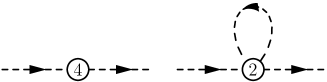
Figure 3.4: Self-energy diagrams at ${\cal O}(p^{4})$. Vertices derived from ${\cal L}_{2n}$ are denoted by $2n$ in the interaction blobs.

For our particular application with exactly two external meson lines, the relevant interaction Lagrangians can be written as

$${\cal L}_{\rm int}={\cal L}_{2}^{4\phi}+{\cal L}_{4}^{2\phi},$$ (3.115)

where ${\cal L}_{2}^{4\phi}$ is given by

$${\cal L}^{4\phi}_{2}=\frac{1}{24F^{2}_{0}}\left\{\mbox{Tr}([\phi,\partial_{\mu}\phi]\phi\partial^{\mu}\phi)+B_{0}\mbox{Tr}(M\phi^{4})\right\}.$$ (3.116)

The terms of ${\cal L}_{4}$ proportional to $L_{9}$, $L_{10}$, $H_{1}$, and $H_{2}$ do not contribute, because they either contain field-strength tensors or external fields only. Since $\partial_{\mu}U={\cal O}(\phi)$, the $L_{1}$, $L_{2}$, and $L_{3}$ terms of Eq. (3.91) are ${\cal O}(\phi^{4})$ and need not be considered. The only candidates are the $L_{4}$ - $L_{8}$ terms, of which we consider the $L_{4}$ term as an explicit example,

$$L_{4}\mbox{Tr}(\partial_{\mu}U\partial^{\mu}U^{\dagger})\mbox{Tr}(\chi U^{\dagger}+U\chi^{\dagger})=$$

$$L_{4}\frac{2}{F_{0}^{2}}[\partial_{\mu}\eta\partial^{\mu}\eta+\partial_{\mu}\pi^{0}\partial^{\mu}\pi^{0}+2\partial_{\mu}\pi^{+}\partial^{\mu}\pi^{-}+2\partial_{\mu}K^{+}\partial^{\mu}K^{-}$$

$$+2\partial_{\mu}K^{0}\partial^{\mu}\bar{K}^{0}+{\cal O}(\phi^{4})][4B_{0}(2m+m_{s})+{\cal O}(\phi^{2})].$$

The remaining terms are treated analogously and we obtain for ${\cal L}_{4}^{2\phi}$

$${\cal L}_{4}^{2\phi} = -\frac{1}{2}\left(a_{\eta}\eta^{2}+b_{\eta}\partial_{\mu}\eta\partial^{\mu}\eta\right)$$ (3.117)

$$-\frac{1}{2}\left(a_{\pi}\pi^{0}\pi^{0}+b_{\pi}\partial_{\mu}\pi^{0}\partial^{\mu}\pi^{0}\right)$$

$$-a_{\pi}\pi^{+}\pi^{-}-b_{\pi}\partial_{\mu}\pi^{+}\partial^{\mu}\pi^{-}$$

$$-a_{K}K^{+}K^{-}-b_{K}\partial_{\mu}K^{+}\partial^{\mu}K^{-}$$

$$-a_{K}K^{0}\bar{K}^{0}-b_{K}\partial_{\mu}K^{0}\partial^{\mu}\bar{K}^{0},$$

where the constants $a_{\phi}$ and $b_{\phi}$ are given by

$$a_{\eta} = \frac{64B^{2}_{0}}{3F^{2}_{0}}\left[(2m+m_{s})(m+2m_{s})L_{6}+2(m-m_{s})^{2}L_{7}+(m^{2}+2m_{s}^{2})L_{8}\right],$$

$$b_{\eta} = -\frac{16B_{0}}{F^{2}_{0}}\left[(2m+m_{s})L_{4}+\frac{1}{3}(m+2m_{s})L_{5}\right],$$

$$a_{\pi} = \frac{64B^{2}_{0}}{F^{2}_{0}}\left[(2m+m_{s})mL_{6}+m^{2}L_{8}\right],$$

$$b_{\pi} = -\frac{16B_{0}}{F^{2}_{0}}\left[(2m+m_{s})L_{4}+mL_{5}\right],$$

$$a_{K} = \frac{32B^{2}_{0}}{F^{2}_{0}}\left[(2m+m_{s})(m+m_{s})L_{6}+\frac{1}{2}(m+m_{s})^{2}L_{8}\right],$$

$$b_{K} = -\frac{16B_{0}}{F^{2}_{0}}\left[(2m+m_{s})L_{4}+\frac{1}{2}(m+m_{s})L_{5}\right].$$ (3.118)

At ${\cal O}(p^{4})$ the self energies are of the form

$$\Sigma_{\phi}(p^{2})=A_{\phi}+B_{\phi}p^{2},$$ (3.119)

where the constants $A_{\phi}$ and $B_{\phi}$ receive a tree-level contribution from ${\cal L}_{4}$ and a one-loop contribution with a vertex from ${\cal L}_{2}$ (see Fig. 3.4). For the tree-level contribution of ${\cal L}_{4}$ this is easily seen, because the Lagrangians of Eq. (3.117) contain either exactly two derivatives of the fields or no derivatives at all. For example, the contact contribution for the $\eta$ reads

$$-i\Sigma_{\eta}^{\rm contact}(p^{2})=i2\left[-\frac{1}{2}a_{\eta}-b_{\eta}\frac{1}{2}(ip_{\mu})(-ip^{\mu})\right]=-i(a_{\eta}+b_{\eta}p^{2}),$$

where, as usual, $\partial_{\mu}\phi$ generates $-ip_{\mu}$ and $ip_{\mu}$ for initial and final lines, respectively, and the factor two takes account of two combinations of contracting the fields with external lines.

For the one-loop contribution the argument is as follows. The Lagrangian ${\cal L}_{2}^{4\phi}$ contains either two derivatives or no derivatives at all which, symbolically, can be written as $\phi\phi\partial\phi\partial\phi$ and $\phi^{4}$, respectively. The first term results in $M^{2}$ or $p^{2}$, depending on whether the $\phi$ or the $\partial\phi$ are contracted with the external fields. The “mixed” situation vanishes upon integration. The second term, $\phi^{4}$, does not generate a momentum dependence.

As a specific example, we evaluate the pion-loop contribution to the $\pi^{0}$ self energy (see Figure 3.5) by applying the Feynman rule of Exercise 3.8.1 for $a=c=3$, $p_{a}=p_{c}=p$, $b=d=j$, and $p_{b}=p_{d}=k$:

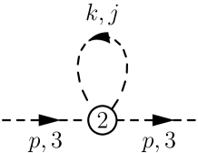
Figure 3.5: Contribution of the pion loops to the $\pi^{0}$ self energy.

$$\frac{1}{2}\int\frac{d^{4}k}{(2\pi)^{4}}i\left[\underbrace{\delta^{3j}\delta^{3j}}_{\mbox{$1$}}\frac{(p+k)^{2}-M_{\pi,2}^{2}}{F_{0}^{2}}+\underbrace{\delta^{33}\delta^{jj}}_{\mbox{$3$}}\frac{-M_{\pi,2}^{2}}{F_{0}^{2}}\right.$$

$$+\underbrace{\delta^{3j}\delta^{j3}}_{\mbox{$1$}}\frac{(p-k)^{2}-M_{\pi,2}^{2}}{F_{0}^{2}}$$

$$\left.-\frac{1}{3F_{0}^{2}}\underbrace{(\delta^{3j}\delta^{3j}+\delta^{33}\delta^{jj}+\delta^{3j}\delta^{j3})}_{\mbox{5}}(2p^{2}+2k^{2}-4M_{\pi,2}^{2})\right]\frac{i}{k^{2}-M_{\pi,2}^{2}+i0^{+}}$$

$$=\frac{1}{2}\int\frac{d^{4}k}{(2\pi)^{4}}\frac{i}{3F_{0}^{2}}[-4p^{2}-4k^{2}+5M^{2}_{\pi,2}]\frac{i}{k^{2}-M_{\pi,2}^{2}+i0^{+}},$$ (3.120)

where $1/2$ is a symmetry factor. The integral of Eq. (3.12) diverges and we thus consider its extension to $n$ dimensions in order to make use of the dimensional-regularization technique described in Section 3.11. In addition to the loop-integral of Eq. (3.107),

$$I(M^{2},\mu^{2},n) = \mu^{4-n}\int\frac{d^{n}k}{(2\pi)^{n}}\frac{i}{k^{2}-M^{2}+i0^{+}}$$ (3.121)

$$= \frac{M^{2}}{16\pi^{2}}\left[R+\ln\left(\frac{M^{2}}{\mu^{2}}\right)\right]+O(n-4),$$

where $R$ is given in Eq. (3.94), we need

$$\mu^{4-n}i\int\frac{d^{n}k}{(2\pi)^{n}}\frac{k^{2}}{k^{2}-M^{2}+i0^{+}}=\mu^{4-n}i\int\frac{d^{n}k}{(2\pi)^{n}}\frac{k^{2}-M^{2}+M^{2}}{k^{2}-M^{2}+i0^{+}},$$

where we have added $0=-M^{2}+M^{2}$ in the numerator. We make use of

$$\mu^{4-n}i\int\frac{d^{n}k}{(2\pi)^{n}}=0$$

in dimensional regularization which is “shown” as follows. Consider the (more general) integral

$$\int d^{n}k(k^{2})^{p},$$ (3.122)

substitute $k=\lambda k^{\prime}\ (\lambda>0)$, and relabel $k^{\prime}=k$

$$=\lambda^{n+2p}\int d^{n}k(k^{2})^{p}.$$

Since $\lambda>0$ is arbitrary and, for fixed $p$, the result is to hold for arbitrary $n$, Eq. (3.122) is set to zero in dimensional regularization. We emphasize that the vanishing of Eq. (3.122) has the character of a prescription. The integral does not depend on any scale and its analytic continuation is ill defined in the sense that there is no dimension $n$ where it is meaningful. It is ultraviolet divergent for $n+2p\geq 0$ and infrared divergent for $n+2p\leq 0$.

We then obtain

$$\mu^{4-n}i\int\frac{d^{n}k}{(2\pi)^{n}}\frac{k^{2}}{k^{2}-M^{2}+i0^{+}}=M^{2}I(M^{2},\mu^{2},n),$$

with $I(M^{2},\mu^{2},n)$ of Eq. (3.121). The pion-loop contribution to the $\pi^{0}$ self energy is thus

$$\frac{i}{6F^{2}_{0}}(-4p^{2}+M^{2}_{\pi,2})I(M^{2}_{\pi,2},\mu^{2},n),$$

which is indeed of the type discussed in Eq. (3.119) and diverges as $n\to 4$.

After analyzing all loop contributions and combining them with the contact contributions of Eqs. (3.12), the constants $A_{\phi}$ and $B_{\phi}$ of Eq. (3.119) are given by

$$A_{\pi} = \frac{M^{2}_{\pi}}{F^{2}_{0}}\Bigg{\{}\underbrace{-\frac{1}{6}I(M^{2}_{\pi})-\frac{1}{6}I(M^{2}_{\eta})-\frac{1}{3}I(M^{2}_{K})}_{\mbox{one-loop contribution}}$$

$$\underbrace{+32[(2m+m_{s})B_{0}L_{6}+mB_{0}L_{8}]}_{\mbox{contact contribution}}\Bigg{\}},$$

$$B_{\pi} = \frac{2}{3}\frac{I(M^{2}_{\pi})}{F^{2}_{0}}+\frac{1}{3}\frac{I(M^{2}_{K})}{F^{2}_{0}}-\frac{16B_{0}}{F^{2}_{0}}\left[(2m+m_{s})L_{4}+mL_{5}\right],$$

$$A_{K} = \frac{M^{2}_{K}}{F^{2}_{0}}\Bigg{\{}\frac{1}{12}I(M^{2}_{\eta})-\frac{1}{4}I(M^{2}_{\pi})-\frac{1}{2}I(M^{2}_{K})$$

$$+32\left[(2m+m_{s})B_{0}L_{6}+\frac{1}{2}(m+m_{s})B_{0}L_{8}\right]\Bigg{\}},$$

$$B_{K} = \frac{1}{4}\frac{I(M^{2}_{\eta})}{F^{2}_{0}}+\frac{1}{4}\frac{I(M^{2}_{\pi})}{F^{2}_{0}}+\frac{1}{2}\frac{I(M^{2}_{K})}{F^{2}_{0}}$$

$$-16\frac{B_{0}}{F^{2}_{0}}\left[(2m+m_{s})L_{4}+\frac{1}{2}(m+m_{s})L_{5}\right],$$

$$A_{\eta} = \frac{M^{2}_{\eta}}{F^{2}_{0}}\left[-\frac{2}{3}I(M^{2}_{\eta})\right]+\frac{M^{2}_{\pi}}{F^{2}_{0}}\left[\frac{1}{6}I(M^{2}_{\eta})-\frac{1}{2}I(M^{2}_{\pi})+\frac{1}{3}I(M^{2}_{K})\right]$$

$$+\frac{M^{2}_{\eta}}{F^{2}_{0}}[16M^{2}_{\eta}L_{8}+32(2m+m_{s})B_{0}L_{6}]$$

$$+\frac{128}{9}\frac{B^{2}_{0}(m-m_{s})^{2}}{F^{2}_{0}}(3L_{7}+L_{8}),$$

$$B_{\eta} = \frac{I(M^{2}_{K})}{F^{2}_{0}}-\frac{16}{F^{2}_{0}}(2m+m_{s})B_{0}L_{4}-8\frac{M^{2}_{\eta}}{F^{2}_{0}}L_{5},$$ (3.123)

where, for simplicity, we have suppressed the dependence on the scale $\mu$ and the number of dimensions $n$ in the integrals $I(M^{2},\mu^{2},n)$ [see Eq. (3.121)]. Furthermore, the squared masses appearing in the loop integrals of Eq. (3.12) are given by the predictions of lowest order, Eqs. (3.54) - (3.56). Finally, the integrals $I$ as well as the bare coefficients $L_{i}$ (with the exception of $L_{7}$) have $1/(n-4)$ poles and finite pieces. In particular, the coefficients $A_{\phi}$ and $B_{\phi}$ are not finite as $n\to 4$.

The masses at ${\cal O}(p^{4})$ are determined by solving the general equation

$$M^{2}=M_{0}^{2}+\Sigma(M^{2})$$ (3.124)

with the predictions of Eq. (3.119) for the self energies,

$$M^{2}=M_{0}^{2}+A+BM^{2},$$

where the lowest-order terms, $M^{2}_{0}$, are given in Eqs. (3.54) - (3.56). We then obtain

$$M^{2}=\frac{M_{0}^{2}+A}{1-B}=M_{0}^{2}(1+B)+A+{\cal O}(p^{6}),$$

because $A={\cal O}(p^{4})$ and $\{B,M_{0}^{2}\}={\cal O}(p^{2})$. Expressing the bare coefficients $L_{i}$ in Eq. (3.12) in terms of the renormalized coefficients by using Eq. (3.92), the results for the masses of the Goldstone bosons at ${\cal O}(p^{4})$ read

$$M^{2}_{\pi,4} = M^{2}_{\pi,2}\Bigg{\{}1+\frac{M^{2}_{\pi,2}}{32\pi^{2}F^{2}_{0}}\ln\left(\frac{M^{2}_{\pi,2}}{\mu^{2}}\right)-\frac{M^{2}_{\eta,2}}{96\pi^{2}F^{2}_{0}}\ln\left(\frac{M^{2}_{\eta,2}}{\mu^{2}}\right)$$ (3.125)

$$+\frac{16}{F^{2}_{0}}\left[(2m+m_{s})B_{0}(2L^{r}_{6}-L^{r}_{4})+mB_{0}(2L^{r}_{8}-L^{r}_{5})\right]\Bigg{\}},$$

$$M^{2}_{K,4} = M^{2}_{K,2}\Bigg{\{}1+\frac{M^{2}_{\eta,2}}{48\pi^{2}F^{2}_{0}}\ln\left(\frac{M^{2}_{\eta,2}}{\mu^{2}}\right)$$

$$+\frac{16}{F^{2}_{0}}\left[(2m+m_{s})B_{0}(2L^{r}_{6}-L^{r}_{4})+\frac{1}{2}(m+m_{s})B_{0}(2L^{r}_{8}-L^{r}_{5})\right]\Bigg{\}},$$

$$M^{2}_{\eta,4} = M^{2}_{\eta,2}\left[1+\frac{M^{2}_{K,2}}{16\pi^{2}F^{2}_{0}}\ln\left(\frac{M^{2}_{K,2}}{\mu^{2}}\right)-\frac{M^{2}_{\eta,2}}{24\pi^{2}F^{2}_{0}}\ln\left(\frac{M^{2}_{\eta,2}}{\mu^{2}}\right)\right.$$ (3.127)

$$\left.+\frac{16}{F^{2}_{0}}(2m+m_{s})B_{0}(2L^{r}_{6}-L^{r}_{4})+8\frac{M^{2}_{\eta,2}}{F^{2}_{0}}(2L^{r}_{8}-L^{r}_{5})\right]$$

$$+M^{2}_{\pi,2}\left[\frac{M^{2}_{\eta,2}}{96\pi^{2}F^{2}_{0}}\ln\left(\frac{M^{2}_{\eta,2}}{\mu^{2}}\right)-\frac{M^{2}_{\pi,2}}{32\pi^{2}F^{2}_{0}}\ln\left(\frac{M^{2}_{\pi,2}}{\mu^{2}}\right)\right.$$

$$\left.+\frac{M^{2}_{K,2}}{48\pi^{2}F^{2}_{0}}\ln\left(\frac{M^{2}_{K,2}}{\mu^{2}}\right)\right]$$

$$+\frac{128}{9}\frac{B^{2}_{0}(m-m_{s})^{2}}{F^{2}_{0}}(3L^{r}_{7}+L^{r}_{8}).$$

In Eqs. (3.125) - (3.127) we have included the subscripts 2 and 4 in order to indicate from which chiral order the predictions result. First of all, we note that the expressions for the masses are finite. The infinite parts of the coefficients $L_{i}$ of the Lagrangian of Gasser and Leutwyler exactly cancel the divergent terms resulting from the integrals. This is the reason why the bare coefficients $L_{i}$ must be infinite. Furthermore, at ${\cal O}(p^{4})$ the masses of the Goldstone bosons vanish, if the quark masses are sent to zero. This is, of course, what we had expected from QCD in the chiral limit but it is comforting to see that the self interaction in ${\cal L}_{2}$ (in the absence of quark masses) does not generate Goldstone boson masses at higher order. The quark masses appear in combination with $B_{0}$ and therefore Eqs. (3.125) - (3.127) (and their generalization for $m_{u}\neq m_{d}$) are used to extract quark mass ratios. At ${\cal O}(p^{4})$, the squared Goldstone boson masses contain terms which are analytic in the quark masses, namely, of the form $m^{2}_{q}$ multiplied by the renormalized low-energy coupling constants $L_{i}^{r}$. However, there are also non-analytic terms of the type $m^{2}_{q}\ln(m_{q})$—so-called chiral logarithms—which do not involve new parameters. Such a behavior is an illustration of the mechanism found by Li and Pagels [Li:1971vr:11], who noticed that a perturbation theory around a symmetry which is realized in the Nambu-Goldstone mode results in both analytic as well as non-analytic expressions in the perturbation. Finally, the scale dependence of the renormalized coefficients $L_{i}^{r}$ of Eq. (3.95) is by construction such that it cancels the scale dependence of the chiral logarithms. Thus, physical observables do not depend on the scale $\mu$. Let us verify this statement by differentiating Eqs. (3.125) - (3.127) with respect to $\mu$. Using Eq. (3.95),

$$L_{i}^{r}(\mu)=L_{i}^{r}(\mu^{\prime})+\frac{\Gamma_{i}}{16\pi^{2}}\ln\left(\frac{\mu^{\prime}}{\mu}\right),$$

we obtain

$$\frac{dL_{i}^{r}(\mu)}{d\mu}=-\frac{\Gamma_{i}}{16\pi^{2}\mu}$$

and, analogously, for the chiral logarithms

$$\frac{d}{d\mu}\ln\left(\frac{M^{2}}{\mu^{2}}\right)=2\frac{d}{d\mu}\left[\ln(M)-\ln(\mu)\right]=-\frac{2}{\mu}.$$

As a specific example, let us differentiate the expression for the pion mass

$$\frac{dM^{2}_{\pi,4}}{d\mu} = \frac{M^{2}_{\pi,2}}{16\pi^{2}\mu F_{0}^{2}}\Bigg{\{}\frac{M^{2}_{\pi,2}}{2}(-2)-\frac{M^{2}_{\eta,2}}{6}(-2)$$

$$+16[(2m+m_{s})B_{0}(-2\Gamma_{6}+\Gamma_{4})+mB_{0}(-2\Gamma_{8}+\Gamma_{5})]\Bigg{\}}$$

$$= \frac{M^{2}_{\pi,2}}{16\pi^{2}\mu F_{0}^{2}}\Bigg{\{}-2B_{0}m+\frac{2}{9}(m+2m_{s})B_{0}$$

$$+16\Bigg{[}(2m+m_{s})B_{0}\underbrace{\left(-2\frac{11}{144}+\frac{1}{8}\right)}_{\mbox{$-\frac{1}{36}$}}+mB_{0}\underbrace{\left(-2\frac{5}{48}+\frac{3}{8}\right)}_{\mbox{$\frac{1}{6}$}}\Bigg{]}\Bigg{\}}$$

$$= \frac{M^{2}_{\pi,2}}{16\pi^{2}\mu F_{0}^{2}}\Bigg{\{}B_{0}m\left(-2+\frac{2}{9}-\frac{8}{9}+\frac{8}{3}\right)+B_{0}m_{s}\left(\frac{4}{9}-\frac{16}{36}\right)\Bigg{\}}$$

$$= 0,$$

where we made use of the $\Gamma_{i}$ of Table 3.3.

Exercise 3.12.1

For the SU(2) calculation of the Goldstone boson self energies at ${\cal O}(p^{4})$ we need the interaction Lagrangian

$${\cal L}_{\rm int}={\cal L}_{2}^{4\phi}+{\cal L}_{4}^{2\phi}.$$

Consider the Lagrangians of Gasser and Leutwyler and of Gasser, Sainio, and Švarc, respectively:

$${\cal L}^{\rm GL}_{4} = \frac{l_{1}}{4}\left\{\mbox{Tr}[D_{\mu}U(D^{\mu}U)^{\dagger}]\right\}^{2}+\frac{l_{2}}{4}\mbox{Tr}[D_{\mu}U(D_{\nu}U)^{\dagger}]\mbox{Tr}[D^{\mu}U(D^{\nu}U)^{\dagger}]$$

$$+\frac{l_{3}}{16}\left[\mbox{Tr}(\chi U^{\dagger}+U\chi^{\dagger})\right]^{2}+\frac{l_{4}}{4}\mbox{Tr}[D_{\mu}U(D^{\mu}\chi)^{\dagger}+D_{\mu}\chi(D^{\mu}U)^{\dagger}]$$

$$+l_{5}\left[\mbox{Tr}(f^{R}_{\mu\nu}Uf^{\mu\nu}_{L}U^{\dagger})-\frac{1}{2}\mbox{Tr}(f_{\mu\nu}^{L}f^{\mu\nu}_{L}+f_{\mu\nu}^{R}f^{\mu\nu}_{R})\right]$$

$$+i\frac{l_{6}}{2}\mbox{Tr}[f^{R}_{\mu\nu}D^{\mu}U(D^{\nu}U)^{\dagger}+f^{L}_{\mu\nu}(D^{\mu}U)^{\dagger}D^{\nu}U]$$

$$-\frac{l_{7}}{16}\left[\mbox{Tr}(\chi U^{\dagger}-U\chi^{\dagger})\right]^{2}$$

$$+\frac{h_{1}+h_{3}}{4}\mbox{Tr}(\chi\chi^{\dagger})+\frac{h_{1}-h_{3}}{16}\left\{\left[\mbox{Tr}(\chi U^{\dagger}+U\chi^{\dagger})\right]^{2}\right.$$

$$\left.+\left[\mbox{Tr}(\chi U^{\dagger}-U\chi^{\dagger})\right]^{2}-2\mbox{Tr}(\chi U^{\dagger}\chi U^{\dagger}+U\chi^{\dagger}U\chi^{\dagger})\right\}$$

$$-2h_{2}\mbox{Tr}(f_{\mu\nu}^{L}f^{\mu\nu}_{L}+f_{\mu\nu}^{R}f^{\mu\nu}_{R}).$$

$${\cal L}^{\rm GSS}_{4} = \frac{l_{1}}{4}\left\{\mbox{Tr}[D_{\mu}U(D^{\mu}U)^{\dagger}]\right\}^{2}+\frac{l_{2}}{4}\mbox{Tr}[D_{\mu}U(D_{\nu}U)^{\dagger}]\mbox{Tr}[D^{\mu}U(D^{\nu}U)^{\dagger}]$$

$$+\frac{l_{3}+l_{4}}{16}\left[\mbox{Tr}(\chi U^{\dagger}+U\chi^{\dagger})\right]^{2}+\frac{l_{4}}{8}\mbox{Tr}[D_{\mu}U(D^{\mu}U)^{\dagger}]\mbox{Tr}(\chi U^{\dagger}+U\chi^{\dagger})$$

$$+l_{5}\mbox{Tr}(f^{R}_{\mu\nu}Uf^{\mu\nu}_{L}U^{\dagger})+i\frac{l_{6}}{2}\mbox{Tr}[f^{R}_{\mu\nu}D^{\mu}U(D^{\nu}U)^{\dagger}+f^{L}_{\mu\nu}(D^{\mu}U)^{\dagger}D^{\nu}U]$$

$$-\frac{l_{7}}{16}\left[\mbox{Tr}(\chi U^{\dagger}-U\chi^{\dagger})\right]^{2}+\frac{h_{1}+h_{3}-l_{4}}{4}\mbox{Tr}(\chi\chi^{\dagger})$$

$$+\frac{h_{1}-h_{3}-l_{4}}{16}\left\{\left[\mbox{Tr}(\chi U^{\dagger}+U\chi^{\dagger})\right]^{2}+\left[\mbox{Tr}(\chi U^{\dagger}-U\chi^{\dagger})\right]^{2}\right.$$

$$\left.-2\mbox{Tr}(\chi U^{\dagger}\chi U^{\dagger}+U\chi^{\dagger}U\chi^{\dagger})\right\}-\frac{4h_{2}+l_{5}}{2}\mbox{Tr}(f_{\mu\nu}^{L}f^{\mu\nu}_{L}+f_{\mu\nu}^{R}f^{\mu\nu}_{R}).$$

Setting the external fields to zero and inserting $\chi=2Bm$, derive the terms involving two pion fields.

Remark: The bare and the renormalized low-energy constants $l_{i}$ and $l_{i}^{r}$ are related by

$$l_{i}=l_{i}^{r}+\gamma_{i}\frac{R}{32\pi^{2}},$$

where $R=2/(n-4)-[\ln(4\pi)+\Gamma^{\prime}(1)+1]$ and

$$\gamma_{1}=\frac{1}{3},\quad\gamma_{2}=\frac{2}{3},\quad\gamma_{3}=-\frac{1}{2},\quad\gamma_{4}=2,\quad\gamma_{5}=-\frac{1}{6},\quad\gamma_{6}=-\frac{1}{3},\quad\gamma_{7}=0.$$

In the SU(2) sector one often uses the scale-independent parameters $\bar{l}_{i}$ which are defined by

$$l_{i}^{r}=\frac{\gamma_{i}}{32\pi^{2}}\left[\bar{l}_{i}+\ln\left(\frac{M^{2}}{\mu^{2}}\right)\right],\quad i=1,\cdots,6,$$

where $M^{2}=B(m_{u}+m_{d})$. Since $\ln(1)=0$, the $\bar{l}_{i}$ are proportional to the renormalized coupling constant at the scale $\mu=M$.

Exercise 3.12.2

Using isospin symmetry, at ${\cal O}(p^{4})$ the pion self energy is of the form

$$\Sigma_{ba}(p^{2})=\delta_{ab}(A+Bp^{2}).$$

The constants $A$ and $B$ receive a tree-level contribution from ${\cal L}_{4}$ and a one-loop contribution from ${\cal L}_{2}$ (see Figure 3.6). Using the results of exercises 3.8.1, 3.11.1, and 3.12.1, derive the expressions of Table 3.4 for the self-energy coefficients.

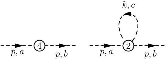
Figure 3.6: Self-energy diagrams at ${\cal O}(p^{4})$. Vertices derived from ${\cal L}_{2n}$ are denoted by $2n$ in the interaction blobs.

	$A$	$B$
GL, exponential	$-\frac{1}{6}\frac{M^{2}}{F^{2}}I+2l_{3}\frac{M^{4}}{F^{2}}$	$\frac{2}{3}\frac{I}{F^{2}}$
GL, square root	$\frac{3}{2}\frac{M^{2}}{F^{2}}I+2l_{3}\frac{M^{4}}{F^{2}}$	$-\frac{I}{F^{2}}$
GSS, exponential	$-\frac{1}{6}\frac{M^{2}}{F^{2}}I+2(l_{3}+l_{4})\frac{M^{4}}{F^{2}}$	$\frac{2}{3}\frac{I}{F^{2}}-2l_{4}\frac{M^{2}}{F^{2}}$
GSS, square root	$\frac{3}{2}\frac{M^{2}}{F^{2}}I+2(l_{3}+l_{4})\frac{M^{4}}{F^{2}}$	$-\frac{I}{F^{2}}-2l_{4}\frac{M^{2}}{F^{2}}$

Table 3.4: Self-energy coefficients and wave function renormalization constants. $I$ denotes the dimensionally regularized integral $I=I(M^{2},\mu^{2},n)=\frac{M^{2}}{16\pi^{2}}\left[R+\ln\left(\frac{M^{2}}{\mu^{2}}\right)\right]+O(n-4)$, $R=\frac{2}{n-4}-\left[\ln(4\pi)+\Gamma^{\prime}(1)+1\right]$, $M^{2}=2Bm$.

Using

$$M^{2}_{\pi,4}=\frac{M^{2}_{\pi,2}+A}{1-B}=M^{2}_{\pi,2}(1+B)+A+{\cal O}(p^{6}),$$

derive the squared pion mass at ${\cal O}(p^{4})$:

$$M_{\pi,4}^{2}=M^{2}-\frac{\bar{l}_{3}}{32\pi^{2}F^{2}}M^{4}+{\cal O}(M^{6}),$$

where $M^{2}=2Bm$.

Exercise 3.12.3

You may repeat the full calculation in SU(3) to obtain the masses of the Goldstone boson octet.

Remark: Conceptionally the calculation is completetly analogous to the SU(2) calculation. Due to the SU(3) algebra and the fact that the loop integrals contain different mass scales it is now considerably more work.

Chapter 4 Chiral Perturbation Theory for Baryons

So far we have considered the purely mesonic sector involving the interaction of Goldstone bosons with each other and with the external fields. However, ChPT can be extended to also describe the dynamics of baryons at low energies. Here we will concentrate on matrix elements with a single baryon in the initial and final states. With such matrix elements we can, e.g., describe static properties such as masses or magnetic moments, form factors, or, finally, more complicated processes, such as pion-nucleon scattering, Compton scattering, pion photoproduction etc. Technically speaking, we are interested in the baryon-to-baryon transition amplitude in the presence of external fields (as opposed to the vacuum-to-vacuum transition amplitude of Section 1.5.3),

$${\cal F}(\vec{p}\,^{\prime},\vec{p};v,a,s,p)=\langle{\vec{p}\,^{\prime}};{\rm out}|{\vec{p}\,};{\rm in}\rangle^{\rm c}_{v,a,s,p},\quad\vec{p}\neq\vec{p}\,^{\prime},$$

determined by the Lagrangian of Eq. (1.183),

$${\cal L}={\cal L}^{0}_{\rm QCD}+{\cal L}_{\rm ext}={\cal L}^{0}_{\rm QCD}+\bar{q}\gamma_{\mu}(v^{\mu}+\frac{1}{3}v^{\mu}_{(s)}+\gamma_{5}a^{\mu})q-\bar{q}(s-i\gamma_{5}p)q.$$

In the above equation $|\vec{p};{\rm in}\rangle$ and $|\vec{p}\,^{\prime};{\rm out}\rangle$ denote asymptotic one-baryon in- and out-states, i.e., states which in the remote past and distant future behave as free one-particle states of momentum $\vec{p}$ and $\vec{p}\,^{\prime}$, respectively. The functional ${\cal F}$ consists of connected diagrams only (superscript c). For example, the matrix elements of the vector and axial-vector currents between one-baryon states are given by

$$\langle\vec{p}\,^{\prime}|V^{\mu,a}(x)|\vec{p}\,\rangle = \left.\frac{\delta}{i\delta v^{a}_{\mu}(x)}{\cal F}(\vec{p}\,^{\prime},\vec{p};v,a,s,p)\right|_{v=0,a=0,s=M,p=0},$$

$$\langle\vec{p}\,^{\prime}|A^{\mu,a}(x)|\vec{p}\,\rangle = \left.\frac{\delta}{i\delta a^{a}_{\mu}(x)}{\cal F}(\vec{p}\,^{\prime},\vec{p};v,a,s,p)\right|_{v=0,a=0,s=M,p=0},$$

where $M=\mbox{diag}(m_{u},m_{d},m_{s})$ denotes the quark-mass matrix and

$$V^{\mu,a}(x)=\bar{q}(x)\gamma^{\mu}\frac{\lambda^{a}}{2}q(x),\quad A^{\mu,a}(x)=\bar{q}(x)\gamma^{\mu}\gamma_{5}\frac{\lambda^{a}}{2}q(x).$$

As in the mesonic sector the method of calculating the Green functions associated with the above functional consists of an effective-Lagrangian approach in combination with an appropriate power counting. Specific matrix elements will be calculated applying the Gell-Mann and Low formula of perturbation theory.

4.1 Transformation Properties of the Fields

The group-theoretical foundations of constructing phenomenological Lagrangians in the presence of spontaneous symmetry breaking have been developed in Refs. [Weinberg:de:1, Coleman:sm:1, Callan:sn:1]. The fields entering the Lagrangian are assumed to transform under irreducible representations of the subgroup $H$ which leaves the vacuum invariant whereas the symmetry group $G$ of the Hamiltonian or Lagrangian is nonlinearly realized (for the transformation behavior of the Goldstone bosons, see Section 3.3).

Our aim is a description of the interaction of baryons with the Goldstone bosons as well as the external fields at low energies. To that end we need to specify the transformation properties of the dynamical fields entering the Lagrangian. Our discussion follows Refs. [Georgi:1, Gasser:1987rb:1].

To be specific, we consider the octet of the $\frac{1}{2}^{+}$ baryons (see Figure 4.1). With each member of the octet we associate a complex, four-component Dirac field which we arrange in a traceless $3\times 3$ matrix $B$,

Figure 4.1: The baryon octet in an $(I_{3},S)$ diagram. We have included the masses in MeV as well as the quark content.

$$B=\sum_{a=1}^{8}\frac{\lambda_{a}B_{a}}{\sqrt{2}}=\left(\begin{array}[]{ccc}\frac{1}{\sqrt{2}}\Sigma^{0}+\frac{1}{\sqrt{6}}\Lambda&\Sigma^{+}&p\\ \Sigma^{-}&-\frac{1}{\sqrt{2}}\Sigma^{0}+\frac{1}{\sqrt{6}}\Lambda&n\\ \Xi^{-}&\Xi^{0}&-\frac{2}{\sqrt{6}}\Lambda\end{array}\right),$$ (4.1)

where we have suppressed the dependence on $x$. For later use, we have to keep in mind that each entry of Eq. (4.1) is a Dirac field, but for the purpose of discussing the transformation properties under global flavor SU(3) this can be ignored, because these transformations act on each of the four components in the same way. In contrast to the mesonic case of Eq. (3.4), where we collected the fields of the Goldstone octet in a Hermitian traceless matrix $\phi$, the $B_{a}$ of the spin-$1/2$ case are not real (Hermitian), i.e., $B\neq B^{\dagger}$.

Exercise 4.1.1

Using Eq. (4.1), express the physical fields in terms of Cartesian fields.

Now let us define the set

$$M\equiv\{B(x)|B(x)\,\mbox{complex, traceless $3\times 3$ matrix}\}$$ (4.2)

which under the addition of matrices is a complex vector space. The following homomorphism is a representation of the abstract group $H=\mbox{SU}(3)_{V}$ on the vector space $M$ [see also Eq. (3.31)]:

$$\varphi:H\to\varphi(H),\quad V\mapsto\varphi(V)\quad\mbox{where}\quad\varphi(V):M\to M,$$

$$B(x)\mapsto B^{\prime}(x)=\varphi(V)B(x)\equiv VB(x)V^{\dagger}.$$ (4.3)

First of all, $B^{\prime}(x)$ is again an element of $M$, because $\mbox{Tr}[B^{\prime}(x)]=\mbox{Tr}[VB(x)V^{\dagger}]\newline =\mbox{Tr}[B(x)]=0$. Equation (4.1) satisfies the homomorphism property

$$\varphi(V_{1})\varphi(V_{2})B(x) = \varphi(V_{1})V_{2}B(x)V_{2}^{\dagger}=V_{1}V_{2}B(x)V_{2}^{\dagger}V_{1}^{\dagger}=(V_{1}V_{2})B(x)(V_{1}V_{2})^{\dagger}$$

$$= \varphi(V_{1}V_{2})B(x)$$

and is indeed a representation of SU(3), because

$$\varphi(V)[\lambda_{1}B_{1}(x)+\lambda_{2}B_{2}(x)] = V[\lambda_{1}B_{1}(x)+\lambda_{2}B_{2}(x)]V^{\dagger}$$

$$= \lambda_{1}VB_{1}(x)V^{\dagger}+\lambda_{2}VB_{2}(x)V^{\dagger}$$

$$= \lambda_{1}\varphi(V)B_{1}(x)+\lambda_{2}\varphi(V)B_{2}(x).$$

Equation (4.1) is just the familiar statement that $B$ transforms as an octet under (the adjoint representation of) SU(3)_V.

Let us now turn to various representations and realizations of the group $\mbox{SU(3)}_{L}\times\mbox{SU(3)}_{R}$. We consider two explicit examples and refer the interested reader to the textbook by Georgi [Georgi:1] for more details. In analogy to the discussion of the quark fields in QCD, we may introduce left- and right-handed components of the baryon fields [see Eq. (1.55)]:

$$B_{1}=P_{L}B_{1}+P_{R}B_{1}=B_{L}+B_{R}.$$ (4.4)

We define the set $M_{1}\equiv\{(B_{L}(x),B_{R}(x))\}$ which under the addition of matrices is a complex vector space. The following homomorphism is a representation of the abstract group $G=\mbox{SU}(3)_{L}\times\mbox{SU(3)}_{R}$ on $M_{1}$:

$$(B_{L},B_{R})\mapsto(B^{\prime}_{L},B^{\prime}_{R})\equiv(LB_{L}L^{\dagger},RB_{R}R^{\dagger}),$$ (4.5)

where we have suppressed the $x$ dependence. The proof proceeds in complete analogy to that of Eq. (4.1).

As a second example, consider the set $M_{2}\equiv\{B_{2}(x)\}$ with the homomorphism

$$B_{2}\mapsto B_{2}^{\prime}\equiv LB_{2}L^{\dagger},$$ (4.6)

i.e. the transformation behavior is independent of $R$. The mapping defines a representation of the group $\mbox{SU(3)}_{L}\times\mbox{SU(3)}_{R}$, although the transformation behavior is drastically different from the first example. However, the important feature which both mappings have in common is that under the subgroup $H=\{(V,V)|V\in\mbox{SU($3$)}\}$ of $G$ both fields $B_{i}$ transform as an octet:

$$B_{1}=B_{L}+B_{R} \stackrel{{\scriptstyle H}}{{\mapsto}} VB_{L}V^{\dagger}+VB_{R}V^{\dagger}=VB_{1}V^{\dagger},$$

$$B_{2} \stackrel{{\scriptstyle H}}{{\mapsto}} VB_{2}V^{\dagger}.$$

We will now show how in a theory also containing Goldstone bosons the various realizations may be connected to each other using field redefinitions. Here we consider the second example, with the fields $B_{2}$ of Eq. (4.6) and $U$ of Eq. (3.4) transforming as

$$B_{2}\mapsto LB_{2}L^{\dagger},\quad U\mapsto RUL^{\dagger},$$

and define new baryon fields by

$$\tilde{B}\equiv UB_{2},$$

so that the new pair $(\tilde{B},U)$ transforms as

$$\tilde{B}\mapsto RUL^{\dagger}LB_{2}L^{\dagger}=R\tilde{B}L^{\dagger},\quad U\mapsto RUL^{\dagger}.$$

Note in particular that $\tilde{B}$ still transforms as an octet under the subgroup $H=\mbox{SU(3)}_{V}$.

Given that physical observables are invariant under field transformations we may choose a description of baryons that is maximally convenient for the construction of the effective Lagrangian [Georgi:1] and which is commonly used in chiral perturbation theory. We start with $G=\mbox{SU(2)}_{L}\times\mbox{SU(2)}_{R}$ and consider the case of $G=\mbox{SU(3)}_{L}\times\mbox{SU(3)}_{R}$ later. Let

$$\Psi=\left(\begin{array}[]{c}p\\ n\end{array}\right)$$ (4.7)

denote the nucleon field with two four-component Dirac fields for the proton and the neutron and $U$ the SU(2) matrix containing the pion fields. We have already seen in Section 3.3.2 that the mapping $U\mapsto RUL^{\dagger}$ defines a nonlinear realization of $G$. We denote the square root of $U$ by $u$, $u^{2}(x)=U(x)$, and define the SU(2)-valued function $K(L,R,U)$ by

$$u(x)\mapsto u^{\prime}(x)=\sqrt{RUL^{\dagger}}\equiv RuK^{-1}(L,R,U),$$ (4.8)

i.e.

$$K(L,R,U)=u^{\prime-1}Ru=\sqrt{RUL^{\dagger}}^{-1}R\sqrt{U}.$$

The following homomorphism defines an operation of $G$ on the set $\{(U,\Psi)\}$ in terms of a nonlinear realization:

$$\varphi(g):\left(\begin{array}[]{c}U\\ \Psi\end{array}\right)\mapsto\left(\begin{array}[]{c}U^{\prime}\\ \Psi^{\prime}\end{array}\right)=\left(\begin{array}[]{c}RUL^{\dagger}\\ K(L,R,U)\Psi\end{array}\right),$$ (4.9)

because the identity leaves $(U,\Psi)$ invariant and

$$\varphi(g_{1})\varphi(g_{2})\left(\begin{array}[]{c}U\\ \Psi\end{array}\right) = \varphi(g_{1})\left(\begin{array}[]{c}R_{2}UL_{2}^{\dagger}\\ K(L_{2},R_{2},U)\Psi\end{array}\right)$$

$$= \left(\begin{array}[]{c}R_{1}R_{2}UL_{2}^{\dagger}L_{1}^{\dagger}\\ K(L_{1},R_{1},R_{2}UL_{2}^{\dagger})K(L_{2},R_{2},U)\Psi\end{array}\right)$$

$$= \left(\begin{array}[]{c}R_{1}R_{2}U(L_{1}L_{2})^{\dagger}\\ K(L_{1}L_{2},R_{1}R_{2},U)\Psi\end{array}\right)$$

$$= \varphi(g_{1}g_{2})\left(\begin{array}[]{c}U\\ \Psi\end{array}\right).$$

Exercise 4.1.2

Consider the SU(3)-valued function

$$K(L,R,U)=\sqrt{RUL^{\dagger}}^{-1}R\sqrt{U}.$$

Verify the homomorphism property

$$K(L_{1},R_{1},R_{2}UL_{2}^{\dagger})K(L_{2},R_{2},U)=K((L_{1}L_{2}),(R_{1}R_{2}),U).$$

Note that for a general group element $g=(L,R)$ the transformation behavior of $\Psi$ depends on $U$. For the special case of an isospin transformation, $R=L=V$, one obtains $u^{\prime}=VuV^{\dagger}$, because

$$U^{\prime}=u^{\prime 2}=VuV^{\dagger}VuV^{\dagger}=Vu^{2}V^{\dagger}=VUV^{\dagger}.$$

Comparing with Eq. (4.8) yields $K^{-1}(V,V,U)=V^{\dagger}$ or $K(V,V,U)=V$, i.e., $\Psi$ transforms linearly as an isospin doublet under the isospin subgroup $\mbox{SU(2)}_{V}$ of $\mbox{SU(2)}_{L}\times\mbox{SU(2)}_{R}$. A general feature here is that the transformation behavior under the subgroup which leaves the ground state invariant is independent of $U$. Moreover, as already discussed in Section 3.3.2, the Goldstone bosons $\phi$ transform according to the adjoint representation of SU(2)_V, i.e., as an isospin triplet.

For the case $G=\mbox{SU(3)}_{L}\times\mbox{SU(3)}_{R}$ one uses the nonlinear realization

$$\varphi(g):\left(\begin{array}[]{c}U\\ B\end{array}\right)\mapsto\left(\begin{array}[]{c}U^{\prime}\\ B^{\prime}\end{array}\right)=\left(\begin{array}[]{c}RUL^{\dagger}\\ K(L,R,U)BK^{\dagger}(L,R,U)\end{array}\right),$$ (4.14)

where $K$ is defined completely analogously to Eq. (4.8) after inserting the corresponding SU(3) matrices.

4.2 Baryonic Effective Lagrangian at Lowest Order

Given the dynamical fields of Eqs. (4.9) and (4.14) and their transformation properties, we will now discuss the most general effective baryonic Lagrangian at lowest order. As in the vacuum sector, chiral symmetry provides constraints among the single-baryon Green functions. Analogous to the mesonic sector, these Ward identities will be satisfied if the Green functions are calculated from the most general effective Lagrangian coupled to external fields with a local invariance under the chiral group (see Section 1.4).

Let us start with the construction of the $\pi N$ effective Lagrangian ${\cal L}^{(1)}_{\pi N}$ which we demand to have a local $\mbox{SU}(2)_{L}\times\mbox{SU(2)}_{R}\times\mbox{U(1)}_{V}$ symmetry. The transformation behavior of the external fields is given in Eq. (1.5.3), whereas the nucleon doublet and $U$ transform as

$$\left(\begin{array}[]{c}U(x)\\ \Psi(x)\end{array}\right)\mapsto\left(\begin{array}[]{c}V_{R}(x)U(x)V_{L}^{\dagger}(x)\\ \exp[-i\Theta(x)]K[V_{L}(x),V_{R}(x),U(x)]\Psi(x)\end{array}\right).$$ (4.15)

The local character of the transformation implies that we need to introduce a covariant derivative $D_{\mu}\Psi$ with the usual property that it transforms in the same way as $\Psi$:

$$D_{\mu}\Psi(x)\mapsto[D_{\mu}\Psi(x)]^{\prime}\stackrel{{\scriptstyle!}}{{=}}\exp[-i\Theta(x)]K[V_{L}(x),V_{R}(x),U(x)]D_{\mu}\Psi(x).$$ (4.16)

Since $K$ not only depends on $V_{L}$ and $V_{R}$ but also on $U$, we may expect the covariant derivative to contain $u$ and $u^{\dagger}$ and their derivatives.

The so-called connection (recall $\partial_{\mu}uu^{\dagger}=-u\partial_{\mu}u^{\dagger}$),

$$\Gamma_{\mu}=\frac{1}{2}\left[u^{\dagger}(\partial_{\mu}-ir_{\mu})u+u(\partial_{\mu}-il_{\mu})u^{\dagger}\right],$$ (4.17)

is an integral part of the covariant derivative of the nucleon doublet:

$$D_{\mu}\Psi=(\partial_{\mu}+\Gamma_{\mu}-iv_{\mu}^{(s)})\Psi.$$ (4.18)

What needs to be shown is

$$D^{\prime}_{\mu}\Psi^{\prime}=[\partial_{\mu}+\Gamma_{\mu}^{\prime}-i(v_{\mu}^{(s)}-\partial_{\mu}\Theta)]\exp(-i\Theta)K\Psi=\exp(-i\Theta)K(\partial_{\mu}+\Gamma_{\mu}-iv_{\mu}^{(s)})\Psi.$$ (4.19)

To that end, we make use of the product rule,

$$\partial_{\mu}[\exp(-i\Theta)K\Psi]=-i\partial_{\mu}\Theta\exp(-i\Theta)K\Psi+\exp(-i\Theta)\partial_{\mu}K\Psi+\exp(-i\Theta)K\partial_{\mu}\Psi,$$

in Eq. (4.19) and multiply by $\exp(i\Theta)$, reducing it to

$$\partial_{\mu}K=K\Gamma_{\mu}-\Gamma_{\mu}^{\prime}K.$$

Using Eq. (4.8),

$$K = u^{\prime\dagger}V_{R}u=\underbrace{u^{\prime}u^{\prime\dagger}}_{\mbox{1}}u^{\prime\dagger}V_{R}u=u^{\prime}U^{\prime\dagger}V_{R}u=u^{\prime}V_{L}\underbrace{U^{\dagger}}_{\mbox{$u^{\dagger}u^{\dagger}$}}\underbrace{V_{R}^{\dagger}V_{R}}_{\mbox{1}}u=u^{\prime}V_{L}u^{\dagger},$$

we find

$$2(K\Gamma_{\mu}-\Gamma_{\mu}^{\prime}K) = K\left[u^{\dagger}(\partial_{\mu}-ir_{\mu})u\right]-\left[u^{\prime\dagger}(\partial_{\mu}-iV_{R}r_{\mu}V_{R}^{\dagger}+V_{R}\partial_{\mu}V_{R}^{\dagger})u^{\prime}\right]K$$

$$+(R\to L,r_{\mu}\to l_{\mu},u\leftrightarrow u^{\dagger},u^{\prime}\leftrightarrow u^{\prime\dagger})$$

$$= u^{\prime\dagger}V_{R}(\partial_{\mu}u-ir_{\mu}u)-u^{\prime\dagger}\partial_{\mu}u^{\prime}\underbrace{K}_{\mbox{$u^{\prime\dagger}V_{R}u$}}$$

$$+iu^{\prime\dagger}V_{R}r_{\mu}\underbrace{V_{R}^{\dagger}u^{\prime}K}_{\mbox{$u$}}-u^{\prime\dagger}V_{R}\partial_{\mu}V^{\dagger}_{R}\underbrace{u^{\prime}K}_{\mbox{$V_{R}u$}}$$

$$+(R\to L,r_{\mu}\to l_{\mu},u\leftrightarrow u^{\dagger},u^{\prime}\leftrightarrow u^{\prime\dagger})$$

$$= u^{\prime\dagger}V_{R}\partial_{\mu}u-iu^{\prime\dagger}V_{R}r_{\mu}u-\underbrace{u^{\prime\dagger}\partial_{\mu}u^{\prime}u^{\prime\dagger}}_{\mbox{$-\partial_{\mu}u^{\prime\dagger}$}}V_{R}u$$

$$+iu^{\prime\dagger}V_{R}r_{\mu}u-u^{\prime\dagger}\underbrace{V_{R}\partial_{\mu}V_{R}^{\dagger}V_{R}}_{\mbox{$-\partial_{\mu}V_{R}$}}u$$

$$+(R\to L,r_{\mu}\to l_{\mu},u\leftrightarrow u^{\dagger},u^{\prime}\leftrightarrow u^{\prime\dagger})$$

$$= u^{\prime\dagger}V_{R}\partial_{\mu}u+\partial_{\mu}u^{\prime\dagger}V_{R}u+u^{\prime\dagger}\partial_{\mu}V_{R}u$$

$$+(R\to L,u\leftrightarrow u^{\dagger},u^{\prime}\leftrightarrow u^{\prime\dagger})$$

$$= \partial_{\mu}(u^{\prime\dagger}V_{R}u+u^{\prime}V_{L}u^{\dagger})=2\partial_{\mu}K,$$

i.e., the covariant derivative defined in Eq. (4.18) indeed satisfies the condition of Eq. (4.16). At ${\cal O}(p)$ there exists another Hermitian building block, the so-called vielbein,

$$u_{\mu}\equiv i\left[u^{\dagger}(\partial_{\mu}-ir_{\mu})u-u(\partial_{\mu}-il_{\mu})u^{\dagger}\right],$$ (4.20)

which under parity transforms as an axial vector:

$$u_{\mu}\stackrel{{\scriptstyle P}}{{\mapsto}}i\left[u(\partial^{\mu}-il^{\mu})u^{\dagger}-u^{\dagger}(\partial^{\mu}-ir^{\mu})u\right]=-u^{\mu}.$$

Exercise 4.2.1

Using

$$u^{\prime}=V_{R}uK^{\dagger}=KuV_{L}^{\dagger}$$

show that, under $\mbox{SU(2)}_{L}\times\mbox{SU(2)}_{R}\times\mbox{U}(1)_{V}$, $u_{\mu}$ transforms as

$$u_{\mu}\mapsto Ku_{\mu}K^{\dagger}.$$

The most general effective $\pi N$ Lagrangian describing processes with a single nucleon in the initial and final states is then of the type $\bar{\Psi}\widehat{O}\Psi$, where $\widehat{O}$ is an operator acting in Dirac and flavor space, transforming under $\mbox{SU(2)}_{L}\times\mbox{SU(2)}_{R}\times\mbox{U}(1)_{V}$ as $K\widehat{O}K^{\dagger}$. As in the mesonic sector, the Lagrangian must be a Hermitian Lorentz scalar which is even under the discrete symmetries $C$, $P$, and $T$.

The most general such Lagrangian with the smallest number of derivatives is given by [Gasser:1987rb:2]

$${\cal L}^{(1)}_{\pi N}=\bar{\Psi}\left(iD/-\stackrel{{\scriptstyle\circ}}{{m}}_{N}+\frac{\stackrel{{\scriptstyle\circ}}{{g}}_{A}}{2}\gamma^{\mu}\gamma_{5}u_{\mu}\right)\Psi.$$ (4.21)

It contains two parameters not determined by chiral symmetry: the nucleon mass $\stackrel{{\scriptstyle\circ}}{{m}}_{N}$ and the axial-vector coupling constant $\stackrel{{\scriptstyle\circ}}{{g}}_{A}$, both taken in the chiral limit (denoted by $\circ$). [Physical nucleon mass: $m_{N}=939$ MeV. Theoretical analysis: $\stackrel{{\scriptstyle\circ}}{{m}}_{N}\approx 883$ MeV (at fixed $m_{s}\neq 0$). Physical axial-vector coupling constant from neutron beta decay: $g_{A}=1.267$.] The overall normalization of the Lagrangian is chosen such that in the case of no external fields and no pion fields it reduces to that of a free nucleon of mass $\stackrel{{\scriptstyle\circ}}{{m}}_{N}$.

Exercise 4.2.2

Consider the lowest-order $\pi N$ Lagrangian of Eq. (4.21). Assume that there are no external fields, $l_{\mu}=r_{\mu}=v_{\mu}^{(s)}=0$, so that

$$\Gamma_{\mu} = \frac{1}{2}(u^{\dagger}\partial_{\mu}u+u\partial_{\mu}u^{\dagger}),$$

$$u_{\mu} = i(u^{\dagger}\partial_{\mu}u-u\partial_{\mu}u^{\dagger}).$$

By expanding

$$u=\exp\left(i\frac{\vec{\tau}\cdot\vec{\phi}}{2F}\right)=1+i\frac{\vec{\tau}\cdot\vec{\phi}}{2F}-\frac{\vec{\phi}\,^{2}}{8F^{2}}+\cdots,$$

derive the interaction Lagrangians containing one and two pion fields, respectively.

Exercise 4.2.3

Consider the two-flavor Lagrangian

$${\cal L}_{\rm eff}={\cal L}^{(1)}_{\pi N}+{\cal L}_{2}^{\pi},$$

where

$${\cal L}^{(1)}_{\pi N} = \bar{\Psi}\left(iD/-\stackrel{{\scriptstyle\circ}}{{m}}_{N}+\frac{\stackrel{{\scriptstyle\circ}}{{g}}_{A}}{2}\gamma^{\mu}\gamma_{5}u_{\mu}\right)\Psi,$$

$${\cal L}_{2}^{\pi} = \frac{F^{2}}{4}\mbox{Tr}[D_{\mu}U(D^{\mu}U)^{\dagger}]+\frac{F^{2}}{4}\mbox{Tr}(\chi U^{\dagger}+U\chi^{\dagger}).$$

1. We would like to study this Lagrangian in the presence of an electromagnetic field ${\cal A}_{\mu}$. For that purpose we need to insert for the external fields

   $$r_{\mu}=l_{\mu}=-e\frac{\tau_{3}}{2}{\cal A}_{\mu},\quad v_{\mu}^{(s)}=-\frac{e}{2}{\cal A}_{\mu}.$$

   Derive the interaction Lagrangians ${\cal L}_{\gamma NN}$, ${\cal L}_{\pi NN}$, ${\cal L}_{\gamma\pi NN}$, and ${\cal L}_{\gamma\pi\pi}$. Here, the nomenclature is such that ${\cal L}_{\gamma NN}$ denotes the interaction Lagrangian describing the interaction of an external electromagnetic field with a single nucleon in the initial and final states, respectively. For example, ${\cal L}_{\gamma\pi NN}$ must be symbolically of the type $\bar{\Psi}\phi{\cal A}\Psi$. Using Feynman rules, these four interaction Lagrangians would be sufficient to describe pion photoproduction of the nucleon, $\gamma N\to\pi N$, at lowest order in ChPT.

2. Now we would like to describe the interaction with a massive charged weak boson ${\cal W}^{\pm}_{\mu}=({\cal W}_{1\mu}\mp i{\cal W}_{2\mu})/\sqrt{2}$,

   $$r_{\mu}=0,\quad l_{\mu}=-\frac{g}{\sqrt{2}}({\cal W}^{+}_{\mu}T_{+}+\mbox{H.c.}),$$

   where H.c. refers to the Hermitian conjugate and

   $$T_{+}=\left(\begin{array}[]{rr}0&V_{ud}\\ 0&0\end{array}\right).$$

   Here, $V_{ud}$ denotes an element of the Cabibbo-Kobayashi-Maskawa quark-mixing matrix,

   $$|V_{ud}|=0.9735\pm 0.0008.$$

   At lowest order in perturbation theory, the Fermi constant is related to the gauge coupling $g$ and the $W$ mass as

   $$G_{F}=\sqrt{2}\frac{g^{2}}{8M^{2}_{W}}=1.16639(1)\times 10^{-5}\,\mbox{GeV}^{-2}.$$

   Derive the interaction Lagrangians ${\cal L}_{WNN}$ and ${\cal L}_{W\pi}$.

3. Finally, we consider the neutral weak interaction

   $$r_{\mu} = e\tan(\theta_{W})\frac{\tau_{3}}{2}{\cal Z}_{\mu},$$

   $$l_{\mu} = -\frac{g}{\cos(\theta_{W})}\frac{\tau_{3}}{2}{\cal Z}_{\mu}+e\tan(\theta_{W})\frac{\tau_{3}}{2}{\cal Z}_{\mu},$$

   $$v_{\mu}^{(s)} = \frac{e\tan(\theta_{W})}{2}{\cal Z}_{\mu},$$

   where $\theta_{W}$ is the weak angle, $e=g\sin(\theta_{W})$. Derive the interaction Lagrangians ${\cal L}_{ZNN}$ and ${\cal L}_{Z\pi}$.

Since the nucleon mass $m_{N}$ does not vanish in the chiral limit, the zeroth component $\partial^{0}$ of the partial derivative acting on the nucleon field does not produce a “small” quantity. We thus have to address the new features of chiral power counting in the baryonic sector. The counting of the external fields as well as of covariant derivatives acting on the mesonic fields remains the same as in mesonic chiral perturbation theory [see Eq. (3.70) of Section 3.6]. On the other hand, the counting of bilinears $\bar{\Psi}\Gamma\Psi$ is probably easiest understood by investigating the matrix elements of positive-energy plane-wave solutions to the free Dirac equation in the Dirac representation:

$$\psi^{(+)}(\vec{x},t)=\exp(-ip_{N}\cdot x)\sqrt{E_{N}+m_{N}}\left(\begin{array}[]{c}\chi\\ \frac{\vec{\sigma}\cdot\vec{p}_{N}}{E_{N}+m_{N}}\chi\end{array}\right),$$ (4.22)

where $\chi$ denotes a two-component Pauli spinor and $p_{N}^{\mu}=(E_{N},\vec{p}_{N})$ with $E_{N}=\sqrt{\vec{p}\,_{N}^{2}+m_{N}^{2}}$. In the low-energy limit, i.e. for nonrelativistic kinematics, the lower (small) component is suppressed as $|\vec{p}_{N}|/m_{N}$ in comparison with the upper (large) component. For the analysis of the bilinears it is convenient to divide the 16 Dirac matrices into even and odd ones, ${\cal E}=\{1,\gamma_{0},\gamma_{5}\gamma_{i},\sigma_{ij}\}$ and ${\cal O}=\{\gamma_{5},\gamma_{5}\gamma_{0},\gamma_{i},\sigma_{i0}\}$ [Foldy:1949wa:2, Fearing:ii:2], respectively, where odd matrices couple large and small components but not large with large, whereas even matrices do the opposite. Finally, $i\partial^{\mu}$ acting on the nucleon solution produces $p_{N}^{\mu}$ which we write symbolically as $p_{N}^{\mu}=(m_{N},\vec{0})+(E_{N}-m_{N},\vec{p}_{N}\,)$ where we count the second term as ${\cal O}(p)$, i.e., as a small quantity. We are now in the position to summarize the chiral counting scheme for the (new) elements of baryon chiral perturbation theory [Krause:xc:2]:

$$\Psi,\bar{\Psi}={\cal O}(p^{0}),\,D_{\mu}\Psi={\cal O}(p^{0}),\,(iD/-\stackrel{{\scriptstyle\circ}}{{m}}_{N})\Psi={\cal O}(p),$$

$$1,\gamma_{\mu},\gamma_{5}\gamma_{\mu},\sigma_{\mu\nu}={\cal O}(p^{0}),\,\gamma_{5}={\cal O}(p),$$ (4.23)

where the order given is the minimal one. For example, $\gamma_{\mu}$ has both an ${\cal O}(p^{0})$ piece, $\gamma_{0}$, as well as an ${\cal O}(p)$ piece, $\gamma_{i}$. A rigorous nonrelativistic reduction may be achieved in the framework of the Foldy-Wouthuysen method [Foldy:1949wa:2, Fearing:ii:2] or the heavy-baryon approach [Jenkins:1990jv:2, Bernard:1992qa:2].

The construction of the $\mbox{SU(3)}_{L}\times\mbox{SU(3)}_{R}$ Lagrangian proceeds similarly except for the fact that the baryon fields are contained in the $3\times 3$ matrix of Eq. (4.1) transforming as $KBK^{\dagger}$. As in the mesonic sector, the building blocks are written as products transforming as $K\cdots K^{\dagger}$ with a trace taken at the end. The lowest-order Lagrangian reads [Krause:xc:2, Georgi:2]

$${\cal L}^{(1)}_{MB}=\mbox{Tr}\left[\bar{B}\left(iD/\hskip 1.99997pt-M_{0}\right)B\right]-\frac{D}{2}\mbox{Tr}\left(\bar{B}\gamma^{\mu}\gamma_{5}\{u_{\mu},B\}\right)-\frac{F}{2}\mbox{Tr}\left(\bar{B}\gamma^{\mu}\gamma_{5}[u_{\mu},B]\right),$$ (4.24)

where $M_{0}$ denotes the mass of the baryon octet in the chiral limit. The covariant derivative of $B$ is defined as

$$D_{\mu}B=\partial_{\mu}B+[\Gamma_{\mu},B],$$ (4.25)

with $\Gamma_{\mu}$ of Eq. (4.17) [for $\mbox{SU(3)}_{L}\times\mbox{ SU(3)}_{R}$]. The constants $D$ and $F$ may be determined by fitting the semi-leptonic decays $B\to B^{\prime}+e^{-}+\bar{\nu}_{e}$ at tree level [Borasoy:1998pe:2]:

$$D=0.80,\quad F=0.50.$$ (4.26)

Other “popular” values are: ($D=0.75$, $F=0.5$), ($D=0.804$, $F=0.463$).

Exercise 4.2.4

Consider the three-flavor Lagrangian of Eq. (4.24) in the absence of external fields:

$$D_{\mu}B = \partial_{\mu}B+\frac{1}{2}[u^{\dagger}\partial_{\mu}u+u\partial_{\mu}u^{\dagger},B],$$

$$u_{\mu} = i(u^{\dagger}\partial_{\mu}u-u\partial_{\mu}u^{\dagger}).$$

Using

$$B=\frac{B_{a}\lambda_{a}}{\sqrt{2}},\quad\bar{B}=\frac{\bar{B}_{b}\lambda_{b}}{\sqrt{2}},$$

show that the interaction Lagrangians with one and two mesons can be written as

$${\cal L}^{(1)}_{\phi BB} = \frac{1}{F_{0}}(d_{abc}D+if_{abc}F)\bar{B}_{b}\gamma^{\mu}\gamma_{5}B_{a}\partial_{\mu}\phi_{c},$$

$${\cal L}^{(1)}_{\phi\phi BB} = -\frac{i}{2F_{0}^{2}}f_{abe}f_{cde}\bar{B}_{b}\gamma^{\mu}B_{a}\phi_{c}\partial_{\mu}\phi_{d}.$$

Hint: $u^{\dagger}\partial_{\mu}u+u\partial_{\mu}u^{\dagger}=u^{\dagger}\partial_{\mu}u-\partial_{\mu}uu^{\dagger}=[u^{\dagger},\partial_{\mu}u]$.

4.3 Application at Lowest Order: Goldberger-Treiman Relation and the Axial-Vector Current Matrix Element

We have seen in Section 1.3.6 that the quark masses in QCD give rise to a non-vanishing divergence of the axial-vector current operator [see Eq. (1.3.6)]. Here we will discuss the implications for the matrix elements of the pseudoscalar density and of the axial-vector current evaluated between single-nucleon states in terms of the lowest-order Lagrangians of Eqs. (3.78) and (4.21). In particular, we will see that the Ward identity

$$\langle N(p^{\prime})|\partial_{\mu}A^{\mu}_{i}(0)|N(p)\rangle=\langle N(p^{\prime})|m_{q}P_{i}(0)|N(p)\rangle,$$ (4.27)

where $m_{q}=m_{u}=m_{d}$, is satisfied.

The nucleon matrix element of the pseudoscalar density can be parameterized as

$$m_{q}\langle N(p^{\prime})|P_{i}(0)|N(p)\rangle=\frac{M_{\pi}^{2}F_{\pi}}{M_{\pi}^{2}-t}G_{\pi N}(t)i\bar{u}(p^{\prime})\gamma_{5}\tau_{i}u(p),$$ (4.28)

where $t=(p^{\prime}-p)^{2}$. Equation (4.28) defines the form factor $G_{\pi N}(t)$ in terms of the QCD operator $m_{q}P_{i}(x)$. The operator $m_{q}P_{i}(x)/(M_{\pi}^{2}F_{\pi})$ serves as an interpolating pion field and thus $G_{\pi N}(t)$ is also referred to as the pion-nucleon form factor (for this specific choice of the interpolating pion field). The pion-nucleon coupling constant $g_{\pi N}$ is defined through $G_{\pi N}(t)$ evaluated at $t=M_{\pi}^{2}$.

The Lagrangian ${\cal L}_{\pi N}^{(1)}$ of Eq. (4.21) does not generate a direct coupling of an external pseudoscalar field $p_{i}(x)$ to the nucleon, i.e., it does not contain any terms involving $\chi$ or $\chi^{\dagger}$. At lowest order in the chiral expansion, the matrix element of the pseudoscalar density is therefore given in terms of the diagram of Figure 4.2, i.e., the pseudoscalar source produces a pion which propagates and is then absorbed by the nucleon.

Figure 4.2: Lowest-order contribution to the single-nucleon matrix element of the pseudoscalar density. Mesonic and baryonic vertices are denoted by a circle and a box, respectively, with the numbers 2 and 1 referring to the chiral order of ${\cal L}_{2}$ and ${\cal L}^{(1)}_{\pi N}$.

The coupling of a pseudoscalar field to the pion in the framework of ${\cal L}_{2}$ is given by

$${\cal L}_{\rm ext}=i\frac{F^{2}B}{2}\mbox{Tr}(pU^{\dagger}-Up)=2BFp_{i}\phi_{i}+\cdots.$$ (4.29)

When working with the nonlinear realization of Eq. (4.9) it is convenient to use the so-called exponential parameterization

$$U(x)=\exp\left[i\frac{\vec{\tau}\cdot\vec{\phi}(x)}{F}\right],$$

because in that case the square root is simply given by

$$u(x)=\exp\left[i\frac{\vec{\tau}\cdot\vec{\phi}(x)}{2F}\right].$$

According to Figure 4.2, we need to identify the interaction term of a nucleon with a single pion. In the absence of external fields the vielbein of Eq. (4.20) is odd in the pion fields,

$$u_{\mu}=i\left[u^{\dagger}\partial_{\mu}u-u\partial_{\mu}u^{\dagger}\right]\stackrel{{\scriptstyle\phi^{a}\mapsto-\phi^{a}}}{{\mapsto}}i\left[u\partial_{\mu}u^{\dagger}-u^{\dagger}\partial_{\mu}u\right]=-u_{\mu}.$$ (4.30)

Expanding $u$ and $u^{\dagger}$ as

$$u=1+i\frac{\vec{\tau}\cdot\vec{\phi}}{2F}+{\cal O}(\phi^{2}),\quad u^{\dagger}=1-i\frac{\vec{\tau}\cdot\vec{\phi}}{2F}+{\cal O}(\phi^{2}),$$ (4.31)

we obtain

$$u_{\mu} = -\frac{\vec{\tau}\cdot\partial_{\mu}\vec{\phi}}{F}+{\cal O}(\phi^{3}),$$ (4.32)

which, when inserted into ${\cal L}^{(1)}_{\pi N}$ of Eq. (4.21), generates the following interaction Lagrangian (see Exercise 4.2.2):

$${\cal L}_{\rm int}=-\frac{1}{2}\frac{\stackrel{{\scriptstyle\circ}}{{g}}_{A}}{F}\bar{\Psi}\gamma^{\mu}\gamma_{5}\underbrace{\vec{\tau}\cdot\partial_{\mu}\vec{\phi}}_{\mbox{$\tau^{b}\partial_{\mu}\phi^{b}$}}\Psi.$$ (4.33)

(Note that the sign is opposite to the conventionally used pseudovector pion-nucleon coupling.) The Feynman rule for the vertex of an incoming pion with four-momentum $q$ and Cartesian isospin index $a$ is given by

$$i\left(-\frac{1}{2}\frac{\stackrel{{\scriptstyle\circ}}{{g}}_{A}}{F}\right)\gamma^{\mu}\gamma_{5}\tau^{b}\delta^{ba}(-iq_{\mu})=-\frac{1}{2}\frac{\stackrel{{\scriptstyle\circ}}{{g}}_{A}}{F}q/\gamma_{5}\tau^{a}.$$ (4.34)

On the other hand, the connection of Eq. (4.17) with the external fields set to zero is even in the pion fields,

$$\Gamma_{\mu}=\frac{1}{2}\left[u^{\dagger}\partial_{\mu}u+u\partial_{\mu}u^{\dagger}\right]\stackrel{{\scriptstyle\phi^{a}\mapsto-\phi^{a}}}{{\mapsto}}\frac{1}{2}\left[u\partial_{\mu}u^{\dagger}+u^{\dagger}\partial_{\mu}u\right]=\Gamma_{\mu},$$ (4.35)

i.e., it does not contribute to the single-pion vertex.

We now put the individual pieces together and obtain for the diagram of Figure 4.2

$$m_{q}2BF\frac{i}{t-M_{\pi}^{2}}\bar{u}(p^{\prime})\left(-\frac{1}{2}\frac{\stackrel{{\scriptstyle\circ}}{{g}}_{A}}{F}q/\gamma_{5}\tau_{i}\right)u(p)$$

$$= M_{\pi}^{2}F\frac{\stackrel{{\scriptstyle\circ}}{{m}}_{N}\stackrel{{\scriptstyle\circ}}{{g}}_{A}}{F}\frac{1}{M_{\pi}^{2}-t}\bar{u}(p^{\prime})\gamma_{5}i\tau_{i}u(p),$$

where we used $M_{\pi}^{2}=2Bm_{q}$, and the Dirac equation to show $\bar{u}q/\gamma_{5}u=2\stackrel{{\scriptstyle\circ}}{{m}}_{N}\bar{u}\gamma_{5}u$. At ${\cal O}(p^{2})$ $F_{\pi}=F$ so that, by comparison with Eq. (4.28), we can read off the lowest-order result

$$G_{\pi N}(t)=\frac{\stackrel{{\scriptstyle\circ}}{{m}}_{N}}{F}{\stackrel{{\scriptstyle\circ}}{{g}}}_{A},$$ (4.36)

i.e., at this order the form factor does not depend on $t$. In general, the pion-nucleon coupling constant is defined at $t=M_{\pi}^{2}$ which, in the present case, simply yields

$$g_{\pi N}=G_{\pi N}(M_{\pi}^{2})=\frac{\stackrel{{\scriptstyle\circ}}{{m}}_{N}}{F}{\stackrel{{\scriptstyle\circ}}{{g}}}_{A}.$$ (4.37)

Equation (4.37) represents the famous Goldberger-Treiman relation [Goldberger:1958tr:3:1, Nambu:xd:3:1] which establishes a connection between quantities entering weak processes, $F_{\pi}$ and $g_{A}$ (to be discussed below), and a typical strong-interaction quantity, namely the pion-nucleon coupling constant $g_{\pi N}$. The numerical violation of the Goldberger-Treiman relation, as expressed in the so-called Goldberger-Treiman discrepancy

$$\Delta_{\pi N}\equiv 1-\frac{g_{A}m_{N}}{g_{\pi N}F_{\pi}},$$ (4.38)

is at the percent level, although one has to keep in mind that all four physical quantities move from their chiral-limit values $\stackrel{{\scriptstyle\circ}}{{g}}_{A}$ etc. to the empirical ones $g_{A}$ etc.

Using Lorentz covariance and isospin symmetry, the matrix element of the axial-vector current between initial and final nucleon states—excluding second-class currents [Weinberg:1958ut:3:1]— can be parameterized as

$$\left<N(p^{\prime})|A_{i}^{\mu}(0)|N(p)\right>=\bar{u}(p^{\prime})\left[\gamma^{\mu}G_{A}(t)+\frac{(p^{\prime}-p)^{\mu}}{2m_{N}}G_{P}(t)\right]\gamma_{5}\frac{\tau_{i}}{2}u(p),$$ (4.39)

where $t=(p^{\prime}-p)^{2}$, and $G_{A}(t)$ and $G_{P}(t)$ are the axial and induced pseudoscalar form factors, respectively.

At lowest order, an external axial-vector field $a_{\mu}^{i}$ couples directly to the nucleon as

$${\cal L}_{\rm ext}={\stackrel{{\scriptstyle\circ}}{{g}}}_{A}\bar{\Psi}\gamma^{\mu}\gamma_{5}\frac{\tau_{i}}{2}\Psi a_{\mu}^{i}+\cdots,$$ (4.40)

which is obtained from ${\cal L}^{(1)}_{\pi N}$ through $u_{\mu}=(r_{\mu}-l_{\mu})+\cdots=2a_{\mu}+\cdots$. The coupling to the pions is obtained from ${\cal L}_{2}$ with $r_{\mu}=-l_{\mu}=a_{\mu}$,

$${\cal L}_{\rm ext}=-F\partial^{\mu}\phi_{i}a_{\mu}^{i}+\cdots,$$ (4.41)

which gives rise to a diagram similar to Figure 4.2, with $m_{q}p_{i}$ replaced by $a^{\mu}_{i}$.

The matrix element is thus given by

$$\bar{u}(p^{\prime})\left\{{\stackrel{{\scriptstyle\circ}}{{g}}}_{A}\gamma^{\mu}\gamma_{5}\frac{\tau_{i}}{2}+\left[-\frac{1}{2}\frac{{\stackrel{{\scriptstyle\circ}}{{g}}}_{A}}{F}(p^{\prime}/\hskip 4.49997pt-p/)\gamma_{5}\tau_{i}\right]\frac{i}{q^{2}-M^{2}_{\pi}}(-iFq^{\mu})\right\}u(p),$$

from which we obtain, by applying the Dirac equation,

$$G_{A}(t) = {\stackrel{{\scriptstyle\circ}}{{g}}}_{A},$$ (4.42)

$$G_{P}(t) = -\frac{4\stackrel{{\scriptstyle\circ}}{{m}}^{2}_{N}{\stackrel{{\scriptstyle\circ}}{{g}}}_{A}}{t-M_{\pi}^{2}}.$$ (4.43)

At this order the axial form factor does not yet show a $t$ dependence. The axial-vector coupling constant is defined as $G_{A}(0)$ which is simply given by ${\stackrel{{\scriptstyle\circ}}{{g}}}_{A}$. We have thus identified the second new parameter of ${\cal L}^{(1)}_{\pi N}$ besides the nucleon mass $\stackrel{{\scriptstyle\circ}}{{m}}_{N}$. The induced pseudoscalar form factor is determined by the pion exchange which is the simplest version of the so-called pion-pole dominance. The $1/(t-M_{\pi}^{2})$ behavior of $G_{P}$ is not in conflict with the book-keeping of a calculation at chiral order ${\cal O}(p)$, because, according to Eq. (3.70), the external axial-vector field $a_{\mu}$ counts as ${\cal O}(p)$, and the definition of the matrix element contains a momentum $(p^{\prime}-p)^{\mu}$ and the Dirac matrix $\gamma_{5}$ [see Eq. (4.2)] so that the combined order of all elements is indeed ${\cal O}(p)$.

It is straightforward to verify that the form factors of Eqs. (4.36), (4.42), and (4.43) satisfy the relation

$$2m_{N}G_{A}(t)+\frac{t}{2m_{N}}G_{P}(t)=2\frac{M_{\pi}^{2}F_{\pi}}{M_{\pi}^{2}-t}G_{\pi N}(t),$$ (4.44)

which is required by the Ward identity of Eq. (4.27) with the parameterizations of Eqs. (4.28) and (4.39) for the matrix elements. In other words, only two of the three form factors $G_{A}$, $G_{P}$, and $G_{\pi N}$ are independent. Note that this relation is not restricted to small values of $t$ but holds for any $t$.

Exercise 4.3.1

According to Eq. (1.3.6), the divergence of the axial-vector current in the SU(2) sector is given by

$$\partial_{\mu}A^{\mu}_{i}(x)=m_{q}P_{i}(x),\quad i=1,2,3,$$

where we have assumed $m_{q}=m_{u}=m_{d}$. Let $|A\rangle$ and $|B\rangle$ denote some (arbitrary) hadronic states which are eigenstates of the four-momentum operator $P^{\mu}$ with eigenvalues $p_{A}^{\mu}$ and $p_{B}^{\mu}$, respectively. Evaluating the above operator equation between $|A\rangle$ and $\langle B|$ and using translational invariance, one obtains

$$\langle B|\partial_{\mu}A^{\mu}_{i}(x)|A\rangle = \partial_{\mu}\langle B|A^{\mu}_{i}(x)|A\rangle=\partial_{\mu}(\langle B|e^{iP\cdot x}A^{\mu}_{i}(0)e^{-iP\cdot x}|A\rangle)$$

$$= \partial_{\mu}(e^{i(p_{B}-p_{A})\cdot x}\langle B|A^{\mu}_{i}(0)|A\rangle)=iq_{\mu}e^{iq\cdot x}\langle B|A^{\mu}_{i}(0)|A\rangle$$

$$\stackrel{{\scriptstyle!}}{{=}} e^{iq\cdot x}m_{q}\langle B|P_{i}(0)|A\rangle,$$

where we introduced $q=p_{B}-p_{A}$. Dividing both sides by $e^{iq\cdot x}\neq 0$, we obtain

$$iq_{\mu}\langle B|A^{\mu}_{i}(0)|A\rangle=m_{q}\langle B|P_{i}(0)|A\rangle.$$

1. Make use of the parameterizations of Eqs. (4.28) and (4.39) for the nucleon matrix elements and derive Eq. (4.44).

   Hint: Make use of the Dirac equation.

2. Verify that the lowest-order predictions

   $$G_{A}(t)={\stackrel{{\scriptstyle\circ}}{{g}}}_{A},\quad G_{P}(t)=-\frac{4\stackrel{{\scriptstyle\circ}}{{m}}^{2}_{N}{\stackrel{{\scriptstyle\circ}}{{g}}}_{A}}{t-M_{\pi}^{2}},\quad G_{\pi N}(t)=\frac{\stackrel{{\scriptstyle\circ}}{{m}}_{N}}{F}{\stackrel{{\scriptstyle\circ}}{{g}}}_{A},$$

   indeed satisfy this constraint.

4.4 Application at Lowest Order: Pion-Nucleon Scattering

As another example, we will consider pion-nucleon scattering and show how the effective Lagrangian of Eq. (4.21) reproduces the Weinberg-Tomozawa predictions for the $s$-wave scattering lengths [Weinberg:1966kf:3:2, Tomozawa:3:2]. We will contrast the results with those of a tree-level calculation within pseudoscalar (PS) and pseudovector (PV) pion-nucleon couplings.

Before calculating the $\pi N$ scattering amplitude within ChPT we introduce a general parameterization of the invariant amplitude ${\cal M}=iT$ for the process $\pi^{a}(q)+N(p)\to\pi^{b}(q^{\prime})+N(p^{\prime})$:

$$T^{ab}(p,q;p^{\prime},q^{\prime}) = \frac{1}{2}\{\tau^{b},\tau^{a}\}T^{+}(p,q;p^{\prime},q^{\prime})+\frac{1}{2}[\tau^{b},\tau^{a}]T^{-}(p,q;p^{\prime},q^{\prime})$$ (4.45)

$$= \delta^{ab}T^{+}(p,q;p^{\prime},q^{\prime})-i\epsilon_{abc}\tau^{c}T^{-}(p,q;p^{\prime},q^{\prime}),$$

where

$$T^{\pm}(p,q;p^{\prime},q^{\prime})=\bar{u}(p^{\prime})\left[A^{\pm}(\nu,\nu_{B})+\frac{1}{2}(q/+q^{\prime}/\hskip 1.99997pt)B^{\pm}(\nu,\nu_{B})\right]u(p).$$ (4.46)

The amplitudes $A^{\pm}$ and $B^{\pm}$ are functions of two independent scalar kinematical variables

$$\nu = \frac{s-u}{4m_{N}}=\frac{(p+p^{\prime})\cdot q}{2m_{N}}=\frac{(p+p^{\prime})\cdot q^{\prime}}{2m_{N}},$$ (4.47)

$$\nu_{B} = -\frac{q\cdot q^{\prime}}{2m_{N}}=\frac{t-2M_{\pi}^{2}}{4m_{N}},$$ (4.48)

where $s=(p+q)^{2}$, $t=(p^{\prime}-p)^{2}$, and $u=(p^{\prime}-q)^{2}$ are the usual Mandelstam variables satisfying $s+t+u=2m_{N}^{2}+2M_{\pi}^{2}$. From pion-crossing symmetry $T^{ab}(p,q;p^{\prime},q^{\prime})=T^{ba}(p,-q^{\prime};p^{\prime},-q)$ we obtain for the crossing behavior of the amplitudes

$$A^{+}(-\nu,\nu_{B})=A^{+}(\nu,\nu_{B}),\quad A^{-}(-\nu,\nu_{B})=-A^{-}(\nu,\nu_{B}),$$

$$B^{+}(-\nu,\nu_{B})=-B^{+}(\nu,\nu_{B}),\quad B^{-}(-\nu,\nu_{B})=B^{-}(\nu,\nu_{B}).$$ (4.49)

As in $\pi\pi$ scattering one often also finds the isospin decomposition as in Exercise 3.8.1,

$$\langle I^{\prime},{I^{\prime}}_{3}|T|I,I_{3}\rangle=T^{I}\delta_{II^{\prime}}\delta_{I_{3}{I^{\prime}}_{3}}.$$

In this context we would like to point out that our convention for the physical pion fields (and states) (see Exercise 3.3.1) differs by a minus for the $\pi^{+}$ from the spherical convention which is commonly used in the context of applying the Wigner-Eckart theorem. Taking for each $\pi^{+}$ in the initial and final states a factor of $-1$ into account, the relation between the two sets is given by

$$T^{\frac{1}{2}} = T^{+}+2T^{-},$$

$$T^{\frac{3}{2}} = T^{+}-T^{-}.$$ (4.50)

To verify Eqs. (4.4), we consider

$$T^{\pi^{+}\pi^{+}} = \frac{1}{2}(T^{11}-iT^{12}+iT^{21}+T^{22})=T^{+}-\tau_{3}T^{-},$$

$$T^{\pi^{+}\pi^{0}} = \frac{1}{\sqrt{2}}(T^{13}+iT^{23})=\tau_{+}T^{-},$$

and evaluate the matrix elements

$$\langle p\pi^{+}|T|p\pi^{+}\rangle = T^{+}-T^{-},$$

$$\langle p\pi^{0}|T|n\pi^{+}\rangle = \sqrt{2}T^{-}.$$

A comparison with the results of Exercise 4.4.1 below,

$${}_{\rm sph.}\langle p\pi^{+}|T|p\pi^{+}\rangle_{\rm sph.} = T^{\frac{3}{2}}=(-1)^{2}\langle p\pi^{+}|T|p\pi^{+}\rangle=T^{+}-T^{-},$$

$${}_{\rm sph.}\langle p\pi^{0}|T|n\pi^{+}\rangle_{\rm sph.} = \frac{\sqrt{2}}{3}(T^{\frac{3}{2}}-T^{\frac{1}{2}})=(-1)\langle p\pi^{0}|T|n\pi^{+}\rangle=-\sqrt{2}T^{-},$$

results in Eqs. (4.4). (The subscript sph. serves to distinguish the spherical convention from our convention.)

Exercise 4.4.1

Consider the general parameterization of the invariant amplitude ${\cal M}=iT$ for the process $\pi^{a}(q)+N(p)\to\pi^{b}(q^{\prime})+N(p^{\prime})$ of Eqs. (4.45) and (4.46) with the kinematical variables of Eqs. (4.47) and (4.48).

1. Show that

   $$s-m_{N}^{2}=2m_{N}(\nu-\nu_{B}),\quad u-m_{N}^{2}=-2m_{N}(\nu+\nu_{B}).$$

   Hint: Make use of four-momentum conservation, $p+q=p^{\prime}+q^{\prime}$, and of the mass-shell conditions, $p^{2}=p^{\prime 2}=m_{N}^{2}$, $q^{2}=q^{\prime 2}=M_{\pi}^{2}$.

   Derive the threshold values

   $$\nu|_{\rm thr}=M_{\pi},\quad\nu_{B}|_{\rm thr}=-\frac{M_{\pi}^{2}}{2m_{N}}.$$

2. Show that from pion-crossing symmetry

   $$T^{ab}(p,q;p^{\prime},q^{\prime})=T^{ba}(p,-q^{\prime};p^{\prime},-q)$$

   we obtain the crossing behavior of Eq. (4.4).

3. The physical $\pi N$ channels may be expressed in terms of the isospin eigenstates as (a spherical convention is understood)

   $$|p\pi^{+}\rangle = |\frac{3}{2},\frac{3}{2}\rangle,$$

   $$|p\pi^{0}\rangle = \sqrt{\frac{2}{3}}|\frac{3}{2},\frac{1}{2}\rangle+\frac{1}{\sqrt{3}}|\frac{1}{2},\frac{1}{2}\rangle,$$

   $$|n\pi^{+}\rangle = \frac{1}{\sqrt{3}}|\frac{3}{2},\frac{1}{2}\rangle-\sqrt{\frac{2}{3}}|\frac{1}{2},\frac{1}{2}\rangle,$$

   $$|p\pi^{-}\rangle = \frac{1}{\sqrt{3}}|\frac{3}{2},-\frac{1}{2}\rangle+\sqrt{\frac{2}{3}}|\frac{1}{2},-\frac{1}{2}\rangle,$$

   $$|n\pi^{0}\rangle = \sqrt{\frac{2}{3}}|\frac{3}{2},-\frac{1}{2}\rangle-\frac{1}{\sqrt{3}}|\frac{1}{2},-\frac{1}{2}\rangle,$$

   $$|n\pi^{-}\rangle = |\frac{3}{2},-\frac{3}{2}\rangle.$$

   Using

   $$\langle I^{\prime},{I^{\prime}}_{3}|T|I,I_{3}\rangle=T^{I}\delta_{II^{\prime}}\delta_{I_{3}{I^{\prime}}_{3}},$$

   derive the expressions for $\langle p\pi^{0}|T|n\pi^{+}\rangle$, $\langle p\pi^{0}|T|p\pi^{0}\rangle$, and $\langle n\pi^{+}|T|n\pi^{+}\rangle$. Verify that

   $$\langle p\pi^{0}|T|p\pi^{0}\rangle-\langle n\pi^{+}|T|n\pi^{+}\rangle=\frac{1}{\sqrt{2}}\langle p\pi^{0}|T|n\pi^{+}\rangle.$$

Exercise 4.4.2

Consider the so-called pseudoscalar pion-nucleon interaction

$${\cal L}_{\pi NN}^{\rm PS}=-ig_{\pi N}\bar{\Psi}\gamma_{5}\vec{\tau}\cdot\vec{\phi}\Psi.$$

The Feynman rule for both the absorption and the emission of a pion with Cartesian isospin index $a$ is given by

$$g_{\pi N}\gamma_{5}\tau_{a}.$$

Derive the $s$- and $u$-channel contributions to the invariant amplitude of pion-nucleon scattering.

Let us turn to the tree-level approximation to the $\pi N$ scattering amplitude as obtained from ${\cal L}^{(1)}_{\pi N}$ of Eq. (4.21). In order to derive the relevant interaction Lagrangians from Eq. (4.21), we reconsider the connection of Eq. (4.17) with the external fields set to zero and obtain

$$\Gamma_{\mu} = \frac{i}{4F^{2}}\vec{\tau}\cdot\vec{\phi}\times\partial_{\mu}\vec{\phi}+{\cal O}(\phi^{4}).$$ (4.51)

The linear pion-nucleon interaction term was already derived in Eq. (4.33) so that we end up with the following interaction Lagrangian:

$${\cal L}_{\rm int}=-\frac{1}{2}\frac{\stackrel{{\scriptstyle\circ}}{{g}}_{A}}{F}\bar{\Psi}\gamma^{\mu}\gamma_{5}\tau^{b}\partial_{\mu}\phi^{b}\Psi-\frac{1}{4F^{2}}\bar{\Psi}\gamma^{\mu}\underbrace{\vec{\tau}\cdot\vec{\phi}\times\partial_{\mu}\vec{\phi}}_{\mbox{$\epsilon_{cde}\tau^{c}\phi^{d}\partial_{\mu}\phi^{e}$}}\Psi.$$ (4.52)

The first term is the pseudovector pion-nucleon coupling and the second the contact interaction with two factors of the pion field interacting with the nucleon at a single point. The Feynman rules for the vertices derived from Eq. (4.52) read

• for an incoming pion with four-momentum $q$ and Cartesian isospin index $a$:

  $$-\frac{1}{2}\frac{\stackrel{{\scriptstyle\circ}}{{g}}_{A}}{F}q/\gamma_{5}\tau^{a},$$ (4.53)

• for an incoming pion with $q,a$ and an outgoing pion with $q^{\prime},b$:

  $$i\left(-\frac{1}{4F^{2}}\right)\gamma^{\mu}\epsilon_{cde}\tau^{c}\left(\delta^{da}\delta^{eb}iq^{\prime}_{\mu}+\delta^{db}\delta^{ea}(-iq)_{\mu}\right)=\frac{q/+q^{\prime}/}{4F^{2}}\epsilon_{abc}\tau^{c}.$$ (4.54)

Figure 4.3: Contact contribution to the pion-nucleon scattering amplitude.

The latter gives the contact contribution to ${\cal M}$ (see Figure 4.3),

$${\cal M}_{\rm cont}=\bar{u}(p^{\prime})\frac{q/+q^{\prime}/\hskip 1.99997pt}{4F^{2}}\underbrace{\epsilon_{abc}\tau^{c}}_{\mbox{$i\frac{1}{2}[\tau^{b},\tau^{a}]$}}u(p)=i\frac{1}{2F^{2}}\bar{u}(p^{\prime})\frac{1}{2}[\tau^{b},\tau^{a}]\frac{1}{2}(q/+q^{\prime}/\hskip 1.99997pt)u(p).$$ (4.55)

We emphasize that such a term is not present in a conventional calculation with either a pseudoscalar or a pseudovector pion-nucleon interaction.

Figure 4.4: $s$- and $u$-channel pole contributions to the pion-nucleon scattering amplitude.

For the $s$- and $u$-channel nucleon-pole diagrams the pseudovector vertex appears twice (see Figure 4.4) and we obtain

$${\cal M}_{s+u} = i\frac{\stackrel{{\scriptstyle\circ}}{{g}}_{A}^{2}}{4F^{2}}\bar{u}(p^{\prime})\tau^{b}\tau^{a}(-q^{\prime}/\hskip 1.99997pt)\gamma_{5}\frac{1}{p^{\prime}/\hskip 1.99997pt+q^{\prime}/\hskip 1.99997pt-\stackrel{{\scriptstyle\circ}}{{m}}_{N}}q/\gamma_{5}u(p)$$ (4.56)

$$+i\frac{\stackrel{{\scriptstyle\circ}}{{g}}_{A}^{2}}{4F^{2}}\bar{u}(p^{\prime})\tau^{a}\tau^{b}q/\gamma_{5}\frac{1}{p^{\prime}/\hskip 1.99997pt-q/\hskip 1.99997pt-\stackrel{{\scriptstyle\circ}}{{m}}_{N}}(-q^{\prime}/\hskip 1.99997pt)\gamma_{5}u(p).$$

The $s$- and $u$-channel contributions are related to each other through pion crossing $a\leftrightarrow b$ and $q\leftrightarrow-q^{\prime}$. In what follows we explicitly calculate only the $s$ channel and make use of pion-crossing symmetry at the end to obtain the $u$-channel result. Moreover, we perform the manipulations such that the result of pseudoscalar coupling may also be read off. Using the Dirac equation, we rewrite

$$q/\gamma_{5}u(p)=(p^{\prime}/\hskip 1.99997pt+q^{\prime}/\hskip 1.99997pt-\stackrel{{\scriptstyle\circ}}{{m}}_{N}+\stackrel{{\scriptstyle\circ}}{{m}}_{N}\!-p/)\gamma_{5}u(p)=(p^{\prime}/\hskip 1.99997pt+q^{\prime}/\hskip 1.99997pt-\stackrel{{\scriptstyle\circ}}{{m}}_{N})\gamma_{5}u(p)+2\stackrel{{\scriptstyle\circ}}{{m}}_{N}\gamma_{5}u(p)$$

and obtain

$${\cal M}_{s} = i\frac{\stackrel{{\scriptstyle\circ}}{{g}}_{A}^{2}}{4F^{2}}\bar{u}(p^{\prime})\tau^{b}\tau^{a}(-q^{\prime}/\hskip 1.99997pt)\gamma_{5}\frac{1}{p^{\prime}/\hskip 1.99997pt+q^{\prime}/\hskip 1.99997pt-\stackrel{{\scriptstyle\circ}}{{m}}_{N}}\left[(p^{\prime}/\hskip 1.99997pt+q^{\prime}/\hskip 1.99997pt-\stackrel{{\scriptstyle\circ}}{{m}}_{N})+2\stackrel{{\scriptstyle\circ}}{{m}}_{N}\right]\gamma_{5}u(p)$$

$$\stackrel{{\scriptstyle\gamma_{5}^{2}=1}}{{=}} i\frac{\stackrel{{\scriptstyle\circ}}{{g}}_{A}^{2}}{4F^{2}}\bar{u}(p^{\prime})\tau^{b}\tau^{a}\left[(-q^{\prime}/\hskip 1.99997pt)+(-q^{\prime}/\hskip 1.99997pt)\gamma_{5}\frac{1}{p^{\prime}/\hskip 1.99997pt+q^{\prime}/\hskip 1.99997pt-\stackrel{{\scriptstyle\circ}}{{m}}_{N}}2\stackrel{{\scriptstyle\circ}}{{m}}_{N}\gamma_{5}\right]u(p).$$

We repeat the above procedure

$$\bar{u}(p^{\prime})q^{\prime}/\hskip 1.99997pt\gamma_{5}=\bar{u}(p^{\prime})[-2\stackrel{{\scriptstyle\circ}}{{m}}_{N}\!\gamma_{5}-\gamma_{5}(p/+q/-\stackrel{{\scriptstyle\circ}}{{m}}_{N})],$$

yielding

$${\cal M}_{s}=i\frac{\stackrel{{\scriptstyle\circ}}{{g}}_{A}^{2}}{4F^{2}}\bar{u}(p^{\prime})\tau^{b}\tau^{a}[(-q^{\prime}/\hskip 1.99997pt)+\underbrace{4m_{N}^{2}\gamma_{5}\frac{1}{p^{\prime}/\hskip 1.99997pt+q^{\prime}/\hskip 1.99997pt-\stackrel{{\scriptstyle\circ}}{{m}}_{N}}\gamma_{5}}_{\mbox{PS coupling}}+2\stackrel{{\scriptstyle\circ}}{{m}}_{N}]u(p),$$ (4.57)

where, for the identification of the PS-coupling result, one has to make use of the Goldberger-Treiman relation (see Section 4.3)

$$\frac{\stackrel{{\scriptstyle\circ}}{{g}}_{A}}{F}=\frac{\stackrel{{\scriptstyle\circ}}{{g}}_{\pi N}}{\stackrel{{\scriptstyle\circ}}{{m}}_{N}},$$

where $\stackrel{{\scriptstyle\circ}}{{g}}_{\pi N}$ denotes the pion-nucleon coupling constant in the chiral limit. Using

$$s-m_{N}^{2}=2m_{N}(\nu-\nu_{B}),$$

we find

$$\bar{u}(p^{\prime})\gamma_{5}\frac{1}{p^{\prime}/\hskip 1.99997pt+q^{\prime}/\hskip 1.99997pt-\stackrel{{\scriptstyle\circ}}{{m}}_{N}}\gamma_{5}u(p) = \bar{u}(p^{\prime})\gamma_{5}\frac{p^{\prime}/\hskip 1.99997pt+q^{\prime}/\hskip 1.99997pt+\stackrel{{\scriptstyle\circ}}{{m}}_{N}}{(p^{\prime}+q^{\prime})^{2}-\stackrel{{\scriptstyle\circ}}{{m}}_{N}^{2}}\gamma_{5}u(p)$$

$$= \frac{1}{2\stackrel{{\scriptstyle\circ}}{{m}}_{N}(\nu-\nu_{B})}\left[-\frac{1}{2}\bar{u}(p^{\prime})(q/+q^{\prime}/\hskip 1.99997pt)u(p)\right],$$

where we again made use of the Dirac equation. We finally obtain for the $s$-channel contribution

$${\cal M}_{s}=i\frac{\stackrel{{\scriptstyle\circ}}{{g}}_{A}^{2}}{4F^{2}}\bar{u}(p^{\prime})\tau^{b}\tau^{a}\left[2\stackrel{{\scriptstyle\circ}}{{m}}_{N}+\frac{1}{2}(q/+q^{\prime}/\hskip 1.99997pt)\left(-1-\frac{2\stackrel{{\scriptstyle\circ}}{{m}}_{N}}{\nu-\nu_{B}}\right)\right]u(p).$$ (4.58)

As noted above, the expression for the $u$ channel results from the substitution $a\leftrightarrow b$ and $q\leftrightarrow-q^{\prime}$

$${\cal M}_{u}=i\frac{\stackrel{{\scriptstyle\circ}}{{g}}_{A}^{2}}{4F^{2}}\bar{u}(p^{\prime})\tau^{a}\tau^{b}\left[2\stackrel{{\scriptstyle\circ}}{{m}}_{N}+\frac{1}{2}(q/+q^{\prime}/\hskip 1.99997pt)\left(1-\frac{2\stackrel{{\scriptstyle\circ}}{{m}}_{N}}{\nu+\nu_{B}}\right)\right]u(p).$$ (4.59)

We combine the $s$- and $u$-channel contributions using

$$\tau^{b}\tau^{a}=\frac{1}{2}\{\tau^{b},\tau^{a}\}+\frac{1}{2}[\tau^{b},\tau^{a}],\quad\tau^{a}\tau^{b}=\frac{1}{2}\{\tau^{b},\tau^{a}\}-\frac{1}{2}[\tau^{b},\tau^{a}],$$

and

$$\frac{1}{\nu-\nu_{B}}\pm\frac{1}{\nu+\nu_{B}}=\frac{\left\{\begin{array}[]{c}2\nu\\ 2\nu_{B}\end{array}\right\}}{\nu^{2}-\nu_{B}^{2}}$$

and summarize the contributions to the functions $A^{\pm}$ and $B^{\pm}$ of Eq. (4.46) in Table 4.1.

amplitude$\backslash$origin	PS	$\Delta$PV	contact	sum
$A^{+}$	0	$\frac{\stackrel{{\scriptstyle\circ}}{{g}}_{A}^{2}\stackrel{{\scriptstyle\circ}}{{m}}_{N}}{F^{2}}$	0	$\frac{\stackrel{{\scriptstyle\circ}}{{g}}_{A}^{2}\stackrel{{\scriptstyle\circ}}{{m}}_{N}}{F^{2}}$
$A^{-}$	0	0	0	0
$B^{+}$	$-\frac{\stackrel{{\scriptstyle\circ}}{{g}}_{A}^{2}}{F^{2}}\frac{\stackrel{{\scriptstyle\circ}}{{m}}_{N}\nu}{\nu^{2}-\nu_{B}^{2}}$	0	0	$-\frac{\stackrel{{\scriptstyle\circ}}{{g}}_{A}^{2}}{F^{2}}\frac{\stackrel{{\scriptstyle\circ}}{{m}}_{N}\nu}{\nu^{2}-\nu_{B}^{2}}$
$B^{-}$	$-\frac{\stackrel{{\scriptstyle\circ}}{{g}}_{A}^{2}}{F^{2}}\frac{\stackrel{{\scriptstyle\circ}}{{m}}_{N}\nu_{B}}{\nu^{2}-\nu_{B}^{2}}$	$-\frac{\stackrel{{\scriptstyle\circ}}{{g}}_{A}^{2}}{2F^{2}}$	$\frac{1}{2F^{2}}$	$\frac{1-\stackrel{{\scriptstyle\circ}}{{g}}_{A}^{2}}{2F^{2}}-\frac{\stackrel{{\scriptstyle\circ}}{{g}}_{A}^{2}}{F^{2}}\frac{\stackrel{{\scriptstyle\circ}}{{m}}_{N}\nu_{B}}{\nu^{2}-\nu_{B}^{2}}$

Table 4.1: Tree-level contributions to the functions $A^{\pm}$ and $B^{\pm}$ of Eq. (4.46). The second column (PS) denotes the result using pseudoscalar pion-nucleon coupling (using the Goldberger-Treiman relation). The sum of the second and third column (PS+$\Delta$PV) represents the result of pseudovector pion-nucleon coupling. The contact term is specific to the chiral approach. The last column, the sum of the second, third, and fourth columns, is the lowest-order ChPT result.

In order to extract the scattering lengths, let us consider threshold kinematics

$$p^{\mu}=p^{\prime\mu}=(m_{N},0),\quad q^{\mu}=q^{\prime\mu}=(M_{\pi},0),\quad\nu|_{\rm thr}=M_{\pi},\quad\nu_{B}|_{\rm thr}=-\frac{M_{\pi}^{2}}{2m_{N}}.$$ (4.60)

Since we only work at lowest-order tree level, we replace $\stackrel{{\scriptstyle\circ}}{{m}}_{N}\to m_{N}$, etc. Together with

$$u(p)\to\sqrt{2m_{N}}\left(\begin{array}[]{c}\chi\\ 0\end{array}\right),\quad\bar{u}(p^{\prime})\to\sqrt{2m_{N}}\left(\chi^{\prime\dagger}\,\,0\right)$$

we find for the threshold matrix element

$$T|_{\rm thr}=2m_{N}\chi^{\prime\dagger}\left[\delta^{ab}\left(A^{+}+M_{\pi}B^{+}\right)-i\epsilon_{abc}\tau^{c}\left(A^{-}+M_{\pi}B^{-}\right)\right]_{\rm thr}\chi.$$ (4.61)

Using

$$\left[\nu^{2}-\nu_{B}^{2}\right]_{\rm thr}=M^{2}_{\pi}\left(1-\frac{\mu^{2}}{4}\right),\quad\mu=\frac{M_{\pi}}{m_{N}}\approx\frac{1}{7},$$

we obtain

$$T|_{\rm thr} = 2m_{N}\chi^{\prime\dagger}\Bigg{[}\delta^{ab}\underbrace{\Bigg{(}\frac{g^{2}_{A}m_{N}}{F_{\pi}^{2}}+\underbrace{M_{\pi}\left(-\frac{g^{2}_{A}}{F_{\pi}^{2}}\right)\frac{m_{N}}{M_{\pi}}\frac{1}{1-\frac{\mu^{2}}{4}}}_{\mbox{PS}}\Bigg{)}}_{\mbox{ChPT = PV}}$$ (4.62)

$$-i\epsilon_{abc}\tau^{c}M_{\pi}\underbrace{\Bigg{(}\frac{1}{2F_{\pi}^{2}}\underbrace{-\frac{g^{2}_{A}}{2F_{\pi}^{2}}\underbrace{-\frac{g^{2}_{A}}{F_{\pi}^{2}}\left(-\frac{1}{2}\right)\frac{1}{1-\frac{\mu^{2}}{4}}}_{\mbox{PS}}}_{\mbox{PV}}\Bigg{)}}_{\mbox{ChPT}}\Bigg{]}\chi,$$

where we have indicated the results for the various coupling schemes.

Let us discuss the $s$-wave scattering lengths resulting from Eq. (4.62). Using the above normalization for the Dirac spinors, the differential cross section in the center-of-mass frame is given by

$$\frac{d\sigma}{d\Omega}=\frac{|\vec{q}\,^{\prime}|}{|\vec{q}\,|}\left(\frac{1}{8\pi\sqrt{s}}\right)^{2}|T|^{2},$$ (4.63)

which, at threshold, reduces to

$$\left.\frac{d\sigma}{d\Omega}\right|_{\rm thr}=\left(\frac{1}{8\pi(m_{N}+M_{\pi})}\right)^{2}|T|^{2}_{\rm thr}\stackrel{{\scriptstyle!}}{{=}}|a|^{2}.$$ (4.64)

The $s$-wave scattering lengths are defined as

$$a^{\pm}_{0+}=\frac{1}{8\pi(m_{N}+M_{\pi})}T^{\pm}|_{\rm thr}=\frac{1}{4\pi(1+\mu)}\left[A^{\pm}+M_{\pi}B^{\pm}\right]_{\rm thr}.$$ (4.65)

The subscript $0+$ refers to the fact that the $\pi N$ system is in an orbital $s$ wave ($l=0$) with total angular momentum $1/2=0+1/2$. Inserting the results of Table 4.1 we obtain

$$a^{-}_{0+} = \frac{M_{\pi}}{8\pi(1+\mu)F_{\pi}^{2}}\left(1+\frac{g_{A}^{2}\mu^{2}}{4}\frac{1}{1-\frac{\mu^{2}}{4}}\right)=\frac{M_{\pi}}{8\pi(1+\mu)F_{\pi}^{2}}[1+{\cal O}(p^{2})],$$

$$a^{+}_{0+} = -\frac{g_{A}^{2}M_{\pi}}{16\pi(1+\mu)F_{\pi}^{2}}\frac{\mu}{1-\frac{\mu^{2}}{4}}={\cal O}(p^{2}),$$ (4.67)

where we have also indicated the chiral order. Taking the linear combinations $a^{\frac{1}{2}}=a^{+}_{0+}+2a^{-}_{0+}$ and $a^{\frac{3}{2}}=a^{+}_{0+}-a^{-}_{0+}$ [see Eq. (4.4)], we see that the results of Eqs. (4.4) and (4.67) indeed satisfy the Weinberg-Tomozawa relation [Weinberg:1966kf:3:2, Tomozawa:3:2]:

$$a^{I}=-\frac{M_{\pi}}{8\pi(1+\mu)F_{\pi}^{2}}[I(I+1)-\frac{3}{4}-2].$$ (4.68)

As in $\pi\pi$ scattering, the scattering lengths vanish in the chiral limit reflecting the fact that the interaction of Goldstone bosons vanishes in the zero-energy limit. The pseudoscalar pion-nucleon interaction produces a scattering length $a^{+}_{0+}$ proportional to $m_{N}$ instead of $\mu M_{\pi}$ and is clearly in conflict with the requirements of chiral symmetry. Moreover, the scattering length $a^{-}_{0+}$ of the pseudoscalar coupling is too large by a factor $g_{A}^{2}$ in comparison with the two-pion contact term of Eq. (4.55) (sometimes also referred to as the Weinberg-Tomozawa term) induced by the nonlinear realization of chiral symmetry. On the other hand, the pseudovector pion-nucleon interaction gives a totally wrong result for $a^{-}_{0+}$, because it misses the two-pion contact term of Eq. (4.55).

Using the values

$$g_{A}=1.267,\quad F_{\pi}=92.4\,\mbox{MeV},$$ (4.69)

$$m_{N}=m_{p}=938.3\,\mbox{MeV},\quad M_{\pi}=M_{\pi^{+}}=139.6\,\mbox{MeV},$$

the numerical results for the scattering lengths are given in Table 4.2. We have included the full results of Eqs. (4.4) and (4.67) and the consistent corresponding prediction at ${\cal O}(p)$. The empirical results quoted have been taken from low-energy partial-wave analyses [Koch:bn:3:2, Matsinos:1997pb:3:2] and recent precision X-ray experiments on pionic hydrogen and deuterium [Schroder:rc:3:2].

Scattering length	$a^{+}_{0+}$ [MeV-1]	$a^{-}_{0+}$ [MeV-1]
Tree-level result	$-6.80\times 10^{-5}$	$+5.71\times 10^{-4}$
ChPT ${\cal O}(p)$	$0$	$+5.66\times 10^{-4}$
HBChPT ${\cal O}(p^{2})$ [Mojzis:1997tu:3:2]	$-1.3\times 10^{-4}$	$+5.5\times 10^{-4}$
HBChPT ${\cal O}(p^{3})$ [Mojzis:1997tu:3:2]	$(-7\pm 9)\times 10^{-5}$	$(+6.7\pm 1.0)\times 10^{-4}$
HBChPT ${\cal O}(p^{4})$ [I] [Fettes:2000xg:3:2]	$-6.9\times 10^{-5}$	$+6.47\times 10^{-4}$
HBChPT ${\cal O}(p^{4})$ [II] [Fettes:2000xg:3:2]	$+3.2\times 10^{-5}$	$+5.52\times 10^{-4}$
HBChPT ${\cal O}(p^{4})$ [III] [Fettes:2000xg:3:2]	$+1.9\times 10^{-5}$	$+6.21\times 10^{-4}$
RChPT ${\cal O}(p^{4})$ (a) [Becher:2001hv:3:2]	$-6.0\times 10^{-5}$	$+6.55\times 10^{-4}$
RChPT ${\cal O}(p^{4})$ (b) [Becher:2001hv:3:2]	$-9.4\times 10^{-5}$	$+6.55\times 10^{-4}$
PS	$-1.23\times 10^{-2}$	$+9.14\times 10^{-4}$
PV	$-6.80\times 10^{-5}$	$+5.06\times 10^{-6}$
Empirical values [Koch:bn:3:2]	$(-7\pm 1)\times 10^{-5}$	$(6.6\pm 0.1)\times 10^{-4}$
Empirical values [Matsinos:1997pb:3:2]	$(2.04\pm 1.17)\times 10^{-5}$	$(5.71\pm 0.12)\times 10^{-4}$
		$(5.92\pm 0.11)\times 10^{-4}$
Experiment [Schroder:rc:3:2]	$(-2.7\pm 3.6)\times 10^{-5}$	$(+6.59\pm 0.30)\times 10^{-4}$

Table 4.2: $s$-wave scattering lengths $a_{0+}^{\pm}$.

4.5 The Next-To-Leading-Order Lagrangian

The next-to-leading-order pion-nucleon Lagrangian contains seven low-energy constants $c_{i}$ [Gasser:1987rb:4, Fettes:2000gb:4],

$${\cal L}_{\pi N}^{(2)} = c_{1}\mbox{Tr}(\chi_{+})\bar{\Psi}\Psi-\frac{c_{2}}{4m^{2}}\mbox{Tr}(u_{\mu}u_{\nu})(\bar{\Psi}D^{\mu}D^{\nu}\Psi+\mbox{H.c.})$$

$$+\frac{c_{3}}{2}\mbox{Tr}(u^{\mu}u_{\mu})\bar{\Psi}\Psi-\frac{c_{4}}{4}\bar{\Psi}\gamma^{\mu}\gamma^{\nu}[u_{\mu},u_{\nu}]\Psi+c_{5}\bar{\Psi}\left[\chi_{+}-\frac{1}{2}\mbox{Tr}(\chi_{+})\right]\Psi$$

$$+\bar{\Psi}\left[\frac{c_{6}}{2}f_{\mu\nu}^{+}+\frac{c_{7}}{2}v_{\mu\nu}^{(s)}\right]\sigma^{\mu\nu}\Psi,$$

where H.c. refers to the Hermitian conjugate and

$$\chi_{\pm} = u^{\dagger}\chi u^{\dagger}\pm u\chi^{\dagger}u,$$

$$v_{\mu\nu}^{(s)} = \partial_{\mu}v_{\nu}^{(s)}-\partial_{\nu}v_{\mu}^{(s)},$$

$$f_{\mu\nu}^{\pm} = uf_{\mu\nu}^{L}u^{\dagger}\pm u^{\dagger}f_{\mu\nu}^{R}u,$$

$$f_{\mu\nu}^{L} = \partial_{\mu}l_{\nu}-\partial_{\nu}l_{\mu}-i\left[l_{\mu},l_{\nu}\right],$$

$$f_{\mu\nu}^{R} = \partial_{\mu}r_{\nu}-\partial_{\nu}r_{\mu}-i\left[r_{\mu},r_{\nu}\right].$$

The low-energy constants $c_{1},\cdots,c_{4}$ may be estimated from a (tree-level) fit [Becher:2001hv:4] to the $\pi N$ threshold parameters of Koch [Koch:4]:

$$c_{1}=-0.9\,m_{N}^{-1},\quad c_{2}=2.5\,m_{N}^{-1},\quad c_{3}=-4.2\,m_{N}^{-1},\quad c_{4}=2.3\,m_{N}^{-1}.$$ (4.71)

Note that other determinations of these parameters exist in the literature. The constant $c_{5}$ is related to the strong contribution to the neutron-proton mass difference.

Finally, the constants $c_{6}$ and $c_{7}$ are related to the isovector and isoscalar magnetic moments of the nucleon in the chiral limit. This is seen by considering the coupling to an external electromagnetic field:

$$r_{\mu}=l_{\mu}=-e\frac{\tau_{3}}{2}{\cal A}_{\mu},\quad v_{\mu}^{(s)}=-e\frac{1}{2}{\cal A}_{\mu}.$$

We then obtain

$$v^{(s)}_{\mu\nu}=-e\frac{1}{2}{\cal F}_{\mu\nu},\quad{\cal F}_{\mu\nu}=\partial_{\mu}{\cal A}_{\nu}-\partial_{\nu}{\cal A}_{\mu},$$

$$f_{\mu\nu}^{L}=\partial_{\mu}l_{\nu}-\partial_{\nu}l_{\mu}-i\underbrace{[l_{\mu},l_{\nu}]}_{0}=-e\frac{\tau_{3}}{2}{\cal F}_{\mu\nu}=f_{\mu\nu}^{R},$$

and thus

$$f_{\mu\nu}^{+}=uf_{\mu\nu}^{L}u^{\dagger}+u^{\dagger}f^{R}_{\mu\nu}u=f_{\mu\nu}^{L}+f_{\mu\nu}^{R}+\cdots=-e\tau_{3}{\cal F}_{\mu\nu}+\cdots.$$

We thus obtain for the terms without pion fields

$$-\frac{e}{2}\bar{\Psi}\left(c_{6}\tau_{3}+\frac{1}{2}c_{7}\right)\sigma^{\mu\nu}\Psi{\cal F}_{\mu\nu}.$$

Comparing with the interaction Lagrangian of a magnetic field with the anomalous magnetic moment of the nucleon,

$$-\frac{e}{4m_{N}}\bar{\Psi}\frac{1}{2}(\kappa^{(s)}+\tau_{3}\kappa^{(v)})\sigma^{\mu\nu}\Psi{\cal F}_{\mu\nu},$$

we obtain

$$c_{7}=\frac{\stackrel{{\scriptstyle\circ}}{{\kappa}}^{(s)}}{2\stackrel{{\scriptstyle\circ}}{{m}}_{N}},\quad c_{6}=\frac{\stackrel{{\scriptstyle\circ}}{{\kappa}}^{(v)}}{4\stackrel{{\scriptstyle\circ}}{{m}}_{N}},$$

where $\circ$ denotes the chiral limit. The physical values read

$$\kappa_{p}=\frac{1}{2}(\kappa^{(s)}+\kappa^{(v)})=1.793,\quad\kappa_{n}=\frac{1}{2}(\kappa^{(s)}-\kappa^{(v)})=-1.913,$$

and thus $\kappa^{(s)}=-0.120$ and $\kappa^{(v)}=3.706$.

4.6 Example for a Loop Diagram

In Section 3.5 we saw that, in the purely mesonic sector, contributions of $n$-loop diagrams are at least of order ${\cal O}(p^{2n+2})$, i.e., they are suppressed by $p^{2n}$ in comparison with tree-level diagrams. An important ingredient in deriving this result was the fact that we treated the squared pion mass as a small quantity of order $p^{2}$. Such an approach is motivated by the observation that the masses of the Goldstone bosons must vanish in the chiral limit. In the framework of ordinary chiral perturbation theory $M_{\pi}^{2}\sim m_{q}$ [see Eq. (3.54)] which translates into a momentum expansion of observables at fixed ratio $m_{q}/p^{2}$. On the other hand, there is no reason to believe that the masses of hadrons other than the Goldstone bosons should vanish or become small in the chiral limit. In other words, the nucleon mass entering the pion-nucleon Lagrangian of Eq. (4.21) should—as already anticipated in the discussion following Eq. (4.21)—not be treated as a small quantity of, say, order ${\cal O}(p)$.

Naturally the question arises how all this affects the calculation of loop diagrams and the setup of a consistent power counting scheme. Our goal is to propose a renormalization procedure generating a power counting for tree-level and loop diagrams of the (relativistic) EFT for baryons which is analogous to that given in Section 3.5 for mesons. Choosing a suitable renormalization condition will allow us to apply the following power counting: a loop integration in $n$ dimensions counts as $p^{n}$, pion and fermion propagators count as $p^{-2}$ and $p^{-1}$, respectively, vertices derived from ${\cal L}_{2k}$ and ${\cal L}_{\pi N}^{(k)}$ count as $p^{2k}$ and $p^{k}$, respectively. Here, $p$ generically denotes a small expansion parameter such as, e.g., the pion mass. In total this yields for the power $D$ of a diagram the standard formula

$$D=nN_{L}-2I_{\pi}-I_{N}+\sum_{k=1}^{\infty}2kN^{\pi}_{2k}+\sum_{k=1}^{\infty}kN_{k}^{N},$$ (4.72)

where $N_{L}$, $I_{\pi}$, $I_{N}$, $N^{\pi}_{2k}$, and $N^{N}_{k}$ denote the number of independent loop momenta, internal pion lines, internal nucleon lines, vertices originating from ${\cal L}_{2k}$, and vertices originating from ${\cal L}_{\pi N}^{(k)}$, respectively. We make use of the relation

$$N_{L}=I_{\pi}+I_{N}-N_{\pi}-N_{N}+1$$

with $N_{\pi}$ and $N_{N}$ the total number of pionic and baryonic vertices, respectively, to eliminate $I_{\pi}$:

$$D=(n-2)N_{L}+I_{N}+2+\sum_{k=1}^{\infty}2(k-1)N^{\pi}_{2k}+\sum_{k=1}^{\infty}(k-2)N^{N}_{k}.$$

Finally, for processes containing exactly one nucleon in the initial and final states we have $N_{N}=I_{N}+1$ and we thus obtain

$$D = 1+(n-2)N_{L}+\sum_{k=1}^{\infty}2(k-1)N^{\pi}_{2k}+\sum_{k=1}^{\infty}(k-1)N_{k}^{N}$$

$$\geq \mbox{1 in 4 dimensions}.$$

According to Eq. (4.6), one-loop calculations in the single-nucleon sector should start contributing at ${\cal O}(p^{n-1})$. For example, let us consider the one-loop contribution of the first diagram of Figure 4.5 to the nucleon self-energy. According to Eq. (4.72), the renormalized result should be of order

$$D=n\cdot 1-2\cdot 1-1\cdot 1+1\cdot 2=n-1.$$ (4.74)

We will see below that the corresponding renormalization scheme is more complicated than in the mesonic sector.

4.6.1 One-Loop Correction to the Nucleon Mass

Exercise 4.6.1

In the following we will calculate the mass $m_{N}$ of the nucleon up to and including order ${\cal O}(p^{3})$. As in the case of pions, the physical mass is defined through the pole of the full propagator (at $\not{p}=m_{N}$ for the nucleon). The propagator is given by

$$S_{0}(p)=\frac{1}{\not{p}-m_{0}-\Sigma_{0}(\not{p})}\equiv\frac{1}{\not{p}-\stackrel{{\scriptstyle\circ}}{{m}}_{N}-\Sigma(\not{p})},$$ (4.75)

where $m_{0}$ refers to the bare mass, $\stackrel{{\scriptstyle\circ}}{{m}}_{N}$ is the nucleon mass in the chiral limit and $\Sigma_{0}(\not{p})$ denotes the nucleon self energy. To determine the mass, the equation

$$m_{N}-m_{0}-\Sigma_{0}(m_{N})=m_{N}-\stackrel{{\scriptstyle\circ}}{{m}}_{N}-\Sigma(m_{N})=0$$ (4.76)

has to be solved, so the task is to calculate the nucleon self energy $\Sigma(\not{p})$.

1. The $\pi N$ Lagrangian at order ${\cal O}(p^{2})$ is given by

   $$\mathcal{L}_{\pi N}^{(2)} = c_{1}\,\mbox{Tr}(\chi_{+})\bar{\Psi}\Psi-\frac{c_{2}}{4m^{2}}\left[\bar{\Psi}\,\mbox{Tr}(u_{\mu}u_{\nu})D^{\mu}D^{\nu}\Psi+\mbox{H.c.}\right]$$

   $$+ \bar{\Psi}\left[\frac{c_{3}}{2}\,\mbox{Tr}(u_{\mu}u^{\mu})+i\frac{c_{4}}{4}[u_{\mu},u_{\nu}]+c_{5}\left[\chi_{+}-\frac{1}{2}\mbox{Tr}(\chi_{+})\right]\right.$$

   $$\left.+\frac{c_{6}}{2}f_{\mu\nu}^{+}+\frac{c_{7}}{2}v_{\mu\nu}^{(s)}\right]\sigma^{\mu\nu}\Psi.$$

   Which of these terms contain only the nucleon fields and therefore give a contact contribution to the self energy? Determine $-i\Sigma^{\rm contact}(\not{p})$ from $i\langle\bar{\Psi}|\mathcal{L}_{{\pi}N}^{(2)}|\Psi\rangle.$

   Remark: There are no contact contributions from the Lagrangian $\mathcal{L}_{\pi N}^{(3)}$.

2. By using the expansion of $\mathcal{L}_{\pi N}^{(1)}$ up to two pion fields from Exercise 4.2.2 verify the following Feynman rules:

   	$$-\frac{\stackrel{{\scriptstyle\circ}}{{g}}_{A0}}{2F_{0}}\,\not{k}\gamma_{5}\tau_{a}$$
   	$$\frac{1}{4F_{0}^{2}}\,(\not{k}+\not{k}^{\prime})\epsilon_{abi}\tau_{i}$$

   There are two types of loop contributions at order ${\cal O}(p^{3})$, shown in Figure 4.5.

   

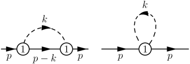
   Figure 4.5: One-loop contributions to the nucleon self-energy

3. Use the Feynman rules to show that the second diagram in Figure 4.5 does not contribute to the self energy.

4. Use the Feynman rules and the expressions for the propagators,

   $$i\Delta_{\pi}(p) = \frac{i}{p^{2}-M^{2}+i0^{+}},$$

   $$iS_{N}(p) = i\,\frac{\not{p}+\stackrel{{\scriptstyle\circ}}{{m}}_{N}-i0^{+}}{p^{2}-\stackrel{{\scriptstyle\circ}}{{m}}_{N}^{2}+i0^{+}},$$

   to verify that in dimensional regularization the first diagram in Figure 4.5 gives the contribution

   $$-i\Sigma^{\rm loop}(\not{p})=-i\frac{3\stackrel{{\scriptstyle\circ}}{{g}}_{A0}^{2}}{4F_{0}^{2}}\,i\mu^{4-n}\int\frac{d^{n}k}{(2\pi)^{n}}\frac{\not{k}(\not{p}-\stackrel{{\scriptstyle\circ}}{{m}}_{N}-\not{k})\not{k}}{[(p-k)^{2}-\stackrel{{\scriptstyle\circ}}{{m}}_{N}^{2}+i0^{+}][k^{2}-M^{2}+i0^{+}]}.$$ (4.78)

5. Show that the numerator can be simplified to

   $$-(\not{p}+\stackrel{{\scriptstyle\circ}}{{m}}_{N})k^{2}+(p^{2}-\stackrel{{\scriptstyle\circ}}{{m}}_{N}^{2})\not{k}-\left[(p-k)^{2}-\stackrel{{\scriptstyle\circ}}{{m}}_{N}^{2}\right]\not{k},$$ (4.79)

   which, when inserted in Eq. (4.78), gives

   $$\Sigma^{\rm loop}(\not{p})=\frac{3\stackrel{{\scriptstyle\circ}}{{g}}_{A0}^{2}}{4F_{0}^{2}}\,\left\{-(\not{p}+\stackrel{{\scriptstyle\circ}}{{m}}_{N})\mu^{4-n}i\int\frac{d^{n}k}{(2\pi)^{n}}\frac{1}{[(p-k)^{2}-\stackrel{{\scriptstyle\circ}}{{m}}_{N}^{2}+i0^{+}]}\right.$$ (4.80)

   $$-(\not{p}+\stackrel{{\scriptstyle\circ}}{{m}}_{N})M^{2}\mu^{4-n}i\int\frac{d^{n}k}{(2\pi)^{n}}\frac{1}{[(p-k)^{2}-\stackrel{{\scriptstyle\circ}}{{m}}_{N}^{2}+i0^{+}][k^{2}-M^{2}+i0^{+}]}$$

   $$+(p^{2}-\stackrel{{\scriptstyle\circ}}{{m}}_{N}^{2})\mu^{4-n}i\int\frac{d^{n}k}{(2\pi)^{n}}\frac{\not{k}}{[(p-k)^{2}-\stackrel{{\scriptstyle\circ}}{{m}}_{N}^{2}+i0^{+}][k^{2}-M^{2}+i0^{+}]}$$

   $$\left.-\mu^{4-n}i\int\frac{d^{n}k}{(2\pi)^{n}}\frac{\not{k}}{[k^{2}-M^{2}+i0^{+}]}\right\}.$$

   Hint: $\{\gamma_{\mu},\gamma_{\nu}\}=2g_{\mu\nu},\quad\{\gamma_{\mu},\gamma_{5}\}=0,\quad\gamma_{5}\gamma_{5}=1,\quad k^{2}=k^{2}-M^{2}+M^{2}.$

6. The last term in Eq. (4.80) vanishes since the integrand is odd in $k$. We use the following convention for scalar loop integrals

   $$I_{N\cdots\pi\cdots}(p_{1},\cdots,q_{1},\cdots)$$

   $$=\mu^{4-n}i\int\frac{d^{n}k}{(2\pi)^{n}}\frac{1}{[(k+p_{1})^{2}-\stackrel{{\scriptstyle\circ}}{{m}}_{N}^{2}+i0^{+}]\cdots[(k+q_{1})^{2}-M^{2}+i0^{+}]\cdots}\,.$$

   To determine the vector integral use the ansatz

   $$\mu^{4-n}i\int\frac{d^{n}k}{(2\pi)^{n}}\frac{k_{\mu}}{[(p-k)^{2}-\stackrel{{\scriptstyle\circ}}{{m}}_{N}^{2}+i0^{+}][k^{2}-M^{2}+i0^{+}]}=p_{\mu}\,C.$$ (4.81)

   Multiply Eq. (4.81) by $p^{\mu}$ to show that $C$ is given by

   $$C=\frac{1}{2p^{2}}\left[I_{N}-I_{\pi}+(p^{2}-\stackrel{{\scriptstyle\circ}}{{m}}_{N}^{2}+M^{2})I_{N\pi}(-p)\right].$$ (4.82)

   Using the above convention the loop contribution to the nucleon self energy reads

   $$\Sigma^{\rm loop}(\not{p}) = -\frac{3\stackrel{{\scriptstyle\circ}}{{g}}_{A0}^{2}}{4F_{0}^{2}}\,\Bigg{\{}(\not{p}+\stackrel{{\scriptstyle\circ}}{{m}}_{N})I_{N}+(\not{p}+\stackrel{{\scriptstyle\circ}}{{m}}_{N})M^{2}I_{N\pi}(-p,0)$$

   $$-(p^{2}-\stackrel{{\scriptstyle\circ}}{{m}}_{N}^{2})\frac{\not{p}}{2p^{2}}\left[I_{N}-I_{\pi}+(p^{2}-\stackrel{{\scriptstyle\circ}}{{m}}_{N}^{2}+M^{2})I_{N\pi}(-p)\right]\Bigg{\}}.$$

   The explicit expressions for the integrals are given by

   $$I_{\pi} = \frac{M^{2}}{16\pi^{2}}\left[R+\ln{\left(\frac{M^{2}}{\mu^{2}}\right)}\right],$$

   $$I_{N} = \frac{\stackrel{{\scriptstyle\circ}}{{m}}_{N}^{2}}{16\pi^{2}}\left[R+\ln{\left(\frac{\stackrel{{\scriptstyle\circ}}{{m}}_{N}^{2}}{\mu^{2}}\right)}\right],$$

   $$I_{N\pi}(p,0) = \frac{1}{16\pi^{2}}\left[R+\ln{\left(\frac{\stackrel{{\scriptstyle\circ}}{{m}}_{N}^{2}}{\mu^{2}}\right)}-1\right.$$

   $$\left.+\frac{p^{2}-\stackrel{{\scriptstyle\circ}}{{m}}_{N}^{2}-M^{2}}{p^{2}}\ln{\left(\frac{M}{\stackrel{{\scriptstyle\circ}}{{m}}_{N}}\right)}+\frac{2\stackrel{{\scriptstyle\circ}}{{m}}_{N}M}{p^{2}}F(\Omega)\right],$$

   where

   $$R = \frac{2}{n-4}-[\ln(4\pi)+{\Gamma}^{\prime}(1)+1],$$

   $$\Omega = \frac{p^{2}-\stackrel{{\scriptstyle\circ}}{{m}}_{N}^{2}-M^{2}}{2\stackrel{{\scriptstyle\circ}}{{m}}_{N}M},$$

   and

   $$F(\Omega)=\left\{\begin{array}[]{l@{\quad}l}\sqrt{\Omega^{2}-1}\ln{\left(-\Omega-\sqrt{\Omega^{2}-1}\right)},&\Omega\leq-1,\\ \sqrt{1-\Omega^{2}}\;\arccos(-\Omega),&-1\leq\Omega\leq 1,\\ \sqrt{\Omega^{2}-1}\ln{\left(\Omega+\sqrt{\Omega^{2}-1}\right)}-i\pi\sqrt{\Omega^{2}-1},&1\leq\Omega\,.\end{array}\right.$$

7. The result for the self energy contains divergences as $n\rightarrow 4$ (the terms proportional to $R$), so it has to be renormalized. For convenience, choose the renormalization parameter $\mu=\stackrel{{\scriptstyle\circ}}{{m}}_{N}$. The $\widetilde{\rm MS}$ renormalization can be performed by simply dropping the terms proportional to $R$ and by replacing all bare coupling constants ($c_{1},\stackrel{{\scriptstyle\circ}}{{g}}_{A0},F_{0}$) with the renormalized ones, now indicated by a subscript $r$. The $\widetilde{\rm MS}$ renormalized self energy contribution then reads

   $$\Sigma^{\rm loop}_{r}(\not{p}) = -\frac{3\stackrel{{\scriptstyle\circ}}{{g}}_{Ar}^{2}}{4F_{r}^{2}}\,\Bigg{\{}(\not{p}+\stackrel{{\scriptstyle\circ}}{{m}}_{N})M^{2}I_{N\pi}^{r}(-p,0)$$

   $$-(p^{2}-\stackrel{{\scriptstyle\circ}}{{m}}_{N}^{2})\frac{\not{p}}{2p^{2}}\left[(p^{2}-\stackrel{{\scriptstyle\circ}}{{m}}_{N}^{2}+M^{2})I_{N\pi}^{r}(-p)-I_{\pi}^{r}\right]\Bigg{\}},$$

   where the superscript $r$ on the integrals means that the terms proportional to $R$ have been dropped. Using the definition of the integrals, show that Eq. (7) contains a term of order ${\cal O}(p^{2})$. What does the presence of this term tell you about the applicability of the $\widetilde{\rm MS}$ scheme in baryon ChPT?

   Hint: What chiral order did the power counting assign to the diagram from which we calculated $\Sigma^{\rm loop}$?

8. We can now solve Eq. (4.76) for the nucleon mass,

   $$m_{N} = \stackrel{{\scriptstyle\circ}}{{m}}_{N}+\Sigma^{\rm contact}_{r}(m_{N})+\Sigma^{\rm loop}_{r}(m_{N})$$ (4.86)

   $$= \stackrel{{\scriptstyle\circ}}{{m}}_{N}-4c_{1r}M^{2}+\Sigma^{\rm loop}_{r}(m_{N}).$$

   We have $m_{N}-\stackrel{{\scriptstyle\circ}}{{m}}_{N}={\cal O}(p^{2})$. Since our calculation is only valid up to order ${\cal O}(p^{3})$, determine $\Sigma^{\rm loop}_{r}(m_{N})$ to that order. Check that you only need an expansion of $I_{N\pi}^{r}$, which, using

   $$\arccos{(-\Omega)}=\frac{\pi}{2}+\cdots,$$

   verify to be

   $$I_{N\pi}^{r}=\frac{1}{16\pi^{2}}\left(-1+\frac{\pi M}{\stackrel{{\scriptstyle\circ}}{{m}}_{N}}\cdots\right).$$ (4.87)

   Show that this yields

   $$m_{N}=\stackrel{{\scriptstyle\circ}}{{m}}_{N}-4c_{1r}M^{2}+\frac{3\stackrel{{\scriptstyle\circ}}{{g}}_{Ar}^{2}M^{2}}{32\pi^{2}F_{r}^{2}}\stackrel{{\scriptstyle\circ}}{{m}}_{N}-\frac{3\stackrel{{\scriptstyle\circ}}{{g}}_{Ar}^{2}M^{3}}{32\pi^{2}F_{r}^{2}}.$$ (4.88)

9. The solution to the power counting problem is the observation that the term violating the power counting (the third on the right of Eq. (4.88)) is analytic in small quantities and can thus be absorbed in counter terms. In addition to the $\widetilde{\rm MS}$ scheme we have to perform an additional finite renormalization. Rewrite

   $$c_{1r}=c_{1}+\delta c_{1}$$ (4.89)

   in Eq. (4.88) and determine $\delta c_{1}$ so that the term violating the power counting is absorbed, which then gives the final result for the nucleon mass at order ${\cal O}(p^{3})$

   $$m_{N}=\stackrel{{\scriptstyle\circ}}{{m}}_{N}-4c_{1}M^{2}-\frac{3\stackrel{{\scriptstyle\circ}}{{g}}_{Ar}^{2}M^{3}}{32\pi^{2}F_{r}^{2}}.$$ (4.90)

We saw in Exercise 4.6.1 that, for the case of the nucleon self energy, the expression for loop diagrams renormalized by applying dimensional regularization in combination with the $\widetilde{\rm MS}$ scheme as in the mesonic sector contained terms not consistent with the power counting. The appearance of terms violating the power counting when using the $\widetilde{\rm MS}$ scheme is a general feature of loop calculations in baryonic chiral perturbation theory [Gasser:1987rb:5]. However, in the example above these terms were analytic in small parameters and could be absorbed by an additional finite renormalization. The question arises if this can be done in general. Indeed, there are several renormalization schemes that yield a consistent power counting for the baryonic sector of chiral perturbation theory. They make use of the observation that the terms violating the power counting are analytic in small parameters and can thus be absorbed in the available parameters. We briefly mention two methods without going into any details.

In the infrared regularization of Becher and Leutwyler [Becher:1999he:5], one-loop integrals are split into two pieces,

$$H=\int_{0}^{1}dx\cdots = \int_{0}^{\infty}dx\cdots-\int_{1}^{\infty}dx\cdots$$

$$= I+R,$$

where $I$ satisfies the power counting, whereas $R$ violates it and is absorbed in counterterms.

In the extended-on-mass-shell (EOMS) scheme [Fuchs:2003qc:5], the integrand of loop integrals is expanded in small parameters, and the (integrated) terms violating the power counting are then subtracted. The advantage of the EOMS scheme is that it can also be applied in the case of diagrams containing resonances [Fuchs:2003sh:5] as well as multi-loop diagrams [Schindler:2003je:5].

Applying similar techniques as in Exercise 4.6.1, the result for the mass of the nucleon at ${\cal O}(p^{4})$ in the EOMS scheme is given by [Fuchs:2003qc:5, Fuchs:2003kq:5:1]

$$m_{N}=\stackrel{{\scriptstyle\circ}}{{m}}_{N}+k_{1}M^{2}+k_{2}M^{3}+k_{3}M^{4}\ln\left(\frac{M}{\stackrel{{\scriptstyle\circ}}{{m}}_{N}}\right)+k_{4}M^{4}+{\cal O}(M^{5}),$$ (4.91)

where the coefficients $k_{i}$ are given by

$$k_{1}=-4c_{1},\quad k_{2}=-\frac{3{\stackrel{{\scriptstyle\circ}}{{g_{A}}}}^{2}}{32\pi F^{2}},\quad k_{3}=\frac{3}{32\pi^{2}F^{2}}\left(8c_{1}-c_{2}-4c_{3}-\frac{{\stackrel{{\scriptstyle\circ}}{{g_{A}}}}^{2}}{\stackrel{{\scriptstyle\circ}}{{m}}_{N}}\right),$$

$$k_{4}=\frac{3{\stackrel{{\scriptstyle\circ}}{{g_{A}}}}^{2}}{32\pi^{2}F^{2}\stackrel{{\scriptstyle\circ}}{{m}}_{N}}(1+4c_{1}\stackrel{{\scriptstyle\circ}}{{m}}_{N})+\frac{3}{128\pi^{2}F^{2}}c_{2}+\frac{1}{2}\alpha.$$ (4.92)

Here, $\alpha=-4(8e_{38}+e_{115}+e_{116})$ is a linear combination of ${\cal O}(p^{4})$ coefficients. In order to obtain an estimate for the various contributions of Eq. (4.91) to the nucleon mass, we make use of the set of parameters $c_{i}$ of Eq. (4.71). Using the numerical values

$$g_{A}=1.267,\quad F_{\pi}=92.4\,\mbox{MeV},\quad m_{N}=938.3\,\mbox{MeV},\quad M_{\pi}=139.6\,\mbox{MeV},$$

we obtain for the mass of nucleon in the chiral limit (at fixed $m_{s}\neq 0$):

$$\stackrel{{\scriptstyle\circ}}{{m}}_{N}=m_{N}-\Delta m=[938.3-74.8+15.3+4.7+1.6-2.3]\,\mbox{MeV}=882.8\,\mbox{MeV}$$

with $\Delta m=55.5\,\mbox{MeV}$. Here, we have made use of an estimate for $\alpha$ obtained from the $\sigma$ term (see Ref. [Fuchs:2003kq:5:1] for more details). The chiral expansion reveals a good convergence and it will be interesting to further study the convergence at the two-loop level.

	Chiral limit: $M_{0}$	$M_{(2)}$	$M_{(3)}$	Sum at ${\cal O}(p^{3})$: $M_{3}$
$M_{N}$	1039	240	$-339$	940
$M_{\Sigma}$	1039	849	$-696$	1192
$M_{\Lambda}$	1039	811	$-737$	1113
$M_{\Xi}$	1039	1400	$-1120$	1319
$\sigma_{\pi N}$	—	85	$-40$	45

Table 4.3: Baryon masses in MeV and their individual contributions. Note that the free parameters have been fit so that the masses at ${\cal O}(p^{3})$ essentially agree with the physical masses.

Finally, it is straightforward but more tedious to apply the same techniques to an SU(3) calculation of the masses of the baryon octet [Lehnhart:2004vi:5:1]. The results and their individual contributions are shown in Table 4.3. Large cancellations between the contributions $M_{(2)}$ and $M_{(3)}$ at ${\cal O}(p^{2})$ and ${\cal O}(p^{3})$, respectively, are a well-known feature. In Figure 4.6 we show how “switching on” the quark masses affects the masses of the baryon octet. In the chiral limit all masses reduce to $M_{0}=1039$ MeV. Keeping the up and down quarks massless, we still have an $\mbox{SU(2)}_{L}\times\mbox{SU(2)}_{R}$ symmetry resulting in

$$M_{\pi,2}^{2}=0,~{}~{}~{}M_{K,2}^{2}~{}=~{}B_{0}m_{s},~{}~{}~{}M_{\eta,2}^{2}~{}=~{}\frac{4}{3}B_{0}m_{s}~{}=~{}\frac{4}{3}M_{K,2}^{2}.$$ (4.93)

The corresponding values of the mass spectrum are shown in the middle panel of Figure 4.6 ($M_{\pi}=0$, $M_{K}=486$ MeV and $M_{\eta}=562$ MeV), while the final results, exhibiting only an $\mbox{SU(2)}_{V}$ symmetry, are shown in the right panel.

Figure 4.6: Mass level diagram depending on the various symmetries. Left panel: $\mbox{SU(3)}_{L}\times\mbox{SU(3)}_{R}$ symmetry; middle panel: $\mbox{SU(2)}_{L}\times\mbox{SU(2)}_{R}$ symmetry; right panel: $\mbox{SU(2)}_{V}$ symmetry.

4.6.2 The Generation of Counterterms *

The renormalization of the effective field theory (of pions and nucleons) is performed by expressing all the bare parameters and bare fields of the effective Lagrangian in terms of renormalized quantities (see Ref. [Collins:xc:5:2] for details). In this process, one generates counterterms which are responsible for the absorption of all the divergences occurring in the calculation of loop diagrams. In order to illustrate the procedure let us discuss ${\cal L}_{\pi N}^{(1)}$ and consider the free part in combination with the $\pi N$ interaction term with the smallest number of pion fields,

$${\cal L}_{\pi N}^{(1)}=\bar{\Psi}_{0}\left(i\gamma_{\mu}\partial^{\mu}-m_{0}-\frac{1}{2}\frac{{\stackrel{{\scriptstyle\circ}}{{g}}_{A}}_{0}}{F_{0}}\gamma_{\mu}\gamma_{5}\tau^{a}\partial^{\mu}\pi^{a}_{0}\right)\Psi_{0}+\cdots,$$ (4.94)

given in terms of bare fields and parameters denoted by subscripts 0. Introducing renormalized fields (we work in the isospin-symmetric limit) through

$$\Psi=\frac{\Psi_{0}}{\sqrt{Z_{\Psi}}},\quad\pi^{a}=\frac{\pi^{a}_{0}}{\sqrt{Z_{\pi}}},$$ (4.95)

we express the field redefinition constants $\sqrt{Z_{\Psi}}$ and $\sqrt{Z_{\pi}}$ and the bare quantities in terms of renormalized parameters:

$$Z_{\Psi} = 1+\delta Z_{\Psi}\left(\stackrel{{\scriptstyle\circ}}{{m}}_{N},\stackrel{{\scriptstyle\circ}}{{g}}_{A},g_{i},\nu\right),$$

$$Z_{\pi} = 1+\delta Z_{\pi}\left(\stackrel{{\scriptstyle\circ}}{{m}}_{N},\stackrel{{\scriptstyle\circ}}{{g}}_{A},g_{i},\nu\right),$$

$$m_{0} = \stackrel{{\scriptstyle\circ}}{{m}}_{N}(\nu)+\delta m\left(\stackrel{{\scriptstyle\circ}}{{m}}_{N},\stackrel{{\scriptstyle\circ}}{{g}}_{A},g_{i},\nu\right),$$

$${\stackrel{{\scriptstyle\circ}}{{g}}_{A}}_{0} = \stackrel{{\scriptstyle\circ}}{{g}}_{A}(\nu)+\delta g_{A}\left(\stackrel{{\scriptstyle\circ}}{{m}}_{N},\stackrel{{\scriptstyle\circ}}{{g}}_{A},g_{i},\nu\right),$$ (4.96)

where $g_{i}$, $i=1,\cdots,\infty$, collectively denote all the renormalized parameters which correspond to bare parameters ${g_{i}}_{0}$ of the full effective Lagrangian. The parameter $\nu$ indicates the dependence on the choice of the renormalization prescription. Substituting Eqs. (4.95) and (4.96) into Eq. (4.94), we obtain

$${\cal L}_{\pi N}^{(1)}={\cal L}_{\rm basic}+{\cal L}_{\rm ct}+\cdots$$ (4.97)

with the so-called basic and counterterm Lagrangians, respectively,

$${\cal L}_{\rm basic} = \bar{\Psi}\left(i\gamma_{\mu}\partial^{\mu}-\stackrel{{\scriptstyle\circ}}{{m}}_{N}-\frac{1}{2}\frac{\stackrel{{\scriptstyle\circ}}{{g}}_{A}}{F}\gamma_{\mu}\gamma_{5}\tau^{a}\partial^{\mu}\pi^{a}\right)\Psi,$$ (4.98)

$${\cal L}_{\rm ct} = \delta Z_{\Psi}\bar{\Psi}i\gamma_{\mu}\partial^{\mu}\Psi-\delta\{m\}\bar{\Psi}\Psi-\frac{1}{2}\delta\left\{\frac{\stackrel{{\scriptstyle\circ}}{{g}}_{A}}{F}\right\}\bar{\Psi}\gamma_{\mu}\gamma_{5}\tau^{a}\partial^{\mu}\pi^{a}\Psi,$$

where we introduced the abbreviations

$$\delta\{m\} \equiv \delta Z_{\Psi}m+Z_{\Psi}\delta m,$$

$$\delta\left\{\frac{\stackrel{{\scriptstyle\circ}}{{g}}_{A}}{F}\right\} \equiv \delta Z_{\Psi}\frac{\stackrel{{\scriptstyle\circ}}{{g}}_{A}}{F}\sqrt{Z_{\pi}}+Z_{\Psi}\left(\frac{{\stackrel{{\scriptstyle\circ}}{{g}}_{A}}_{0}}{F_{0}}-\frac{\stackrel{{\scriptstyle\circ}}{{g}}_{A}}{F}\right)\sqrt{Z_{\pi}}+\frac{\stackrel{{\scriptstyle\circ}}{{g}}_{A}}{F}(\sqrt{Z_{\pi}}-1).$$

In Eq. (4.98), $\stackrel{{\scriptstyle\circ}}{{m}}_{N}$, $\stackrel{{\scriptstyle\circ}}{{g}}_{A}$, and $F$ denote the chiral limit of the physical nucleon mass, the axial-vector coupling constant, and the pion-decay constant, respectively. Expanding the counterterm Lagrangian of Eq. (4.6.2) in powers of the renormalized coupling constants generates an infinite series, the individual terms of which are responsible for the subtraction of loop diagrams.

References:

- [1] H. Leutwyler, in Perspectives in the Standard Model, Proceedings of the 1991 Advanced Theoretical Study Institute in Elementary Particle Physics, Boulder, Colorado, 2 - 28 June, 1991, edited by R. K. Ellis, C. T. Hill, and J. D. Lykken (World Scientific, Singapore, 1992)
- [2] J. Bijnens, Int. J. Mod. Phys. A 8, 3045 (1993)
- [3] U.-G. Meißner, Rept. Prog. Phys. 56, 903 (1993)
- [4] H. Leutwyler, in Hadron Physics 94: Topics on the Structure and Interaction of Hadronic Systems, Proceedings, Workshop, Gramado, Brasil, edited by V. E. Herscovitz (World Scientific, Singapore, 1995)
- [5] V. Bernard, N. Kaiser, and U.-G. Meißner, Int. J. Mod. Phys. E 4, 193 (1995)
- [6] E. de Rafael, in CP Violation and the Limits of the Standard Model, Proceedings of the 1994 Advanced Theoretical Study Institute in Elementary Particle Physics, Boulder, Colorado, 29 May - 24 June, 1994, edited by J. F. Donoghue (World Scientific, Singapore, 1995).
- [7] A. Pich, Rept. Prog. Phys. 58, 563 (1995)
- [8] G. Ecker, Prog. Part. Nucl. Phys. 35, 1 (1995)
- [9] A. V. Manohar, Lectures given at 35th Int. Universitätswochen für Kern- und Teilchenphysik: Perturbative and Nonperturbative Aspects of Quantum Field Theory, Schladming, Austria, 2 - 9 March, 1996, arXiv:hep-ph/9606222
- [10] A. Pich, in Probing the Standard Model of Particle Interactions, Proceedings of the Les Houches Summer School in Theoretical Physics, Session 68, Les Houches, France, 28 July - 5 September 1997, edited by R. Gupta, A. Morel, E. de Rafael, and F. David (Elsevier, Amsterdam, 1999)
- [11] C. P. Burgess, Phys. Rept. 330, 193 (2000)
- [12] S. Scherer, in Advances in Nuclear Physics, Vol. 27, edited by J. W. Negele and E. W. Vogt (Kluwer Academic/Plenum Publishers, New York, 2003)
- [13] A. M. Bernstein and B. R. Holstein (Eds.), Chiral Dynamics: Theory and Experiment. Proceedings, Workshop, Cambridge, USA, 25 - 29 July, 1994 (Springer, Berlin, 1995, Lecture Notes in Physics, Vol. 452)
- [14] A. M. Bernstein, D. Drechsel, and Th. Walcher (Eds.), Chiral Dynamics: Theory and Experiment. Proceedings, Workshop, Mainz, Germany, 1 - 5 September, 1997, (Springer, Berlin, 1998, Lecture Notes in Physics, Vol. 513)
- [15] A. M. Bernstein, J. L. Goity, and U.-G. Meißner (Eds.), Chiral Dynamics: Theory and Experiment III. Proceedings, Workshop, Jefferson Laboratory, USA, 17 - 20 July, 2000 (World Scientific, Singapore, 2002)
- [16] U.-G. Meißner, H. W. Hammer, and A. Wirzba, arXiv:hep-ph/0311212

References:

- [1] A. P. Balachandran and C. G. Trahern, Lectures On Group Theory For Physicists (Bibliopolis, Naples, 1984)
- [2] H. F. Jones, Groups, Representations and Physics (Hilger, Bristol, 1990)
- [3] L. O’Raifeartaigh, Group Structure of Gauge Theories (Cambridge University Press, Cambridge, 1986)
-
[4]
S. Scherer, Gruppentheorie in der Physik I + II
(http://kph.uni-mainz.de/T/lecture.html) - [5] V. I. Borodulin, R. N. Rogalev, and S. R. Slabospitsky, arXiv:hep-ph/9507456

References:

- [1] D. J. Gross and F. Wilczek, Phys. Rev. Lett. 30, 1343 (1973)
- [2] S. Weinberg, Phys. Rev. Lett. 31, 494 (1973)
- [3] H. Fritzsch, M. Gell-Mann, and H. Leutwyler, Phys. Lett. B 47, 365 (1973)
- [4] W. J. Marciano and H. Pagels, Phys. Rept. 36, 137 (1978)
- [5] G. Altarelli, Phys. Rept. 81, 1 (1982)
- [6] T.-P. Cheng and L.-F. Li, Gauge theory of elementary particle physics (Clarendon, Oxford, 1984), Chapter 10
- [7] J. F. Donoghue, E. Golowich, and B. R. Holstein, Dynamics of the Standard Model (Cambridge University Press, Cambridge, 1992) Chapter II-2
- [8] F. Scheck, Electroweak and Strong Interactions: An Introduction to Theoretical Particle Physics (Springer, Berlin, 1996), Chapter 3.5
- [9] A. Manohar, Quark Masses, in D. E. Groom et al. [Particle Data Group Collaboration], Eur. Phys. J. C 15, 1 (2000)

References:

- [1] E. L. Hill, Rev. Mod. Phys. 23, 253 (1951)
- [2] M. Gell-Mann and M. Lévy, Nuovo Cim. 16, 705 (1960)
- [3] V. de Alfaro, S. Fubini, G. Furlan, and C. Rossetti, Currents in Hadron Physics (North-Holland, Amsterdam, 1973), Chapter 2.1.1
- [4] Any book on quantum field theory

References:

- [1] M. Gell-Mann, Phys. Rev. 125, 1067 (1962)

References:

- [1] S. L. Glashow and S. Weinberg, Phys. Rev. Lett. 20, 224 (1968)
- [2] M. Gell-Mann, R. J. Oakes, and B. Renner, Phys. Rev. 175, 2195 (1968)
- [3] M. Gell-Mann and Y. Ne’eman, The Eightfold Way (Benjamin, New York, 1964)
- [4] M. Gell-Mann, Physics 1, 63 (1964)
- [5] S. L. Adler and R. F. Dashen, Current Algebras and Applications to Particle Physics (Benjamin, New York, 1968)

References:

- [1] J. Zinn-Justin, Quantum Field Theory And Critical Phenomena (Clarendon, Oxford, 1989)
- [2] A. Das, Field Theory: A Path Integral Approach (World Scientific, Singapore, 1993)

References:

- [1] J. S. Schwinger, Phys. Rev. Lett. 3, 296 (1959)
- [2] R. Jackiw, Field Theoretic Investigations in Current Algebra, in S. Treiman, R. Jackiw, and D. J. Gross, Lectures on Current Algebra and Its Applications (Princeton University Press, Princeton, 1972)

References:

- [1] H. Leutwyler, Annals Phys. 235, 165 (1994)
- [2] J. Gasser and H. Leutwyler, Annals Phys. 158, 142 (1984)
- [3] J. Gasser and H. Leutwyler, Nucl. Phys. B250, 465 (1985)

References:

- [1] S. L. Adler, Phys. Rev. 139, B1638 (1965)

References:

- [1] Y. Nambu, Phys. Rev. Lett. 4, 380 (1960)
- [2] Y. Nambu and G. Jona-Lasinio, Phys. Rev. 122, 345 (1961); Phys. Rev. 124, 246 (1961)
- [3] J. Goldstone, Nuovo Cim. 19, 154 (1961)
- [4] J. Goldstone, A. Salam, and S. Weinberg, Phys. Rev. 127, 965 (1962)
- [5] L. F. Li and H. Pagels, Phys. Rev. Lett. 26, 1204 (1971)
- [6] J. Bernstein, Rev. Mod. Phys. 46, 7 (1974) [Erratum, ibid. 47, 259 (1975)]
- [7] L. H. Ryder, Quantum Field Theory (Cambridge University Press, Cambridge, 1985) Chapter 8
- [8] T. P. Cheng and L. F. Li, Gauge Theory of Elementary Particle Physics (Clarendon, Oxford, 1984) Chapter 5.3
- [9] H. Georgi, Weak Interactions and Modern Particle Theory (Benjamin/Cummings, Menlo Park, 1984) Chapter 2.4 - 2.6
- [10] S. Weinberg, The Quantum Theory Of Fields. Vol. 2: Modern Applications (Cambridge University Press, Cambridge, 1996) Chapter 19

References:

- [1] J. Polchinski, arXiv:hep-th/9210046
- [2] H. Georgi, Ann. Rev. Nucl. Part. Sci. 43, 207 (1993)
- [3] D. B. Kaplan, arXiv:nucl-th/9506035
- [4] A. V. Manohar, arXiv:hep-ph/9606222
- [5] A. Pich, arXiv:hep-ph/9806303

References:

- [1] Y. Nambu, Phys. Rev. Lett. 4, 380 (1960)
- [2] Y. Nambu and G. Jona-Lasinio, Phys. Rev. 122, 345 (1961); Phys. Rev. 124, 246 (1961)
- [3] J. Goldstone, Nuovo Cim. 19, 154 (1961)
- [4] J. Goldstone, A. Salam, and S. Weinberg, Phys. Rev. 127, 965 (1962)
- [5] S. Coleman, J. Math. Phys. 7, 787 (1966)
- [6] C. Vafa and E. Witten, Nucl. Phys. B234, 173 (1984)
- [7] T. P. Cheng and L. F. Li, Gauge Theory of Elementary Particle Physics (Clarendon, Oxford, 1984) Chapter 5.3

References:

- [1] G. Colangelo, J. Gasser, and H. Leutwyler, Phys. Rev. Lett. 86, 5008 (2001)

References:

- [1] S. Weinberg, Phys. Rev. 166, 1568 (1968)
- [2] S. R. Coleman, J. Wess, and B. Zumino, Phys. Rev. 177, 2239 (1969)
- [3] C. G. Callan, S. R. Coleman, J. Wess, and B. Zumino, Phys. Rev. 177, 2247 (1969)
- [4] A. P. Balachandran, G. Marmo, B. S. Skagerstam, and A. Stern, Classical Topology and Quantum States (World Scientific, Singapore, 1991) Chapter 12.2
- [5] H. Leutwyler, in Perspectives in the Standard Model, Proceedings of the 1991 Advanced Theoretical Study Institute in Elementary Particle Physics, Boulder, Colorado, 2 - 28 June, 1991, edited by R. K. Ellis, C. T. Hill, and J. D. Lykken (World Scientific, Singapore, 1992)

References:

- [1] J. Gasser and H. Leutwyler, Annals Phys. 158, 142 (1984)
- [2] J. Gasser and H. Leutwyler, Nucl. Phys. B250, 465 (1985)
- [3] H. Georgi, Weak Interactions and Modern Particle Theory (Benjamin/Cummings, Menlo Park, 1984)
- [4] M. Gell-Mann, R. J. Oakes, and B. Renner, Phys. Rev. 175, 2195 (1968)
- [5] M. Knecht, B. Moussallam, J. Stern, and N. H. Fuchs, Nucl. Phys. B457, 513 (1995)
- [6] S. Pislak et al. [BNL-E865 Collaboration], Phys. Rev. Lett. 87, 221801 (2001)
- [7] G. Colangelo, J. Gasser, and H. Leutwyler, Phys. Rev. Lett. 86, 5008 (2001)

References:

- [1] S. Weinberg, Physica A 96, 327 (1979)
- [2] C. Itzykson and J. B. Zuber, Quantum Field Theory (McGraw-Hill, New York, 1980), Appendix A-4
- [3] H. Leutwyler, Annals Phys. 235, 165 (1994)
- [4] E. D’Hoker and S. Weinberg, Phys. Rev. D 50, 6050 (1994)

References:

- [1] H. W. Fearing and S. Scherer, Phys. Rev. D 53, 315 (1996)
- [2] J. Bijnens, G. Colangelo, and G. Ecker, JHEP 9902, 020 (1999)
- [3] T. Ebertshäuser, Mesonic Chiral Perturbation Theory: Odd Intrinsic Parity Sector, PhD thesis, Johannes Gutenberg-Universität, Mainz, Germany, 2001, http://archimed.uni-mainz.de/
- [4] T. Ebertshäuser, H. W. Fearing, and S. Scherer, Phys. Rev. D 65, 054033 (2002)
- [5] J. Bijnens, L. Girlanda, and P. Talavera, Eur. Phys. J. C 23, 539 (2002)

References:

- [1] J. Gasser and H. Leutwyler, Nucl. Phys. B250, 465 (1985)

References:

- [1] S. Weinberg, Phys. Rev. Lett. 17, 616 (1966)
- [2] J. Gasser and H. Leutwyler, Annals Phys. 158, 142 (1984)
- [3] M. A. Preston, Physics of the Nucleus (Addison-Wesley, Reading, MA, 1962)
- [4] J. Bijnens, G. Colangelo, G. Ecker, J. Gasser, and M. E. Sainio, Phys. Lett. B 374, 210 (1996)
- [5] G. Colangelo, J. Gasser, and H. Leutwyler, Phys. Rev. Lett. 86, 5008 (2001)
- [6] G. Colangelo, J. Gasser, and H. Leutwyler, Nucl. Phys. B603, 125 (2001)

References:

- [1] J. Bijnens and F. Cornet, Nucl. Phys. B296, 557 (1988)
- [2] C. Unkmeir, S. Scherer, A. I. L’vov, and D. Drechsel, Phys. Rev. D 61, 034002 (2000)

References:

- [1] J. Gasser and H. Leutwyler, Nucl. Phys. B250, 465 (1985)
- [2] S. Weinberg, The Quantum Theory of Fields. Vol. 1: Foundations (Cambridge University Press, Cambridge, 1995), Chapter 12
- [3] J. Bijnens, G. Ecker, and J. Gasser, in The Second DANE Physics Handbook, edited by L. Maiani, G. Pancheri, and N. Paver (Frascati, Italy, 1995)

References:

- [1] G. ’t Hooft and M. J. Veltman, Nucl. Phys. B44, 189 (1972)
- [2] G. Leibbrandt, Rev. Mod. Phys. 47, 849 (1975)
- [3] G. ’t Hooft and M. J. Veltman, Nucl. Phys. B153, 365 (1979)
- [4] T. P. Cheng and L. F. Li, Gauge Theory of Elementary Particle Physics (Clarendon, Oxford, 1984), Chapter 2
- [5] J. C. Collins, Renormalization (Cambridge University Press, Cambridge, 1984)
- [6] M. J. Veltman, Diagrammatica. The Path to Feynman Rules (Cambridge University Press, Cambridge, 1994)
- [7] Any modern book on quantum field theory.

References:

- [1] J. Gasser and H. Leutwyler, Annals Phys. 158, 142 (1984)
- [2] J. Gasser and H. Leutwyler, Nucl. Phys. B250, 465 (1985)
- [3] J. Gasser, M. E. Sainio, and A. Švarc, Nucl. Phys. B307, 779 (1988)
- [4] L. F. Li and H. Pagels, Phys. Rev. Lett. 26, 1204 (1971)
- [5] T. P. Cheng and L. F. Li, Gauge Theory of Elementary Particle Physics (Clarendon, Oxford, 1984) Chapter 2

References:

- [1] S. Weinberg, Phys. Rev. 166, 1568 (1968)
- [2] S. R. Coleman, J. Wess, and B. Zumino, Phys. Rev. 177, 2239 (1969)
- [3] C. G. Callan, S. R. Coleman, J. Wess, and B. Zumino, Phys. Rev. 177, 2247 (1969)
- [4] H. Georgi, Weak Interactions and Modern Particle Theory (Benjamin/Cummings, Menlo Park, 1984)
- [5] J. Gasser, M. E. Sainio, and A. Švarc, Nucl. Phys. B307, 779 (1988)

References:

- [1] J. Gasser, M. E. Sainio, and A. Švarc, Nucl. Phys. B307, 779 (1988)
- [2] L. L. Foldy and S. A. Wouthuysen, Phys. Rev. 78, 29 (1950)
- [3] H. W. Fearing, G. I. Poulis, and S. Scherer, Nucl. Phys. A570, 657 (1994)
- [4] A. Krause, Helv. Phys. Acta 63, 3 (1990)
- [5] E. Jenkins and A. V. Manohar, Phys. Lett. B 255, 558 (1991)
- [6] V. Bernard, N. Kaiser, J. Kambor, and U.-G. Meißner, Nucl. Phys. B388, 315 (1992)
- [7] H. Georgi, Weak Interactions and Modern Particle Theory (Benjamin/Cummings, Menlo Park, 1984)
- [8] B. Borasoy, Phys. Rev. D 59, 054021 (1999)

References:

- [1] M. L. Goldberger and S. B. Treiman, Phys. Rev. 110, 1178 (1958); Phys. Rev. 111, 354 (1958)
- [2] Y. Nambu, Phys. Rev. Lett. 4, 380 (1960)
- [3] S. Weinberg, Phys. Rev. 112, 1375 (1958)
- [4] H. C. Schröder et al., Eur. Phys. J. C 21, 473 (2001)
- [5] T. Fuchs and S. Scherer, Phys. Rev. C 68, 055501 (2003)

References:

- [1] S. Weinberg, Phys. Rev. Lett. 17, 616 (1966)
- [2] Y. Tomozawa, Nuovo Cim. 46 A, 707 (1966)
- [3] M. Mojžiš, Eur. Phys. J. C 2, 181 (1998)
- [4] N. Fettes and U.-G. Meißner, Nucl. Phys. A676, 311 (2000)
- [5] T. Becher and H. Leutwyler, JHEP 0106, 017 (2001)
- [6] R. Koch, Nucl. Phys. A448, 707 (1986)
- [7] E. Matsinos, Phys. Rev. C 56, 3014 (1997)
- [8] H. C. Schröder et al., Eur. Phys. J. C 21, 473 (2001)

References:

- [1] J. Gasser, M. E. Sainio, and A. Švarc, Nucl. Phys. B307, 779 (1988)
- [2] N. Fettes, U.-G. Meißner, M. Mojžiš, and S. Steininger, Annals Phys. 283, 273 (2001) [Erratum, ibid. 288, 249 (2001)]
- [3] T. Becher and H. Leutwyler, JHEP 0106, 017 (2001)
- [4] R. Koch, Nucl. Phys. A448, 707 (1986)

References:

- [1] J. Gasser, M. E. Sainio, and A. Švarc, Nucl. Phys. B307, 779 (1988)
- [2] T. Becher and H. Leutwyler, Eur. Phys. J. C 9, 643 (1999)
- [3] T. Fuchs, J. Gegelia, G. Japaridze, and S. Scherer, Phys. Rev. D 68, 056005 (2003)
- [4] T. Fuchs, M. R. Schindler, J. Gegelia, and S. Scherer, Phys. Lett. B 575, 11 (2003)
- [5] M. R. Schindler, J. Gegelia, and S. Scherer, Nucl. Phys. B682, 367 (2004)
- [6] T. Fuchs, J. Gegelia, and S. Scherer, Eur. Phys. J. A 19, 35 (2004)
- [7] B. C. Lehnhart, J. Gegelia, and S. Scherer, J. Phys. G 31, 89 (2005)

References:

- [1] J. C. Collins, Renormalization (Cambridge University Press, Cambridge, 1984)