Non-linear screening effects
in high energy hadronic interactions

Abstract

Non-linear effects in hadronic interactions are treated by means of enhanced pomeron diagrams, assuming that pomeron-pomeron coupling is dominated by soft partonic processes. It is shown that the approach allows to resolve a seeming contradiction between realistic parton momentum distributions, measured in deep inelastic scattering experiments, and the energy behavior of total proton-proton cross section. Also a general consistency with both “soft” and “hard” diffraction data is demonstrated. An important feature of the proposed scheme is that the contribution of semi-hard processes to the interaction eikonal contains a significant non-factorizable part. On the other hand, the approach preserves the QCD factorization picture for inclusive high-$p_{t}$ jet production.

1 Introduction

One of the most important issues in high energy physics is the interplay between soft and hard processes in hadronic interactions. The latter involve parton evolution in the region of comparatively high virtualities $q^{2}$ and can be treated within the perturbative QCD framework. Despite the smallness of the running coupling $\alpha_{{\rm s}}(q^{2})$ involved, corresponding contributions are expected to dominate hadronic interactions at sufficiently high energies, being enhanced by large parton multiplicities and by large logarithmic ratios of parton transverse and longitudinal momenta [1]. On the other hand, very peripheral hadronic collisions are likely to remain governed by non-perturbative soft partonic processes, whose contribution to elastic scattering amplitude thus remains significant even at very high energies. Furthermore, considering production of high transverse momentum particles, one may expect that a significant part of the underlying parton cascades, which mediate the interaction, develops in the non-perturbative low virtuality region [2], apart from the fact that additional soft re-scattering processes may proceed in parallel to the mentioned “semi-hard” ones.

A popular scheme for a combined description of soft and hard processes is the mini-jet approach [3], employed in a number of Monte Carlo generators [4]. There, one treats hadronic collisions within the eikonal framework, considering the interaction eikonal to be the sum of “soft” and “semi-hard” contributions:

$$\chi_{ad}(s,b)=\frac{1}{2}\sigma_{ad}^{{\rm soft}}(s)\>A_{ad}(b)+\frac{1}{2}\sigma_{ad}^{{\rm mini-jet}}(s,p_{t,{\rm min}})\>A_{ad}(b)\,,$$ (1)

where the overlap function $A_{ad}(b)$ is the convolution of electro-magnetic form-factors of hadrons $a$ and $d$, $A_{ad}(b)=\int\!d^{2}b^{\prime}\;T_{a}^{{\rm e/m}}(b^{\prime})\;T_{d}^{{\rm e/m}}(|\vec{b}-\vec{b}^{\prime}|)$, $\sigma_{ad}^{{\rm soft}}(s)$ - a parameterized “soft” parton cross section, and $\sigma_{ad}^{{\rm mini-jet}}(s,p_{t,{\rm min}})$ is the inclusive cross section for production of parton jets with transverse momentum bigger than a chosen cutoff $p_{t,{\rm min}}$, for which the leading logarithmic QCD result is generally used.

Qualitatively similar is the “semi-hard pomeron” scheme [5, 6], where hadronic interactions are treated within the Gribov’s reggeon approach [7, 8] as multiple exchanges of “soft” and “semi-hard” pomerons, the two objects corresponding to soft and semi-hard re-scattering processes.

However, both approaches face a fundamental difficulty when confronted with available experimental data: it appears impossible to accommodate realistic parton momentum distributions, when calculating the mini-jet cross section $\sigma_{ad}^{{\rm mini-jet}}$ in (1), without being in contradiction with moderately slow energy rise of total proton-proton cross section. It seems natural to relate this problem to the contribution of non-linear parton processes, which are missing in the above-discussed eikonal scheme. Indeed, the need for such corrections appears quite evident when considering small $x$ behavior of parton momentum distribution functions (PDFs) at some finite virtuality scale $Q^{2}$: due to a fast increase of, e.g., gluon PDF $G(x,Q^{2})$ in the $x\rightarrow 0$ limit parton density in a restricted volume may reach arbitrarily large values [1]. In the QCD framework one describes non-linear parton effects as merging of parton ladders, some typical contributions shown in Fig. 1.

Figure 1: Examples of diagrams giving rise to non-linear parton effects; increasing parton virtualities are indicated as narrowing of the ladders.

In particular, one may account for such corrections in the perturbative evolution of parton distributions, which leads to the saturation of parton densities [1, 9]. Moving towards smaller and smaller parton momentum fractions $x$, one obtains a higher saturation scale $Q_{{\rm sat}}^{2}(x)$, with a dynamical parton evolution being only possible in the region of sufficiently high virtualities $|q|^{2}>Q_{{\rm sat}}^{2}(x)$.

Using the mini-jet approach, one usually suggests some energy dependence for the transverse momentum cutoff $p_{t,{\rm min}}$ for mini-jet production, i.e. $p_{t,{\rm min}}=p_{t,{\rm min}}(s)$, and proceeds further with the usual eikonal expression (1). There, the $p_{t}$-cutoff plays the role of an effective “saturation scale”, for which a variety of empirical parameterizations has been proposed [10]. The underlying idea is to take effectively into account the contributions of diagrams of Fig. 1(left), where non-linear corrections (merging ladders) can be absorbed into parton distributions. Unfortunately, introducing such empirical parameterizations for the $p_{t}$-cutoff, one loses the connection to the perturbative QCD and spoils predictive power of the method; the “saturation scale” is chosen irrespective the actual parton densities, which depend on the parton momenta, on the “centrality” of the interaction, and on the projectile and target mass numbers in case of nuclear collisions. On the other hand, there is no good reason for keeping the simple relation (1) between the interaction eikonal and the mini-jet cross section, when contributions of graphs of Fig. 1(right) are taken into account.

In this paper a phenomenological treatment of non-linear screening corrections is developed in the framework of Gribov’s reggeon approach, describing the latter by means of enhanced (pomeron-pomeron interaction) diagrams [11, 12, 13, 14]. We employ the “semi-hard pomeron” approach, taking into account both soft and semi-hard re-scattering processes. Assuming that pomeron-pomeron coupling is dominated by non-perturbative soft processes and using a phenomenological eikonal parameterization for multi-pomeron vertices, we account for enhanced corrections to hadronic scattering amplitude and to total and diffractive structure functions (SFs) $F_{2}$, $F_{2}^{D(3)}$. This allowed us to obtain a consistent description of of total, elastic, and single diffraction proton-proton cross sections, of the elastic scattering slope, and of the SFs, using a fixed energy-independent virtuality cutoff for semi-hard processes. In particular, we obtained significant corrections to the simple factorized expression (1), which emerge from enhanced diagrams of the kind of Fig. 1(right), where at least one pomeron (additional parton ladder) is exchanged in parallel to the hardest parton scattering process. On the other hand, due to the Abramovskii-Gribov-Kancheli (AGK) cancellations [15], such diagrams do not contribute significantly to inclusive parton spectra and the usual factorization picture remains applicable for inclusive high $p_{t}$ jet production.

The outline of the paper is as follows. Section 2 provides a brief overview of the “semi-hard pomeron” approach. Section 3 is devoted to the treatment of enhanced diagram contributions. Finally, the numerical results obtained are discussed in Section 4.

2 Linear scheme

Using Gribov’s reggeon approach [7], a high energy hadron-hadron collision can be described as a multiple scattering process, with elementary re-scatterings being treated phenomenologically as pomeron exchanges, as shown in Fig. 2.

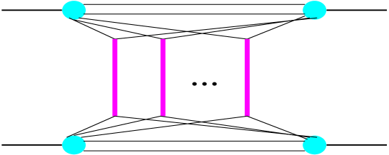
Figure 2: A general multi-pomeron contribution to hadron-hadron scattering amplitude; elementary scattering processes (vertical thick lines) are described as pomeron exchanges.

Correspondingly, hadron $a$ - hadron $d$ elastic scattering amplitude can be obtained summing over any number $n$ of pomeron exchanges [8, 16]:

$$i\,f_{ad}(s,b)=\sum_{j,k}C_{a(j)}\,C_{d(k)}\sum_{n=1}^{\infty}\frac{1}{n!}\int\prod_{l=1}^{n}\left[dx_{l}^{+}dx_{l}^{-}\left(-\lambda_{a(j)}\,\lambda_{d(k)}\,G_{ad}^{\mathbb{P}}(x_{l}^{+}x_{l}^{-}s,b)\right)\right]$$

$$\times N_{a}^{(n)}(x_{1}^{+},\ldots,x_{n}^{+})\,N_{d}^{(n)}(x_{1}^{-},\ldots,x_{n}^{-})\,,$$ (2)

where $s$ and $b$ are c.m. energy squared and impact parameter for the interaction, $G_{ad}^{\mathbb{P}}(x^{+}x^{-}s,b)$ is the un-integrated pomeron exchange eikonal (for fixed values of pomeron light cone momentum shares $x^{\pm}$), and $N_{a}^{(n)}(x_{1},\ldots,x_{n})$ is the light cone momentum distribution of constituent partons - pomeron “ends”. $C_{a(j)}$ and $\lambda_{a(j)}$ are correspondingly relative weights and relative strengths of diffraction eigenstates of hadron $a$ in Good-Walker formalism [17], $\sum_{j}C_{a(j)}=1$, $\sum_{j}C_{a(j)}\lambda_{a(j)}=1$. In particular, two-component picture ($j=1,2$) with one “passive” component, $\lambda_{a(2)}\equiv 0$, corresponds to the usual quasi-eikonal approach [18], with $\lambda_{a(1)}\equiv 1/C_{a(1)}$ being the shower enhancement coefficient.

Assuming a factorized form for $N_{a}^{(n)}$, i.e. $N_{a}^{(n)}(x_{1},\ldots,x_{n})=\prod_{i=1}^{n}N_{a}^{(1)}(x_{i})$, one can simplify (2):

$$f_{ad}(s,b)=i\sum_{j,k}C_{a(j)}\,C_{d(k)}\left[1-e^{-\lambda_{a(j)}\,\lambda_{d(k)}\,\chi_{ad}^{\mathbb{P}}(s,b)}\right]$$ (3)

$$\chi_{ad}^{\mathbb{P}}(s,b)=\int\!dx^{+}dx^{-}\,G_{ad}^{\mathbb{P}}(x^{+}x^{-}s,b)\,N_{a}^{(1)}(x^{+})\,N_{d}^{(1)}(x^{-})\,,$$ (4)

where the vertex $N_{a}^{(1)}(x)$ can be parameterized as $N_{a}^{(1)}(x)\sim x^{-\alpha_{{\rm part}}}(1-x)^{\alpha_{a}^{{\rm lead}}}$, with the parameters $\alpha_{{\rm part}}\simeq 0$, $\alpha_{p}^{{\rm lead}}\simeq 1.5$ related to intercepts of secondary reggeon trajectories [18, 19].

This leads to traditional expressions for total and elastic cross sections and for elastic scattering slope:

$$\sigma_{ad}^{{\rm tot}}(s)=2\,{\rm Im}\int\!\!d^{2}b\,f_{ad}(s,b)=2\sum_{j,k}C_{a(j)}\,C_{d(k)}\int\!\!d^{2}b\;\left[1-e^{-\lambda_{a(j)}\,\lambda_{d(k)}\,\chi_{ad}^{\mathbb{P}}(s,b)}\right]$$ (5)

$$\sigma_{ad}^{{\rm el}}(s)=\int\!\!d^{2}b\;\left[\sum_{j,k}C_{a(j)}\,C_{d(k)}\,\left(1-e^{-\lambda_{a(j)}\,\lambda_{d(k)}\,\chi_{ad}^{\mathbb{P}}(s,b)}\right)\right]^{2}$$ (6)

$$B_{ad}^{{\rm el}}(s)=\left.\frac{d}{dt}\ln\frac{d\sigma_{ad}^{{\rm el}}(s,t)}{dt}\right|_{t=0}=\frac{1}{\sigma_{ad}^{{\rm tot}}(s)}\sum_{j,k}C_{a(j)}\,C_{d(k)}\int\!\!d^{2}b\;b^{2}\;\left[1-e^{-\lambda_{a(j)}\,\lambda_{d(k)}\,\chi_{ad}^{\mathbb{P}}(s,b)}\right],$$ (7)

where $d\sigma_{ad}^{{\rm el}}(s,t)/dt$ is the differential elastic cross section for momentum transfer squared $t$.

In turn, one obtains the cross section for low mass diffractive excitation of the target hadron cutting the elastic scattering diagrams of Fig. 2 in such a way that the cut plane passes between uncut pomerons, with at least one remained on either side of the cut, and selecting in the cut plane elastic intermediate state for hadron $a$ and inelastic one for hadron $d$:

$$\sigma_{ad}^{{\rm LMD(targ)}}(s)=\int\!\!d^{2}b\;\sum_{j,k,l,m}\,C_{a(j)}\,C_{a(l)}\,\left(C_{d(k)}\,\delta_{k}^{m}-C_{d(k)}C_{d(m)}\right)$$

$$\times\left(1-e^{-\lambda_{a(j)}\,\lambda_{d(k)}\,\chi_{ad}^{\mathbb{P}}(s,b)}\right)\;\left(1-e^{-\lambda_{a(l)}\,\lambda_{d(m)}\,\chi_{ad}^{\mathbb{P}}(s,b)}\right).$$ (8)

The projectile single low mass diffraction cross section $\sigma_{ad}^{{\rm LMD(proj)}}(s)$ is obtained via the replacement $(a\longleftrightarrow d)$ in the r.h.s. of (8).

In this scheme the pomeron provides an effective description of a microscopic parton cascade, which mediates the interaction between the projectile and the target hadrons. At moderate energies the underlying parton cascade for the pomeron exchange consists mainly of “soft” partons of small virtualities and can be treated in a purely phenomenological way. The corresponding eikonal can be chosen as [8]

$$G_{ad}^{\mathbb{P}_{{\rm soft}}}(\hat{s},b)=\frac{\gamma_{0}^{2}\,\left(\hat{s}/s_{0}\right)^{\Delta}}{R_{a}^{2}+R_{d}^{2}+\alpha_{\mathbb{P}}^{\prime}(0)\,\ln(\hat{s}/s_{0})}\;\exp\!\left[-\frac{b^{2}}{4\left(R_{a}^{2}+R_{d}^{2}+\alpha_{\mathbb{P}}^{\prime}(0)\,\ln(\hat{s}/s_{0})\right)}\right],$$ (9)

where $s_{0}\simeq 1$ GeV² is the hadronic mass scale, $\Delta=\alpha_{\mathbb{P}}(0)-1$, $\alpha_{\mathbb{P}}(0)$ and $\alpha_{\mathbb{P}}^{\prime}(0)$ are the intercept and the slope of the pomeron Regge trajectory, $R_{a}^{2}$ is the Regge slope of hadron $a$, and $\gamma_{0}$ stands for pomeron coupling to constituent partons.

At higher energies the underlying parton cascade is more and more populated by quarks and gluons of comparatively high virtualities. Dominant contribution comes here from hard scattering of gluons and sea quarks, which are characterized by small fractions $x_{h}^{\pm}$ of parent hadron light cone momenta and are thus preceeded by extended soft parton cascades (“soft pre-evolution”), covering long rapidity intervals, $y_{{\rm soft}}\sim\ln 1/x_{h}^{\pm}$ [2]. One may apply the phenomenological pomeron treatment for the low ($|q^{2}|<Q_{0}^{2}$ ) virtuality part of the cascade and describe parton evolution at higher virtualities $|q^{2}|>Q_{0}^{2}$ using pQCD techniques, $Q_{0}^{2}\sim 1\div 2$ GeV² being a reasonable scale for pQCD being applicable. Thus, a cascade which at least partly develops in the high virtuality region (some $|q^{2}|>Q_{0}^{2}$) can be described as an exchange of a “semi-hard pomeron”, the latter being represented by a piece of QCD ladder sandwiched between two soft pomerons [5, 6], see the 2nd graph in the r.h.s. of Fig. 3.

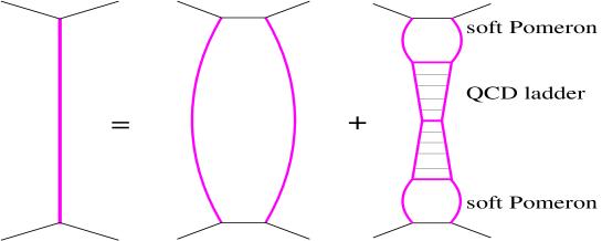
Figure 3: A “general pomeron” (l.h.s.) consists of the soft and semi-hard ones - correspondingly the 1st and the 2nd contributions in the r.h.s.

Thus, the “general pomeron” eikonal is the sum of soft and semi-hard ones, as shown in Fig. 3, and we have [6, 19]

$$G_{ad}^{\mathbb{P}}(\hat{s},b)=G_{ad}^{\mathbb{P}_{{\rm soft}}}(\hat{s},b)+G_{ad}^{\mathbb{P}_{{\rm sh}}}(\hat{s},b)$$ (10)

$$G_{ad}^{\mathbb{P}_{{\rm sh}}}(\hat{s},b)=\frac{1}{2}\sum_{I,J=g,q_{s}}\int\!\!d^{2}b^{\prime}\int\!\frac{dx_{h}^{+}}{x_{h}^{+}}\frac{dx_{h}^{-}}{x_{h}^{-}}\;G_{aI}^{\mathbb{P}_{{\rm soft}}}\!\left(\frac{s_{0}}{x_{h}^{+}},b^{\prime}\right)\,G_{dJ}^{\mathbb{P}_{{\rm soft}}}\!\left(\frac{s_{0}}{x_{h}^{-}},|\vec{b}-\vec{b}^{\prime}|\right)$$

$$\times\sigma_{IJ}^{{\rm QCD}}(x_{h}^{+}\,x_{h}^{-}\,\hat{s},Q_{0}^{2})\,.$$ (11)

Here $\sigma_{IJ}^{{\rm QCD}}(x_{h}^{+}\,x_{h}^{-}\,\hat{s},Q_{0}^{2})$ stands for the contribution of parton ladder with the virtuality cutoff $Q_{0}^{2}$; $I,J$ and $x_{h}^{+},x_{h}^{-}$ are types (gluons and sea quarks) and relative light cone momentum fractions of ladder leg partons:

$$\sigma_{IJ}^{{\rm QCD}}(\hat{s},Q_{0}^{2})=K\sum_{I^{\prime},J^{\prime}}\!\int\!\!dz^{+}dz^{-}\!\!\int\!\!dp_{t}^{2}\;E_{I\rightarrow I^{\prime}}^{{\rm QCD}}(z^{+},Q_{0}^{2},M_{{\rm F}}^{2})\,E_{J\rightarrow J^{\prime}}^{{\rm QCD}}(z^{-},Q_{0}^{2},M_{{\rm F}}^{2})$$

$$\times\frac{d\sigma_{I^{\prime}J^{\prime}}^{2\rightarrow 2}(z^{+}z^{-}\hat{s},p_{t}^{2})}{dp_{t}^{2}}\>\Theta(M_{F}^{2}-Q_{0}^{2})\,,$$ (12)

where $d\sigma_{IJ}^{2\rightarrow 2}/dp_{t}^{2}$ is the differential parton-parton cross section, $p_{t}$ being the parton transverse momentum in the hard process, $M_{F}^{2}$ - the factorization scale (here $M_{F}^{2}=p_{t}^{2}/4$), the factor $K\simeq 1.5$ takes effectively into account higher order QCD corrections, and $E_{I\rightarrow I^{\prime}}^{{\rm QCD}}(z,Q_{0}^{2},Q^{2})$ describes parton evolution from scale $Q_{0}^{2}$ to $Q^{2}$.

The eikonal $G_{aI}^{\mathbb{P}_{{\rm soft}}}(\hat{s},b)$, corresponding to soft pomeron exchange between hadron $a$ and parton $I$, is obtained from (9) replacing one vertex $\gamma_{0}$ by a parameterized pomeron-parton vertex $\gamma_{I}(z),$ $z=s_{0}/\hat{s}$, and neglecting a small slope of pomeron-parton coupling $R_{I}^{2}\sim 1/Q_{0}^{2}$, which gives

$$G_{aI}^{\mathbb{P}_{{\rm soft}}}(\hat{s},b)=\frac{\gamma_{0}\;\gamma_{I}(s_{0}/\hat{s})\;\left(\hat{s}/s_{0}\right)^{\Delta}}{R_{a}^{2}+\alpha_{\mathbb{P}}^{\prime}(0)\,\ln(\hat{s}/s_{0})}\;\exp\!\left[-\frac{b^{2}}{4\left(R_{a}^{2}+\alpha_{\mathbb{P}}^{\prime}(0)\,\ln(\hat{s}/s_{0})\right)}\right].$$ (13)

Here we use [6, 19]

$$\gamma_{g}(z)=r_{g}\,(1-w_{qg})\;(1-z)^{\beta_{g}}$$ (14)

$$\gamma_{q_{s}}(z)=r_{g}\,w_{qg}\int_{z}^{1}\!dy\;y^{\Delta}\;P_{qg}(y)\;(1-z/y)^{\beta_{g}},$$ (15)

where $P_{qg}(y)=3\,[y^{2}+(1-y)^{2}]$ is the usual Altarelli-Parisi splitting kernel for three active flavors. By construction, the eikonal $G_{aI}^{\mathbb{P}_{{\rm soft}}}(s_{0}/x,b)$ describes momentum fraction $x$ and impact parameter $b$ distribution of parton $I$ (gluon or sea quark) in the soft pomeron at virtuality scale $Q_{0}^{2}$, with the constant $r_{g}$ being fixed by parton momentum conservation

$$\int_{0}^{1}\!dx\int\!d^{2}b\;\left[G_{ag}^{\mathbb{P}_{{\rm soft}}}(s_{0}/x,b)+G_{aq_{s}}^{\mathbb{P}_{{\rm soft}}}(s_{0}/x,b)\right]=1\,.$$ (16)

Convoluting $G_{aI}^{\mathbb{P}_{{\rm soft}}}$ with the constituent parton distribution $N_{a}^{(1)}(x)$, one obtains momentum and impact parameter distribution of parton $I$ in hadron $a$ at virtuality scale $Q_{0}^{2}$:

$$x\,\tilde{f}_{I/a}(x,b,Q_{0}^{2})=\int_{x}^{1}\!dx^{\prime}\,N_{a}^{(1)}(x^{\prime})\;G_{aI}^{\mathbb{P}_{{\rm soft}}}\!\left(\frac{s_{0}\,x^{\prime}}{x},b\right).$$ (17)

In addition to $\chi_{ad}^{\mathbb{P}}(s,b)$, defined by (4), (9–11), one may include contributions of valence quark hard interactions with each other or with sea quarks and gluons $\chi_{ad}^{{\rm val-val}}$, $\chi_{ad}^{{\rm val-sea}}$, $\chi_{ad}^{{\rm sea-val}}$ [6, 19]. In case of valence quarks one can neglect the “soft pre-evolution” and use for their momentum and impact parameter distribution at scale $Q_{0}^{2}$

$$\tilde{f}_{q_{v}/a}(x,b,Q_{0}^{2})=\frac{q_{v}(x,Q_{0}^{2})}{4\pi\,R_{a}^{2}}\;\exp\!\left(-\frac{b^{2}}{4R_{a}^{2}}\right),$$ (18)

with $q_{v}(x,Q_{0}^{2})$ being a parameterized input (here GRV94 [21]).

Correspondingly, the complete hadron-hadron interaction eikonal can be written as [6, 19]

$$\chi_{ad}(s,b)=\chi_{ad}^{\mathbb{P}}(s,b)+\chi_{ad}^{{\rm val-val}}(s,b)+\chi_{ad}^{{\rm val-sea}}(s,b)+\chi_{ad}^{{\rm sea-val}}(s,b)$$

$$=\chi_{ad}^{\mathbb{P}_{{\rm soft}}}(s,b)+\frac{K}{2}\sum_{I,J}\!\int\!\!dx^{+}dx^{-}\!\int\!\!dp_{t}^{2}\!\int\!\!d^{2}b^{\prime}\;\tilde{f}_{I/a}(x^{+},b^{\prime},M_{F}^{2})\>\tilde{f}_{J/d}(x^{-},|\vec{b}-\vec{b}^{\prime}|,M_{F}^{2})$$

$$\times\frac{d\sigma_{IJ}^{2\rightarrow 2}(x^{+}x^{-}s,p_{t}^{2})}{dp_{t}^{2}}\>\Theta(M_{F}^{2}-Q_{0}^{2})\,,$$ (19)

where $\chi_{ad}^{\mathbb{P}_{{\rm soft}}}(s,b)=\int\!dx^{+}dx^{-}\,G_{ad}^{\mathbb{P}_{{\rm soft}}}(x^{+}x^{-}s,b)\,N_{a}^{(1)}(x^{+})\,N_{d}^{(1)}(x^{-})$ and parton momentum and impact parameter distributions $\tilde{f}_{I/a}(x,b,Q^{2})$ at arbitrary scale $Q^{2}$ are obtained evolving the input ones (17-18) from $Q_{0}^{2}$ to $Q^{2}$:

$$\tilde{f}_{I/a}(x,b,Q^{2})=\sum_{J=g,q_{s},q_{v}}\!\int_{x}^{1}\!\!\frac{dz}{z}\>E_{J\rightarrow I}^{{\rm QCD}}(z,Q_{0}^{2},Q^{2})\;\tilde{f}_{J/a}(x/z,b,Q_{0}^{2})\,.$$ (20)

It is noteworthy that the eikonal (19) is similar to the usual ansatz (1) of the mini-jet approach, apart from the fact that in the latter case one assumed a factorized momentum and impact parameter dependence of parton distributions, i.e.

$$\tilde{f}_{I/a}^{{\rm mini-jet}}(x,b,Q^{2})=f_{I/a}(x,Q^{2})\;T_{a}^{{\rm e/m}}(b)\,.$$ (21)

In the above-described approach parton distributions at arbitrary scale $Q^{2}$ are obtained from a convolution of “soft” and “hard” parton evolution, the former being described by the soft pomeron asymptotics. As a consequence, partons of smaller virtualities result from a longer “soft” evolution and are distributed over a larger transverse area. On the other hand, the latter circumstance is closely related to the chosen functional form (9) for the pomeron amplitude, characterized by a Gaussian impact parameter dependence. In the mini-jet approach one typically employs a dipole parameterization for hadronic form-factors $T_{a}^{{\rm e/m}}(b)$, which allows to put the slope of the soft contribution down to zero and thus leads to the geometrical scaling picture.

3 Non-linear screening corrections

The above-described picture appears to be incomplete in the “dense” regime, i.e. in the limit of high energies and small impact parameters for the interaction. There, a large number of elementary scattering processes occurs and corresponding underlying parton cascades overlap and interact with each other, giving rise to significant non-linear effects. Here we are going to treat non-linear screening effects in the framework of Gribov’s reggeon scheme [7, 8] by means of enhanced pomeron diagrams, which involve pomeron-pomeron interactions [11, 12]. Concerning multi-pomeron vertices, we assume that they are characterized by small slope $R_{\mathbb{P}}^{2}$ (neglected in the following) and by eikonal structure, i.e. for the vertex which describes the transition of $m$ into $n$ pomerons we use

$$g_{mn}=r_{3\mathbb{P}}\,\gamma_{\mathbb{P}}^{m+n-3}/(4\pi\,m!\,n!)\,,$$ (22)

with $r_{3\mathbb{P}}$ being the triple-pomeron coupling. Doing a replacement $r_{3\mathbb{P}}=4\pi\,G\,\gamma_{\mathbb{P}}^{3}$ and neglecting momentum spread of pomeron “ends” in the vertices, for a pomeron exchanged between two vertices, separated from each other by rapidity $y$ and impact parameter $b$, we use the eikonal $G_{\mathbb{PP}}^{\mathbb{P}}(y,b)$, being the sum of corresponding soft and semi-hard contributions $G_{\mathbb{PP}}^{\mathbb{P}_{{\rm soft}}}(y,b)$, $G_{\mathbb{PP}}^{\mathbb{P}_{{\rm sh}}}(y,b)$. The latter are obtained from $G_{ad}^{\mathbb{P}_{{\rm soft}}}(s_{0}\,e^{y},b)$, $G_{ad}^{\mathbb{P}_{{\rm sh}}}(s_{0}\,e^{y},b)$, defined in (9), (11-13), replacing the vertex factors $\gamma_{a}$, $\gamma_{d}$ by $\gamma_{\mathbb{P}}$ and the slopes $R_{a}^{2}$, $R_{d}^{2}$ by $R_{\mathbb{P}}^{2}\sim 0$:

$$G_{\mathbb{PP}}^{\mathbb{P}}(y,b)=G_{\mathbb{PP}}^{\mathbb{P}_{{\rm soft}}}(y,b)+G_{\mathbb{PP}}^{\mathbb{P}_{{\rm sh}}}(y,b)$$ (23)

$$G_{\mathbb{PP}}^{\mathbb{P}_{{\rm soft}}}(y,b)=\frac{\gamma_{\mathbb{P}}^{2}\;e^{\Delta\,y}}{\alpha_{\mathbb{P}}^{\prime}(0)\,y}\;\exp\!\left[-\frac{b^{2}}{4\alpha_{\mathbb{P}}^{\prime}(0)\,y}\right]$$ (24)

$$G_{\mathbb{PP}}^{\mathbb{P}_{{\rm sh}}}(y,b)=\frac{1}{2}\sum_{I,J}\int\!\!d^{2}b^{\prime}\!\int\!dy^{+}\,dy^{-}\;G_{\mathbb{P}I}^{\mathbb{P}_{{\rm soft}}}(y^{+},b^{\prime})\,G_{\mathbb{P}J}^{\mathbb{P}_{{\rm soft}}}(y^{-},|\vec{b}-\vec{b}^{\prime}|)\,\sigma_{IJ}^{{\rm QCD}}(s_{0}\,e^{y-y^{+}-y^{-}},Q_{0}^{2})$$ (25)

$$G_{\mathbb{P}I}^{\mathbb{P}_{{\rm soft}}}(y,b)=\frac{\gamma_{\mathbb{P}}\;\gamma_{I}(e^{-y})\;e^{\Delta\,y}}{\alpha_{\mathbb{P}}^{\prime}(0)\,y}\,\exp\!\left[-\frac{b^{2}}{4\alpha_{\mathbb{P}}^{\prime}(0)\,y}\right].$$ (26)

Similarly, for a pomeron exchanged between hadron $a$ and a multi-pomeron vertex we use the eikonal $\chi_{a\mathbb{P}}^{\mathbb{P}}(y,b)$, defined as

$$\chi_{a\mathbb{P}}^{\mathbb{P}}(y,b)=\int\!dx\;N_{a}^{(1)}(x)\,\left[G_{a\mathbb{P}}^{\mathbb{P}_{{\rm soft}}}(y-\ln\!\frac{1}{x},b)+G_{a\mathbb{P}}^{\mathbb{P}_{{\rm sh}}}(y-\ln\!\frac{1}{x},b)\right]$$ (27)

$$G_{a\mathbb{P}}^{\mathbb{P}_{{\rm soft}}}(y,b)=\frac{\gamma_{0}\;\gamma_{\mathbb{P}}\;e^{\Delta\,y}}{R_{a}^{2}+\alpha_{\mathbb{P}}^{\prime}(0)\,y}\;\exp\!\left[-\frac{b^{2}}{4\left(R_{a}^{2}+\alpha_{\mathbb{P}}^{\prime}(0)\,y\right)}\right]$$ (28)

$$G_{a\mathbb{P}}^{\mathbb{P}_{{\rm sh}}}(y,b)=\frac{1}{2}\sum_{I,J}\int\!\!d^{2}b^{\prime}\!\int\!dy^{+}\,dy^{-}\;G_{aI}^{\mathbb{P}_{{\rm soft}}}(y^{+},b^{\prime})\;G_{\mathbb{P}J}^{\mathbb{P}_{{\rm soft}}}(y^{-},|\vec{b}-\vec{b}^{\prime}|)\;\sigma_{IJ}^{{\rm QCD}}\!(s_{0}\,e^{y-y^{+}-y^{-}},Q_{0}^{2})\,.$$ (29)

As an example, the contribution of enhanced diagrams with only one multi-pomeron vertex, which are coupled to diffractive eigenstates $j$ and $k$ of hadrons $a$ and $d$, can be obtained using standard reggeon calculus techniques [7, 8, 11, 12]: summing over $m\geq 1$ pomerons exchanged between the vertex and the projectile hadron, $n\geq 1$ pomeron exchanges between the vertex and the target, subtracting the term with $m=n=1$ (pomeron self-coupling), and integrating over rapidity $y_{1}<Y=\ln\frac{s}{s_{0}}$ and impact parameter $\vec{b}_{1}$ of the vertex, as shown in Fig. 4:

$$\chi_{ad(jk)}^{\mathbb{PPP}(1)}\!(s,b)=\frac{G}{\lambda_{a(j)}\,\lambda_{d(k)}}\sum_{m,n\geq 1;m+n\geq 3}\int_{0}^{Y}\!\!dy_{1}\!\int\!\!d^{2}b_{1}\;\frac{\left[-\lambda_{a(j)}\,\chi_{a\mathbb{P}}^{\mathbb{P}}(Y-y_{1},|\vec{b}-\vec{b}_{1}|)\right]^{m}}{m!}$$

$$\times\frac{\left[-\lambda_{d(k)}\,\chi_{d\mathbb{P}}^{\mathbb{P}}(y_{1},b_{1})\right]^{n}}{n!}=\frac{G}{\lambda_{a(j)}\,\lambda_{d(k)}}\int_{0}^{Y}\!\!dy_{1}\!\int\!\!d^{2}b_{1}\,\left\{\left(1-e^{-\lambda_{a(j)}\,\chi_{a\mathbb{P}}^{\mathbb{P}}(Y-y_{1},|\vec{b}-\vec{b}_{1}|)}\right)\right.$$

$$\left.\times\left(1-e^{-\lambda_{d(k)}\,\chi_{d\mathbb{P}}^{\mathbb{P}}(y_{1},b_{1})}\right)-\lambda_{a(j)}\,\lambda_{d(k)}\,\chi_{a\mathbb{P}}^{\mathbb{P}}(Y-y_{1},|\vec{b}-\vec{b}_{1}|)\;\chi_{d\mathbb{P}}^{\mathbb{P}}(y_{1},b_{1})\right\}.$$ (30)

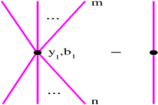
Figure 4: Lowest order enhanced graphs; pomeron connections to the projectile and target hadrons not shown explicitely.

Here our key assumption is that pomeron-pomeron coupling proceeds via partonic processes at comparatively low virtualities, $|q^{2}|<Q_{0}^{2}$, with $Q_{0}$ being a fixed energy-independent parameter [19, 22]. In that case multi-pomeron vertexes involve only interactions between soft pomerons or between “soft ends” of semi-hard pomerons, as shown in Fig. 5; direct coupling between parton ladders in the region of high virtualities $|q^{2}|>Q_{0}^{2}$ is neglected.

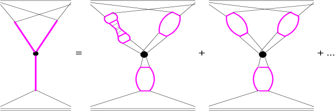
Figure 5: Contributions to the triple-pomeron vertex from interactions between soft and semi-hard pomerons.

As shown in [14], the contribution of dominant enhanced diagrams can be represented by the graphs of Fig. 6.

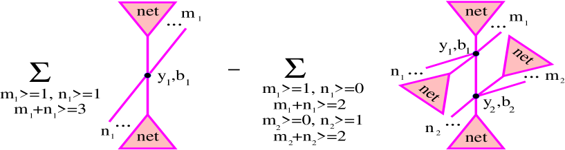
Figure 6: Complete set of dominant enhanced diagrams; $y_{i}$, $\vec{b}_{i}$ ($i=1,2$) denote rapidity and impact parameter positions of multi-pomeron vertices, $i$-th vertex couples together $m_{i}$ projectile and $n_{i}$ target “net fans”.

With our present conventions the corresponding eikonal contribution can be written as

$$\chi_{ad(jk)}^{{\rm enh}}(s,b)=\frac{G}{\lambda_{a(j)}\,\lambda_{d(k)}}\int_{0}^{Y}\!\!dy_{1}\!\int\!\!d^{2}b_{1}\left\{\left[\left(1-e^{-\lambda_{a(j)}\,\chi_{a(j)|d(k)}^{{\rm net}}\!(Y-y_{1},\vec{b}-\vec{b}_{1}|Y,\vec{b})}\right)\right.\right.$$

$$\left.\times\left(1-e^{-\lambda_{d(k)}\,\chi_{d(k)|a(j)}^{{\rm net}}\!(y_{1},\vec{b}_{1}|Y,\vec{b}}\right)-\lambda_{a(j)}\lambda_{d(k)}\,\chi_{a(j)|d(k)}^{{\rm net}}\!(Y-y_{1},\vec{b}-\vec{b}_{1}|Y,\vec{b})\;\chi_{d(k)|a(j)}^{{\rm net}}\!(y_{1},\vec{b}_{1}|Y,\vec{b})\right]$$

$$-G\int_{0}^{y_{1}}\!\!dy_{2}\!\int\!\!d^{2}b_{2}\;G_{\mathbb{PP}}^{\mathbb{P}}(y_{1}-y_{2},|\vec{b}_{1}-\vec{b}_{2}|)\;\left[\left(1-e^{-\lambda_{a(j)}\,\chi_{a(j)|d(k)}^{{\rm net}}\!(Y-y_{1},\vec{b}-\vec{b}_{1}|Y,\vec{b})}\right)\right.$$

$$\left.\times e^{-\lambda_{d(k)}\,\chi_{d(k)|a(j)}^{{\rm net}}\!(y_{1},\vec{b}_{1}|Y,\vec{b})}-\lambda_{a(j)}\,\chi_{a(j)|d(k)}^{{\rm net}}\!(Y-y_{1},\vec{b}-\vec{b}_{1}|Y,\vec{b})\right]$$

$$\left.\times\left[\left(1-e^{-\lambda_{d(k)}\,\chi_{d(k)|a(j)}^{{\rm net}}\!(y_{2},\vec{b}_{2}|Y,\vec{b})}\right)e^{-\lambda_{a(j)}\,\chi_{a(j)|d(k)}^{{\rm net}}\!(Y-y_{2},\vec{b}-\vec{b}_{2}|Y,\vec{b})}-\lambda_{d(k)}\,\chi_{d(k)|a(j)}^{{\rm net}}\!(y_{2},\vec{b}_{2}|Y,\vec{b})\right]\right\}.$$ (31)

Here $\chi_{a(j)|d(k)}^{{\rm net}}\!(y,\vec{b}_{1}|Y,\vec{b})$ stands for the contribution of “net fan” graphs, which correspond to arbitrary “nets” of pomerons, exchanged between hadrons $a$ and $d$ (represented by their diffractive components $j,k$), with one pomeron vertex in the “handle” of the “fan” being fixed; $y$, $b_{1}$ are rapidity and impact parameter distances between hadron $a$ and this vertex. The “net fan” contribution $\chi_{a(j)|d(k)}^{{\rm net}}$ is defined via the recursive equation of Fig. 7 [14]:

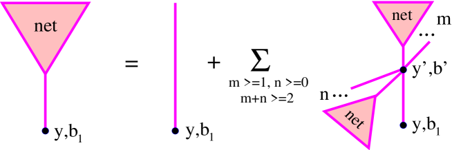
Figure 7: Recursive equation for the projectile “net fan” contribution $\chi_{a(j)|d(k)}^{{\rm net}}\!(y,\vec{b}_{1}|Y,\vec{b})$; $y$, $b_{1}$ are rapidity and impact parameter distances between hadron $a$ and the vertex in the “handle” of the “fan”. The vertex $(y^{\prime},b^{\prime})$ couples together $m$ projectile and $n$ target “net fans”.

$$\chi_{a(j)|d(k)}^{{\rm net}}(y,\vec{b}_{1}|Y,\vec{b})=\chi_{a\mathbb{P}}^{\mathbb{P}}(y,b_{1})+\frac{G}{\lambda_{a(j)}}\int_{0}^{y}\!\!dy^{\prime}\int\!\!d^{2}b^{\prime}\;G_{\mathbb{PP}}^{\mathbb{P}}(y-y^{\prime},|\vec{b}_{1}-\vec{b}^{\prime}|)$$

$$\times\left[\left(1-e^{-\lambda_{a(j)}\,\chi_{a(j)|d(k)}^{{\rm net}}\!(y^{\prime},\vec{b}^{\prime}|Y,\vec{b})}\right)\,e^{-\lambda_{d(k)}\,\chi_{d(k)|a(j)}^{{\rm net}}\!(Y-y^{\prime},\vec{b}-\vec{b}^{\prime}|Y,\vec{b})}-\lambda_{a(j)}\,\chi_{a(j)|d(k)}^{{\rm net}}\!(y^{\prime},\vec{b}^{\prime}|Y,\vec{b})\right].$$ (32)

Thus, one can calculate total, elastic, and single low mass diffraction cross sections, as well as the elastic scattering slope for hadron-hadron scattering, with non-linear screening corrections taken into account, using usual expressions (5-8), with the pomeron eikonal $\chi_{ad}^{\mathbb{P}}$ being replaced by the sum of $\chi_{ad}^{\mathbb{P}}$ and $\chi_{ad(jk)}^{{\rm enh}}$:

$$\chi_{ad(jk)}^{{\rm tot}}(s,b)=\chi_{ad}^{\mathbb{P}}(s,b)+\chi_{ad(jk)}^{{\rm enh}}(s,b)\,.$$ (33)

In addition, considering different unitarity cuts of elastic scattering diagrams of Figs. 2, 6, one can obtain cross sections for various inelastic final states in hadron-hadron interactions, including ones characterized by a rapidity gap signature. While a general analysis of that kind is beyond the scope of the current work and will be presented elsewhere [23], we include in the Appendix a simplified derivation of single high mass diffraction cross section, with the final result being defined by (48-50).

Let us also derive screening corrections to parton (sea quark and gluon) momentum and impact parameter distributions $\tilde{f}_{I/a}(x,b,Q^{2})$, which come from diagrams of “fan” type [1]. In our scheme the general “fan” contribution can be obtained solving iteratively the recursive equation of Fig. 8,

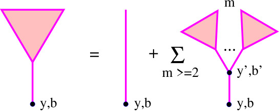
Figure 8: Recursive equation for the projectile “fan” contribution $\chi_{a(j)}^{{\rm fan}}(y,b)$; $y$ and $b$ are rapidity and impact parameter distances between hadron $a$ and the vertex in the “handle” of the “fan”. The vertex $(y^{\prime},b^{\prime})$ couples together $m$ projectile “fans”.

which is a particular case of more general “net fan” equation of Fig. 7, when all intermediate vertices are connected to hadron $a$ only (i.e. $n\equiv 0$ in Fig. 7):

$$\chi_{a(j)}^{{\rm fan}}(y,b)=\chi_{a\mathbb{P}}^{\mathbb{P}}(y,b)+\frac{G}{\lambda_{a(j)}}\int_{0}^{y}\!\!dy^{\prime}\int\!\!d^{2}b^{\prime}\;G_{\mathbb{PP}}^{\mathbb{P}}(y-y^{\prime},|\vec{b}-\vec{b}^{\prime}|)$$

$$\times\left[1-e^{-\lambda_{a(j)}\,\chi_{a(j)}^{{\rm fan}}(y^{\prime},b^{\prime})}-\lambda_{a(j)}\,\chi_{a(j)}^{{\rm fan}}(y^{\prime},b^{\prime})\right].$$ (34)

Then, parton distributions $x\,\tilde{f}_{I/a}^{{\rm scr}}(x,b,Q_{0}^{2})$ ($I=g,q_{s}$) are defined by diagrams of Fig. 8 with $y=-\ln x$ and with the down-most vertices being replaced by the pomeron-parton coupling, which amounts to replace the eikonals $\chi_{a\mathbb{P}}^{\mathbb{P}}(y,b)$, $G_{\mathbb{PP}}^{\mathbb{P}}(y-y^{\prime},|\vec{b}-\vec{b}^{\prime}|)$ in (34) by $x\,\tilde{f}_{I/a}(x,b,Q_{0}^{2})$, $G_{\mathbb{P}I}^{\mathbb{P}_{{\rm soft}}}(-\ln x-y^{\prime},|\vec{b}-\vec{b}^{\prime}|)$ correspondingly, the latter being defined in (17), (26). Thus, averaging over diffraction eigenstates of hadron $a$ with the corresponding weights $C_{a(j)}\lambda_{a(j)}$, we obtain

$$x\,\tilde{f}_{I/a}^{{\rm scr}}(x,b,Q_{0}^{2})=x\,\tilde{f}_{I/a}(x,b,Q_{0}^{2})+G\sum_{j}C_{a(j)}\int_{0}^{-\ln x}\!\!dy^{\prime}\int\!\!d^{2}b^{\prime}\;G_{\mathbb{P}I}^{\mathbb{P}_{{\rm soft}}}(-\ln x-y^{\prime},|\vec{b}-\vec{b}^{\prime}|)$$

$$\times\left[1-e^{-\lambda_{a(j)}\,\chi_{a(j)}^{{\rm fan}}(y^{\prime},b^{\prime})}-\lambda_{a(j)}\,\chi_{a(j)}^{{\rm fan}}(y^{\prime},b^{\prime})\right].$$ (35)

Parton distributions $\tilde{f}_{I/a}^{{\rm scr}}(x,b,Q^{2})$ at arbitrary scale $Q^{2}$ are obtained substituting $\tilde{f}_{J/a}(x,b,Q_{0}^{2})$ in (20) by $\tilde{f}_{J/a}^{{\rm scr}}(x,b,Q_{0}^{2})$ as the initial conditions for sea quarks and gluons.

Let us finally obtain diffractive parton distributions, which are relevant for diffractive deep inelastic scattering reactions, when a large rapidity gap, not covered by secondary particle production, appears in the process. First, we have to obtain the contribution of unitarity cuts of the “fan” diagrams of Fig. 8, which lead to a rapidity gap of size $y_{{\rm gap}}$ between hadron $a$ and the nearest particle produced after the gap. Introducing a generic symbol for the diffractive contribution $2\chi_{a(j)}^{{\rm diffr}}(y,b,y_{{\rm gap}})$ as a “fork” with broken “handle”, applying AGK cutting rules [15] to the 2nd graph in the r.h.s. of Fig. 8, and collecting cut diagrams of diffractive type, we obtain for $2\chi_{a(j)}^{{\rm diffr}}$ the recursive equation shown in Fig. 9:

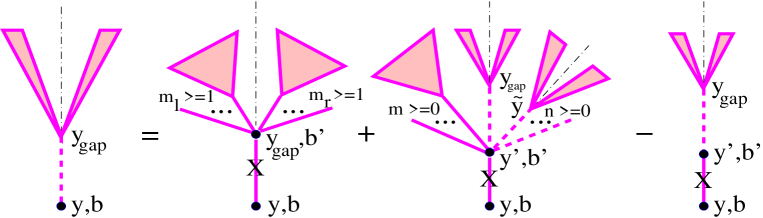
Figure 9: Recursive equation for the diffractive “fan” contribution $\chi_{a(j)}^{{\rm diffr}}(y,b,y_{{\rm gap}})$; $y$, $b$ are rapidity and impact parameter distances between hadron $a$ and the vertex in the “handle” of the “fan”, $y_{{\rm gap}}$ is the size of the rapidity gap. Dot-dashed lines indicate the position of the cut plane; cut pomerons are marked by crosses.

$$2\,\chi_{a(j)}^{{\rm diffr}}(y,b,y_{{\rm gap}})=\frac{G}{\lambda_{a(j)}}\int\!\!d^{2}b^{\prime}\;\left\{\left[1-e^{-\lambda_{a(j)}\,\chi_{a(j)}^{{\rm fan}}(y_{{\rm gap}},b^{\prime})}\right]^{2}\;G_{\mathbb{PP}}^{\mathbb{P}}(y-y_{{\rm gap}},|\vec{b}-\vec{b}^{\prime}|)\right.$$

$$+\int_{y_{{\rm gap}}}^{y}\!\!dy^{\prime}\;2\lambda_{a(j)}\,\chi_{a(j)}^{{\rm diffr}}(y^{\prime},b^{\prime},y_{{\rm gap}})\;G_{\mathbb{PP}}^{\mathbb{P}}(y-y^{\prime},|\vec{b}-\vec{b}^{\prime}|)$$

$$\left.\times\left[\exp\!\left(-2\lambda_{a(j)}\,\chi_{a(j)}^{{\rm fan}}(y^{\prime},b^{\prime})+\int_{y_{{\rm gap}}}^{y^{\prime}}\!\!d\tilde{y}\;2\lambda_{a(j)}\,\chi_{a(j)}^{{\rm diffr}}(y^{\prime},b^{\prime},\tilde{y})\right)-1\right]\right\}.$$ (36)

The first graph in the r.h.s. of Fig. 9 is obtained when the cut plane passes between the “fans” connected to the vertex $(y^{\prime},b^{\prime})$ in Fig. 8 (in which case we have $y^{\prime}=y_{{\rm gap}}$), with any number but at least one “fan” remained on either side of the cut. Correspondingly the 2nd diagram appears when the cut goes through at least one of the “fans”, producing a rapidity gap of size $y_{{\rm gap}}$ inside. Then, the vertex $(y^{\prime},b^{\prime})$ is coupled to the diffractive "fan" $\chi_{a(j)}^{{\rm diffr}}(y^{\prime},b^{\prime},y_{{\rm gap}})$ and to any number $m\geq 0$ of uncut “fans”, each of which may be positioned on either side of the cut. Also, any number $n\geq 0$ of additional diffractively cut “fans” may be connected to this vertex, provided all of them produce rapidity gaps larger than $y_{{\rm gap}}$: $\tilde{y}_{i}\geq y_{{\rm gap}}$, $i=1,...,n$. Finally, the last graph in the r.h.s. of Fig. 9 is to subtract the pomeron self-coupling contribution ($m=n=0$).

In turn, diffractive PDFs $x\,x_{\mathbb{P}}\,f_{I/a}^{{\rm diffr}}(x,x_{\mathbb{P}},Q_{0}^{2})$ are obtained from diagrams of Fig. 9 with $y=-\ln x$, $y_{{\rm gap}}=-\ln x_{\mathbb{P}}$, replacing the down-most vertex by pomeron-parton coupling (replacing the eikonal $G_{\mathbb{PP}}^{\mathbb{P}}$ in (36) by $G_{\mathbb{P}I}^{\mathbb{P}_{{\rm soft}}}$), averaging over diffractive eigenstates of hadron $a$, and integrating over impact parameter $b$:

$$x\,x_{\mathbb{P}}\,f_{I/a}^{{\rm diffr}}(x,x_{\mathbb{P}},Q_{0}^{2})=4\pi G\gamma_{\mathbb{P}}\,x^{-\Delta}\sum_{j}C_{a(j)}\int\!\!d^{2}b^{\prime}\;\left\{\frac{1}{2}\gamma_{I}\!\left(\frac{x}{x_{\mathbb{P}}}\right)\,x_{\mathbb{P}}^{\Delta}\left[1-e^{-\lambda_{a(j)}\,\chi_{a(j)}^{{\rm fan}}(-\ln x_{\mathbb{P}},b^{\prime})}\right]^{2}\right.$$

$$+\int_{-\ln x_{\mathbb{P}}}^{-\ln x}\!\!dy^{\prime}\;\gamma_{I}\!\left(x\,e^{y^{\prime}}\right)\,e^{-\Delta y^{\prime}}\;\lambda_{a(j)}\,\chi_{a(j)}^{{\rm diffr}}(y^{\prime},b^{\prime},-\ln x_{\mathbb{P}})$$

$$\left.\times\left[\exp\!\left(-2\lambda_{a(j)}\,\chi_{a(j)}^{{\rm fan}}(y^{\prime},b^{\prime})+\int_{-\ln x_{\mathbb{P}}}^{y^{\prime}}\!\!d\tilde{y}\;2\lambda_{a(j)}\,\chi_{a(j)}^{{\rm diffr}}(y^{\prime},b^{\prime},\tilde{y})\right)-1\right]\right\}.$$ (37)

At arbitrary scale $Q^{2}$ we thus have

$$f_{I/a}^{{\rm diffr}}(x,x_{\mathbb{P}},Q^{2})=\sum_{J=g,q_{s}}\!\int_{x/x_{\mathbb{P}}}^{1}\!\!\frac{dz}{z}\>E_{J\rightarrow I}^{{\rm QCD}}(z,Q_{0}^{2},Q^{2})\;f_{J/a}^{{\rm diffr}}(x/z,x_{\mathbb{P}},Q_{0}^{2})\,.$$ (38)

It is noteworthy that (37-38) are only applicable for high mass diffraction ($\beta=x/x_{\mathbb{P}}\ll 1$), as at moderate $\beta$ dominant contribution comes from the so-called $q\bar{q}$ diffraction component [24], which is neglected here.

4 Results and discussion

The obtained formulas have been applied to calculate total, elastic, and single diffraction proton-proton cross sections, elastic scattering slope $B_{pp}^{{\rm el}}(s)$, as well as proton inclusive and diffractive SFs $F_{2/p}(x,Q^{2})$, $F_{2/p}^{D(3)}(x,x_{\mathbb{P}},Q^{2})$. The latter are given to leading order as

$$F_{2/p}(x,Q^{2})=\sum_{I=q,\bar{q}}e_{I}^{2}\,x\,f_{I/p}^{{\rm scr}}(x,Q^{2})+F_{2/p}^{(c)}(x,Q^{2})$$ (39)

$$F_{2/p}^{D(3)}(x,x_{\mathbb{P}},Q^{2})=\sum_{I=q,\bar{q}}e_{I}^{2}\,x\,f_{I/p}^{{\rm diffr}}(x,x_{\mathbb{P}},Q^{2})\,.$$ (40)

Here we use $f_{I/p}^{{\rm scr}}(x,Q^{2})=\int\!d^{2}b\;\tilde{f}_{I/p}^{{\rm scr}}(x,b,Q^{2})$, $\tilde{f}_{I/p}^{{\rm scr}}(x,b,Q^{2})$ being defined by (20) with $\tilde{f}_{J/a}^{{\rm scr}}(x,b,Q_{0}^{2})$ (see (35)) as the initial conditions for sea quarks and gluons; $f_{I/p}^{{\rm diffr}}(x,x_{\mathbb{P}},Q^{2})$ are given in (37-38). The charm quark contribution $F_{2/p}^{(c)}(x,Q^{2})$ has been calculated via the photon-gluon fusion process [25], using $m_{c}=1.3$ GeV for the charm quark mass, and neglected in the diffractive structure function. Single diffraction proton-proton cross section has been calculated as a sum of the low and high mass diffraction contributions, $\sigma_{pp}^{{\rm SD}}(s)=2\,\sigma_{pp}^{{\rm LMD(targ)}}(s)+2\,\sigma_{pp}^{{\rm HMD(targ)}}(s,y_{{\rm gap}})$, the two latter being defined in (8), (50) correspondingly. To compare with experimental data, the size of the rapidity gap for the high mass diffraction has been determined from the condition that the quasi-elastically scattered proton looses less than 5% of its energy, $y_{{\rm gap}}=-\ln 0.05$.

Concerning the parameter choice, we used two-component diffraction scheme with one “passive” component, $\lambda_{p(2)}=0$, and with the standard value of the shower enhancement coefficient $\lambda_{p(1)}=1/C_{p(1)}=\sqrt{1.5}$ [18]. It turned out that a reasonable agreement with data could be achieved even for a rather low virtuality cutoff $Q_{0}^{2}=1$ GeV² for semi-hard processes; for the other parameters we obtained $\alpha_{{\rm P}}(0)=1.15$, $\alpha_{{\rm P}}^{\prime}(0)=0.075$ GeV^-2, $\gamma_{p}=5.6$ GeV^-1, $R_{p}^{2}=2.15$ GeV^-2, $\gamma_{\mathbb{P}}=0.5$ GeV^-1, $G=0.18$ GeV², $\beta_{g}=1$, $w_{qg}=0.22$. The results for $\sigma_{pp}^{{\rm tot}}$, $\sigma_{pp}^{{\rm el}}$, $B_{pp}^{{\rm el}}$, and $F_{2/p}$ are plotted in Figs. 10, 11.

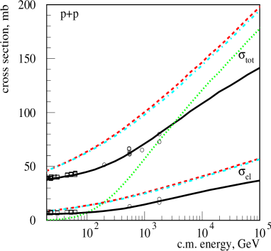
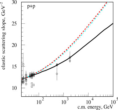
Figure 10: Total and elastic proton-proton cross sections (left) and elastic scattering slope (right) as calculated with (solid lines) and without (dashed and dot-dashed (neglecting valence quark input) lines) enhanced diagram contributions. Dotted line corresponds to $\sigma_{pp}^{{\rm tot}}(s)$, calculated using only the factorized contribution of semi-hard processes $\chi_{pp}^{{\rm sh(fact)}}(s,b)$, as explained in the text. The compilation of data is from [26].

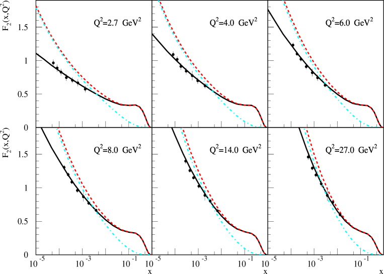
Figure 11: Proton SF $F_{2/p}(x,Q^{2})$ calculated with (solid lines) and without (dashed and dot-dashed (neglecting valence quark input) lines) enhanced graph corrections, compared to data of the ZEUS forward plug calorimeter [27].

For comparison we show also the same quantities, calculated without enhanced diagram contributions, i.e. using the eikonal $\chi_{pp}(s,b)$, given in (19), and the PDFs $\tilde{f}_{I/p}(x,b,Q^{2})$, defined by (20), (17-18). It is noteworthy that our analysis, being devoted to high energy behavior of hadronic cross sections and to the low $x$ asymptotics of SFs, is rather insensitive to input PDFs of valence quarks $q_{v}(x,Q_{0}^{2})$ (see (18)). For the illustration, we repeated the latter calculation neglecting the input valence quark distribution, i.e. setting $q_{v}(x,Q_{0}^{2})\equiv 0$; the results are shown in Figs. 10, 11 by dot-dashed lines. As is easy to see, the obtained variations are very moderate in the range of interest.

In Figs. 12, 13

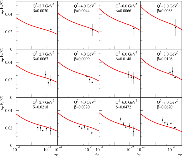
Figure 12: Proton diffractive SF $x_{\mathbb{P}}\,F_{2/p}^{D(3)}(x,x_{\mathbb{P}},Q^{2})$, compared to data of the ZEUS forward plug calorimeter [27].

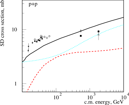
Figure 13: Calculated total, high and low mass single diffraction proton-proton cross sections – solid, dashed, and dotted lines correspondingly. The compilation of data is from [28].

the calculated proton diffractive SF $F_{2/p}^{D(3)}$ and single diffraction proton-proton cross section $\sigma_{pp}^{{\rm SD}}$ are compared to experimental data; the partial contributions of low and high mass diffraction are also shown in Fig. 13. In general, a satisfactory agreement with measurements is observed both for the diffractive DIS contribution and for the “soft” hadronic diffraction. The obtained energy rise of $\sigma_{pp}^{{\rm SD}}(s)$ is somewhat steeper than observed experimentally, due to the rapid increase of the low mass diffraction contribution, as seen in Fig. 13. This is a consequence of using the simple “passive” component (quasi-eikonal) approach, which leads to a proportionality between $\sigma_{ad}^{{\rm el}}$ and $\sigma_{ad}^{{\rm LMD}}$, i.e. $\sigma_{ad}^{{\rm LMD}}(s)/\sigma_{ad}^{{\rm el}}(s)\equiv{\rm const}$, as one can see from (6), (8). Employing a general multi-component scheme with more than one “active” component, one can substantially reduce the energy dependence of the low mass diffraction contribution and improve the agreement with data. It is noteworthy that the obtained moderate energy rise of the high mass diffraction component is not only due to the usual suppression of rapidity gap topologies by the elastic form-factor, but also due to the unitarization of the bare contribution of diffractively cut graphs, which originates from additional re-scattering processes on both projectile and target hadrons; each pomeron, connected to the cut multi-pomeron vertex at the edge of the gap, appears to be a “handle” of either cut or uncut “net fan” sub-graph, as can be seen in Fig. 23.

Let us now note the differences with our previous treatment [14], which used only soft pomeron contributions and was based on the assumption of $\pi$-meson dominance of multi-pomeron vertices. Here, considering contributions of both soft and semi-hard processes and assuming a small slope of multi-pomeron vertices, we obtained an unusually small value for the soft pomeron slope. This is because the enhanced diagram contribution $\chi_{ad(jk)}^{{\rm enh}}(s,b)$, defined in (31), is most significant in the region of comparatively small impact parameters, being characterized by a somewhat smaller effective slope than the one of the soft pomeron. On the other hand, the obtained values of the pomeron intercept $\alpha_{{\rm P}}(0)=1.15$ and of the triple-pomeron coupling $r_{3\mathbb{P}}=4\pi\,G\,\gamma_{\mathbb{P}}^{3}\simeq 0.28$ GeV^-1 are not too different from the ones in [14]: 1.18 and 0.18 GeV^-1 correspondingly.

We would like to stress also an important feature of the presented approach: the full interaction eikonal (33), which includes the enhanced diagram contribution (31), can no longer be expressed in the usual factorized form (1), (19). In particular, non-linear screening corrections to the contribution of semi-hard processes can not be simply absorbed into the re-defined PDFs $\tilde{f}_{I/a}^{{\rm scr}}(x,b,Q^{2})$. Significant non-factorizable corrections come from graphs where at least one pomeron is exchanged in parallel to the hardest parton scattering process, with the simplest example given by the 1st diagram in the r.h.s. of Fig. 5. In fact, such contributions play an important role for reaching the consistency between total hadronic cross sections and structure functions. For the illustration, in Fig. 10 shown also the result for $\sigma_{pp}^{{\rm tot}}(s)$, as calculated using only the factorized semi-hard contribution $\chi_{pp}^{{\rm sh(fact)}}(s,b)$, i.e. using the eikonal (19) with $\chi_{pp}^{\mathbb{P}_{{\rm soft}}}(s,b)\equiv 0$ and with the PDFs $\tilde{f}_{I/p}(x,b,Q^{2})$ being replaced by $\tilde{f}_{I/p}^{{\rm scr}}(x,b,Q^{2})$. It is easy to see that in such a case the cross section rises with energy much faster than obtained before with the full eikonal (33), even though the contribution of soft processes is neglected.

To additionally clarify this point, let us consider PDFs in the low $x$ limit, sketched in Fig. 14,

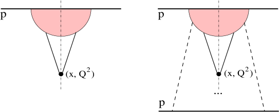
Figure 14: Schematic view of parton distributions as "seen" in DIS (left) and in proton-proton collision (right). Low $x$ parton (sea quark or gluon) originates from the initial state “blob” and interacts with a highly virtual “probe”. In proton-proton interaction the initial “blob” itself is affected by the collision process – due to additional soft re-scatterings on the target, indicated by dashed lines.

as “seen” in DIS reactions and in hadronic collisions. In the former case, depicted on the left, all non-linear corrections to parton dynamics come from re-scattering on constituent partons of the same parent hadron, being hidden in the upper “blob” in the Figure. The corresponding PDFs are thus described by “fan” diagram contributions. On the other hand, in hadron-hadron interaction one encounters additional re-scatterings on constituent partons of the partner hadron, indicated symbolically in the r.h.s. graph of Fig. 14 as dashed lines connecting the upper “blob” with the target hadron. Parton cascades, which mediate these additional re-scattering processes, may couple both to independent constituents of the projectile hadron, which would lead to the usual multiple scattering picture of Fig. 2, or to “soft” parents of the given high-$p_{t}$ parton, as shown in Fig. 1(right), thus modifying the initial state parton evolution. In the high energy asymptotics the second configuration dominates, being enhanced by logarithmic factors. As a consequence, both the interaction eikonal and correspondingly the cross sections for particular inelastic final states can not be expressed via universal PDFs of free hadrons. In principle, this is not surprising, keeping in mind that QCD collinear factorization holds only for fully inclusive quantities [29]. In the present approach such initial state “blobs”, with the re-scatterings included, are described by the “net fan” contributions. The latter may be regarded as a kind of reaction-dependent “parton distributions”, which are probed during interaction and are thus affected by the surrounding medium.

At the same moment, due to the AGK cancellations [15], the above-discussed non-factorizable graphs give negligible contribution to inclusive high-$p_{t}$ jet cross sections. Single inclusive particle spectra are defined as usual by the diagrams of Fig. 15 [30],

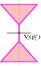
Figure 15: Diagrams contributing to single inclusive cross sections; $V_{c}(\vec{p}_{c})$ is the particle $c$ emission vertex from a cut pomeron.

as far as higher twist effects due to final high-$p_{t}$ parton re-scattering are neglected [31]. In particular, inclusive jet cross sections are thus given in the usual factorized form [32]: as the convolution of hadronic PDFs $f_{I(J)/a(d)}^{{\rm scr}}(x^{+(-)},Q^{2})$ and matrix elements for parton emission.

It is noteworthy that the presented results have been obtained under the assumption on the eikonal structure (22) of multi-pomeron vertices. In principle, one may restrict himself with only triple-pomeron vertices, i.e. set $\gamma_{\mathbb{P}}=0$ in (22). In practical terms this would mean to replace the constant $G$ by $r_{3\mathbb{P}}/(4\pi\,\gamma_{\mathbb{P}}^{3})$ and to consider the limit $\gamma_{\mathbb{P}}\rightarrow 0$ in all the obtained formulas. However, in such a case the scheme would be incomplete: one will need to include also the contributions of pomeron “loop” diagrams, which contain internal multi-pomeron vertices connected to each other by at least two pomerons. In the eikonal scheme these contributions are suppressed by exponential factors [12, 14], which allowed to neglect them in the present analysis.

It is also worth reminding that throughout this work we neglected the effects of pomeron-pomeron coupling in high ($|q|^{2}>Q_{0}^{2}$) virtuality region. One may expect that in very high energy asymptotics those contributions also become significant. However, being suppressed as $1/q^{4}$, they should manifest themselves only in the sufficiently “black” region of moderately small impact parameters, where parton densities are high enough to compensate the mentioned suppression. Therefore, we do not expect a significant modification of the cross section results obtained, when such contributions are taken into account.

In conclusion, accounting for non-linear screening effects, one can obtain a consistent description of hadronic cross sections and of corresponding structure functions, using a fixed energy-independent virtuality cutoff for the contribution of semi-hard processes. On the other hand, a general consistency is observed between “soft” hadronic diffraction and the one measured in DIS processes. An important feature of the proposed scheme is that the contribution of semi-hard processes to the interaction eikonal contains a significant non-factorizable part. This circumstance has to be taken into account if one attempts to extract information on parton saturation from the behavior of hadronic cross sections. On the other hand, by virtue of the AGK cancellations the corresponding diagrams do not contribute to inclusive parton jet spectra and the scheme preserves the QCD factorization picture.

Appendix

We are going to derive contributions of diffractive cuts of general enhanced graphs of Fig. 6. It is convenient to start from the analysis of unitarity cuts of “net fan” diagrams of Fig. 7. One can separate them in two classes: in the first sub-set cut pomerons form a “fan”-like structure, some examples shown in Fig. 16 (a), (b), (c);

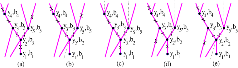
Figure 16: Examples of graphs obtained by cutting the same projectile “net fan” diagram: in the graphs (a), (b), (c) we have a “fan”-like structure of cut pomerons (marked by crosses); in the diagrams (d), (e) the cut pomeron exchanged between the vertex ($y_{3},b_{3}$) and the target forms a “zig-zag” with the “handle” of the “fan”. The cut plane is indicated by dot-dashed lines.

in the diagrams of the second kind some intermediate vertices contain cut pomerons connected to the partner hadron $d$, see Fig. 16 (d), (e), such that these pomerons are arranged in a “zig-zag” way with respect to the “handle” of the “fan”.

Let us consider the first class and obtain separately both the total contribution of “fan”-like cuts $2\bar{\chi}_{a(j)|d(k)}^{{\rm fan}}$ and a part of it, formed by diagrams with the “handle” of the “fan” being uncut (see Fig. 16 (b)) - $2\tilde{\chi}_{a(j)|d(k)}^{{\rm fan}}$. Applying AGK cutting rules [15] to the general “net fan” graphs of Fig. 7 and collecting contributions of cuts of desirable structures we obtain for $2\bar{\chi}_{a(j)|d(k)}^{{\rm fan}}-2\tilde{\chi}_{a(j)|d(k)}^{{\rm fan}}$, $2\tilde{\chi}_{a(j)|d(k)}^{{\rm fan}}$ the representations of Figs. 17, 18,

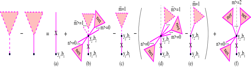
Figure 17: Recursive equation for the contribution $2\bar{\chi}_{a(j)|d(k)}^{{\rm fan}}-2\tilde{\chi}_{a(j)|d(k)}^{{\rm fan}}$ of “fan”-like cuts of “net-fan” diagrams, where the cut plane goes through the “handle” of the “fan”. Cut pomerons are marked by crosses, the cut plane is indicated by dot-dashed lines.

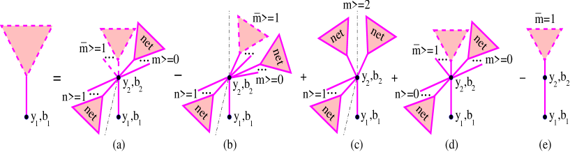
Figure 18: Recursive equation for the contribution $2\tilde{\chi}_{a(j)|d(k)}^{{\rm fan}}$ of “fan”-like cuts of “net-fan” diagrams, where the “handle” of the “fan” remains uncut. Cut pomerons are marked by crosses, the cut plane is indicated by dot-dashed lines.

which gives

$$2\,\bar{\chi}_{a(j)|d(k)}^{{\rm fan}}(y_{1},\vec{b}_{1}|Y,\vec{b})-2\,\tilde{\chi}_{a(j)|d(k)}^{{\rm fan}}(y_{1},\vec{b}_{1}|Y,\vec{b})=2\,\chi_{a\mathbb{P}}^{\mathbb{P}}(y_{1},b_{1})+\frac{G}{\lambda_{a(j)}}\int_{0}^{y_{1}}\!\!dy_{2}\int\!\!d^{2}b_{2}$$

$$\times G_{\mathbb{PP}}^{\mathbb{P}}(y_{1}-y_{2},|\vec{b}_{1}-\vec{b}_{2}|)\;\left\{\left(e^{2\lambda_{a(j)}\,\bar{\chi}_{a(j)|d(k)}^{{\rm fan}}}-1\right)e^{-2\lambda_{a(j)}\,\chi_{a(j)|d(k)}^{{\rm net}}-2\lambda_{d(k)}\,\chi_{d(k)|a(j)}^{{\rm net}}}\right.$$

$$-2\lambda_{a(j)}\,\bar{\chi}_{a(j)|d(k)}^{{\rm fan}}-2\left[\left(e^{\lambda_{a(j)}\,\tilde{\chi}_{a(j)|d(k)}^{{\rm fan}}}-1\right)e^{-\lambda_{a(j)}\,\chi_{a(j)|d(k)}^{{\rm net}}-2\lambda_{d(k)}\,\chi_{d(k)|a(j)}^{{\rm net}}}-\lambda_{a(j)}\,\tilde{\chi}_{a(j)|d(k)}^{{\rm fan}}\right]$$

$$\left.+\left(1-e^{-\lambda_{a(j)}\,\chi_{a(j)|d(k)}^{{\rm net}}}\right)^{2}\,e^{-2\lambda_{d(k)}\,\chi_{d(k)|a(j)}^{{\rm net}}}\right\}$$ (41)

$$2\,\tilde{\chi}_{a(j)|d(k)}^{{\rm fan}}(y_{1},\vec{b}_{1}|Y,\vec{b})=\frac{G}{\lambda_{a(j)}}\int_{0}^{y_{1}}\!\!dy_{2}\int\!\!d^{2}b_{2}\;G_{\mathbb{PP}}^{\mathbb{P}}(y_{1}-y_{2},|\vec{b}_{1}-\vec{b}_{2}|)$$

$$\times\left\{\left(1-e^{-\lambda_{d(k)}\,\chi_{d(k)|a(j)}^{{\rm net}}}\right)e^{-\lambda_{d(k)}\,\chi_{d(k)|a(j)}^{{\rm net}}}\;\left[\left(e^{2\lambda_{a(j)}\,\bar{\chi}_{a(j)|d(k)}^{{\rm fan}}}-1\right)e^{-2\lambda_{a(j)}\,\chi_{a(j)|d(k)}^{{\rm net}}}\right.\right.$$

$$\left.-2\left(e^{\lambda_{a(j)}\,\tilde{\chi}_{a(j)|d(k)}^{{\rm fan}}}-1\right)e^{-\lambda_{a(j)}\,\chi_{a(j)|d(k)}^{{\rm net}}}+\left(1-e^{-\lambda_{a(j)}\,\chi_{a(j)|d(k)}^{{\rm net}}}\right)^{2}\right]$$

$$\left.+2\left[\left(e^{\lambda_{a(j)}\,\tilde{\chi}_{a(j)|d(k)}^{{\rm fan}}}-1\right)e^{-\lambda_{a(j)}\,\chi_{a(j)|d(k)}^{{\rm net}}-\lambda_{d(k)}\,\chi_{d(k)|a(j)}^{{\rm net}}}-\lambda_{a(j)}\,\tilde{\chi}_{a(j)|d(k)}^{{\rm fan}}\right]\right\}.$$ (42)

Here the arguments of the eikonals in the r.h.s. of (41), (42) are understood as $X_{a(j)|d(k)}=X_{a(j)|d(k)}(y_{2},\vec{b}_{2}|Y,\vec{b})$, $X_{d(k)|a(j)}=X_{d(k)|a(j)}(Y-y_{2},\vec{b}-\vec{b}_{2}|Y,\vec{b})$; $X=\chi^{{\rm net}}$, $\bar{\chi}^{{\rm fan}}$, $\tilde{\chi}^{{\rm fan}}$. The first diagram in the r.h.s. of Fig. 17 is obtained cutting the single pomeron exchanged between hadron $a$ and the vertex $(y_{1},b_{1})$ in the r.h.s. of Fig. 7, whereas the other diagrams emerge when the 2nd graph in the r.h.s. of Fig. 7 is cut in such a way that all cut pomerons are arranged in a “fan”-like structure and the cut plane passes through the “handle” of the “fan”. In graph (b) the vertex $(y_{2},b_{2})$ couples together $\bar{m}\geq 1$ cut projectile “net fans”, each one characterized by a “fan”-like structure of cuts, and any numbers $m,n\geq 0$ of uncut projectile and target “net fans”. Here one has to subtract pomeron self-coupling contribution ($\bar{m}=1$; $m,n=0$) - graph (c), as well as the contributions of graphs (d), (e), where in all $\bar{m}$ cut “fans”, connected to the vertex $(y_{2},b_{2})$, the “handles” of the “fans” remain uncut and all these “handles” and all the $m$ uncut projectile “net fans” are situated on the same side of the cut plane. Finally, in graph (f) the cut plane passes between $m\geq 2$ uncut projectile “net fans”, with at least one remained on either side of the cut. In the recursive representation of Fig. 18 for the contribution $2\tilde{\chi}_{a(j)|d(k)}^{{\rm fan}}$ the graphs (a), (b), (c) in the r.h.s. of the Figure are similar to the diagrams (b), (d), (f) of Fig. 17 correspondingly, with the difference that the “handle” of the “fan” is now uncut. Therefore, there are $n\geq 1$ uncut target “net fans” connected to the vertex $(y_{2},b_{2})$, such that at least one of the latter is positioned on the opposite side of the cut plane with respect to the “handle” pomeron. On the other hand, one has to add graph (d), where the vertex $(y_{2},b_{2})$ couples together $\bar{m}\geq 1$ projectile “net fans”, which are cut in a “fan”-like way and have their “handles” uncut and positioned on the same side of the cut plane, together with any numbers $m\geq 0$ of projectile and $n\geq 0$ of target uncut “net fans”, such that the vertex $(y_{2},b_{2})$ remains uncut. Here one has to subtract the pomeron self-coupling ($\bar{m}=1$; $m,n=0$) - graph (e).

Adding (42) to (41), we obtain

$$2\,\bar{\chi}_{a(j)|d(k)}^{{\rm fan}}(y_{1},\vec{b}_{1}|Y,\vec{b})=2\,\chi_{a\mathbb{P}}^{\mathbb{P}}(y_{1},b_{1})+\frac{G}{\lambda_{a(j)}}\int_{0}^{y_{1}}\!\!dy_{2}\int\!\!d^{2}b_{2}\;G_{\mathbb{PP}}^{\mathbb{P}}(y_{1}-y_{2},|\vec{b}_{1}-\vec{b}_{2}|)$$

$$\times\left\{\left[\left(e^{2\lambda_{a(j)}\,\bar{\chi}_{a(j)|d(k)}^{{\rm fan}}}-1\right)e^{-2\lambda_{a(j)}\,\chi_{a(j)|d(k)}^{{\rm net}}}+\left(1-e^{-\lambda_{a(j)}\,\chi_{a(j)|d(k)}^{{\rm net}}}\right)^{2}\right]\,e^{-\lambda_{d(k)}\,\chi_{d(k)|a(j)}^{{\rm net}}}\right.$$

$$\left.-2\lambda_{a(j)}\,\bar{\chi}_{a(j)|d(k)}^{{\rm fan}}\right\}.$$ (43)

Comparing with (32), we see that the solution of (43) is

$$\bar{\chi}_{a(j)|d(k)}^{{\rm fan}}(y_{1},\vec{b}_{1}|Y,\vec{b})\equiv\chi_{a(j)|d(k)}^{{\rm net}}(y_{1},\vec{b}_{1}|Y,\vec{b}).$$ (44)

Correspondingly, using (44), we can simplify (42) to obtain

$$\tilde{\chi}_{a(j)|d(k)}^{{\rm fan}}(y_{1},\vec{b}_{1}|Y,\vec{b})=\frac{G}{\lambda_{a(j)}}\int_{0}^{y_{1}}\!\!dy_{2}\int\!\!d^{2}b_{2}\;G_{\mathbb{PP}}^{\mathbb{P}}(y_{1}-y_{2},|\vec{b}_{1}-\vec{b}_{2}|)\,\left\{\left(1-e^{-\lambda_{a(j)}\,\chi_{a(j)|d(k)}^{{\rm net}}}\right)\right.$$

$$\left.\times e^{-\lambda_{d(k)}\,\chi_{d(k)|a(j)}^{{\rm net}}}-\left(1-e^{\lambda_{a(j)}\,\tilde{\chi}_{a(j)|d(k)}^{{\rm fan}}-\lambda_{a(j)}\,\chi_{a(j)|d(k)}^{{\rm net}}}\right)\,e^{-2\lambda_{d(k)}\,\chi_{d(k)|a(j)}^{{\rm net}}}-\lambda_{a(j)}\,\tilde{\chi}_{a(j)|d(k)}^{{\rm fan}}\right\}.$$ (45)

As the summary contribution of all cuts of “net fan” graphs should be equal to twice the uncut one $2\chi_{a(j)|d(k)}^{{\rm net}}$ (the total discontinuity of an elastic scattering amplitude equals to twice the imaginary part of the amplitude), from (44) we can conclude that contributions of different “zig-zag” cuts of “net fan” graphs (see the examples in Fig. 16 (d), (e)) cancel each other, which can be also verified explicitely [23]. Moreover, it is possible to show that a similar cancellation takes place for all unitarity cuts of the graphs of Fig. 6, which give rise to “zig-zag” sub-structures formed by cut pomerons, and that such cuts do not contribute to diffractive topologies [23]. As an illustration, let us compare the two diagrams in Fig. 19,

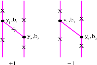
Figure 19: Lowest order cut diagrams of “zig-zag” type; cut pomerons are marked by crosses. Numbers below the graphs indicate relative weights of the corresponding contributions.

whose contributions are equal up to a sign and precisely cancel each other. The right-hand graph provides a screening correction to the eikonal configuration with two cut pomerons. On the other hand, the left-hand graph introduces a new process, with the weight being equal to the one of the screening correction above, and with the particle production pattern being almost identical to the previous two cut pomeron configuration; the only difference arises from the cut pomeron exchanged between the vertices ($y_{1},b_{1}$) and ($y_{2},b_{2}$), which leads to additional particle production in the rapidity interval $[y_{1},y_{2}]$. However, this interval is already covered by particles, which result from the left-most cut pomeron in the two graphs. Correspondingly, the rapidity gap structure of the event remains unchanged.

Thus, in the following we shall restrict ourselves to the analysis of “tree”-like cuts of the diagrams of Fig. 6, whose contributions can be expressed via the ones of “fan”-like cuts of “net fan” graphs. Before we proceed further, let us calculate the contributions of sub-samples of “fan”-like cuts of “net fan” graphs, which give rise to a rapidity gap of size $\geq y_{{\rm gap}}$ between hadron $a$ and the nearest particle produced after the gap, an example shown in Fig. 16 (c) ($y_{{\rm gap}}=y_{4}$). For simplicity, we shall use the two component Good-Walker approach with one passive component, $\lambda_{a(2)}\equiv 0$, $C_{a(1)}\equiv 1/\lambda_{a(1)}$, and neglect sub-dominant contributions of diffractive cuts which leave the “handle” of the “fan” uncut (general derivation proceeds identically).

For the contribution of “fan”-like diffractive cuts $2\bar{\chi}_{a(1)|d(1)}^{{\rm gap}}$ we can easily obtain, similarly to Fig. 9, the recursive representation of Fig. 20,

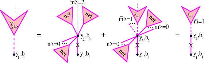
Figure 20: Recursive equation for the contribution $2\bar{\chi}_{a(1)|d(1)}^{{\rm gap}}$ of “fan”-like diffractive cuts of “net-fan” diagrams. Cut pomerons are marked by crosses, the cut plane is indicated by dot-dashed lines.

which gives

$$2\,\bar{\chi}_{a(1)|d(1)}^{{\rm gap}}(y_{1},\vec{b}_{1},y_{{\rm gap}}|Y,\vec{b})=\frac{G}{\lambda_{a(1)}}\int_{y_{{\rm gap}}}^{y_{1}}\!\!dy_{2}\int\!\!d^{2}b_{2}\;G_{\mathbb{PP}}^{\mathbb{P}}(y_{1}-y_{2},|\vec{b}_{1}-\vec{b}_{2}|)$$

$$\times\left\{\left[\left(1-e^{-\lambda_{a(1)}\,\chi_{a(1)|d(1)}^{{\rm net}}(y_{2},\vec{b}_{2}|Y,\vec{b})}\right)^{2}+\left(e^{2\lambda_{a(1)}\,\bar{\chi}_{a(1)|d(1)}^{{\rm gap}}(y_{2},\vec{b}_{2},y_{{\rm gap}}|Y,\vec{b})}-1\right)\right.\right.$$

$$\left.\left.\times e^{-2\lambda_{a(1)}\,\chi_{a(1)|d(1)}^{{\rm net}}(y_{2},\vec{b}_{2}|Y,\vec{b})}\right]e^{-2\lambda_{d(1)}\,\chi_{d(1)|a(1)}^{{\rm net}}(Y-y_{2},\vec{b}-\vec{b}_{2}|Y,\vec{b})}-2\lambda_{a(1)}\,\bar{\chi}_{a(1)|d(1)}^{{\rm gap}}(y_{2},\vec{b}_{2},y_{{\rm gap}}|Y,\vec{b})\right\}.$$ (46)

It is useful to obtain an alternative representation for $2\bar{\chi}_{a(1)|d(1)}^{{\rm gap}}$, considering explicitely all couplings of uncut “net fans” to the “handle” of the diffractively cut “net fan” (see Fig. 21):

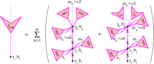
Figure 21: Alternative representation for the contribution $2\bar{\chi}_{a(1)|d(1)}^{{\rm gap}}$ of “fan”-like diffractive cuts of “net-fan” diagrams. The cut pomeron, exchanged between the vertices ($y_{1},b_{1}$) and ($y_{k},b_{k}$), may contain any number $k-2\geq 0$ of intermediate vertices, each one connected to $m_{i}$ projectile and $n_{i}$ target “net fans”; $m_{i},n_{i}\geq 0$, $m_{i}+n_{i}\geq 1$, $i=2,...,k-1$.

$$2\,\bar{\chi}_{a(1)|d(1)}^{{\rm gap}}(y_{1},\vec{b}_{1},y_{{\rm gap}}|Y,\vec{b})=\sum_{k=2}^{\infty}\frac{G^{k-1}}{\lambda_{a(1)}}\;\prod_{i=2}^{k}\left[\int_{y_{{\rm gap}}}^{y_{i-1}}\!\!dy_{i}\int\!\!d^{2}b_{i}\;G_{\mathbb{PP}}^{\mathbb{P}}(y_{i-1}-y_{i},|\vec{b}_{i-1}-\vec{b}_{i}|)\right]$$

$$\times\prod_{j=2}^{k-1}\left[e^{-2\lambda_{a(1)}\,\chi_{a(1)|d(1)}^{{\rm net}}(y_{j},\vec{b}_{j}|Y,\vec{b})-2\lambda_{d(1)}\,\chi_{d(1)|a(1)}^{{\rm net}}(Y-y_{j},\vec{b}-\vec{b}_{j}|Y,\vec{b})}-1\right]e^{-2\lambda_{d(1)}\,\chi_{d(1)|a(1)}^{{\rm net}}(Y-y_{k},\vec{b}-\vec{b}_{k}|Y,\vec{b})}$$

$$\times\left[\left(1-e^{-\lambda_{a(1)}\,\chi_{a(1)|d(1)}^{{\rm net}}(y_{k},\vec{b}_{k}|Y,\vec{b})}\right)^{2}+\left(e^{2\lambda_{a(1)}\,\bar{\chi}_{a(1)|d(1)}^{{\rm gap}}(y_{k},\vec{b}_{k},y_{{\rm gap}}|Y,\vec{b})}-1\right)\right.$$

$$\left.\times e^{-2\lambda_{a(1)}\,\chi_{a(1)|d(1)}^{{\rm net}}(y_{k},\vec{b}_{k}|Y,\vec{b})}\right].$$ (47)

Now we can obtain contributions of diffractive cuts of the diagrams of Fig. 6, using (47) and Fig. 21 to correct for double counting of some graphs in the same manner as in [14] for elastic scattering diagrams. In particular, for the process of central diffraction, separated from the projectile and the target by rapidity gaps of sizes larger or equal to $y_{{\rm gap(1)}}$ and $y_{{\rm gap(2)}}$ correspondingly, we have (see Fig. 22):

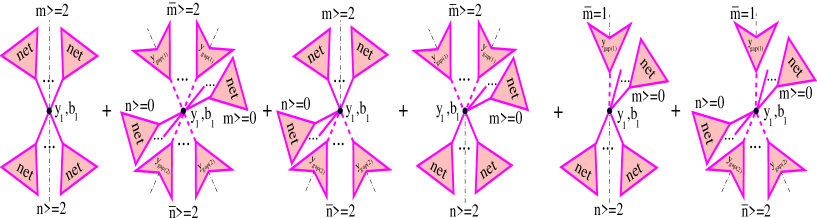
Figure 22: Cut enhanced graphs of double rapidity gap topology.

$$2\,\chi_{ad(11)}^{{\rm 2-gap}}\!(s,b,y_{{\rm gap(1)}},y_{{\rm gap(2)}})=\frac{G}{2\lambda_{a(1)}\,\lambda_{d(1)}}\int_{y_{{\rm gap(2)}}}^{Y-y_{{\rm gap(1)}}}\!\!dy_{1}\!\int\!\!d^{2}b_{1}$$

$$\times\left[\left(1-e^{-\lambda_{a(1)}\,\chi_{a(1)|d(1)}^{{\rm net}}}\right)^{2}+\left(e^{2\lambda_{a(1)}\,\bar{\chi}_{a(1)|d(1)}^{{\rm gap}}}-1\right)e^{-2\lambda_{a(1)}\,\chi_{a(1)|d(1)}^{{\rm net}}}\right]$$

$$\times\left[\left(1-e^{-\lambda_{d(1)}\,\chi_{d(1)|a(1)}^{{\rm net}}}\right)^{2}+\left(e^{2\lambda_{d(1)}\,\bar{\chi}_{d(1)|a(1)}^{{\rm gap}}}-1-2\lambda_{d(1)}\,\bar{\chi}_{d(1)|a(1)}^{{\rm gap}}\right)e^{-2\lambda_{d(1)}\,\chi_{d(1)|a(1)}^{{\rm net}}}\right].$$ (48)

Here the arguments of the eikonals in the r.h.s. of (48) are understood as $\bar{\chi}_{a(1)|d(1)}^{{\rm gap}}=\bar{\chi}_{a(1)|d(1)}^{{\rm gap}}(Y-y_{1},\vec{b}-\vec{b}_{1},y_{{\rm gap(1)}}|Y,\vec{b})$, $\bar{\chi}_{d(1)|a(1)}^{{\rm gap}}=\bar{\chi}_{d(1)|a(1)}^{{\rm gap}}(y_{1},\vec{b}_{1},y_{{\rm gap(2)}}|Y,\vec{b})$, $\chi_{a(1)|d(1)}^{{\rm net}}=\chi_{a(1)|d(1)}^{{\rm net}}(Y-y_{1},\vec{b}-\vec{b}_{1}|Y,\vec{b})$, $\chi_{d(1)|a(1)}^{{\rm net}}=\chi_{d(1)|a(1)}^{{\rm net}}(y_{1},\vec{b}_{1}|Y,\vec{b})$. It is easy to verify that for $y_{{\rm gap(1)}}=y_{{\rm gap(2)}}$ the expression (48) is symmetric under the replacement $(a\longleftrightarrow d)$, which can be made obvious if we expand the projectile diffractively cut “fan” $\bar{\chi}_{a(1)|d(1)}^{{\rm gap}}$ in the last two graphs of Fig. 22 using the relation of Fig. 21.

In turn, requiring at least one rapidity gap of size $\geq y_{{\rm gap}}$ between the projectile hadron and the nearest hadron produced after the gap, we obtain the set of diagrams of Fig. 23,

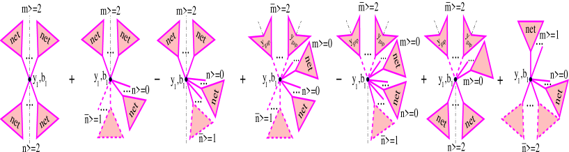
Figure 23: Cut enhanced graphs of target diffraction topology: projectile hadron is separated from other secondary particles by a large rapidity gap.

which gives

$$2\,\chi_{ad(11)}^{{\rm 1-gap}}\!(s,b,y_{{\rm gap}})=\frac{G}{\lambda_{a(1)}\,\lambda_{d(1)}}\int_{0}^{Y-y_{{\rm gap}}}\!\!dy_{1}\!\int\!\!d^{2}b_{1}\;\left\{\left[\left(1-e^{-\lambda_{a(1)}\,\chi_{a(1)|d(1)}^{{\rm net}}}\right)^{2}\right.\right.$$

$$\left.+\left(e^{2\lambda_{a(1)}\,\bar{\chi}_{a(1)|d(1)}^{{\rm gap}}}-1-2\lambda_{a(1)}\,\bar{\chi}_{a(1)|d(1)}^{{\rm gap}}\right)e^{-2\lambda_{a(1)}\,\chi_{a(1)|d(1)}^{{\rm net}}}\right]\left(1-e^{\lambda_{d(1)}\,\tilde{\chi}_{d(1)|a(1)}^{{\rm fan}}-\lambda_{d(1)}\,\chi_{d(1)|a(1)}^{{\rm net}}}\right)$$

$$+\left.\left(1-e^{-\lambda_{a(1)}\,\chi_{a(1)|d(1)}^{{\rm net}}}\right)\left(e^{\lambda_{d(1)}\,\tilde{\chi}_{d(1)|a(1)}^{{\rm fan}}}-1-\lambda_{d(1)}\,\tilde{\chi}_{d(1)|a(1)}^{{\rm fan}}\right)e^{-\lambda_{d(1)}\,\chi_{d(1)|a(1)}^{{\rm net}}}\right\},$$ (49)

where the relation (44) was taken into account and the arguments of the eikonals in the r.h.s. of (49) are understood as $\bar{\chi}_{a(1)|d(1)}^{{\rm gap}}=\bar{\chi}_{a(1)|d(1)}^{{\rm gap}}(Y-y_{1},\vec{b}-\vec{b}_{1},y_{{\rm gap}}|Y,\vec{b})$, $\chi_{a(1)|d(1)}^{{\rm net}}=\chi_{a(1)|d(1)}^{{\rm net}}(Y-y_{1},\vec{b}-\vec{b}_{1}|Y,\vec{b})$, $\chi_{d(1)|a(1)}^{{\rm net}}=\chi_{d(1)|a(1)}^{{\rm net}}(y_{1},\vec{b}_{1}|Y,\vec{b})$, $\tilde{\chi}_{d(1)|a(1)}^{{\rm fan}}=\tilde{\chi}_{d(1)|a(1)}^{{\rm fan}}(y_{1},\vec{b}_{1}|Y,\vec{b})$.

Now, summing over any number but at least one rapidity gap contribution $2\chi_{ad(11)}^{{\rm 1-gap}}\!(s,b,y_{{\rm gap}})$ and over any number of elastic re-scatterings, described by the eikonal factor $2\chi_{ad(11)}^{{\rm tot}}(s,b)$ (see (33)), selecting in the cut plane elastic intermediate state for the projectile hadron (cf. with (8)), and subtracting central diffraction contribution, we obtain target single high mass diffraction cross section as

$$\sigma_{ad}^{{\rm HMD(targ)}}(s,y_{{\rm gap}})=\int\!\!d^{2}b\,\left\{C_{a(1)}^{2}\,C_{d(1)}\left(e^{2\lambda_{a(1)}\,\lambda_{d(1)}\,\chi_{ad(11)}^{{\rm 1-gap}}\!(s,b,y_{{\rm gap}})}-1\right)e^{-2\lambda_{a(1)}\,\lambda_{d(1)}\,\chi_{ad(11)}^{{\rm tot}}(s,b)}\right.$$

$$\left.-C_{a(1)}^{2}\,C_{d(1)}^{2}\left(e^{2\lambda_{a(1)}\,\lambda_{d(1)}\,\chi_{ad(11)}^{{\rm 2-gap}}\!(s,b,y_{{\rm gap}},0)}-1\right)e^{-2\lambda_{a(1)}\,\lambda_{d(1)}\,\chi_{ad(11)}^{{\rm tot}}(s,b)}\right\}.$$ (50)

Here the central diffraction term in the 2nd line of (50) is obtained summing over any number but at least one double gap contribution $2\chi_{ad(11)}^{{\rm 2-gap}}\!(s,b,y_{{\rm gap}},0)$ (for any size of the second gap) and over any number of elastic re-scatterings and selecting in the cut plane elastic intermediate states for both hadrons. Projectile single high mass diffraction cross section $\sigma_{ad}^{{\rm HMD(proj)}}(s,y_{{\rm gap}})$ is obtained via the replacement $(a\longleftrightarrow d)$ in the r.h.s. of (50).

References

[1] L. Gribov, E. Levin and M. Ryskin,
Phys. Rep. 100, 1 (1983).
[2] A. Donnachie and P. Landshoff,
Phys. Lett. B 332, 433 (1994).
[3]
T. K. Gaisser and F. Halzen, Phys. Rev. Lett. 54, 1754 (1985);
L. Durand and H. Pi, ibid.58, 303 (1987);
G. Pancheri and Y. N. Srivastava, Phys. Lett. B 182, 199 (1986);
T. K. Gaisser and T. Stanev, ibid.219, 375 (1989);
X.-N. Wang, Phys. Rep. 280, 287 (1997).
[4]
T. Sjostrand and M. van Zijl, Phys. Rev. D 36, 2019 (1987);
X.-N. Wang and M. Gyulassy , ibid.44, 3501 (1991);
P. Aurenche et al., ibid.45, 92 (1992);
R. S. Fletcher, T. K. Gaisser, P. Lipari, T. Stanev,
ibid.50, 5710 (1994);
I. Borozan and M. H. Seymour, JHEP 0209, 015 (2002).
[5]
N. N. Kalmykov, S. S. Ostapchenko and A. I. Pavlov,
Bull. Russ. Acad. Sci. Phys. 58, 1966 (1994);
Nucl. Phys. Proc. Suppl. B 52, 17 (1997).
[6]
H. J. Drescher, M. Hladik, S. Ostapchenko, K. Werner,
J. Phys. G: Nucl. Part. Phys. 25, L91 (1999);
S. Ostapchenko et al., ibid.28 (2002) 2597.
[7]
V. N. Gribov, Sov. Phys. JETP 26, 414 (1968);
ibid.29, 483 (1969).
[8]
M. Baker and K. A. Ter-Martirosian, Phys. Rep. 28, 1 (1976);
A. B. Kaidalov, ibid.50, 157 (1979).
[9]
A. H. Mueller and J. W. Qui, Nucl. Phys. B 268, 427 (1986);
A. H. Mueller, ibid.335, 115 (1990);
L. McLerran and R. Venugopalan, Phys. Rev. D 49, 2233 (1994);
ibid.49, 3352 (1994);
J. Jalilian-Marian, A. Kovner, L. McLerran, H. Weigert,
ibid.55, 5414 (1997);
Yu. V. Kovchegov and A. H. Mueller, Nucl. Phys. B 529, 451 (1998).
[10]
F. W. Bopp, R. Engel, D. Pertermann, J. Ranft,
Phys. Rev. D 49, 3236 (1994);
K. J. Eskola, K. Kajantie, P. V. Ruuskanen, K. Tuominen,
Nucl. Phys. B 570, 379 (2000);
J. Dischler and T. Sjostrand, Eur. Phys. J. direct C 3, 2 (2001);
S.-Y. Li and X.-N. Wang, Phys. Lett. B 527, 85 (2002).
[11] O. V. Kancheli, JETP Lett. 18, 274 (1973);
A. Schwimmer, ibid.94, 445 (1975);
A. Capella, J. Kaplan and J. Tran Thanh Van, ibid.105, 333
(1976);
V. A. Abramovskii, JETP Lett. 23, 228 (1976);
M. S. Dubovikov and K. A. Ter-Martirosyan, ibid.124, 163
(1977).
[12] J. L. Cardi, Nucl. Phys. B 75, 413 (1974);
A. B. Kaidalov, L. A. Ponomarev and K. A. Ter-Martirosyan,
Sov. J. Nucl. Phys. 44, 468 (1986).
[13]
S. Bondarenko, E. Gotsman, E. Levin, U. Maor,
Nucl. Phys. A 683, 649 (2001).
[14]
S. Ostapchenko, Phys. Lett. B 636, 40 (2006).
[15]
V. A. Abramovskii, V. N. Gribov and O. V. Kancheli,
Sov. J. Nucl. Phys. 18, 308 (1974).
[16]
M. Braun, Sov. J. Nucl. Phys. 52, 164 (1990);
V. A. Abramovskii and G. G. Leptoukh, ibid.55, 903 (1992);
M. Hladik et al., Phys. Rev. Lett. 86, 3506 (2001).
[17]
M. L. Good and W. D. Walker, Phys. Rev. 120, 1857 (1960).
[18] A. B. Kaidalov and K. A. Ter-Martirosyan,
Phys. Lett. B 117, 247 (1982).
[19]
H. J. Drescher et al., Phys. Rep. 350, 93 (2001).
[20] S. Bondarenko, E. Levin and C.-I. Tan,
Nucl. Phys. A 732, 73 (2004).
[21]
M. Gluck, E. Reya and A. Vogt,
Z. Phys. C 67, 433 (1995).
[22]
S. Ostapchenko, Nucl. Phys. Proc. Suppl. 151, 143 (2006);
in proceedings of INFN Eloisatron Project 44th
Workshop on QCD at Cosmic Energies, Erice, Italy, 2004,
hep-ph/0501093.
[23]
S. Ostapchenko, in preparation.
[24]
N. N. Nikolaev and B. G. Zakharov, Z. Phys. C 53, 331 (1992);
M. Genovese, N. N. Nikolaev and B. G. Zakharov,
Sov. Phys. JETP 81, 625 (1995);
J. Bartels, J R. Ellis, H. Kowalski, M. Wusthoff,
Eur. Phys. J. C 7, 443 (1999).
[25]
M. Gluck, E. Reya and M. Stratmann,
Nucl. Phys. B 422, 37 (1994).
[26]
C. Caso et al., Eur. Phys. J. C 3, 1 (1998).
[27]
S. Chekanov et al., ZEUS Collaboration,
Nucl. Phys. B 713, 3 (2005).
[28]
K. Goulianos, Phys. Lett. B 358, 379 (1995).
[29]
J. C. Collins, D. E. Soper and G. Sterman,
Adv. Ser. Direct. High Energy Phys. 5, 1 (1988);
Nucl. Phys. B 308, 833 (1988).
[30]
A. H. Mueller, Phys. Rep. 73, 237 (1981).
[31]
J. W. Qiu and I. Vitev, Phys. Rev. Lett. 93, 262301 (2004);
Phys. Lett. B 632, 507 (2006).