Dense Quarks, and the Fermion Sign Problem, in a $SU(N)$ Matrix Model

Abstract

We study the effect of dense quarks in a $SU(N)$ matrix model of deconfinement. For three or more colors, the quark contribution to the loop potential is complex. After adding the charge conjugate loop, the measure of the matrix integral is real, but not positive definite. In a matrix model, quarks act like a background $Z(N)$ field; at nonzero density, the background field also has an imaginary part, proportional to the imaginary part of the loop. Consequently, while the expectation values of the loop and its complex conjugate are both real, they are not equal. These results suggest a possible approach to the fermion sign problem in lattice QCD.

At nonzero temperature, numerical simulations in lattice QCD have provided fundamental insight into the transition from a hadronic, to a deconfined, chirally symmetric plasma lattice_review_temp . At nonzero quark density, however, at present simulations are stymied by the “fermion sign problem” lattice_review_density ; hasenfratz_karsch ; karsch_wyld ; gibbs ; gocksch ; glasgow ; stephanov ; akw ; blum ; deforcrand_lal ; langfeld_shin ; potts1 ; potts2 ; AKKS ; merons_etc ; factorization . Even in the limit of high temperature, and small chemical potential, only approximate methods can be used fodor_katz ; swansea_bielefeld ; deforcrand_philipsen ; gavai_gupta ; splittorff1 ; splittorff2 .

In this paper we consider deconfinement in a mean field approximation to a model of thermal Wilson lines polyakov_loop_old ; mclerran_svetitsky , which is a matrix model banks_ukawa ; matrix_models_density ; polyakov_loop ; DRR ; sannino ; fukushima ; dhlop ; dlp ; bielefeld_loop ; aharony ; schnitzer ; aharony2 . In Sec. I we discuss general features of $SU(N)$ matrix models at nonzero quark density matrix_models_density . In sec. II, this is briefly contrasted with the (trivial) case of a $U(1)$ model gibbs . Numerical results for three colors are presented in Sec. III. In Sec. IV, we conclude with some remarks about some methods which might be of use for dense quarks in lattice QCD.

I $SU(N)$ Matrix Model

In a gauge theory at nonzero temperature, a basic quantity is the thermal Wilson line, ${\bf L}={\cal P}\exp(ig\int A_{0}\,d\tau)$, where $g$ is the gauge coupling, $A_{0}$ is the timelike component of the vector potential, and the integral over the imaginary time, $\tau$, runs from $0$ to $1/T$, where $T$ is the temperature polyakov_loop_old . An effective theory of thermal Wilson lines, interacting with static magnetic fields, can be constructed, and is valid in describing correlations over spatial distances $\gg 1/T$ banks_ukawa ; polyakov_loop ; DRR ; sannino ; fukushima ; dhlop ; dlp ; aharony ; schnitzer ; aharony2 .

Over large distances, we use a mean field approximation to this effective theory. This gives an integral over a single Wilson line, ${\bf L}$, with the partition function that of a matrix model:

$${\cal Z}=\int\;d{\bf L}\;\exp\left(-(N^{2}-1)\left({\cal V}_{gl}({\bf L})+{\cal V}_{qk}({\bf L})\right)\right)\;;$$ (1)

${\bf L}$ is an $SU(N)$ matrix, satisfying ${\bf L}^{\dagger}{\bf L}={\mathbb{1}}$ and ${\rm det}\;{\bf L}=1$. Under gauge transformations $\Omega$, it transforms as ${\bf L}\rightarrow\Omega^{\dagger}{\bf L}\Omega$, so that gauge invariant quantities are formed by taking traces of ${\bf L}$. These are Polyakov loops. In the matrix model, the effects of gluons and quarks are represented by potentials, ${\cal V}_{gl}({\bf L})$ and ${\cal V}_{qk}({\bf L})$, which are (gauge invariant) functions of the Wilson line. The effects of fluctuations, which are not included in the matrix model, can also be included in a systematic fashion dlp ; oswald_pisarski .

The pure glue theory is invariant under a global symmetry of $Z(N)\;$, and so this must be a symmetry of the gluon loop potential, ${\cal V}_{gl}({\bf L})$. The simplest form for the gluon loop potential is a type of mass term,

$${\cal V}_{gl}({\bf L})=-\,m^{2}\;\ell_{\overline{N}}\;\ell_{N}\;\;\;,\;\;\;\ell_{N}=\frac{1}{N}\;{\rm tr}\;{\bf L}\;,$$ (2)

where $\ell_{N}$, and $\ell_{\overline{N}}=\ell_{N}^{*}$, are the Polyakov loops in the fundamental, and anti-fundamental, representations. Up to a constant, this gluon potential is proportional to the Polyakov loop in the adjoint representation.

In general, the gluon potential is a sum over all loops in $Z(N)\;$neutral representations dlp ; this can be written as a power series in terms like $(|\ell_{N}|^{2})^{2}$, etc. These terms are invariant under a larger global symmetry of $U(1)$. The first term which is invariant under $Z(N)\;$, but not $U(1)$, is

$$(\ell_{N})^{N}+(\ell_{\overline{N}})^{N}\;.$$ (3)

Another such term is

$$i\left((\ell_{N})^{N}-(\ell_{\overline{N}})^{N}\right)\;,$$ (4)

where the factor of $i$ is added to ensure that in all, the term is real.

While (3) certainly appears in the gluon loop potential, terms such as (4) should not arise in effective theories of relevance to QCD. Gluons are invariant under the discrete symmetry of charge conjugation, ${\cal C}$, under which $A_{\mu}\rightarrow-A_{\mu}^{*}$ (taking $A_{\mu}=A_{\mu}^{a}t^{a}$, and Hermitean generators $t^{a}$ for $SU(N)$) zinn_justin . Under ${\cal C}$, the Wilson line transforms into its complex conjugate, ${\bf L}\rightarrow{\bf L}^{*}$, so that (3) is even under ${\cal C}$, and (4), odd.

Quarks in the fundamental representation of $SU(N)$ are not invariant under the global $Z(N)\;$symmetry. Thus quarks tend to induce a background $Z(N)\;$magnetic field, which we characterize by a parameter $h$. The simplest contribution to the quark loop potential is then banks_ukawa ; matrix_models_density ; polyakov_loop ; sannino ; fukushima

$${\cal V}_{qk}({\bf L})=-\frac{h}{2}\left({\rm e}^{\mu}\;\ell_{N}\;+\;{\rm e}^{-\mu}\;\ell_{\overline{N}}\right)\;.$$ (5)

At finite $N$, $h\neq 0$ affects the deconfining transition in the standard manner of a background magnetic field banks_ukawa ; sannino . If the deconfining transition is of first order in the absence of quarks, then their presence tends to weaken the transition. Eventually, it disappears at a critical end-point, for some value of $h$; above this value, there is no phase transition, just a smooth crossover. If the deconfining transition is of second order in the absence of quarks, then any background field, $h\neq 0$, washes out the transition.

At infinite $N$, if one is away from the Gross–Witten point, then the behavior is like that at finite $N$. Precisely at the Gross–Witten point dhlop ; dlp , correlation lengths diverge at the transition. Then like a second order transition, any background field changes the order: from first order at the Gross–Witten point, into one of third order when $h\neq 0$ dlp ; aharony .

We have also added a parameter, $\mu$, to represent the quark chemical potential; $\mu$ should be understood as the true quark chemical potential, divided by temperature. The quark chemical potential is associated with a conserved charge for the global $U(1)$ symmetry of baryon number. This dictates that the chemical potential enters in the above form, like the imaginary component of a $U(1)$ gauge field hasenfratz_karsch .

Under charge conjugation, the Wilson line transforms into its complex conjugate, and the chemical potential changes sign:

$${\cal C}:\;\;\;{\bf L}\rightarrow{\bf L}^{*}\;\;\;,\;\;\;\mu\rightarrow-\mu\;.$$ (6)

The term in (5) is invariant under ${\cal C}$, as should be all terms in the quark loop potential.

Implicitly, we have integrated out the quarks to obtain the loop potential in (5). For example, if one computes the quark determinant in a background gauge field, $\sim{\rm tr}\,\log(D\!\!\!\!/+m_{qk})$, one will obtain a term such as (5): see, for example, the calculations of Langfeld and Shin langfeld_shin and of Schnitzer schnitzer . Other discussions of loop potentials with quarks include those of polyakov_loop ; DRR ; sannino ; fukushima ; at nonzero quark density, see matrix_models_density ; fukushima . These calculations show that at a temperature $T$, the background field of massive quarks behaves as $h\sim\exp(-m_{qk}/T)$, reaching some finite value as the quark mass vanishes. As with the gluon loop potential in (2), there are many other terms besides that of (5) in ${\cal V}_{qk}$. These involve all possible traces of

$${\rm e}^{\mu}\;{\bf L}\;\;\;{\rm and}\;\;\;{\rm e}^{-\mu}\;{\bf L}^{*}\;.$$ (7)

in such combinations which are invariant under charge conjugation, (6). These two matrices represent, respectively, the propagation of a particle forward in imaginary time, and an anti-particle backward in time. Of course, charge conjugation symmetry is violated by a given value of $\mu\neq 0$: ${\cal C}$ just implies that a Fermi sea of quarks behaves similarly to one of anti-quarks (neglecting electro-weak interactions).

The quark contribution to the loop potential equals

$${\cal V}_{qk}({\bf L})=-h\left(\cosh(\mu)\;{\rm Re}\;\ell_{N}\;+\;i\,\sinh(\mu)\;{\rm Im}\;\ell_{N}\right)\;,$$ (8)

where ${\rm Re}$ and ${\rm Im}$ denote the real and imaginary parts, respectively. At zero chemical potential, quarks generate a real background $Z(N)\;$field for the real component of the loop, $\sim{\rm Re}\,\ell_{N}$. When the chemical potential is nonzero, however, the background $Z(N)\;$field not only contains a piece proportional to the imaginary part of the loop, $\sim{\rm Im}\,\ell_{N}$, but with a coefficient which is itself imaginary.

The case of two colors is special. For two colors, loops in any representation are real, and for any $\mu$, the background field generated by quarks is always real. For three or more colors, however, loops have imaginary parts, and the potential generated by quarks is manifestly complex, (8). This is how the fermion sign problem appears in a matrix model.

In this case, though, it is easy to reduce the sign problem, which appears to be one of complex phases, to one in which the phases are always real. If a given matrix, ${\bf L}$, contributes to the partition function, then so does its charge conjugate, ${\bf L}^{*}$. Adding the contributions of ${\bf L}$ and ${\bf L}^{*}$ together, we can rewrite the partition function in a form which is manifestly real,

$${\cal Z}=\int\;d{\bf L}\;{\rm e}^{-\widetilde{{\cal V}}({\bf L})}\cos(\widetilde{h}\;{\rm Im}\;\ell_{N})\;,$$ (9)

where

$$\widetilde{{\cal V}}({\bf L}) = (N^{2}-1)\left({\cal V}_{gl}({\bf L})-h\;\cosh(\mu)\;{\rm Re}\;\ell_{N}\right)\;,\;$$ (10)

$$\widetilde{h} = (N^{2}-1)\,h\,\sinh(\mu)\;.$$ (11)

The potential $\widetilde{{\cal V}}({\bf L})$ is even under charge conjugation of the gluons, while $\widetilde{h}\;{\rm Im}\,\ell_{N}$ is odd. We can use this to write the expectation value of the fundamental loop as

$$\langle\ell_{N}\rangle=\frac{1}{{\cal Z}}\;\int d{\bf L}\;\;{\rm e}^{-\widetilde{{\cal V}}({\bf L})}\times$$

$$\;\;\;\left(\cos(\widetilde{h}\,{\rm Im}\,\ell_{N})\,{\rm Re}\,\ell_{N}-\sin(\widetilde{h}\,{\rm Im}\,\ell_{N})\,{\rm Im}\,\ell_{N}\right),$$ (12)

while that of the charge conjugate loop is

$$\langle\ell_{\overline{N}}\rangle=\frac{1}{{\cal Z}}\;\int d{\bf L}\;\;{\rm e}^{-\widetilde{{\cal V}}({\bf L})}\times$$

$$\;\;\;\left(\cos(\widetilde{h}\,{\rm Im}\,\ell_{N})\,{\rm Re}\,\ell_{N}+\sin(\widetilde{h}\,{\rm Im}\,\ell_{N})\,{\rm Im}\,\ell_{N}\right).$$ (13)

Because dense quarks induce an imaginary background field for the imaginary part of $\ell_{N}$, the expectation values of $\ell_{N}$ and $\ell_{\overline{N}}$ are not equal to one another, although they are both real.

Physically, this is natural. A loop is proportional to the (trace of the) wave function of a quark; the complex conjugate loop, to that of an anti-quark. A Fermi sea represents a net excess of quarks over anti-quarks, so at $\mu\neq 0$, quarks and anti-quarks propagate differently. In a matrix model, this manifests itself as unequal expectation values for $\ell_{N}$ and $\ell_{\overline{N}}$.

Karsch and Wyld performed numerical simulations for a model of $SU(3)$ matrices, living on sites of a three-dimensional lattice, at nonzero density karsch_wyld . Our matrix model represents a mean field approximation to their theory. They were the first to observe that the expectation values of $\ell_{N}$ and $\ell_{\overline{N}}$ differ at nonzero density. This also happens for a Potts model at nonzero density potts1 ; potts2 .

This contrasts with what would happen if the background field which coupled to the imaginary part of ${\bf L}$ was real; i.e., for $\mu=i\widetilde{\mu}$. This corresponds to a $U(1)$ rotation of ${\bf L}$, so that both expectation values are complex, and satisfy $\langle\ell_{N}\rangle=(\langle\ell_{\overline{N}}\rangle)^{*}$. In a $U(N)$ theory, this just rotates the vacuum by an angle $=\widetilde{\mu}$; for $SU(N)$, because of the $Z(N)\;$symmetry, the vacuum structure is more involved.

In Sec. III we present numerical calculations of the expectation values of the fundamental and anti-fundamental loops for $N=3$. Even without explicit calculation, however, we can understand the qualitative nature of the solutions.

Consider first the limit about zero chemical potential. Taking the derivatives of the expectation values in (12) and (13) with respect to $\mu$,

$$\frac{\partial\langle\ell_{N}\rangle}{\partial\mu}\biggr{|}_{\mu=0}=-\;\frac{\partial\langle\ell_{\overline{N}}\rangle}{\partial\mu}\biggr{|}_{\mu=0}=-\;h(N^{2}-1)\langle({\rm Im}\;\ell)^{2}\rangle\Bigr{|}_{\mu=0}\;.$$ (14)

About $\mu=0$, then, as $\mu$ increases, so does $\langle\ell_{\overline{N}}\rangle$, while $\langle\ell_{N}\rangle$ decreases.

It is also easy to understand the behavior of the expectation values in the limit of large $\mu$. This corresponds to a very strong background field, proportional to $\sim\ell_{N}$. Taking the Wilson line ${\bf L}=\exp(i\omega)$, the real part of $\ell_{N}$ is $\sim{\rm tr}\;\omega^{2}$, while the imaginary part is $\sim{\rm tr}\;\omega^{3}$. For large background field, then, the potential is dominated by the real part, $\sim h\exp(\mu){\rm tr}\;\omega^{2}$; fluctuations in the imaginary part are suppressed, by $\sim\exp(-\mu/2)$ relative to the real part. Thus as $\mu\rightarrow\infty$, the expectation values of $\ell_{N}$ and $\ell_{\overline{N}}$ both approach unity, $\langle\ell_{N}\rangle\approx\langle\ell_{\overline{N}}\rangle\rightarrow 1$.

(The parameter $\mu$ is the quark chemical potential divided by temperature, so naively, $T\rightarrow 0$ corresponds to $\mu\rightarrow\infty$. Remember, though, that our effective theory is only valid for distances $\gg 1/T$. We believe that the large $\mu$ behavior is an artifact of the model, and is not indicative what happens in the full theory at low temperature. See, also, Sec. IV.)

We can thus anticipate the behavior of the expectation values of the loops as a function of $\mu$. Due to the background $Z(N)\;$field of the quarks, both loops are equal at $\mu=0$. As $\mu$ increases, at first the two expectation values split: one increases, while the other decreases. As $\mu\rightarrow\infty$, they come together and approach unity. For $N=3$, this is illustrated in Sec. III by Fig. 2.

It is customary to interpret the expectation value of the Polyakov loop as the “free energy” of a test quark mclerran_svetitsky . At nonzero density, this implies that the expectation value of the fundamental loop is the “free energy” of a test quark, and that of the conjugate loop is the “free energy” of an anti-quark karsch_wyld :

$$\langle\ell_{N}\rangle=\exp(-F_{q}/T)\;\;\;,\;\;\;\langle\ell_{\overline{N}}\rangle=\exp(-F_{\overline{q}}/T)\;.$$ (15)

Any free energy, however, should decrease monotonically with $\mu$; because $\langle\ell_{N}\rangle$ decreases about $\mu=0$, though, the “free energy” for a test quark increases with $\mu$. This quandry is resolved by recognizing that the expectation values of the loops are not free energies, but just the traces of test propagators polyakov_loop ; dhlop . As such, they need not behave monotonically with $\mu$.

II $U(1)$ Matrix Model

Before going into numerical results for $SU(3)$, we briefly discuss what happens in a $U(1)$ model, as first proposed by Gibbs gibbs .

For $U(1)$, the loop is just $\ell=\exp(i\theta)$, where $\theta$ runs from $-\pi$ to $\pi$. At a nonzero density $\mu$, we take the partition function as

$${\cal Z}=\int^{+\pi}_{-\pi}d\theta\;\exp\left(\frac{h}{2}\left({\rm e}^{\mu}\ell+{\rm e}^{-\mu}\ell^{*}\right)\right)\;.$$ (16)

Like $SU(N)$, the fermion contribution to the loop potential is complex at nonzero chemical potential. Summing over a given $\theta$, plus its charge conjugate, which is just $-\theta$, the partition function becomes

$${\cal Z}=\int^{+\pi}_{-\pi}d\theta\;{\rm e}^{h\cosh(\mu)\cos\theta}\cos\left(h\sinh(\mu)\sin\theta\right)\;,$$ (17)

which is real.

As for $SU(N)$, the expectation value of a loop, and its charge conjugate, are unequal when $\mu\neq 0$. However, in the original integral, (16), we can shift the integration by

$$\theta\rightarrow\theta+i\mu\;.$$ (18)

Doing so, we find that the partition function is completely independent of $\mu$. In terms of expectation values, this implies that

$${\rm e}^{\mu}\langle\;\ell\;\rangle_{\mu\neq 0}\;=\;{\rm e}^{-\mu}\langle\;\ell^{*}\;\rangle_{\mu\neq 0}\;=\;\langle\;\ell\;\rangle_{\mu=0}\;.$$ (19)

This is an immediate consequence of the change in variables possible in a $U(1)$ model, (18).

For $SU(N)$ loops, we found that both loops approach unity at large $\mu$. This is not true for $U(1)$ loops, (19): as $\mu\rightarrow\infty$, $\langle\;\ell\;\rangle$ is very small, while $\langle\;\ell^{*}\;\rangle$ is large. The difference arises because for $U(1)$, the real part of the loop is $\cos\theta$, while the imaginary part is $\sin\theta$. At large $\mu$, the real part is $\sim 1-\theta^{2}/2+\ldots$, while the imaginary part is $\sim\theta$. At large $\mu$, then, for $U(1)$ the imaginary part of the loop dominates, instead of the real part, as for $SU(N)$.

There is a simple physical reason why, for $U(1)$, the partition function is independent of the fermion chemical potential gibbs . With a $U(1)$ gauge field, there is no way of forming baryons: the only states which are neutral under $U(1)$ are trivial, having an equal number of fermions, $\exp(i\theta)$, and anti-fermions, $\exp(-i\theta)$.

There is a less trivial consequence of this observation. Consider a $SU(N)$ gauge theory. Up to corrections $\sim 1/N$, at large $N$, there is no difference between the measure for $SU(N)$ and that for $U(N)$. For a $U(N)$ gauge theory, however, we can rotate the quark chemical potential away. To the extent that $SU(N)$ is close to $U(N)$, then, at large $N$ the effects of quark chemical potential appear only in terms which are subleading.

Put more directly, assume that deconfinement, and chiral symmetry restoration, occurs at some temperature $T_{d}\approx T_{\chi}$ when $\mu=0$. Then the natural scale at which the quark chemical potential matters is larger than $T_{d}$ by some (fractional) power of $N$, which can be computed in a matrix model oswald_pisarski .

III $N=3$ Matrix Model

In this section we present numerical results for three colors, where the $SU(3)$ matrix model is just a two dimensional integral. When the chemical potential $\mu$ is real, and the background field $h$ is large, the integrands of (9), (12), and (13) oscillate strongly. Nevertheless, we show that the value of these integrals are not sensitive to large cancellations of positive and negative contributions, and can be computed numerically without great difficulty.

For three colors, the loop potential is a function of the triplet and anti-triplet loops,

$$\ell_{3}\equiv\frac{1}{3}\;{\rm tr}\;{\bf L}\quad,\quad\ell_{\overline{3}}\equiv\frac{1}{3}\;{\rm tr}\;{\bf L}^{\dagger}~{}.$$ (20)

We straightforwardly extend the analysis of dlp , going into some detail in order to avoid confusion. Previously, we assumed that the expectation values of the triplet and anti-triplet loops are equal; now we must allow that they can differ. In the partition function of (1), we introduce two fields, $\lambda$ and $\lambda_{*}$, which are the values of these loops for a given matrix, ${\bf L}$:

$${\cal Z} = \int d{\bf L}\int d\lambda_{*}\int d\lambda\;\delta(\lambda_{*}-\ell_{\overline{3}})\;\delta(\lambda-\ell_{3})\;$$

$$\exp\left(-8({\cal V}_{gl}(\lambda_{*}\lambda)+{\cal V}_{qk}(\lambda_{*},\lambda))\right)\;.$$ (21)

We then exponentiate the constraints by introducing fields $\overline{\omega}_{*}$ and ${\overline{\omega}}$,

$${\cal Z}=\int d\lambda_{*}\int d\overline{\omega}_{*}\int d\lambda\int d\overline{\omega}\int d{\bf L}\;\exp\left(-8{\cal V}_{cons.}\right)\;,$$

$${\cal V}_{cons.}={\cal V}_{gl}+{\cal V}_{qk}+i\overline{\omega}_{*}(\lambda_{*}-\ell_{\overline{3}})+i\overline{\omega}(\lambda-\ell_{3})\;.$$ (22)

At all stationary points $i\overline{\omega}$ and $i\overline{\omega}_{*}$ are real, so we define $\omega=i\overline{\omega}$ and $\omega_{*}=i\overline{\omega}_{*}$.

Next, we define the matrix integral

$${\cal Z}_{GW}(\omega_{*},\omega)=\int d{\bf L}\;\exp\left(\;8\,\left(\omega_{*}\;\ell_{\overline{3}}+\omega\;\ell_{3}\right)\right)\;.$$ (23)

For given values of $\omega_{*}$ and $\omega$, the expectation values of the fields are

$$\ell^{0}_{*}(\omega_{*},\omega) = \frac{1}{{\cal Z}}\int d{\bf L}\;\ell_{\overline{3}}\;\exp\left(8\left(\omega\;\ell_{3}+\omega_{*}\;\ell_{\overline{3}}\right)\right)~{},$$

$$\ell^{0}(\omega_{*},\omega) = \frac{1}{{\cal Z}}\int d{\bf L}\;\ell_{3}\;\exp\left(8\left(\omega\;\ell_{3}+\omega_{*}\;\ell_{\overline{3}}\right)\right)~{}.$$ (24)

We introduce the Vandermonde potential, as a function of two fields, $\ell$ and $\ell_{*}$, through Legendre transformation,

$${\cal Z}_{GW}(\omega_{*},\omega) = \int d\ell_{*}\int d\ell\;$$ (25)

$$\times\exp(8(\omega_{*}\ell_{*}+\omega\ell-{\cal V}_{V\!dm}(\ell_{*},\ell))).$$

The stationary point of this integral is for

$$\omega_{*}(\ell^{0}_{*},\ell^{0}) = \left.\frac{\partial{\cal V}_{V\!dm}(\ell_{*},\ell)}{\partial\ell_{*}}\right|_{(\ell_{*}=\ell^{0}_{*}\,,\,\ell=\ell^{0})}\;,$$

$$\omega(\ell^{0}_{*},\ell^{0}) = \left.\frac{\partial{\cal V}_{V\!dm}(\ell_{*},\ell)}{\partial\ell}\right|_{(\ell_{*}=\ell^{0}_{*}\,,\,\ell=\ell^{0})}\;.$$ (26)

This satisfies the consistency condition

$$\frac{\partial\omega_{*}(\ell^{0}_{*},\ell^{0})}{\partial\ell^{0}}=\frac{\partial\omega(\ell^{0}_{*},\ell^{0})}{\partial\ell_{*}^{0}}~{}.$$ (27)

For given values of $\omega_{*}$ and $\omega$, we numerically computed the integrals in (24), to obtain $\ell_{*}^{0}$ and $\ell^{0}$. We then invert them, to obtain $\omega_{*}$ and $\omega$, as a function of $\ell^{0}_{*}$ and $\ell^{0}$. The Vandermonde potential then follows:

$${\cal V}_{V\!dm}(\ell_{*},\ell)=\int\limits_{0}^{\ell}d\ell^{0}\;\omega(0,\ell^{0})+\int\limits_{0}^{\ell_{*}}d\ell_{*}^{0}\;\omega_{*}(\ell_{*}^{0},\ell)\;.$$ (28)

We have chosen a definite path to go from $(0,0)$ to $(\ell_{*},\ell)$, but because of (27), the integral is independent of the path chosen.

The complete effective potential is the sum of the gluon, quark, and Vandermonde potentials:

$${\cal V}_{e\!f\!f}={\cal V}_{gl}+{\cal V}_{qk}+{\cal V}_{V\!dm}~{}.$$ (29)

The Vandermonde potential, ${\cal V}_{V\!dm}(\ell_{*},\ell)$, represents the effects of the $SU(3)$ measure, and so is invariant under $Z(3)$ transformations, $\ell\to\exp(2\pi i/3)\ell$ and $\ell_{*}\to\exp(-2\pi i/3)\ell_{*}$. In contrast, the quark loop potential is not $Z(3)$ invariant.

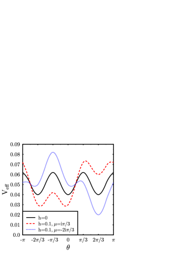
Figure 1: The effective potential ${\cal V}_{e\!f\!f}$ for the $SU(3)$ matrix model at imaginary $\mu$; there is no gluon loop potential. In all curves, $|\ell|=0.2$, with $\theta$ the phase of the loop: the solid curve is $h=0$, the dotted curve $h=0.1$ and $\mu=-2\pi i/3$, the dashed curve $h=0.1$ and ${\mu}=i\pi/3$.

As a check on our numerical analysis, we first discuss the case where $\mu$ is purely imaginary, $\mu=i\widetilde{\mu}$, which is a $U(1)$ rotation of the Wilson line:

$${\cal V}_{qk}({\bf L})=-\frac{h}{2}\left({\rm e}^{i\widetilde{\mu}}\;\ell_{3}\;+\;{\rm e}^{-i\widetilde{\mu}}\;\ell_{\overline{3}}\right)\;.$$ (30)

If the overall symmetry were $U(3)$, instead of $SU(3)$, then the Vandermonde potential is independent of $\widetilde{\mu}$. For a $SU(3)$ theory, however, the $Z(3)$ symmetry only requires that the potential is degenerate when $\widetilde{\mu}=0$ and $\pm 2\pi/3$.

As $\widetilde{\mu}$ represents an ordinary background field, the anti-triplet loop is the complex conjugate of the triplet loop. Defining $\theta$ as the phase of $\ell$, $\ell=\exp(i\theta)|\ell|$, then $\ell_{*}=\exp(-i\theta)|\ell|$, and the Vandermonde potential is a function of $|\ell|$ and $\theta$.

To illustrate the physics, in Fig. 1 we show three examples, with $h=0.0$ or $0.1$, and $|\ell|=0.2$. When there is no background field, $h=0$, there are three degenerate minima at $\theta=0$ and $\pm 2\pi/3$. When $h\neq 0$ and $\widetilde{\mu}=-2\pi/3$, the background field “tilts” the potential so that the expectation value is along the opposite direction, for $\theta=2\pi/3$. Lastly, when $h\neq 0$, and for the special choice of $\widetilde{\mu}=\pi/3$, the background field points exactly in the direction opposite to the minimum at $2\pi/3$; then there are two degenerate minima, for $\theta=0$ and $-2\pi/3$. The potential for other values of $\theta$ and $\ell$ follows similarly. Also, it is clear that, as a function of $\widetilde{\mu}$, the expectation value of $\theta$ is discontinuous at $\widetilde{\mu}=\pi/3$, jumping from 0 to $-2\pi/3$. Analytic continuation of ${\cal Z}$ to real $\mu$ is therefore possible only for $|\mu|<\pi/3$.

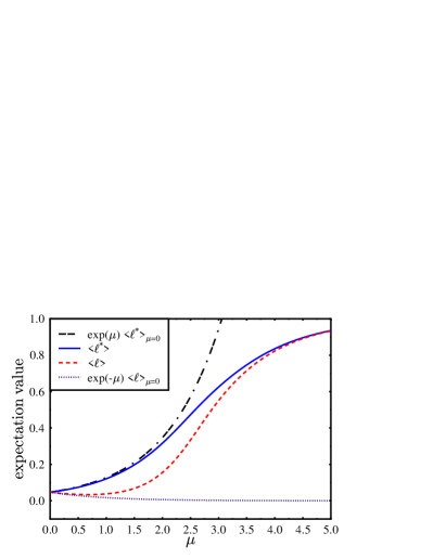
Figure 2: The expectation values $\langle\ell\rangle$ and $\langle\ell^{*}\rangle$ as functions of $\mu$ for $h=0.1$ and $m^{2}=0$.

When the chemical potential is real, as noted from (12) and (13), $\langle\ell\rangle$ and $\langle\ell^{*}\rangle$ are unequal but real. Fig. 2 shows the expectation values of the loop and of its conjugate for a background field $h=0.1$ (again without a gluon loop potential). For small $h$ and $\mu=0$, an analytical discussion of the $N=\infty$ potential at the Gross-Witten point shows that $\langle\ell\rangle\simeq h/2$, cf. section IIIB in dlp . From Fig. 2 one observes that this remains approximately true also for three colors.

At non-zero $\mu$ then, $\langle\ell\rangle$ and $\langle\ell^{*}\rangle$ split, which is due to the imaginary part of the fermion contribution (8) to the loop action. While $\langle\ell^{*}\rangle$ increases monotonically with $\mu$, $\langle\ell\rangle$ initially decreases from its value at $\mu=0$, cf. eq. (14). Finally, both expectation values approach one at large $\mu$, in accord with our discussion in Sec. I.

In Sec. II we saw that in a $U(1)$ model, the $\mu$-dependence of the expectation values is entirely given by a factor $\exp(\pm\mu)$, (19). We have checked numerically that this is approximately valid for $SU(3)$ when the chemical potential is very small. Fig. 2 shows, however, that this fails when $\mu\sim 1$.

In a matrix model, $\ell_{3}$ and $\ell_{\overline{3}}$ are traces of matrices. One could also consider a Polyakov loop model polyakov_loop , where $\ell_{3}$ and $\ell_{\overline{3}}$ are just scalar fields. To reduce the global symmetry from $U(1)$ to $Z(3)$, it is necessary to include cubic terms, such as $(\ell_{3})^{3}+(\ell_{\overline{3}})^{3}$, (3). As for the matrix model, one finds that the expectation values of $\ell_{3}$ and $\ell_{\overline{3}}$ differ when $\mu\neq 0$. Their exact form depends upon the details of the loop potential.

We now turn to a discussion of the effective potential ${\cal V}_{e\!f\!f}(\ell,\ell_{*})$, for real chemical potential. We also include the gluon loop potential from eq. (2). The solutions of the stationarity conditions

$$\frac{\partial{\cal V}_{e\!f\!f}(\ell,\ell_{*})}{\partial\ell}=\frac{\partial{\cal V}_{e\!f\!f}(\ell,\ell_{*})}{\partial\ell_{*}}=0~{},$$ (31)

determine the expectation values of the triplet and anti-triplet loops, $\langle\ell_{3}\rangle$ and $\langle\ell_{\overline{3}}\rangle$. Due to (26), these equations can be rewritten as

$$\omega(\ell^{0}_{*},\ell^{0}) = -\frac{\partial}{\partial\ell}\left[{\cal V}_{gl}(\ell,\ell_{*})+{\cal V}_{qk}(\ell,\ell_{*})\right]\Big{|}_{\ell=\ell^{0},\ell_{*}=\ell^{0}_{*}}$$ (32)

$$= m^{2}\ell_{*}^{0}+\frac{h}{2}\,e^{\mu}$$

$$\omega_{*}(\ell^{0}_{*},\ell^{0}) = -\frac{\partial}{\partial\ell_{*}}\left[{\cal V}_{gl}(\ell,\ell_{*})+{\cal V}_{qk}(\ell,\ell_{*})\right]\Big{|}_{\ell=\ell^{0},\ell_{*}=\ell^{0}_{*}}$$ (33)

$$= m^{2}\ell^{0}+\frac{h}{2}\,e^{-\mu}~{}.$$

These equations have to be solved simultaneously with (24). Note that at the stationary point both $\omega$ and $\omega_{*}$ are real. Also, these equations, unlike (12) and (13) above, make it obvious that the expectation values of the loops are not determined by cancellations of positive and negative contributions: (32) and (33) do not involve any oscillating functions.

To show the shape of the effective potential we fix $\ell-\ell_{*}$ to its expectation value given in eqs. (12,13) or in eqs. (32,33) above. We then study ${\cal V}_{e\!f\!f}$ as a function of the remaining degree of freedom, $\ell+\ell_{*}$.

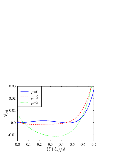
Figure 3: The effective potential at the peak of the Polyakov loop susceptibility for $h=10^{-3}$ and various $\mu$.

The behavior of the effective potential with nonzero $h$ and $\mu$ is customary of a first order transition in a background magnetic field. Fig. 3 shows the effective potential for $h=10^{-3}$ and $\mu=0$, 2, 3, respectively, as a function of $\ell+\ell_{*}$. For each curve, the coupling $m^{2}=m^{2}_{c}(\mu,h)$ is adjusted to maximize the susceptibility $\partial\langle\ell_{3}+\ell_{\overline{3}}\rangle/\partial m^{2}$. For such a weak background field, the first-order phase transition persists at $\mu=0$. As $\mu$ increases, the two minima of ${\cal V}_{e\!f\!f}$ approach each other and the barrier decreases. The first-order phase transition ends in a critical point at $\mu=\mu_{E}$. The transition is of second order at $\mu_{E}$, as the mass of the real part of the triplet loop vanishes. From Fig. 3, $\mu_{E}\approx 2.0$. As the chemical potential increases above $\mu_{E}$, the mass increases again, and there is no phase transition.

To date, Monte Carlo simulations have been performed for large $T$ and small $\mu$ fodor_katz ; swansea_bielefeld ; deforcrand_philipsen ; gavai_gupta . A matrix model predicts that $\langle\ell\rangle\neq\langle\ell^{*}\rangle$ when $\mu\neq 0$. The first work of Allton et al. swansea_bielefeld did not test this directly, but finds that $\langle\ell\rangle$ changes when the sign of $\mu$ is flipped. They did not plot $\langle\ell\rangle$ or $\langle\ell^{*}\rangle$ versus $\mu$, and so did not test the prediction that one of these expectation values is not monotonic in $\mu$.

The analysis of the present paper is most applicable for heavy quarks. At $\mu=0$, the lattice gives us an outline of the phase transition for three degenerate flavors of massive quarks. The deconfining transition only persists for relatively heavy quarks, $m>m_{qk}^{end}$ lattice_review_temp ; in DRR , this was estimated to disappear for a pseudo-scalar mass of $\approx 1.8$ GeV. There is no phase transition for intermediate quark masses, with a first order chiral transition appearing for light quark masses. In all cases at $\mu=0$, the rise in the Polyakov loop appears to coincide with the decrease in the chiral order parameter.

The case of heavy quarks at $\mu\neq 0$ is then similar to that of Fig. 3: a first order transition at $\mu=0$, ending in a critical end point at some $\mu_{E}$. (See, also, Fig. 1 of AKKS ). For quarks lighter than $m_{qk}^{end}$, there is no deconfining transition, and the correlation length of the Polyakov loop decreases monotonically as $\mu$ increases from zero. In the plane of $\mu$ and $T$, there may be a critical end point at $\mu\neq 0$, where the correlation length for the sigma meson diverges srs ; that for the Polyakov loop will remain finite, except from its coupling to the sigma.

To describe the region of small quark masses, and the chiral transition, it is necessary to introduce a chiral order parameter, and couple that to the Wilson line. A mean field approximation can be analyzed in a matrix model with two coupled matrices toappear . Due to the large $N$ argument mentioned at the end of Sec. II, it is possible that for three colors, the coincidence of the chiral and deconfining “transitions”, ubiquitous at $\mu=0$, breaks down at some finite value of $\mu$. That is, for intermediate quark densities, hadronic matter exists as a Fermi sea of “confined”, but chirally symmetric, nucleons.

IV Lattice QCD and the Fermion Sign Problem

We conclude by discussing how the results of the matrix model may be of use for numerical simulations of dense quarks in lattice QCD.

In Euclidean spacetime, the quark part of the action is

$${\cal S}_{qk}\;=\;\int d^{4}x\;\;\overline{\psi}\left(D\!\!\!\!/+\mu\gamma^{0}+m\right)\psi\;.$$ (34)

We follow the conventions of zinn_justin , with $D\!\!\!\!/=(\partial_{\mu}-igA_{\mu})\gamma^{\mu}$ the covariant derivative for a gluon field $A_{\mu}$. In this section, and in contrast to previous notation, here $\mu$ is the quark chemical potential (not $\mu/T$), and $m$ is the quark mass (not $m_{qk}$).

We need to use two symmetries. By a combination of Hermitian conjugation, plus a $\gamma_{5}$ transformation,

$$\left({\rm det}(D\!\!\!\!/+\mu\gamma^{0}+m)\right)^{*}\;=\;{\rm det}(D\!\!\!\!/-\mu\gamma^{0}+m)\;;$$ (35)

see, e.g., (13) of splittorff1 . At zero chemical potential, $D\!\!\!\!/$ is purely anti-Hermitian; as $D\!\!\!\!/$ anti-commutes with the matrix $\gamma_{5}$, the eigenvalues pair up, and the quark determinant is real. At nonzero chemical potential, the quark operator is a sum of an anti-Hermitian operator, $D\!\!\!\!/$, and a Hermitian operator, $\mu\gamma_{0}$. While the eigenvalues form pairs with opposite sign, (35) shows that the quark determinant is complex when $\mu\neq 0$. This is the fermion sign problem in dense QCD.

We can perform a charge conjugation transformation on the quarks zinn_justin . This is a change of variables in the Grassman integration over the quarks, and so it doesn’t change the determinant. This gives

$${\rm det}\left(D\!\!\!\!/+\mu\gamma^{0}+m\right)\;=\;{\rm det}\left(D\!\!\!\!/_{c}-\mu\gamma^{0}+m\right)\;,$$ (36)

where $D\!\!\!\!/_{c}=(\partial_{\mu}+igA_{\mu}^{*})\gamma^{\mu}$ is the covariant derivative for the charge conjugate gluon field, $-A_{\mu}^{*}$. By itself, this isn’t of much help, as we have changed the sign of the chemical potential, and turned the gluon field into its charge conjugate. In the matrix model, this symmetry is manifest in (5).

We now combine these two relations, to obtain:

$${\rm det}(D\!\!\!\!/_{c}+\mu\gamma^{0}+m)\;=\;\left({\rm det}(D\!\!\!\!/+\mu\gamma^{0}+m)\right)^{*}\;.$$ (37)

This shows that for the same sign of $\mu$, the quark determinant for charge conjugate gluons is the complex conjugate of the quark determinant in the original gluon field. This generalizes what is obvious in the matrix model.

Thus while the quark determinant in the presence of a given gluon field is complex, by adding the contribution of the charge conjugate gluons, we immediately obtain a partition function whose measure is manifestly real. This extends immediately to the lattice. There, gluons live on links, with link fields $U_{\mu}=\exp(igaA_{\mu})$, where “$a$” is the lattice spacing. A configuration of links is given by some set of $U_{\mu}$’s; the charge conjugate lattice is simply given by replacing each $U_{\mu}$ by $U_{\mu}^{*}$. That one can, in this way, obtain a real measure of the functional integral was known from the work of the Glasgow group (see, e.g., the discussion just before Eq. (8) in the last reference of glasgow ).

However, all this does is to reduce the problem from one of complex phases, to one of real phases. There are still configurations in the functional integral with both positive and negative weight. This still leaves the problem of how to decide whether to sum over configurations with both signs. Also, how does one include the effects of a Fermi sea of quarks in weighting configurations?

The matrix model provides clues to both of these questions. It is true that configurations of both signs contribute to the integral of the matrix model. However, at zero density, the background $Z(N)\;$field which quarks induce provides an expectation value along a definite direction in the complex plane, for real values (this is related to the sign of the quark masses). Further, at nonzero quark density, the field for the imaginary part of the loop has an imaginary coefficient, so that the expectation values of both $\ell$ and $\ell^{*}$ remain real and positive. We have checked that even at nonzero $\mu$, the dominant configurations of the matrix model are those in which the measure is positive.

It is reasonable to conjecture that this remains true with dynamical quarks. This suggests that in Monte Carlo simulations, that one accept configurations in which the quark determinant is positive, and drop those in which it is negative.

How, then, does one weight by configurations which include the effects of a Fermi sea of quarks? This could be included by a type of tadpole improvement. Suppose that one works out from zero chemical potential, to increasingly large values. To represent the effects of $\mu\neq 0$, one would expand not about the bare link variables, but about links equal to the expectation value of the loop. For a link going forward, one would use $\langle\ell\rangle$; for a link going backward, $\langle\ell^{*}\rangle$. This will explicitly bias one to configurations which include, approximately, the effects of the Fermi sea.

This is supported by numerical simulations of Blum, Hetrick, and Toussaint for heavy quarks blum . Using their results, de Forcrand and Laliena deforcrand_lal showed that the phase of the (heavy) quark determinant is proportional to the phase of the Polyakov loop, times the spatial volume.

These results illustrate a more general problem. The parameters of a matrix model are just numbers. This represents, however, a mean field approximation to the theory in a spatial volume, $V$. For example, the background field induced by quarks is itself proportional to $V$. For a measure which is always real and positive, this is of no concern: even if $h\sim V$, an error of order one is inessential relative to the dominant term, which is $\exp(-\#h)\sim\exp(-\#V)$. The integrals which enter at nonzero density, however, are those in which the measure includes oscillatory terms, as in (9), (12), and (13). In this case, it is necessary to determine the phase accurately not just to $\sim V$, but to $\sim 1$! In essence, this is the true fermion sign problem: not that the measure is not positive definite, but that one must determine the phase of the quark determinant very accurately. We note that similar oscillations in the quark determinant have been derived, using random matrix theory in the $\epsilon$-regime, by Osborn, Splittorff and Verbaarschot splittorff2 .

Nevertheless, we suggest that these techniques might be of use in numerical simulations of dense QCD on the lattice. By their nature, they are most suited for heavy quarks, starting from the region of zero density, and working out to nonzero density. Even if one accepts configurations whose overall weight is positive, it is certainly necessary to use cluster algorithms to include regions in which the phase is negative merons_etc .

We have used an effective model which is, implicitly, valid only for distances $\gg 1/T$. When the temperature is small, it is also imperative to include fluctuations in the expectation values of timelike links, as they wander about in (imaginary) time.

Lastly, these ideas are strongly motivated by the heavy quark limit blum ; deforcrand_lal , where quarks only propagate upward in imaginary time. Light quarks also propagate in space, so that at nonzero density, one will have to expand about modified expectation values for propagation which is “forward” or “backward” in proper time.

There is now a wealth of results available at nonzero temperature and small chemical potential fodor_katz ; swansea_bielefeld ; deforcrand_philipsen ; gavai_gupta ; splittorff1 ; splittorff2 . This is the first place to test our admittedly speculative remarks.

Acknowledgements: R.D.P. is supported by the U.S. Department of Energy grant DE-AC02-98CH10886, and thanks the Alexander von Humboldt Foundation for their support. He also thanks the following for discussions: T. Blum, M. Creutz, Dr. Flotte, K. Fukushima, T. Izubuchi, F. Karsch, S. Ohta, P. Petreczky, K. Splittorff, and most especially, D. H. Rischke.

References

- (1) E. Laermann and O. Philipsen, [arXiv:hep-ph/0303042]; F. Karsch and E. Laermann, [arXiv:hep-lat/0305025].
- (2) S. Muroya, A. Nakamura, C. Nonaka and T. Takaishi, Prog. Theor. Phys. 110, 615 (2003), [arXiv:hep-lat/0306031]; M. P. Lombardo, Prog. Theor. Phys. Suppl. 153, 26 (2004), [arXiv:hep-lat/0401021].
- (3) P. Hasenfratz and F. Karsch, Phys. Lett. B 125, 308 (1983).
- (4) F. Karsch and H. W. Wyld, Phys. Rev. Lett. 55, 2242 (1985).
- (5) P. E. Gibbs, Phys. Lett. B 182, 369 (1986).
- (6) A. Gocksch, Phys. Rev. Lett. 61, 2054 (1988); Phys. Rev. D 37, 1014 (1988).
- (7) I. M. Barbour and Z. A. Sabeur, Nucl. Phys. B 342, 269 (1990); I. M. Barbour and A. J. Bell, Nucl. Phys. B 372, 385 (1992); A. Hasenfratz and D. Toussaint, Nucl. Phys. B 371, 539 (1992); I. M. Barbour, A. J. Bell and E. G. Klepfish, Nucl. Phys. B 389, 285 (1993), [arXiv:hep-lat/9205019]; I. M. Barbour, S. E. Morrison, E. G. Klepfish, J. B. Kogut and M. P. Lombardo, Phys. Rev. D 56, 7063 (1997), [arXiv:hep-lat/9705038]; I. M. Barbour, S. E. Morrison, E. G. Klepfish, J. B. Kogut and M. P. Lombardo, Nucl. Phys. Proc. Suppl. 60A, 220 (1998), [arXiv:hep-lat/9705042].
- (8) M. A. Stephanov, Phys. Rev. Lett. 76, 4472 (1996), [arXiv:hep-lat/9604003].
- (9) M. G. Alford, A. Kapustin and F. Wilczek, Phys. Rev. D 59, 054502 (1999), [arXiv:hep-lat/9807039].
- (10) T. C. Blum, J. E. Hetrick and D. Toussaint, Phys. Rev. Lett. 76, 1019 (1996), [arXiv:hep-lat/9509002].
- (11) P. de Forcrand and V. Laliena, Phys. Rev. D 61, 034502 (2000), [arXiv:hep-lat/9907004].
- (12) K. Langfeld and G. Shin, Nucl. Phys. B 572, 266 (2000) [arXiv:hep-lat/9907006].
- (13) J. Condella and C. DeTar, Phys. Rev. D 61, 074023 (2000), [arXiv:hep-lat/9910028].
- (14) M. G. Alford, S. Chandrasekharan, J. Cox, and U.J. Wiese, Nucl. Phys. B 602, 61 (2001), [arXiv:hep-lat/0101012].
- (15) G. Aarts, O. Kaczmarek, F. Karsch and I. O. Stamatescu, Nucl. Phys. Proc. Suppl. 106, 456 (2002), [arXiv:hep-lat/0110145].
- (16) R. H. Swendsen and J. Wang, Phys. Rev. Lett. 58, 86 (1987); W. Bietenholz, A. Pochinsky and U. J. Wiese, Phys. Rev. Lett. 75, 4524 (1995), [arXiv:hep-lat/9505019]; S. Chandrasekharan and U.-J. Wiese, Phys. Rev. Lett. 83, 3116 (1999), [arXiv:cond-mat/9902128]; S. Chandrasekharan, J. Cox, K. Holland and U. J. Wiese, Nucl. Phys. B 576, 481 (2000), [arXiv:hep-lat/9906021]; J. Cox and K. Holland, Nucl. Phys. B 583, 331 (2000), [arXiv:hep-lat/0003022]; S. Chandrasekharan and J. C. Osborn, Phys. Lett. B 496, 122 (2000), [arXiv:hep-lat/0010036]; S. Chandrasekharan, J. Cox, J.C. Osborn, and U.J. Wiese, Nucl. Phys. B 673, 405 (2003), [arXiv:cond-mat/0201360]; S. Chandrasekharan, J. Cox, J.C. Osborn, and U.-J. Wiese, Nucl. Phys. B 673, 405 (2003), [arXiv:cond-mat/0201360]; B. B. Beard, M. Pepe, S. Riederer and U. J. Wiese, Phys. Rev. Lett. 94, 010603 (2005), [arXiv:hep-lat/0406040]; M Troyer and U.-J. Wiese, [arXiv:cond-mat/0408370].
- (17) K.N. Anagnostopoulos and J. Nishimura, Phys. Rev. D 66, 106008 (2002), [arXiv:hep-th/0108041]; J. Ambjorn, K.N. Anagnostopoulos, J. Nishimura, and J.J.M. Verbaarschot, Jour. of High Energy Phys. 0210, 062 (2002), [arXiv:hep-lat/0208025]; J. Ambjorn, K. N. Anagnostopoulos, J. Nishimura and J. J. M. Verbaarschot, Phys. Rev. D 70, 035010 (2004), [arXiv:hep-lat/0402031].
- (18) Z. Fodor and S. D. Katz, Phys. Lett. B 534, 87 (2002), [arXiv:hep-lat/0104001]; Jour. of High Energy Phys. 0203, 014 (2002), [arXiv:hep-lat/0106002]; Z. Fodor, S. D. Katz and K. K. Szabo, Phys. Lett. B 568, 73 (2003), [arXiv:hep-lat/0208078]; F. Csikor, G. I. Egri, Z. Fodor, S. D. Katz, K. K. Szabo and A. I. Toth, Jour. of High Energy Phys. 0405, 046 (2004), [arXiv:hep-lat/0401016]; Z. Fodor and S. D. Katz, Jour. of High Energy Phys. 0404, 050 (2004), [arXiv:hep-lat/0402006].
- (19) C. R. Allton et al., Phys. Rev. D 66, 074507 (2002) [arXiv:hep-lat/0204010]; ibid. 68, 014507 (2003), [arXiv:hep-lat/0305007]; ibid. 71, 054508 (2005), [arXiv:hep-lat/0501030]
- (20) A. Hart, M. Laine and O. Philipsen, Nucl. Phys. B 586, 443 (2000), [arXiv:hep-ph/0004060]; Phys. Lett. B 505, 141 (2001), [arXiv:hep-lat/0010008]; P. de Forcrand and O. Philipsen, Nucl. Phys. B 642, 290 (2002), [arXiv:hep-lat/0205016]; ibid. 673, 170 (2003), [arXiv:hep-lat/0307020].
- (21) R. V. Gavai and S. Gupta, Phys. Rev. D 68, 034506 (2003), [arXiv:hep-lat/0303013]; [arXiv:hep-lat/0412035].
- (22) G. Akemann, J. C. Osborn, K. Splittorff and J. J. M. Verbaarschot, Nucl. Phys. B 712, 287 (2005), [arXiv:hep-th/0411030].
- (23) J. C. Osborn, K. Splittorff and J. J. M. Verbaarschot, [arXiv:hep-th/0501210]; K. Splittorff, [arXiv:hep-lat/0505001].
- (24) G. ’t Hooft, Nucl. Phys. B 138, 1 (1978); ibid. 153, 141 (1979); A. M. Polyakov, Phys. Lett. B 72, 477 (1978); L. Susskind, Phys. Rev. D 20, 2610 (1979).
- (25) L. D. McLerran and B. Svetitsky, Phys. Rev. D 24, 450 (1981).
- (26) T. Banks and A. Ukawa, Nucl. Phys. B 225, 145 (1983).
- (27) S. I. Azakov, P. Salomonson and B. S. Skagerstam, Phys. Rev. D 36, 2137 (1987); D. E. Miller and K. Redlich, Phys. Rev. D 37, 3716 (1988).
- (28) R. D. Pisarski, Phys. Rev. D 62, 111501 (2000), [arXiv:hep-ph/0006205]; A. Dumitru and R. D. Pisarski, Phys. Lett. B 504, 282 (2001), [arXiv:hep-ph/0010083]; ibid. 525, 95 (2002), [arXiv:hep-ph/0106176]; Phys. Rev. D 66, 096003 (2002), [arXiv:hep-ph/0204223]; A. Dumitru, O. Scavenius, and A. D. Jackson, Phys. Rev. Lett. 87, 182302 (2001), [arXiv:hep-ph/0103219]; O. Scavenius, A. Dumitru and J. T. Lenaghan, Phys. Rev. C 66, 034903 (2002), [arXiv:hep-ph/0201079]; R. D. Pisarski, [arXiv:hep-ph/0203271].
- (29) A. Dumitru, D. Röder and J. Ruppert, [arXiv:hep-ph/0311119].
- (30) A. Mocsy, F. Sannino and K. Tuominen, Phys. Rev. Lett. 91, 092004 (2003) [arXiv:hep-ph/0301229]; Jour. of High Energy Phys. 0403, 044 (2004) [arXiv:hep-ph/0306069]; [arXiv:hep-ph/0308135]; F. Sannino and K. Tuominen, [arXiv:hep-ph/0403175].
- (31) K. Fukushima, Phys. Rev. D 68, 045004 (2003), [arXiv:hep-ph/0303225]; Phys. Lett. B 591, 277 (2004), [arXiv:hep-ph/0310121]; Y. Hatta and K. Fukushima, Phys. Rev. D 69, 097502 (2004), [arXiv:hep-ph/0307068].
- (32) A. Dumitru, Y. Hatta, J. Lenaghan, K. Orginos and R. D. Pisarski, Phys. Rev. D 70, 034511 (2004), [arXiv:hep-th/0311223].
- (33) A. Dumitru, J. Lenaghan and R. D. Pisarski, Phys. Rev. D 71, 074004 (2005), [arXiv:hep-ph/0410294].
- (34) O. Kaczmarek, F. Karsch, P. Petreczky, and F. Zantow, Phys. Lett. B 543, 41 (2002), [arXiv:hep-lat/0207002]; S. Digal, S. Fortunato and P. Petreczky, Phys. Rev. D 68, 034008 (2003), [arXiv:hep-lat/0304017]; O. Kaczmarek, F. Karsch, P. Petreczky and F. Zantow, Nucl. Phys. Proc. Suppl. B 129, 560 (2004), [arXiv:hep-lat/0309121]; P. Petreczky and K. Petrov, Phys. Rev. D 70, 054503 (2004), [arXiv:hep-lat/0405009]; O. Kaczmarek, F. Karsch, F. Zantow and P. Petreczky, Phys. Rev. D 70, 074505 (2004), [arXiv:hep-lat/0406036]
- (35) O. Aharony, J. Marsano, S. Minwalla, K. Papadodimas, and M. Van Raamsdonk, [arXiv:hep-th/0310285], v.5; [arXiv:hep-th/0502149].
- (36) H. J. Schnitzer, Nucl. Phys. B 695, 267 (2004), [arXiv:hep-th/0402219].
- (37) K. Furuuchi, E. Schreiberg, and G. Semenoff, [arXiv:hep-th/0310286]; O. Aharony, J. Marsano, S. Minwalla and T. Wiseman, Class. Quant. Grav. 21, 5169 (2004), [arXiv:hep-th/0406210]; H. Liu, [arXiv:hep-th/0408001]; M. Spradlin and A. Volovich, [arXiv:hep-th/0408178]; L. Alvarez-Gaume, C. Gomez, H. Liu and S. Wadia, [arXiv:hep-th/0502227].
- (38) M. Oswald and R. D. Pisarski, work in progress.
- (39) J. Zinn-Justin, “Quantum Field Theory and Critical Phenomena” (Clarendon Press, Oxford, 1997).
- (40) M. Stephanov, K. Rajagopal, and E. Shuryak, Phys. Rev. Lett. 81, 4816 (1998), [arXiv:hep-ph/9806219].
- (41) A. Dumitru, R. D. Pisarski, and D. Zschiesche, work in progress.