Oscillations of neutrinos produced and detected in crystals

Abstract

We analyze neutrino oscillations in a thought experiment in which neutrinos are produced by electrons on target nuclei. The neutrinos are detected through charged lepton production in their collision with nuclei in detector. Both the target and the detector are assumed to be crystals. The neutrinos are described by propagators. We find that different neutrino mass eigenstates have equal energies. We reproduce the standard phase of oscillations and demonstrate that at large distance from the production point oscillations disappear.

1 Introduction

Neutrino properties are of great interest for particle physics, astrophysics and cosmology. One of the main sources of information about neutrinos is an investigation of neutrino oscillations. Although a great many of papers on neutrino oscillations were published, there is still no common point of view on this phenomenon. One way to study neutrino oscillations is to consider neutrinos in the framework of the standard plane-wave description. Such an approach neglects effects which concern production and detection of neutrinos and demands choosing between two scenarios:
1) equal momentum scenario (see papers by Gribov and Pontecorvo [1] and by Fritzsch and Minkovski [2]),
2) equal energy scenario (see papers by Lipkin [3] and Stodolsky [4] as well as by Kobzarev et al. [5] and Grimus and Stockinger [6]). In ref.[6] neutrino was created in $\beta$-decay of a neutron localized at point $P$ and detected through its interaction with an electron localized at point $D$. In refs.[5] and [7] the authors considered neutrino produced by an electron beam on the target nucleus $A$ and detected through its interaction with the nucleus $B$ of the detector. The whole process looked as (see Fig. 1)

$$e+A+B\rightarrow l+C+D,$$ (1)

where $l$ is a lepton ($e$, $\mu$ or $\tau$), while $C$ and $D$ are recoil nuclei. In ref. [7] the nuclei $A$ and $B$ were supposed to be unconfined in a gaseous target/detector and described by wave packets; the electron wave function was also assumed to be a wave packet.

In this article we investigate a thought experiment similar to that considered in ref. [7] but with nuclei $A$ and $B$ bound in crystals. We use the rigorous quantum field theory approach (Feynman diagram with neutrino propagators) to achieve the following goals:
1) to show that in the case under consideration equal energy scenario takes place,
2) to reproduce the standard form of the oscillation phase,
3) to integrate over the phase space of the final particles in order to obtain the probability of the process,
4) to demonstrate that oscillations disappear at large distances from the production point,
5) to investigate corrections due to non-zero temperature and to show that they are not essential for the range of temperatures at which crystals may exist.

One of the reasons to write this paper is that in the year 2004 in the most authoritative particle physics review of Particle Data Group the so-called ”equal momentum scenario” was chosen to describe neutrino oscillations [8]. We think, following Vysotsky [9], that though this approach gives the standard result, it is not self-consistent and thus misleading: neutrinos produced at point $A$ (by electron) would not have a definite (electronic) flavor, but their flavor would oscillate with time at point $A$.

In the case of solid state detector with stationary nuclei the neutrino energy is determined by energy conservation for the interaction in the detector and does not depend on neutrino masses. This conforms with the point of view of Lipkin [3]. Contrary to that the momentum cannot have a certain value because of the uncertainty relation for spatially localized nuclei.

The paper is organized as follows. In section 2 we derive the amplitude for the process (1) and obtain the oscillation phase. In section 3 we integrate modulus of the amplitude squared over the momenta of the final nuclei and over the energy of the final lepton. In sections 2 and 3 the temperature is supposed to be zero. In section 4 the case of non-zero temperature is considered. Our main results are summarized in section 5. Appendix contains derivation of factors which suppress oscillations at large distances.

2 Nuclei bound in crystals at zero temperature

In this section we follow the lines (and the notations) of ref.[7]. The difference is in the initial wave functions of the target and detector nuclei: they are stationary in this article while in ref.[7] they were represented by wave packets.

Consider neutrino production by electron $e$ on a target nucleus $A$ of mass $M_{A}$. Then the neutrino collides with nucleus $B$ of mass $M_{B}$ in a detector and produces charged lepton $l$ (see Fig. 1) .

The electron neutrino $\nu_{e}$ produced on nucleus $A$ is a superposition of three neutrino mass eigenstates: $\nu_{e}=\sum_{j}U_{ej}\nu_{j}$, where $\nu_{j}$ is a state with mass $m_{j}$,  $U$ is a unitary mixing matrix, the first and second indices of which denote flavor and mass eigenstates, respectively. The detection of the neutrino by means of its interaction with $B$ results in the projection of three propagating neutrino states onto the final flavour state $\nu_{l}=\sum_{j}U_{lj}\nu_{j}$.

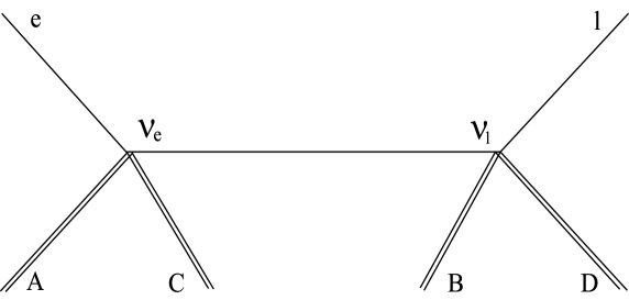
Figure 1: Little donkey diagram from ref. [7]

The amplitude of the process (1) is given by the following equation:

$$\mathcal{A}_{e\rightarrow l}=\sum_{j}U_{ej}^{*}U_{lj}\mathcal{A}_{j},$$ (2)

where $A_{j}$ is the amplitude for a given neutrino state of mass $m_{j}$ :

$$\mathcal{A}_{j}=\int d^{4}x_{2}d^{4}x_{1}\Psi_{B}(x_{2})\Psi^{*}_{l}(x_{2})\Psi_{D}^{*}(x_{2})G_{j}(x_{2}-x_{1})\Psi_{A}(x_{1})\Psi_{e}(x_{1})\Psi_{C}^{*}(x_{1})\leavevmode\nobreak\ .$$ (3)

Here $\Psi_{a}$ are wave functions of particles $a$; $G_{j}$ is the Green function of $j$-th mass eigenstate of neutrino, and $x_{k}=(t_{k},{\bf x}_{k})$ are 4-dimensional coordinates.

There exists a vast literature in which not only incoming but also outgoing particles are described by wave packets (see review by Beuthe [10]). We describe the electron by a wave packet, the initial nuclei $A$ and $B$ – by stationary wave functions, while the outgoing particles – by plane waves as representatives of a complete set of orthogonal states.

We assume that the initial nuclei $A$ and $B$ are bound in crystals and their wave functions are energy eigenstates localized near central point ${\bf x}_{A}$ and ${\bf x}_{B}$, respectively, with the uncertainty of the order of crystal spacing $a_{A,B}$. Their wave functions are taken as a product:

$$\Psi_{a}(x)=\psi_{a}({\bf x}-{\bf x}_{a})\leavevmode\nobreak\ e^{-itE_{a}}\leavevmode\nobreak\ ,$$ (4)

where $a=A,B$ and $E_{a}$ is the energy of nucleus in the potential of a crystal cell, which is equal to the difference of $M_{a}$ and binding energy. The Fourier transform of $\psi_{a}({\bf x})$, which we need in what follows, is

$$K_{a}({\bf q}_{a})=\int d{\bf x}\psi_{a}({\bf x}-{\bf x}_{a})e^{-i{\bf q}_{a}({\bf x}-\mathbf{x}_{a})}$$ (5)

By assumption, nuclei $A$ and $B$ are at rest and thus $K({\bf q}_{a})$ is centered near ${\bf q}_{a}=0$ with uncertainty $\sigma_{a}\sim a_{a}^{-1}$.

The wave function of the incident electron is taken as a wave packet:

$$\Psi_{e}(x)=\int d{\bf q}_{e}K_{e}({\bf q}_{e}-{\bf p}_{e})e^{i{\bf q}_{e}({\bf x}-{\bf x}_{e})-iE_{e}t},$$ (6)

where $E_{e}({\bf q}_{e})=\sqrt{{\bf q}_{e}^{2}+m_{e}^{2}}$, the Fourier amplitude $K_{e}({\bf q}_{e}-{\bf p}_{e})$ is centered near ${\bf q}_{e}={\bf p}_{e}$ with uncertainty $\sigma_{e}$, and the maximum of the envelope of the packet is at the point ${\bf x}_{e}$ at the moment $t=0$.

According to the measurements of Novosibirsk group (Pinaev et al., [11],[12]), which used an undulator at electron storage ring, $\sigma_{e}>0.7\times 10^{-6}$ eV = (30 cm)^-1. The theoretical analysis of this data and the mechanism of reduction of the wave packet of a relativistic charged particle by emission of a photon has been performed by Faleev [13]. (For the general theory of wave packets see lectures by Glauber [14].) As for the upper bound on $\sigma_{e}$, it is smaller then $10^{-3}E_{e}$ for an electron accelerator according to the PDG ([15], pp.239-241).

For the wave functions of the outgoing particles we can take any complete and orthogonal set of functions, the most convenient would be just plane waves:

$$\Psi_{c}^{*}(x)=e^{itE_{c}-i{\bf p}_{c}{\bf x}},$$ (7)

where $c=C,D,l$.

It is clear that fermionic nature of neutrino (as well as of $e$ and $l$) is not essential in the problem at high enough energies, therefore we replace the neutrino Green function by the Green function of a scalar particle of mass $m_{j}$, where $j$ enumerates neutrino mass eigenstates, $j=1,2,3$. Thus:

$$G_{j}(\mathbf{x},t)=\frac{1}{(2\pi)^{4}}\int\frac{e^{-i\omega t+i\mathbf{k}\mathbf{x}}}{\omega^{2}-\mathbf{k}^{2}-m^{2}_{j}+i\varepsilon}d\mathbf{k}d\omega\leavevmode\nobreak\ .$$ (8)

We integrate in (3) over $(t_{1}+t_{2})$ and $(t_{2}-t_{1})$ using

$$\int e^{i\omega(t_{2}-t_{1})}G_{j}(\mathbf{x}_{2}-\mathbf{x}_{1},t_{2}-t_{1})d(t_{2}-t_{1})=-\frac{1}{4\pi|\mathbf{x}_{1}-\mathbf{x}_{2}|}e^{i\sqrt{\omega^{2}-m_{j}^{2}}|\mathbf{x}_{1}-\mathbf{x}_{2}|}$$ (9)

and obtain

$$\mathcal{A}_{j}=-\int d\mathbf{x}_{1}d\mathbf{x}_{2}d\mathbf{q}_{e}K_{e}(\mathbf{q}_{e}-\mathbf{p}_{e})e^{i\mathbf{q}_{e}(\mathbf{x}_{1}-\mathbf{x}_{e})}\psi_{A}(\mathbf{x}_{1}-\mathbf{x}_{A})\psi_{B}(\mathbf{x}_{2}-\mathbf{x}_{B})$$

$$e^{-i\mathbf{p}_{C}\mathbf{x}_{1}-i\mathbf{p}_{D}\mathbf{x}_{2}-i\mathbf{p}_{l}\mathbf{x}_{2}}\leavevmode\nobreak\ \frac{e^{ik_{j}|\mathbf{x}_{1}-\mathbf{x}_{2}|}}{4\pi|\mathbf{x}_{1}-\mathbf{x}_{2}|}\leavevmode\nobreak\ \delta(E_{e}(\mathbf{q}_{e})+E_{A}-E_{C}-\omega)\leavevmode\nobreak\ ,$$ (10)

where

$$\omega\equiv E_{l}+E_{D}-E_{B}$$ (11)

and $\leavevmode\nobreak\ k_{j}\equiv\sqrt{\omega^{2}-m_{j}^{2}}.$ The delta-function in eq.(10) corresponding to the energy conservation for the whole process appears due to integration over $(t_{1}+t_{2})$.

We would like to emphasize that the energy $\omega$ of the virtual neutrino does not depend on $j$. The energy $\omega$ is determined by energy conservation at point $B$. Due to stationarity of nuclei $B,D$ and lepton $l$ (see eqs.(4) and (7)) the energy $\omega$ is the same for all neutrino mass eigenstates.

Note that $e^{ik_{j}|\mathbf{x}_{1}-\mathbf{x}_{2}|}$ is the only factor in eq.(10) which depends on $j$ and leads to mass-dependent effects such as oscillations. Since the initial nuclei $A$ and $B$ are in the potential wells, they are well localized near the points $\mathbf{x}_{A}$ and $\mathbf{x}_{B}$, respectively; therefore the integrand in eq.(10) is essentially different from zero if $|\mathbf{x}_{1}-\mathbf{x}_{A}|\lesssim a_{A}$ and $|\mathbf{x}_{2}-\mathbf{x}_{B}|\lesssim a_{B}$. Hence the effective range of integration over $\mathbf{x}_{1}$ and $\mathbf{x}_{2}$ is limited by $\left||\mathbf{x}_{1}-\mathbf{x}_{2}|-|\mathbf{x}_{A}-\mathbf{x}_{B}|\right|\lesssim a$, where $a_{A}\sim a_{B}\sim a$. Furthermore, $k_{j}$ differs slightly from $\omega$, so we may expand

$$k_{j}=\omega-\frac{m_{j}^{2}}{2\omega}+...$$ (12)

In what follows we introduce the following notation:

$$x_{AB}\equiv|\mathbf{x}_{A}-\mathbf{x}_{B}|\leavevmode\nobreak\ .$$ (13)

Then

$$e^{ik_{j}|\mathbf{x}_{1}-\mathbf{x}_{2}|}=e^{ik_{j}x_{AB}}\exp{\left[i\left(\omega+O\left(\frac{m_{j}^{2}}{2\omega}\right)\right)(|\mathbf{x}_{1}-\mathbf{x}_{2}|-x_{AB})\right]}=$$

$$=e^{ik_{j}x_{AB}}e^{i\omega(|\mathbf{x}_{1}-\mathbf{x}_{2}|-x_{AB})}\left[1+O\left(\frac{m_{j}^{2}}{2\omega}a\right)\right]\leavevmode\nobreak\ .$$ (14)

Lattice spacing $a$ is of order of $10^{-8}$ cm. As for the $\omega$ (which is roughly equal to the electron energy), it can vary depending on the beam energy of the accelerator which produces electrons. Let us take, for example,$\leavevmode\nobreak\ \omega=1$ GeV. This energy is sufficient for muons to be created in the detector. If we take $3$ eV as the upper bound for neutrino mass we get $am_{j}^{2}/(2\omega)<10^{-12}$, hence the $j$-dependent correction in brackets in eq.(14) can be neglected, and we obtain from eqs.(10) and (14):

$$\mathcal{A}_{j}=-e^{ik_{j}x_{AB}}\int d\mathbf{x}_{1}d\mathbf{x}_{2}d\mathbf{q}_{e}K_{e}(\mathbf{q}_{e}-\mathbf{p}_{e})e^{i\mathbf{q}_{e}(\mathbf{x}_{1}-\mathbf{x}_{e})}e^{-i\mathbf{p}_{C}\mathbf{x}_{1}-i\mathbf{p}_{D}\mathbf{x}_{2}-i\mathbf{p}_{l}\mathbf{x}_{2}}$$

$$\psi_{A}(\mathbf{x}_{1}-\mathbf{x}_{A})\psi_{B}(\mathbf{x}_{2}-\mathbf{x}_{B})\frac{e^{i\omega(|\mathbf{x}_{1}-\mathbf{x}_{2}|-x_{AB})}}{4\pi|\mathbf{x}_{1}-\mathbf{x}_{2}|}\delta(E_{e}(\mathbf{q}_{e})+E_{A}-E_{C}-\omega)\leavevmode\nobreak\ ,$$ (15)

We see that $e^{ik_{j}x_{AB}}$ is the only $j$-dependent factor in eq.(15), which means that the phase difference between $\mathcal{A}_{i}$ and $\mathcal{A}_{j}$ has the following form :

$$\phi_{ij}\equiv\phi_{i}-\phi_{j}=(k_{i}-k_{j})x_{AB}.$$ (16)

There is no term, containing energy difference, in the right-hand side of eq.(16). This results from equality of energies of different neutrino mass eigenstates, emphasized earlier. The form of the phase in eq.(16) allows to resolve the problem ”equal energy vs equal momentum” in favor of equal energy scenario.

From eqs.(12) and (16) we obtain the standard expression:

$$\phi_{ij}=-\frac{\delta m_{ij}^{2}}{2\omega}x_{AB},$$ (17)

where $\leavevmode\nobreak\ \delta m_{ij}^{2}\equiv m_{i}^{2}-m_{j}^{2}$.

To integrate over $\mathbf{x}_{1}$ and $\mathbf{x}_{2}$ in eq.(15) we take into account that $a_{A},a_{B}\ll x_{AB}$, and hence we can use the expansion

$$|\bf{x}\mit_{1}-\bf{x}\mit_{2}|\simeq x_{AB}-\bf{n}(\mathbf{x}_{1}-\mathbf{x}_{A})+\bf{n}(\mathbf{x}_{2}-\mathbf{x}_{B})\leavevmode\nobreak\ ,$$ (18)

where

$$\mathbf{n}=\frac{\mathbf{x}_{B}-\mathbf{x}_{A}}{x_{AB}}\leavevmode\nobreak\ .$$ (19)

From eqs.(18) and (15) we obtain (up to a constant phase factor):

$$A_{j}=\frac{e^{ik_{j}x_{AB}}}{x_{AB}}\,\int d{\bf q}_{e}e^{i\mathbf{q}_{e}(\mathbf{x}_{A}-\mathbf{x}_{e})}K_{e}({\bf q}_{e}-{\bf p}_{e})K_{A}({\bf q}_{A})K_{B}({\bf q}_{B})\delta\left(E_{in}-E_{fin}\right)$$ (20)

where

$$E_{in}=E_{A}+E_{B}+E_{e}\leavevmode\nobreak\ ,\leavevmode\nobreak\ \leavevmode\nobreak\$$

$$E_{fin}=E_{C}+E_{D}+E_{l}\leavevmode\nobreak\ ,$$

$${\bf q}_{A}={\bf p}_{C}+\omega\mathbf{n}-{\bf q}_{e}\leavevmode\nobreak\ ,$$

$${\bf q}_{B}={\bf p}_{l}+{\bf p}_{D}-\omega\mathbf{n}\leavevmode\nobreak\ .$$

As follows from eq.(20) and the expressions for the wave functions presented above, the amplitude is a function of the vector $\mathbf{n}$, neutrino mass, $m_{j}$, energies of the initial nuclei, $E_{A}$ and $E_{B}$, central momentum of the incoming electron ${\bf p}_{e}$, and momenta of the final particles ${\bf p}_{C},\leavevmode\nobreak\ \mathbf{p}_{D},\leavevmode\nobreak\ \mathbf{p}_{l}$.

In the next section we will use an explicit formula for the amplitude $A_{j}$ (eq.(20)) in the case of certain simple expressions for the crystal potential and for the wave packet of the electron. We assume that the electron is described by one-dimensional Gaussian wave packet with definite direction $\mathbf{e}=\mathbf{p}_{e}/|\mathbf{p}_{e}|$, that is

$$d\mathbf{q}_{e}=\delta\left(\frac{\mathbf{q}_{e}}{|\mathbf{q}_{e}|}-\mathbf{e}\right)\leavevmode\nobreak\ |\mathbf{q}_{e}|^{2}\leavevmode\nobreak\ d|\mathbf{q}_{e}|\leavevmode\nobreak\ d\Omega_{e}$$ (21)

$$K_{e}(\mathbf{q}_{e}-\mathbf{p}_{e})=\exp\left[-\frac{(\mathbf{q}_{e}-\mathbf{p}_{e})^{2}}{2\sigma_{e}^{2}}\right].$$ (22)

We also assume that the potential is an oscillator near the center of the crystal cell and a constant at large distances from this point. Furthermore we consider the initial nuclei in the ground states in their crystal cells:

$$K_{a}(\mathbf{q}_{a})=\exp\left({-\frac{\mathbf{q}_{a}^{2}}{2\sigma_{a}^{2}}}\right),$$ (23)

where $a=A,B.$ After integration over $\mathbf{q}_{e}$ in eq.(20) by using delta-function in the integrand of eq.(20) and delta-function in eq.(21) we obtain

$$A_{j}=E_{e}^{0}q_{e}^{0}\leavevmode\nobreak\ \frac{e^{ik_{j}x_{AB}}}{4\pi x_{AB}}\leavevmode\nobreak\ e^{i\mathbf{q}^{0}_{e}(\mathbf{x}_{A}-\mathbf{x}_{e})}$$

$$\exp\left[{-\frac{(q_{e}^{0}\bf{e}\mit-\bf{p}\mit_{e})^{2}}{2\sigma_{e}^{2}}}\right]\exp\left[{-\frac{(\omega\bf{n}\mit+\bf{p}\mit_{C}-q_{e}^{0}\bf{e}\mit)^{2}}{2\sigma_{A}^{2}}}\right]\exp\left[{-\frac{(\bf{p}\mit_{l}+\bf{p}\mit_{D}-\omega\bf{n}\mit)^{2}}{2\sigma_{B}^{2}}}\right],$$ (24)

where

$$E_{e}^{0}=E_{l}+E_{C}+E_{D}-E_{A}-E_{B},$$ (25)

and

$$q_{e}^{0}=\sqrt{(E^{0}_{e})^{2}-m_{e}^{2}}.$$ (26)

Thus introduced $q_{e}^{0}$ coincides with $p_{e}=|{\bf p}_{e}|$ within $\sigma_{e}$.

3 Integration over phase space

In this section we integrate the probability of the process (1) over the phase volume of the final nuclei and over the energy of the final lepton, assuming explicit form of the crystal potential and of the electron wave packet (see the end of the previous section). We demonstrate that due to the neutrino energy dispersion the oscillations are suppressed at large distances. We think that this result is valid for arbitrary shapes of wave packets.

We consider a situation when only the direction of the final lepton is measured, while its energy is not measured and final nuclei are not registered . Thus we are interested in the differential probability for the final lepton to be detected in the solid angle $d\Omega_{l}$ :

$$\frac{dP_{e\rightarrow l}}{d\Omega_{l}}\equiv\int|\mathcal{A}_{e\rightarrow l}|^{2}\frac{d\mathbf{p}_{C}}{2E_{C}}\frac{d\mathbf{p}_{D}}{2E_{D}}\frac{p^{2}_{l}dp_{l}}{2E_{l}}=\sum_{ij}U_{ej}^{*}U_{lj}U_{ei}U^{*}_{li}{\cal P}_{ij}.$$ (27)

Here $p_{l}\equiv|\mathbf{p}_{l}|$; $\leavevmode\nobreak\ \mathbf{p}_{C}$, $\mathbf{p}_{D}$ and $\mathbf{p}_{l}$ are the momenta of the final nuclei and the final lepton, correspondingly, and

$${\cal P}_{ij}\equiv\int P_{ij}\frac{d\mathbf{p}_{C}}{2E_{C}}\frac{d\mathbf{p}_{D}}{2E_{D}}\frac{p^{2}_{l}dp_{l}}{2E_{l}},$$ (28)

where

$$P_{ij}\equiv\mathcal{A}_{i}^{*}\mathcal{A}_{j}.$$ (29)

We interpret the electron detection as $\nu_{e}$ survival, and $\mu$ or $\tau$ detection as $\nu_{\mu}$ or $\nu_{\tau}$ appearance, respectively.

From eq.(24) we get:

$$P_{ij}=\frac{\exp\left(i\frac{\delta m_{ij}^{2}}{2\omega}x_{AB}\right)}{x_{AB}^{2}}\exp{\left[-\frac{(q_{e}^{0}{\bf e}-{\bf p}_{e})^{2}}{\sigma_{e}^{2}}-\frac{(\omega\bf{n}\mit+\bf{p}\mit_{C}-q_{e}^{0}\bf{e}\mit)^{2}}{\sigma_{A}^{2}}-\frac{(\bf{p}\mit_{l}+\bf{p}\mit_{D}-\omega\bf{n}\mit)^{2}}{\sigma_{B}^{2}}\right]}.$$ (30)

Here we delete inessential factors $1/(4\pi)^{2}$ and $(E_{e}^{0}q_{e}^{0})^{2}$. In what follows to simplify formulas we take

$M_{C}=M_{D}\equiv M\sim 100$ GeV, $\sigma_{A}=\sigma_{B}\equiv\sigma\sim 1$ keV; 10 MeV $\lesssim E_{e}\lesssim 1$ GeV.

For such choice of parameters the electron is relativistic, while

$$\frac{p_{e}}{M}\ll 1,$$ (31)

where $p_{e}\equiv|\mathbf{p}_{e}|$.

We calculate $\mathcal{P}_{ij}$, defined by eq.(28), in the Appendix for two cases:
1. Large $\sigma_{e}$:

$$\sigma_{e}\gg\sigma\frac{p_{e}}{M},$$ (32)

2. Small $\sigma_{e}$:

$$\sigma_{e}\ll\sigma\frac{p_{e}}{M}.$$ (33)

We assume that vectors $\mathbf{e}$ and $\mathbf{n}$ have a substantially nonzero angle between them and the module of their difference is of order of unity. We present the results in the form

$${\cal P}_{ij}\sim\exp\left(i\frac{x_{AB}}{L^{osc}_{ij}}\right)\exp\left[-\left(\frac{x_{AB}}{L^{sup}_{ij}}\right)^{2}\right]\leavevmode\nobreak\ ,$$ (34)

where $L^{osc}_{ij}\equiv 2E_{\nu}/\delta m^{2}_{ij}$, and, in our case, $E_{\nu}=p_{e}(1+O\left(\frac{p_{e}}{M}\right))$. For the first case (32)

$$L^{sup}_{ij}=L^{osc}_{ij}\frac{2p_{e}}{\sigma_{e}}\leavevmode\nobreak\ ,$$ (35)

(see eq.(A.30)), while for the second case (33)

$$L^{sup}_{ij}\sim L^{osc}_{ij}\frac{M}{\sigma},$$ (36)

(see eq.(A.41)).

The origin of the above suppression is neutrino energy dispersion, on which the oscillation length depends. A rather lengthy way to derive eqs.(34)-(36) is given in the Appendix.

A simple qualitative estimate of the suppression, based on consideration of two particle reaction $e+A\rightarrow\nu+C$, will be presented in ref.[16].

It is interesting to note that the suppression length for large $\sigma_{e}$ (the first case) is equal to that which arises due to spatial separation of the neutrino wave packets with different $m_{j}$, and hence different velocities, in the case when neutrinos are described not by a propagator, but by a wave function (see Dolgov et al. [16], Nussinov [17], Kayser [18] and Dolgov [19]).

As for the case of vanishingly small $\sigma_{e}$, there is no separation of neutrino wave packets considered in refs.[16]-[19], but suppression exists due to virtual neutrino energy dispersion.

Let us end up this section by considering a toy model of two neutrino flavours ($\nu_{e}$ and $\nu_{\mu}$, for definiteness). In this case from eqs.(27) and (34) we easily find

$$\frac{dP_{e\rightarrow e}}{d\Omega_{e}}=\left\{1-\frac{1}{2}(\sin 2\theta)^{2}\left[1-\exp{\left(-\frac{x^{2}_{AB}}{L^{2}_{sup}}\right)}\cos\left(\frac{x_{AB}}{L_{osc}}\right)\right]\right\}W(\mathbf{l}),\leavevmode\nobreak\$$

$$\frac{dP_{e\rightarrow\mu}}{d\Omega_{\mu}}=\frac{1}{2}(\sin 2\theta)^{2}\left[1-\exp{\left(-\frac{x^{2}_{AB}}{L^{2}_{sup}}\right)}\cos\left(\frac{x_{AB}}{L_{osc}}\right)\right]W(\mathbf{l})\leavevmode\nobreak\ ,$$ (37)

where $\mathbf{l}\equiv\frac{\mathbf{p}_{l}}{p_{l}},\leavevmode\nobreak\ U_{e1}=\cos\theta,\leavevmode\nobreak\ U_{e2}=\sin\theta$ and the factor $W(\mathbf{l})$ does not depend on the lepton flavour $l$ in the limit of ultra-relativistic final leptons.

4 Nuclei bound in crystals at non-zero
temperature

Now we show that for a non-zero temperature the results do not essentially change. In this case we cannot assume nuclei wave functions in crystal cells to be stationary. A general expression for the wave functions of the initial nuclei is the following:

$$\Psi_{A,B}(\mathbf{x},t)=\sum_{n}C_{A,B}^{n}\psi_{A,B}^{n}(\mathbf{x})\leavevmode\nobreak\ e^{-iE_{A,B}^{n}t},$$ (38)

where $n$ enumerates the states with definite energies $E_{A,B}^{n}$, while $C_{A,B}^{n}$ is the amplitude of probability to measure energy $E_{A,B}^{n}$ in the state with wave function $\Psi_{A,B}(\mathbf{x},t)$. Using the linearity of amplitudes with respect to initial wave functions we obtain

$$P_{ij}=\sum_{m}\sum_{m^{\prime}}C_{m}C^{*}_{m^{\prime}}\mathcal{A}^{*}_{i\leavevmode\nobreak\ m^{\prime}}\mathcal{A}_{j\leavevmode\nobreak\ m},$$ (39)

where for convenience we define the two-dimensional index $m\equiv(n_{1},n_{2})$, $C_{m}\equiv C_{A}^{n_{1}}C_{B}^{n_{2}}$, and $\mathcal{A}_{i\leavevmode\nobreak\ m}$ stands for $\mathcal{A}_{i}$ calculated with $\psi_{A}^{n_{1}}$ and $\psi_{B}^{n_{2}}$. For typographical reasons there is no difference between upper and lower indices.

Since we consider the case of a thermal equilibrium, we have to average $P_{ij}$ using $\overline{C_{m}C^{*}_{m^{\prime}}}=\delta_{mm^{\prime}}e^{-E_{m}/T}$, where $E_{m}\equiv E_{A}^{n_{1}}+E_{B}^{n_{2}}$. After averaging we obtain

$$\overline{P_{ij}}=\sum_{m}e^{-\frac{E_{m}}{T}}\mathcal{A}^{*}_{i\leavevmode\nobreak\ m}\mathcal{A}_{j\leavevmode\nobreak\ m}.$$ (40)

We see that taking temperature into account results in a simple averaging of $P_{ij}$ over different stationary initial states weighted with $e^{-E_{m}/T}$, which is a common case in statistical mechanics. Such a correction does not result in any observable effect due to the smallness of thermal energy $T$ compared with $\omega$. Indeed,

$$\phi_{ij}=-\frac{\delta m^{2}_{ij}}{2\omega}x_{AB}+O\left(\frac{\delta m^{2}_{ij}}{2\omega}\frac{T}{\omega}x_{AB}\right),$$ (41)

where $\omega$ corresponds to the case of zero temperature (ground states, $n_{2}=0$):

$$\omega=E_{l}+E_{D}-E_{B}^{0}.$$ (42)

We see that the correction is essential if $x_{AB}\sim\ (\omega/T)L_{osc}\sim 10^{10}\leavevmode\nobreak\ L_{osc}\leavevmode\nobreak\$ for $\omega=1$ GeV, $T=300$ K. In the previous section it was shown that at such distances oscillations are washed out. Thus we may safely neglect this correction and recover to the standard expression (17).

5 Conclusions

1.Our calculations explicitly confirm the equal energy scenario, advocated by Lipkin and Stodolsky (see text after eqs.(11) and (16)).
2.The oscillation phase has its standard form, see eq.(17).
3. When integrated over the phase volume of the final nuclei and over the energy of the final lepton, the oscillating term in the probability of the process under consideration vanishes exponentially at the distances $L_{sup}=(2p_{e}/\sigma_{e})L_{osc}$ for large $\sigma_{e}$, and $L_{sup}\sim(M/\sigma)L^{osc}_{ij}$ for small $\sigma_{e}$ including plane wave limit for electron; see eqs.(35) and (36).
4. For non-vanishing temperature $T$ the standard expression for the phase difference is valid up to correction $\sim(T/\omega)$.

6 Acknowledgments

We are grateful to A. Bondar, M. Danilov, K. Ter-Martirosyan, V. Vinokurov, and M. Vysotsky for fruitful discussions and interest to this work.

7 Appendix A

1. General formulas

The aim of this Appendix is to integrate $P_{ij}$ given by eq.(30) over the phase space of nuclei $C$ and $D$ and over the energy of the final lepton $l$:

$${\cal P}_{ij}=\int P_{ij}\frac{d\mathbf{p}_{C}}{2E_{C}}\frac{d\mathbf{p}_{D}}{2E_{D}}\frac{p_{l}dE_{l}}{2}.$$ (A.1)

In what follows for simplicity we consider an ultra-relativistic electron:

$$q^{0}_{e}=E^{0}_{e},$$ (A.2)

where $E_{e}^{0}$ and $q_{e}^{0}$ are defined by eqs.(25) and (26). We assume that the target and the detector contain the same nuclei:

$$M_{A}=M_{B}=M_{C}=M_{D}=M,\leavevmode\nobreak\ \sigma_{A}=\sigma_{B}=\sigma.$$ (A.3)

The Appendix consists of six parts. In part 1 (eqs.(A.1)-(A.13)) we make no special assumptions about the width $\sigma_{e}$ of the electron wave packet. In parts 2 and 3 (eqs.(A.14)-(A.30)) the case of a relatively broad electron wave packet is considered:

$$\sigma_{e}\gg\sigma\frac{p_{e}}{M}.$$ (A.4)

The parts 4 and 5 (eqs.(A.31)-(A.41)) are devoted to the narrow electron wave packet:

$$\sigma_{e}\ll\sigma\frac{p_{e}}{M}.$$ (A.5)

Part 6 (eqs.(A.42)-(A.44)) deals with the case of an electron plane wave:

$$\sigma_{e}=0.$$ (A.6)

Taking into account eq.(A.3) and omitting pre-exponential factor in eq.(30), we get:

$$P_{ij}=\exp\left(i\frac{\delta m^{2}_{ij}x_{AB}}{2\omega}\right)$$

$$\exp\left\{-\frac{(E^{0}_{e}\mathbf{e}-\mathbf{p}_{e})^{2}}{\sigma_{e}^{2}}-\frac{(\omega\mathbf{n}+\mathbf{p}_{C}-E^{0}_{e}\mathbf{e})^{2}}{\sigma^{2}}-\frac{(\omega\mathbf{n}-\mathbf{p}_{l}-\mathbf{p}_{D})^{2}}{\sigma^{2}}\right\},$$ (A.7)

where $E^{0}_{e}$ is defined by eq.(25).

As $\omega$ does not depend on $\mathbf{p}_{C}$, it is convenient to integrate $P_{ij}$ in eq.(A.1) first over $\mathbf{p}_{C}$ and then over $\mathbf{p}_{D}$ and $E_{l}$. For this purpose we introduce function $I_{1}$:

$${\cal P}_{ij}=\int I_{1}\leavevmode\nobreak\ e^{i\frac{\delta m^{2}_{ij}x_{AB}}{2\omega}}\exp\left\{-\frac{(\omega\mathbf{n}-\mathbf{p}_{l}-\mathbf{p}_{D})^{2}}{\sigma^{2}}\right\}\frac{d\mathbf{p}_{D}}{2E_{D}}\frac{p_{l}dE_{l}}{2},$$ (A.8)

where

$$I_{1}\equiv\int\exp\left[-\frac{(E^{0}_{e}\mathbf{e}-\mathbf{p}_{e})^{2}}{\sigma_{e}^{2}}-\frac{(\omega\mathbf{n}+\mathbf{p}_{C}-E^{0}_{e}\mathbf{e})^{2}}{\sigma^{2}}\right]\leavevmode\nobreak\ p_{C}\leavevmode\nobreak\ \sin\theta\leavevmode\nobreak\ d\theta\leavevmode\nobreak\ dE_{C}\leavevmode\nobreak\ .$$ (A.9)

Here $\theta$ is the angle between $\mathbf{p}_{C}$ and $E^{0}_{e}\mathbf{e}-\omega\mathbf{n}$, while

$$\frac{d\mathbf{p}_{C}}{2E_{C}}=\pi\sin\theta d\theta p_{C}dE_{C}.$$ (A.10)

In this Appendix $p_{C}$ and $p_{D}$ denote modules of three-vectors $\mathbf{p}_{C}$ and $\mathbf{p}_{D}$, respectively.

Let us integrate over $\theta$ first:

$$I_{1}=\int\leavevmode\nobreak\ dE_{C}\leavevmode\nobreak\ \frac{\sigma^{2}}{|E^{0}_{e}\mathbf{e}-\omega\mathbf{n}|}\exp\left[-\frac{(E^{0}_{e}-p_{e})^{2}}{\sigma_{e}^{2}}\right]$$

$$\left\{\exp\left[-\frac{(|E^{0}_{e}\mathbf{e}-\omega\mathbf{n}|-p_{C})^{2}}{\sigma^{2}}\right]-\exp\left[-\frac{(|E^{0}_{e}\mathbf{e}-\omega\mathbf{n}|+p_{C})^{2}}{\sigma^{2}}\right]\right\}.$$ (A.11)

It is evident that $I_{1}$ is not singular at zero angle $\alpha({\bf e,n})$ between neutrino and electron. Still we assume that vectors $\mathbf{e}$ and $\mathbf{n}$ have a substantially nonzero angle between them and the module of their difference is of order of unity, that is

$$|E^{0}_{e}\mathbf{e}-\omega\mathbf{n}|\gg\sigma,$$ (A.12)

and thus we may neglect the second term in the curly brackets in eq.(A.11).

As was mentioned in the body of the text, the suppression of oscillations is a consequence of dispersion of neutrino energy. For $\alpha({\bf e,n})=0$ and large $\sigma_{e}$ the suppression length is given by eq.(35) because electron energy spread coincides with that of neutrino.

If we consider now the case of very small $\sigma_{e}$, the suppression governed by nuclear $\sigma$ becomes dominating. Let us assume, for simplicity, that $m_{e}=0$ and nucleus $C$ does not interact with the crystal. For zero angle production of neutrino the momentum of the nucleus $C$ is equal to zero up to $\sigma$, while its energy does not exceed the value of the order of $\sigma^{2}/M$, and hence neutrino energy equals $E_{e}$ up to this value. We omit the derivation noting only that the suppression length in this case is very large:

$$L_{ij}^{sup}\sim L_{ij}^{osc}\leavevmode\nobreak\ \frac{p_{e}M}{\sigma^{2}}.$$ (A.13)

2. Large $\sigma_{e}$, integration over $p_{C}$.

Now we consider the case of relatively broad electron wave packet. We assume that the first exponent in the curly brackets is much sharper than one which is out of the brackets, and cuts out the effective region of integration. The condition under which one can make such assumptions will be obtained further (see eq.(A.17)).

The dominant exponent (the first in the curly brackets) has a maximum when

$$f(E_{C})\equiv(|E^{0}_{e}(E_{C})\mathbf{e}-\omega\mathbf{n}|-p_{C}(E_{C}))^{2}=0.$$ (A.14)

Note that $E_{e}^{0}$ is ”chosen” by global conservation of energy (eq.(25)), and hence depends on $E_{C}$.

Let us denote the solution of this equation as $E^{0}_{C}$. It has the sense of the most probable value of $E_{C}$. Evidently $p_{C}^{0}\equiv\sqrt{(E_{C}^{0})^{2}-M^{2}}$. For non-vanishing values of the angle $\alpha({\bf e},{\bf n})$ defined above $p_{C}^{0}\approx|\mathbf{p}_{e}-\omega\mathbf{n}|\sim p_{e}$. Here and in what follows the sign ”$\sim$” means ”is of the order of magnitude”.

We expand $f(E_{C})$ up to the third order in $(E_{C}-E^{0}_{C})$:

$$f(E_{C})=\frac{1}{2}(E_{C}-E^{0}_{C})^{2}\frac{d^{2}f}{dE^{2}_{C}}(E^{0}_{C})+\frac{1}{6}(E_{C}-E^{0}_{C})^{3}\frac{d^{3}f}{dE^{3}_{C}}(E^{0}_{C}).$$ (A.15)

Taking into account that $p^{0}_{C}\sim p_{e}$ we estimate the derivatives:

$$\frac{1}{2}\frac{d^{2}f(E^{0}_{C})}{dE^{2}_{C}}\simeq(\frac{M}{p^{0}_{C}})^{2}\sim\frac{M^{2}}{p^{2}_{e}}\leavevmode\nobreak\ ,\leavevmode\nobreak\ \leavevmode\nobreak\ \leavevmode\nobreak\ \leavevmode\nobreak\ \leavevmode\nobreak\ \leavevmode\nobreak\ \leavevmode\nobreak\ \leavevmode\nobreak\ \frac{1}{6}\frac{d^{3}f(E^{0}_{C})}{dE^{3}_{C}}\simeq-\frac{M^{3}}{(p^{0}_{C})^{4}}\sim-\frac{M^{3}}{p^{4}_{e}}\leavevmode\nobreak\ .$$ (A.16)

Now we can see that the effective width of the exponent in the curly brackets in (A.11) is $\sigma p_{e}/M$ while the width of the first exponent in (A.11) is $\sigma_{e}$. Thus the electron wave packet may be considered as a broad one if

$$\sigma_{e}\gg\sigma\frac{p_{e}}{M}.$$ (A.17)

From eqs.(A.11), (A.15) and (A.16) we have

$$I_{1}\simeq\int\leavevmode\nobreak\ dE_{C}\leavevmode\nobreak\ \frac{\sigma^{2}}{|E^{0}_{e}\mathbf{e}-\omega\mathbf{n}|}\exp\left[\frac{M^{3}(E_{C}-E^{0}_{C})^{3}}{(p^{0}_{C})^{4}\sigma^{2}}-\frac{(E_{C}-E^{0}_{C})^{2}}{\sigma_{e}^{2}}\right]$$

$$\exp\left[-\frac{(E^{0}_{C}+\omega-E_{A}-p_{e})^{2}}{\sigma^{2}_{e}}(1-\left(\frac{\sigma p^{0}_{C}}{\sigma_{e}M}\right)^{2})\right]$$

$$\exp\left[-\frac{M^{2}\left(E_{C}-E^{0}_{C}+(E^{0}_{C}+\omega-E_{A}-p_{e})\left(\frac{\sigma p^{0}_{C}}{\sigma_{e}M}\right)^{2}\right)^{2}}{(\sigma p^{0}_{C})^{2}}\right].$$ (A.18)

Note that the integrand in $I_{1}$ is not vanishingly small if

$$\left|E^{0}_{C}-E_{A}-p_{e}+\omega\right|\lesssim\sigma_{e},$$ (A.19)

$$\left|E_{C}-E^{0}_{C}+(E^{0}_{C}+\omega-E_{A}-p_{e})\left(\frac{\sigma p^{0}_{C}}{\sigma_{e}M}\right)^{2}\right|\lesssim\frac{\sigma p^{0}_{C}}{M}$$ (A.20)

and thus taking into account eq.(A.17) we may estimate the essential range of $E_{C}-E^{0}_{C}$:

$$|E_{C}-E^{0}_{C}|\lesssim\frac{\sigma p^{0}_{C}}{M}.$$ (A.21)

This means that the exponent in the first line of eq.(A.19) may be omitted. Furthermore, the small corrections in the second and third lines of eq.(A.19) proportional to $\left(\frac{\sigma p^{0}_{C}}{\sigma_{e}M}\right)^{2}$ are negligible. Using this we obtain

$$I_{1}\simeq\int dE_{C}\frac{\sigma^{2}}{|E^{0}_{e}\mathbf{e}-\omega\mathbf{n}|}\exp\left[-\frac{(E^{0}_{C}+\omega-E_{A}-p_{e})^{2}}{\sigma^{2}_{e}}-\frac{M^{2}(E_{C}-E^{0}_{C})^{2}}{(\sigma p^{0}_{C})^{2}}\right]$$ (A.22)

and, after integration:

$$I_{1}=\frac{\sigma^{3}}{M}\exp\left[-\frac{(E^{0}_{C}-p_{e}-E_{A}+\omega)^{2}}{\sigma_{e}^{2}}\right]\leavevmode\nobreak\ .$$ (A.23)

3. Large $\sigma_{e}$; integration over $\mathbf{p}_{D}$ and $E_{l}$.

First we integrate eq.(A.8) over the angle between $\mathbf{p}_{D}$ and $\omega\mathbf{n}-\mathbf{p}_{l}$ and obtain:

$$\mathcal{P}_{ij}=\int dE_{D}dE_{l}\frac{p_{l}}{\leavevmode\nobreak\ |\omega\mathbf{n}-\mathbf{p}_{l}|}e^{i\frac{\delta m^{2}_{ij}x_{AB}}{2\omega}}\exp\left[-\frac{(E^{0}_{C}-p_{e}-E_{A}+\omega)^{2}}{\sigma_{e}^{2}}\right]$$

$$\frac{\sigma^{5}}{M}\left\{\exp\left[-\frac{(|\omega\mathbf{n}-\mathbf{p}_{l}|-p_{D})^{2}}{\sigma^{2}}\right]-\exp\left[-\frac{(|\omega\mathbf{n}-\mathbf{p}_{l}|+p_{D})^{2}}{\sigma^{2}}\right]\right\}.$$ (A.24)

Assuming that the angle between vectors $\mathbf{n}$ and ${\mathbf{l}}\equiv\mathbf{p}_{l}/p_{l}$ satisfies the inequality

$$\alpha(\mathbf{n},{\mathbf{l}})\gg\frac{\sigma}{p_{e}},$$ (A.25)

we disregard the second exponent in the curly brackets in eq.(A.24).

To integrate over $E_{D}$ and $E_{l}$ we introduce

$$F(E_{D},E_{l})\equiv\frac{1}{\sigma_{e}^{2}}(E^{0}_{C}-p_{e}-E_{A}+\omega)^{2}+\frac{1}{\sigma^{2}}(|\omega\mathbf{n}-p_{l}{\bf l}|-p_{D})^{2}.$$ (A.26)

Expanding all functions of $E_{D}$ and $E_{l}$ in the exponents in eq.(A.24) around the most probable values $E^{0}_{D}$ and $E_{l}^{0}$, which are solution of the equation

$$F(E_{D},E_{l})=0,$$ (A.27)

we obtain from eq.(A.24)

$$\mathcal{P}_{ij}=\frac{p_{l}^{0}}{|p_{l}^{0}{\bf l}-E_{\nu}\mathbf{n}|}\frac{\sigma^{5}}{M}e^{i\frac{\delta m_{ij}^{2}x_{AB}}{2E_{\nu}}}\int dE_{D}dE_{l}e^{-i\frac{\delta m_{ij}^{2}x_{AB}}{2E^{2}_{\nu}}(\Delta E_{D}+\Delta E_{l})}$$

$$\exp\left[-\frac{M^{2}}{(\sigma p_{D}^{0})^{2}}(\Delta E_{D})^{2}-2(\frac{1}{\sigma_{e}^{2}}-\frac{\lambda M}{\sigma^{2}p_{D}^{0}})\Delta E_{D}\Delta E_{l}-(\frac{1}{\sigma_{e}^{2}}+\frac{\lambda^{2}}{\sigma^{2}})(\Delta E_{l})^{2}\right],$$ (A.28)

where $\Delta E_{D}\equiv E_{D}-E_{D}^{0}$, $\Delta E_{l}\equiv E_{l}-E_{l}^{0}$,

$$\lambda\equiv\frac{(E_{\nu}\mathbf{n}-p_{l}^{0}{\bf l})(\mathbf{n}-\frac{E_{l}^{0}}{p_{l}^{0}}{\bf l})}{|E_{\nu}\mathbf{n}-p_{l}^{0}{\bf l}|},$$ (A.29)

$p_{l}^{0}\equiv\sqrt{(E_{l}^{0})^{2}-m_{l}^{2}}$, $m_{l}$ stands for the mass of the final lepton, $p_{D}^{0}\equiv\sqrt{(E_{D}^{0})^{2}-M^{2}}$ and $E_{\nu}\equiv E^{0}_{D}+E^{0}_{l}-E_{B}$.

Taking into account that $\lambda\sim 1$ we may integrate over $E_{D}$ and $E_{l}$ in eq.(A.28):

$${\cal P}_{ij}=\sigma^{6}\frac{p_{e}\sigma_{e}}{M^{2}}\exp\left[i\frac{\delta m^{2}_{ij}x_{AB}}{2E_{\nu}}-\left(\frac{\delta m^{2}_{ij}x_{AB}}{2E_{\nu}}\frac{\sigma_{e}}{2E_{\nu}}\right)^{2}\right],$$ (A.30)

where we use eqs.(A.26) and (A.27) which define $E_{D}^{0}$ and $E_{l}^{0}$.

4. Small $\sigma_{e}$; integration over $p_{C}$.

Let us now consider the case of small $\sigma_{e}$, that is

$$\sigma_{e}\ll\frac{p_{e}}{M}\sigma.$$ (A.31)

The integration will be mainly carried out as for the case of large $\sigma_{e}$.

The first exponent in eq.(A.11) has a sharp maximum when

$$E_{C}=E_{C}^{0}\equiv p_{e}+E_{A}+E_{B}-E_{l}-E_{D}.$$ (A.32)

As before, $E_{C}^{0}$ has the sense of the most probable value of $E_{C}$. We would like to emphasize that the definition of $E_{C}^{0}$ here is different from one which is for the case of large $\sigma_{e}$ (see eqs.(A.14) and (A.32)). To estimate the contribution of the first exponent in the curly brackets in eq.(A.11) it is convenient to use the function $f(E_{C})$ defined in eq.(A.14).

Expanding $f(E_{C})$ near $E_{C}^{0}$ to the first order of $\Delta E_{C}\equiv E_{C}-E_{C}^{0}$ we obtain for $I_{1}$ from eq.(A.11):

$$I_{1}=\frac{\sigma^{2}}{|p_{e}\mathbf{e}-\omega\mathbf{n}|}\int\leavevmode\nobreak\ dE_{C}\exp(-\frac{(\Delta E_{C})^{2}}{\sigma_{e}^{2}})\exp\left[-\frac{f(E_{C}^{0})+\frac{df}{dE_{C}}(E_{C}^{0})\Delta E_{C}}{\sigma^{2}}\right].$$ (A.33)

Since

$$\frac{df}{dE_{C}}(E_{C}^{0})\sim\sigma\frac{M}{p_{e}}\leavevmode\nobreak\ ,$$ (A.34)

then the term containing derivative in eq.(A.33) is negligible,

$$\frac{1}{\sigma^{2}}\frac{df}{dE_{C}}(E_{C}^{0})\Delta E_{C}\sim\frac{\sigma_{e}}{\sigma}\frac{M}{p_{e}}\ll 1,$$ (A.35)

and can be omitted. Granting this we integrate in (A.33) and obtain

$$I_{1}=\frac{\sigma^{2}\sigma_{e}}{|p_{e}\mathbf{e}-\omega\mathbf{n}|}\exp\left[-\frac{(|p_{e}\mathbf{e}-\omega\mathbf{n}|-p_{C}^{0})^{2}}{\sigma^{2}}\right],$$ (A.36)

where $p_{C}^{0}\equiv\sqrt{(E_{C}^{0})^{2}-M^{2}}$. Note that exponents in eqs.(A.23) and (A.36) are different. The value of $\sigma_{e}$ determines which exponent in eq.(A.11) is more narrow and cuts out the effective region of integration. The wider exponent remains after integration in (A.11).

5. Small $\sigma_{e}$; integration over $\mathbf{p}_{D}$ and $E_{l}$.

Similarly to the case of large $\sigma_{e}$ integration in (A.8) over the angle between $\mathbf{p}_{D}$ and $\omega\mathbf{n}-\mathbf{p}_{l}$ gives:

$$\mathcal{P}_{ij}=\int dE_{l}dE_{D}\frac{p_{l}\sigma^{4}\sigma_{e}}{|p_{e}\mathbf{e}-\omega\mathbf{n}|\cdot|\mathbf{p}_{l}-\omega\mathbf{n}|}$$

$$\exp\left[i\frac{\delta m_{ij}^{2}x_{AB}}{2\omega}-\frac{(|p_{e}\mathbf{e}-\omega\mathbf{n}|-p_{C}^{0})^{2}}{\sigma^{2}}-\frac{(|\mathbf{p}_{l}-\omega\mathbf{n}|-p_{D})^{2}}{\sigma^{2}}\right],$$ (A.37)

where we take into account the assumption (A.25).

We integrate over $E_{D}$ and $E_{l}$ analogously to the case of large $\sigma_{e}$. Introducing

$$G(E_{D},E_{l})\equiv(|p_{e}\mathbf{e}-\omega\mathbf{n}|-p_{C}^{0})^{2}+(|\mathbf{p}_{l}-\omega\mathbf{n}|-p_{D})^{2}$$ (A.38)

and expanding all functions of $E_{D}$ and $E_{l}$ in exponents in eq.(A.37) near the most probable values $E_{D}^{0}$ and $E_{l}^{0}$, which are defined by equation

$$G(E_{D},E_{l})=0,$$ (A.39)

we obtain

$$\mathcal{P}_{ij}\simeq\frac{p_{l}^{0}\sigma^{4}\sigma_{e}}{|p_{e}\mathbf{e}-E_{\nu}\mathbf{n}|\cdot|p_{l}^{0}{\bf l}-E_{\nu}\mathbf{n}|}e^{i\frac{\delta m_{ij}^{2}x_{AB}}{2E_{\nu}}}\int dE_{D}dE_{l}e^{-i\frac{\delta m_{ij}^{2}x_{AB}}{2(E_{\nu})^{2}}(\Delta E_{D}+\Delta E_{l})}$$

$$\exp\left\{-\frac{M^{2}}{\sigma^{2}}\left[\frac{(\Delta E_{D})^{2}}{(p_{D}^{0})^{2}}+\frac{(\Delta E_{D})^{2}}{p_{e}^{2}(\mathbf{e}-\mathbf{n})^{2}}+\frac{2\Delta E_{D}\Delta E_{l}}{p_{e}^{2}(\mathbf{e}-\mathbf{n})^{2}}+\frac{(\Delta E_{l})^{2}}{p_{e}^{2}(\mathbf{e}-\mathbf{n})^{2}}\right]\right\},$$ (A.40)

where $\Delta E_{D}\equiv E_{D}-E_{D}^{0}$, $\Delta E_{l}\equiv E_{l}-E_{l}^{0}$, $p_{l}^{0}\equiv\sqrt{(E_{l}^{0})^{2}-m_{l}^{2}}$, $p_{D}^{0}\equiv\sqrt{(E_{D}^{0})^{2}-M^{2}}$ and $E_{\nu}\equiv E^{0}_{D}+E^{0}_{l}-E_{B}$.

After integration in (A.40) taking into account eqs.(A.38) and (A.39) we finally obtain

$$\mathcal{P}_{ij}\simeq\sigma^{6}\frac{p_{e}\sigma_{e}}{M^{2}}\leavevmode\nobreak\ \exp\left[i\frac{\delta m_{ij}^{2}x_{AB}}{2E_{\nu}}\leavevmode\nobreak\ -\left(\frac{\delta m_{ij}^{2}x_{AB}}{2E_{\nu}}\leavevmode\nobreak\ \leavevmode\nobreak\ \frac{p_{e}|\mathbf{e}-\mathbf{n}|\sigma}{2ME_{\nu}}\right)^{2}\right].$$ (A.41)

6. The case of electron plane wave.

In this part of Appendix we would like to discuss separately the case of the incident electron with definite momentum $\mathbf{p}_{e}$. As is well known in the limil $\sigma_{e}\rightarrow 0$ Gaussian $\frac{1}{(2\pi)^{3/2}\sigma_{e}^{3}}exp\left(\frac{(\mathbf{q}_{e}-\mathbf{p}_{e})^{2}}{\sigma_{e}^{2}}\right)\rightarrow\delta^{3}(\mathbf{q}_{e}-\mathbf{p}_{e})$. By substituting it in eq.(24) $K_{e}(\mathbf{q}_{e}-\mathbf{p}_{e})=$$\delta(\mathbf{q}_{e}-\mathbf{p}_{e})$ we immediately obtain the following expression for the amplitude

$$A_{j}=e^{ik_{j}x_{AB}}e^{i\mathbf{p}_{e}(\mathbf{x}_{A}-\mathbf{x}_{e})}\exp(-\frac{({\bf q}_{A})^{2}}{2\sigma^{2}})\exp(-\frac{({\bf q}_{B})^{2}}{2\sigma^{2}})\delta(E_{in}-E_{fin}),$$ (A.42)

where $\mathbf{q}_{A}=\mathbf{p}_{C}+\omega\mathbf{n}-\mathbf{p}_{e}$, $\mathbf{q}_{B}=\mathbf{p}_{l}+\mathbf{p}_{D}-\omega\mathbf{n}$, and as previously we assume the nuclei to be in the oscillator-like potential.

We use

$$\left(\delta(E_{in}-E_{fin})\right)^{2}=T\leavevmode\nobreak\ \delta(E_{in}-E_{fin}),$$ (A.43)

where $T$ is a duration of the experiment, to square the delta-function in eq.(A.42), and obtain the probability normalized per unit of time:

$$P_{ij}=\sigma^{2}\leavevmode\nobreak\ \delta(E_{in}-E_{fin})\exp\left[{i\frac{\delta m_{ij}^{2}}{2\omega}x_{AB}-\frac{(\omega\bf{n}\mit+\bf{p}\mit_{C}-\mathbf{p}_{e})^{2}}{\sigma^{2}}}{-\frac{(\bf{p}\mit_{l}+\bf{p}\mit_{D}-\omega\bf{n}\mit)^{2}}{\sigma^{2}}}\right].$$ (A.44)

We may integrate eq.(A.44) over $\mathbf{p}_{C}$, $\mathbf{p}_{D}$ and $E_{l}$ exactly as in the case of small $\sigma_{e}$ (see eqs.(A.37)-(A.40)). This procedure results in eq.(A.41).

References

• [1] V.N. Gribov, B.M. Pontecorvo, Phys. Lett., 28 B  (1969) 493
• [2] H. Fritzsch, P. Minkowski, Phys. Lett. B 62  (1976) 72; Preprint CALT-68-525
• [3] H.J. Lipkin, hep-ph/9802387; hep-ph/0212093, v3, (2003); hep-ph/0505141
• [4] L. Stodolsky, Phys. Rev. D58 (1998) 036006
• [5] I.Yu. Kobzarev, B.V. Martemyanov, L.B. Okun and M.G. Schepkin, Sov. J. Nucl. Phys. 35 (1982) 708
• [6] W.Grimus, P.Stockinger, Phys. Rev. D54 (1969) 3414
• [7] A.D. Dolgov, L.B. Okun, M.V. Rotaev and M.G. Schepkin, hep-ph/0407189
• [8] B. Kayser, Neutrino mass, mixing and flavor change, available on the PDG WWW pages (URL: http://pdg.lbl.gov/2004/reviews/), (2004)
• [9] M.I. Vysotsky, CKM matrix and CP violation in B-mesons. Surveys in High Energy Physics, 2003, vol. 18 (1-4), pp. 19-54; hep-ph/0307218, p.18.
• [10] M. Beuthe, Phys.Rept. 375 (2003), hep-ph/0109119/
• [11] I.V. Pinaev et. al., Nucl. Instrum. Meth. A341 (1994) 17
• [12] I.V. Pinaev et. al., Preprint BUDKERINP-1993-73, Sep 1993. Scanned Version (KEK Library)
• [13] S.V. Faleev, hep-ph/9706372
• [14] R. Glauber in ”Quantum optics and electronics”, Lectures delivered at Les Houches in 1964, Gordon and Breach, New-York - London - Paris, 1965
• [15] Particle Data Group, Review of Particle Physics (2004),  available on the PDG WWW pages (URL: http://pdg.lbl.gov/2004/reviews/)
• [16] A.D. Dolgov et. al. to be publishied.
• [17] S. Nussinov, Phys.Lett. B63 (1976) 201
• [18] B. Kayser, Phys.Rev. D24 (1981) 110
• [19] A.D. Dolgov, Yad. Fiz. 33 (1981) 1309