ON THE PROSPECTS OF TAU NEUTRINO ASTRONOMY IN GEV ENERGIES AND BEYOND

We point out the opportunity of tau neutrino astronomy for neutrino energies of the order of 10 GeV to 10³ GeV. In this energy range, it is demonstrated that the flavor dependence in the background atmospheric neutrino flux leads to drastically different prospects between the observation of astrophysical muon neutrinos and that of astrophysical tau neutrinos. Taking the galactic-plane neutrino flux as a targeted astrophysical source, we found that the galactic-plane tau neutrino flux dominates over the atmospheric tau neutrino flux for neutrino energies beyond 10 GeV. Hence the galactic-plane can in principle be seen through tau neutrinos with energies greater than 10 GeV. In a sharp contrast, the galactic-plane muon neutrino flux is overwhelmed by its atmospheric background until the energy of $10^{6}$ GeV.

1 Introduction

The atmospheric $\nu_{\mu}\to\nu_{\tau}$ oscillations established by the Super-Kamiokande (SK) detector ensures that a non-negligible $\nu_{\tau}$ flux reaches the Earth. The updated SK analysis of the atmospheric neutrino data gives $\!{}^{{\bf?}}$

$$1.9\cdot 10^{-3}\,\,\,{\rm eV}^{2}<\delta m^{2}<3.0\cdot 10^{-3}\,\,\,{\rm eV}^{2},\ \sin^{2}2\theta>0.9.$$ (1)

This is a $90\%\,{\rm C.L.}$ range with the best fit values given by $\sin^{2}2\theta=1$ and $\delta m^{2}=2.4\cdot 10^{-3}\,\,\,{\rm eV}^{2}$ respectively. The tau neutrinos arising from the above $\nu_{\mu}\to\nu_{\tau}$ oscillations are presently identified on the statistical basis $\!{}^{{\bf?}}$. On the other hand $\!{}^{{\bf?}}$, the total number of observed non-tau neutrinos from various detectors are already greater than $10^{4}$ with energies ranging from $10^{-1}$ GeV to $10^{3}$ GeV. It is essential to develop efficient techniques for the identification of tau neutrinos.

For $E\geq 10^{6}$ GeV, the $\nu_{\tau}$ can be detected by the double bang showers of the tau lepton, which is produced by the neutrino nucleon charge current (CC) scattering $\!{}^{{\bf?},{\bf?}}$. In this case, the two showers are separated by the tau lepton decay length, which is roughly $50$ m at $E_{\tau}=10^{6}$ GeV. For $E<10^{6}$ GeV, one relies on the distinctive properties of the tau neutrino induced showers to detect $\nu_{\tau}$. At low energy, the showers produced by CC $\nu_{\tau}$ interaction and the subsequent tau decay practically coincide. Treating these two showers as one, it is found that a much higher fraction of tau neutrino energy deposits in the form of showers than either in the $\nu_{\mu}$ CC interactions or in the neutral current (NC) interactions of any neutrino flavor. Hence, the footprints of $\nu_{\tau}$ might be identified by the study of energy spectrum of shower events $\!{}^{{\bf?}}$. The ratio of the combined electromagnetic and hadronic shower event rate to the muon event rate is also a sensitive probe to tau neutrino appearance due to oscillations $\!{}^{{\bf?}}$. The identification of $\nu_{\tau}$ appearance using shower properties requires that the flux of $\nu_{\tau}$ is comparable to those of other neutrino flavors. It is a challenging task to identify $\nu_{\tau}$ if other neutrino flavors dominate in flux. Nevertheless, the tau neutrino astronomy will be rather promising if the above tasks can be carried out, as we shall demonstrate in the following.

2 The Prospects of Tau Neutrino Astronomy

We illustrate the opportunity of tau neutrino astronomy by the possible detection of astrophysical $\nu_{\tau}$ from the galactic plane direction. To do this, we estimate the flux of galactic $\nu_{\tau}$ and calculate the background atmospheric $\nu_{\tau}$ flux in detail. The tau neutrino flux arriving at the detector on Earth, after traversing a distance $L$ can be written as

$$\phi_{\nu_{\tau}}^{\rm tot}(E)=P(E)\cdot\phi_{\nu_{\mu}}(E)+(1-P(E))\cdot\phi_{\nu_{\tau}}(E),$$ (2)

where $\phi_{\nu_{\mu}}(E)$ and $\phi_{\nu_{\tau}}(E)$ are intrinsic muon neutrino and tau neutrino fluxes respectively, $P(E)\equiv P(\nu_{\mu}\to\nu_{\tau})=\sin^{2}2\theta\cdot\sin^{2}(L/L_{\rm osc})$ is the $\nu_{\mu}\to\nu_{\tau}$ oscillation probability with the oscillation length given by $L_{\rm osc}=4E/\delta m^{2}$.

2.1 The galactic-plane tau neutrino flux

One calculates the intrinsic galactic-plane $\nu_{\mu}$ and $\nu_{\tau}$ fluxes by considering the collisions of incident cosmic-ray protons with the interstellar medium. The fluxes are given by

$$\phi_{\nu}(E)=Rn_{p}\int_{E}^{\infty}\mbox{d}E_{p}\;\phi_{p}(E_{p})\;\frac{\mbox{d}\sigma_{pp\to\nu+Y}}{\mbox{d}E},$$ (3)

where $E_{p}$ is the energy of incident cosmic-ray proton, $\mbox{d}\sigma_{pp\to\nu+Y}/\mbox{d}E$ is the neutrino energy spectrum in the $pp$ collisions, $R$ the typical distance in the galaxy along the galactic plane, which we take as $10$ kpc (1 pc $\sim 3\cdot 10^{16}$ m). The density of the interstellar medium $n_{p}$ along the galactic plane is taken to be $\sim$ 1 proton per cm³. The primary cosmic-ray proton flux, $\phi_{p}(E_{p})\equiv{\rm d}N_{p}/{\rm d}E_{p}$ for $E_{p}\leq 10^{4}$ GeV, is given by $\!{}^{{\bf?}}$

$$\phi_{p}(E_{p})=1.49\cdot\left(E_{p}+2.15\cdot\exp(-0.21\sqrt{E_{p}})\right)^{-2.74},$$ (4)

in units of cm^-2s^-1sr^-1GeV^-1.

The flux of galactic-plane muon neutrino arises from the two-body $\pi$ decays and the subsequent three-body muon decays. The differential cross section for $p+p\to\pi+X$ is model dependent. We adopt the parameterization in $\!{}^{{\bf?}}$ for such a cross section.

The galactic-plane $\nu_{\tau}$ flux arises from the productions and decays of the $D_{s}$ mesons. It has been found to be rather suppressed compared to the corresponding $\nu_{\mu}$ flux $\!{}^{{\bf?}}$. Clearly the total galactic-plane tau neutrino flux, $\phi_{\nu_{\tau}}^{\rm tot}(E)$, is dominated by the $\nu_{\mu}\to\nu_{\tau}$ oscillations indicated by the term $P(E)\cdot\phi_{\nu_{\mu}}(E)$ in Eq. (2). We have $\!{}^{{\bf?}}$

$$\phi_{\nu_{\tau}}^{\rm tot}(E)=2\cdot 10^{-5}\left(\frac{E}{\rm GeV}\right)^{-1.64},$$ (5)

in units of cm^-2s^-1sr^-1 for $1\ {\rm GeV}\leq E\leq 10^{3}\ {\rm GeV}$.

2.2 The atmospheric tau neutrino flux

We follow a semi-analytic approach $\!{}^{{\bf?}}$ for computing the flux of intrinsic atmospheric $\nu_{\mu}$ which could oscillate into $\nu_{\tau}$. For $\pi$-decay contribution, the flux in the notation of $\!{}^{{\bf?}}$ reads:

$$\frac{\mbox{d}^{2}N^{\pi}_{\nu_{\mu}}(E,\xi,X)}{\mbox{d}E\mbox{d}X} = \int_{E}^{\infty}\mbox{d}E_{N}\int_{E}^{E_{N}}\mbox{d}E_{\pi}\frac{\Theta(E_{\pi}-\frac{E}{1-\gamma_{\pi}})}{d_{\pi}E_{\pi}(1-\gamma_{\pi})}\int_{0}^{X}\frac{\mbox{d}X^{\prime}}{\lambda_{N}}P_{\pi}(E_{\pi},X,X^{\prime})$$ (6)

$$\times\frac{1}{E_{\pi}}F_{N\pi}(E_{\pi},E_{N})\exp\left(-\frac{X^{\prime}}{\Lambda_{N}}\right)\phi_{N}(E_{N}).$$

We only consider the proton component of $\phi_{N}$, which is given by Eq. (4). The kaon contribution to the atmospheric $\nu_{\mu}$ flux can be computed in the similar way. We note that charmed-hadron decays also contribute to the atmospheric $\nu_{\mu}$ flux. However, these contributions are negligible for $E<10^{5}$ GeV.

The intrinsic atmospheric $\nu_{\tau}$ flux is reliably calculable using the perturbative QCD $\!{}^{{\bf?}}$. One writes the flux as

$$\frac{\mbox{d}^{2}N_{\nu_{\mu}}(E,X)}{\mbox{d}E\mbox{d}X}=\frac{Z_{pD_{s}}Z_{D_{s}\nu_{\tau}}}{1-Z_{pp}(E)}\cdot\frac{\exp(-X/\Lambda_{p})\phi_{p}(E)}{\Lambda_{p}},$$ (7)

where the $Z$ moments on the RHS of the equation are defined by

$$Z_{ij}(E_{j})\equiv\int_{E_{j}}^{\infty}{\mbox{d}}E_{i}\frac{\phi_{i}(E_{i})}{\phi_{i}(E_{j})}\frac{\lambda_{i}(E_{j})}{\lambda_{i}(E_{i})}\frac{{\mbox{d}}n_{iA\to jY}(E_{i},E_{j})}{{\mbox{d}}E_{j}},$$ (8)

with ${\mbox{d}}n_{iA\to jY}(E_{i},E_{j})\equiv{\mbox{d}}\sigma_{iA\to jY}(E_{i},E_{j})/\sigma_{iA}(E_{i})$. We have calculated the total atmospheric $\nu_{\tau}$ flux by applying Eq. (2) with $\phi_{\nu_{\mu,\tau}}(E)$ given by $\mbox{d}^{2}N_{\nu_{\mu,\tau}}(E,X)/\mbox{d}E\mbox{d}X$ and integrating over the slant depth $X$. For $\xi<70^{\circ}$, the oscillation probability $P(\nu_{\mu}\to\nu_{\tau})$ is calculated using the relation $X=X_{0}\exp(-L\cos\xi/h_{0})/\cos\xi$, with $X_{0}=1030$ g/cm², $h_{0}=6.4$ km, and $L$ the linear distance from the neutrino production point to the detector on Earth $\!{}^{{\bf?}}$.

The comparison of the galactic-plane and the atmospheric $\nu_{\tau}$ fluxes is given in Fig. 1. The plot on the left hand side compares the galactic-plane $\nu_{\tau}$ flux and the downward atmospheric background flux. For $\delta m^{2}=2.4\cdot 10^{-3}$ eV², $\sin^{2}2\theta=1$, we find that both fluxes cross at $E=2.3$ GeV. It is seen that the atmospheric $\nu_{\tau}$ flux is sensitive to the value of $\delta m^{2}$ for $E\leq 20$ GeV. This flux also changes its slope at $E\approx 20$ GeV. Below $20$ GeV, the atmospheric $\nu_{\tau}$ flux predominantly comes from the $\nu_{\mu}$ oscillations, i.e., $\phi^{\rm tot}_{\nu_{\tau}}(E)\approx\phi_{\nu_{\mu}}(E)\cdot\sin^{2}2\theta\cdot\sin^{2}(L/L_{\rm osc})$ following Eq. (2). Since

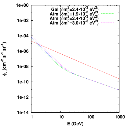
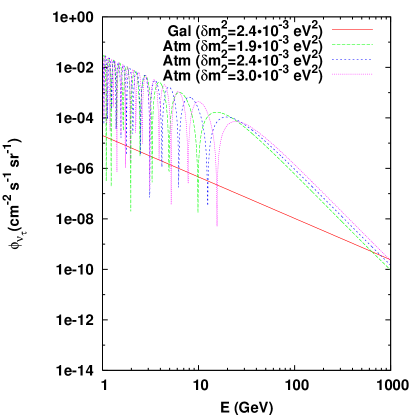
Figure 1: The comparison of galactic-plane and the atmospheric $\nu_{\tau}$ fluxes in the presence of neutrino oscillations. The atmospheric $\nu_{\tau}$ fluxes in the left figure are the downward, while those in the right figure are the upward.

$L_{\rm osc}\equiv 4E/\delta m^{2}\approx 330$ km for $E=1$ GeV and $\delta m^{2}=2.4\cdot 10^{-3}$ eV², we approximate $\sin^{2}(L/L_{\rm osc})$ with $(L/L_{\rm osc})^{2}$, so that $\phi^{\rm tot}_{\nu_{\tau}}(E)\sim\phi_{\nu_{\mu}}(E)E^{-2}$. Because the neutrino oscillation effect steepens the $\phi_{\nu_{\tau}}$ spectrum for $E\leq 20$ GeV, the slope change of $\phi_{\nu_{\tau}}$ at $E\approx 20$ GeV is therefore significant. The plot on the right hand side of Fig. 1 compares the galactic-plane $\nu_{\tau}$ flux and upward atmospheric background flux. The two fluxes cross at $E=8\cdot 10^{2}$ GeV for the best-fit neutrino oscillation parameters. We have also compared the galactic-plane and atmospheric $\nu_{\tau}$ fluxes for several other zenith angles. For instance, for the zenith angle $\xi=60^{\circ}$, these two fluxes cross at $E=6.0$ GeV for $\delta m^{2}=2.4\cdot 10^{-3}$ eV² with the maximal mixing.

The above comparison of galactic-plane and atmospheric $\nu_{\tau}$ fluxes indicates a window of opportunity for the tau neutrino astronomy. Clearly, if $\nu_{\tau}$ can be identified from the overwhelming $\nu_{\mu}$ background (in this case the atmospheric $\nu_{\mu}$ flux), the galactic-plane can be seen through GeV energy tau neutrinos in the downward directions. In the upward directions, galactic-plane tau neutrinos are observable for $E\geq 10^{3}$ GeV.

It is instructive to also compare the galactic-plane and the atmospheric $\nu_{\mu}$ fluxes. While the galactic-plane neutrino flux is flavor independent, the atmospheric $\nu_{\mu}$ flux dominates its $\nu_{\tau}$ counterpart. As a consequence, the crossing point of galactic-plane and atmospheric $\nu_{\mu}$ fluxes is pushed up to $5\cdot 10^{5}$ GeV, which is drastically different from $\nu_{\tau}$ case $\!{}^{{\bf?},{\bf?}}$. This is a general situation in the $\nu_{\mu}$ astronomy where the opportunity for observing astrophysical neutrinos begins typically at $10^{6}$ GeV. In contrast, with the future development of $\nu_{\tau}$ identification techniques, the energy threshold for the neutrino astronomy might significantly be lowered down.

References

References

- [1] Y. Ashie et al. [Super-Kamiokande Collaboration], Phys. Rev. Lett. 93, 101801 (2004).
- [2] Y. Suzuki, in Proceedings of the 28th International Cosmic Ray Conferences (ICRC 2003), ed. T. Kajita et al. (Universal Academic Press, Inc., Tokyo, Japan, 2004), Vol. 8, p. 75.
- [3] T. Kajita and Y. Totsuka, Rev. Mod. Phys. 73, 85 (2001). For a recent discussion, see, A. B. McDonald et al., Rev. Sci. Instrum. 75, 293 (2004).
- [4] J. G. Learned and S. Pakvasa, Astropart. Phys. 3, 267 (1995).
- [5] H. Athar, G. Parente and E. Zas, Phys. Rev. D 62, 093010 (2000).
- [6] T. Stanev, Phys. Rev. Lett. 83, 5427 (1999).
- [7] S. I. Dutta, M. H. Reno and I. Sarcevic, Phys. Rev. D 62, 123001 (2000).
- [8] T. K. Gaisser and M. Honda, Ann. Rev. Nucl. Part. Sci. 52, 153 (2002).
- [9] T. K. Gaisser, Astropart. Phys. 16, 285 (2002).
- [10] H. Athar, K. Cheung, G. L. Lin and J. J. Tseng, Astropart. Phys. 18, 581 (2003).
- [11] H. Athar, F. F. Lee and G. L. Lin, Phys. Rev. D 71, 103008 (2005).
- [12] L. Pasquali and M. H. Reno, Phys. Rev. D 59, 093003 (1999).
- [13] T. K. Gaisser and T. Stanev, Phys. Rev. D 57, 1977 (1998).
- [14] H. Athar, K. Cheung, G. L. Lin and J. J. Tseng, Eur. Phys. J. C 33, S959 (2004).