The Fate of Non-Abelian Plasma Instabilities in 3+1 Dimensions

Abstract

Plasma instabilities can play a fundamental role in plasma equilibration. There are similarities and differences between plasma instabilities in abelian and non-abelian gauge theories. In particular, it has been an open question whether non-abelian self-interactions are the limiting factor in the growth of non-abelian plasma instabilities. We study this problem with 3+1 dimensional numerical simulations. We find that non-abelian plasma instabilities behave very differently from abelian ones once they grow to be non-perturbatively large, in contrast with earlier results of 1+1 dimensional simulations. In particular, they grow more slowly at late times, with linear rather than exponential dependence of magnetic energy on time.

I Introduction

A fundamental problem in the theoretical study of quark-gluon plasmas (QGPs) is to understand how such plasmas equilibrate. By what processes would a heavy ion collision first produce a quark-gluon plasma that is in approximate local equilibrium and/or expanding hydrodynamically? At the very least, it would be useful and interesting to answer this question in a simplifying theoretical limit: that of arbitrarily high-energy collisions, where the running strong coupling $\alpha_{\rm s}$ at relevant scales is arbitrarily small due to asymptotic freedom. Even this weak-coupling limit is rich and complicated. Various authors have used weak-coupling techniques to study the initial creation and interaction of the non-perturbatively dense small-$x$ glue which will eventually develop into the quark-gluon plasma saturate1 ; saturate2 ; saturate3 ; saturate4 ; saturate5 ; saturate6 ; saturate7 . Baier et al. BMSS have investigated the effects of two-particle scattering and Bremsstrahlung on subsequently equilibrating the plasma, once the initial small-$x$ glue has expanded and diluted to perturbative densities, where it can be treated as a collection of individual gluons. However, it now seems clear that the process of thermalization is not controlled solely by such individual particle collisions in the weak-coupling limit ALM ; one must account for collective processes in the plasma in the form of plasma instabilities. The instabilities are known as Weibel or filamentary instabilities weibel , and they have a very long history in traditional plasma physics. Their possible relevance to QGP equilibration has been proposed for roughly twenty years by Mrówczyński and others heinz_conf ; mrow0 ; selikhov1 ; selikhov2 ; selikhov3 ; pavlenko ; mrow1 ; mrow2 ; mrow3 ; mrow&thoma ; randrup&mrow ; strickland .

In the case of electromagnetism, a simple example of a Weibel instability appears for two uniform, interpenetrating beams of charged particles traveling in opposite directions, as depicted in Fig. 1a. Crudely think of each beam as a superposition of many wires carrying current, and recall that parallel wires magnetically attract if their currents are aligned, or repel if opposite. The “wires” are therefore unstable to clumping, as depicted in Fig. 1b. More thorough discussions of the qualitative origin of Weibel instabilities may be found in Refs. mrow3 ; chen and ALM . Very roughly speaking, Weibel instabilities occur in collisionless plasmas whenever the velocity distribution of the plasma is anisotropic in its rest frame. (See Ref. ALM for a more precise statement.) For the purpose of analyzing the instability, the plasma may be regarded as collisionless whenever the distance and time scales associated with the instability are found to be small compared to those for individual, random collisions of particles in the plasma.

Figure 1: (a) Two uniform, inter-penetrating beams of charged particles, moving left and right; (b) the filamentation of those beams by the Weibel instability.

There are magnetic fields associated with the filaments in Fig. 1b. As the instability progresses, these fields become stronger and stronger. Growth of the instabilities is initially exponential in time. In electromagnetic plasmas, growth stops only when the magnetic fields become so large that they have a non-perturbatively large effect on the particle trajectories. These effects of these large fields can drive isotropization of plasmas that are initially anisotropic califano . This isotropization due to collective plasma phenomena is the basis of our own recent scenario (with Lenaghan) for the early onset of hydrodynamic behavior in the weak coupling limit instability_prl , as compared to estimates based on individual 2-particle collisions. To analyze correctly the effects of plasma instabilities, however, it is crucial to understand whether the (chromo-)magnetic fields grow as large in non-abelian gauge theories as in abelian ones. Because non-abelian fields interact with each other, there are two possibilities for what might limit their growth. They might stop growing when (i) their effect on typical particles in the plasma becomes non-perturbative, as in the abelian case, or (ii) when their interactions with each other become non-perturbative. The first case occurs when gauge fields $A$ and magnetic fields $B$ are of order AL

$$A\sim\frac{p_{\rm part}}{g}\qquad\mbox{and}\qquad B\sim\frac{k_{\rm field}\,p_{\rm part}}{g},$$ (1)

where $p_{\rm part}$ is the typical momentum of the particles, and $k_{\rm field}$ is the wavenumber associated with the Weibel instability. The second case corresponds to

$$A\sim\frac{k_{\rm field}}{g}\qquad\mbox{and}\qquad B\sim\frac{k_{\rm field}^{2}}{g}\,.$$ (2)

For weakly-interacting plasmas at times late enough that the particles have diluted to perturbative densities (number densities small compared to $p_{\rm part}^{3}/\alpha_{s}$), one finds that

$$k_{\rm field}\ll p_{\rm part},$$ (3)

and so the second scale (2) is parametrically smaller than the first (1).

Based on arguments about the form of the magnetic potential energy in anisotropic plasmas, Arnold and Lenaghan AL conjectured that the fields associated with non-abelian plasma instabilities are dynamically driven to line up in color space at the scale (2) when their self-interactions become important, and that they then grow as approximately abelian configurations to the larger scale (1). They tested this conjecture numerically in a simplified 1+1 dimensional toy model of QCD fields in an anisotropic plasma. Subsequently, Rebhan, Romatschke, and Strickland RRS simulated the full hard-loop effective theory of the problem in 1+1 dimensions. They indeed found unabated exponential growth beyond the non-abelian scale (2), although the abelianization of the fields was not as global as that of the earlier toy model simulations.

The purpose of this paper is to investigate, through simulations, whether the full 3+1 dimensional theory behaves similarly. We find significant differences. We will soon discuss the details of precisely what we simulate, but here we give a preview of our results and conclusions. The solid line in Fig. 2 shows the growth of magnetic energy with time for a representative simulation. For comparison, the dashed line shows a similar 3+1 dimensional abelian simulation, and the dotted line a 1+1 dimensional non-abelian simulation. In the lower-left shaded region of the plot, the fields are perturbative, and all the curves grow at an exponential rate (as predicted by linearized analysis of the instability). For the non-abelian curves, a change takes place in the unshaded region, which turns out to roughly correspond to the non-abelian scale (2) where self-interactions of the fields become important. The 1+1 dimensional non-abelian simulation soon resumes exponential growth. The 3+1 dimensional non-abelian simulation, however, has a different large-time behavior. Though the magnetic energy continues to grow with time, it eventually becomes linear with time, rather than exponential, in the upper-right shaded region of Fig. 2. This can be seen more clearly in the linear-axis plot of Fig. 3.

Figure 2: A representative simulation of instability growth for 3+1 dimensional SU(2) gauge theory (solid line), 3+1 dimensional abelian gauge theory (dashed line), and 1+1 dimensional SU(2) gauge theory (dotted line). The latter is qualitatively similar to the results of Ref. RRS . The parameters used for these simulations are explained in Sec. II. For 3+1 dimensions, they are $l_{\rm max}=24$, lattice spacing $a=0.25\,m_{\infty}^{-1}$, time step $0.1\,a$, volume $L^{3}=(64\,a)^{3}=(16\,m_{\infty}^{-1})^{3}$, and initial amplitude $\Delta=0.02\,m_{\infty}^{-1/2}$. For 1+1 dimensions, they are the same except that the length is $L=8192\,a=2048\,m_{\infty}^{-1}$ and $\Delta=0.014\,m_{\infty}^{+1/2}$. To simplify comparison of the curves, we have lined them up at early times by shifting the origin of time for the solid and dashed lines, which depend on details of initialization.

Figure 3: Same as Fig. 2, except that the vertical axis is linear rather than logarithmic, and the time axis has been extended.

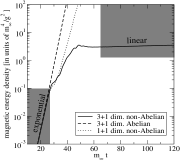
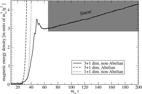
As we shall explain below, the hard-loop effective theory that we simulate treats the plasma particles as having arbitrarily large momentum, $p_{\rm part}\to\infty$, and so the ultimate scale (1) limiting growth of magnetic fields is pushed off to infinity and irrelevant to the interpretation of our results. These simulations are designed for the sole purpose of cleanly studying what happens as one passes through the non-abelian scale (2). For similar reasons, the dependence of our results on $g$ is determined by trivial scaling arguments: In the effective theory we use, all dependence on $g$ can be absorbed by simple rescaling. The only assumptions are that $g$ is small enough, and the separation (3) of scales significant enough, for the hard-loop effective theory to be valid. Given these assumptions, the numerical results we quote are valid for any $g$.

The primary motivation of studying instabilities in non-Abelian plasmas is to help understand what happens in an expanding quark-gluon plasma produced in a heavy-ion collision. In this work, however, we simulate non-expanding systems, both for simplicity and to isolate the particular issue we are studying. Ignoring the expansion is a perfectly good approximation in cases where the instability growth rate is large compared to the expansion rate. For example, in the context of the original “bottom-up” thermalization scenario of Baier et al. BMSS , this approximation would be valid ALM for the initial, exponential growth of instabilities at times late compared to the saturation time scale $1/Q_{\rm s}$ which characterizes the initial moments of the collision. (The saturation momentum scale $Q_{\rm s}$ characterizes the momenta of the original, non-perturbative, small-$x$ gluons that eventually develop into the quark-gluon plasma in the saturation picture.)

The rest of this paper gives details of our simulations. In Sec. II, we explain our formulation and discretization of the hard-loop effective theory and our choice of initial conditions. Sec. III gives further simulation results that aid in understanding the nature of the instability in the non-perturbative regime. In Sec. IV, we discuss sources of systematic errors in our simulations and argue that the qualitative behavior shown in Fig. 3 is not a simulation artifact. Finally, we offer some last thoughts in Sec. V. Some technical results used in the paper are left for appendices.

II What we simulate

II.1 Equations of motion

As in the 1+1 dimensional studies of Rebhan et al. RRS , the starting point for our 3+1 dimensional simulations will be hard-loop effective theory braaten&pisarski ; MRS . This is equivalent to studying kinetic theory of particles in the plasma, coupled to soft gauge fields, in an approximation where the effect of the soft fields on particle trajectories is taken to be perturbative mrowKinetic ; HeinzKinetic ; BIkinetic ; kelly . This description is valid when there is a separation of scales $k_{\rm soft}\ll p_{\rm part}$ as in (3), and when the soft fields have not reached the ultimate limiting amplitude (1). Excitations with momenta of order $p_{\rm part}$ (e.g. the initial post-collision gluons that provide the starting point for the formation of the quark-gluon plasma) are grouped together and described by a classical phase space density $f({\bm{p}},{\bm{x}},t)$. The softer fields associated with the instability, with momenta of order $k_{\rm soft}$, are described by classical gauge fields. Studying the instability by treating these fields as classical is a good approximation because the instability quickly drives the fields to become classically large.

Our formulation of the continuum effective theory, presented below, is equivalent to that used by Rebhan et al. The theory must be discretized for simulations, and we use a different method for discretizing velocity space than Rebhan et al., which we describe below.

We start with the usual kinetic theory description of a collisionless plasma in terms of $f({\bm{x}},{\bm{p}},t)$ and soft gauge fields $A_{\mu}({\bm{x}},t)$. Then write $f=f_{0}({\bm{p}})+\delta f({\bm{p}},{\bm{x}},t)$ and linearize the theory in $\delta f$, which corresponds to a perturbative treatment of the effect of soft fields on hard particles. The result is well known to have the form mrowKinetic

$$[(D_{t}+{\bm{v}}\cdot{\bm{D}}_{\bm{x}})\,\delta f]_{a}+g\,({\bm{E}}+{\bm{v}}\times{\bm{B}})_{a}\cdot{\bm{\nabla}}_{{\bm{p}}}f_{0}=0\,,$$ (4a)

$$(D_{\nu}\,F^{\mu\nu})_{a}=j^{\mu}_{a}\equiv gt_{R}\,\int\frac{d^{3}p}{(2\pi)^{3}}\>v^{\mu}\,\delta f_{a}\,,$$ (4b)

where $\delta f$ is in the adjoint color representation and $a$ is an adjoint color index. Here $D$ is the adjoint-representation gauge-covariant derivative. The group factor $t_{R}$ is defined by $\operatorname{tr}(T_{R}^{a}T_{R}^{b})=t_{R}\delta_{ab}$, where $T_{R}$ is the color generator for the color representation $R$ of the particles, and there is an implicit sum over particle species and spins in (4b). We use $({-}{+}{+}{+})$ metric convention.

For ultra-relativistic plasmas, it is possible to integrate out the dependence on $|{\bm{p}}|$ by defining

$$W_{a}({\bm{v}},{\bm{x}})=gt_{R}\int_{0}^{\infty}\frac{4\pi p^{2}\>dp}{(2\pi)^{3}}\>\delta f_{a}(p{\bm{v}},{\bm{x}},t),$$ (5)

where ${\bm{v}}=\hat{\bm{p}}$ is a unit vector. Eqs. (4) then imply

$$(D_{t}+{\bm{v}}\cdot{\bm{D}}_{\bm{x}})\,W+g^{2}t_{R}({\bm{E}}+{\bm{v}}\times{\bm{B}})\cdot\int_{0}^{\infty}\frac{4\pi p^{2}\>dp}{(2\pi)^{3}}\>{\bm{\nabla}}_{{\bm{p}}}f_{0}=0\,,$$ (6)

$$D_{\nu}\,F^{\mu\nu}=j^{\mu}=\int_{\bm{v}}v^{\mu}W\,,$$ (7)

where $\int_{\bm{v}}$ indicates integration over the unit sphere, normalized so that

$$\int_{\bm{v}}1=\int\frac{d\Omega_{\bm{v}}}{4\pi}=1.$$ (8)

It turns out that these equations only depend on $f_{0}$ through the angular function

$${\cal M}({\bm{v}})\equiv g^{2}t_{R}\int_{0}^{\infty}\frac{4\pi p^{2}\>dp}{(2\pi)^{3}}\>\frac{f_{0}(p{\bm{v}})}{p}\,,$$ (9)

which was introduced in Ref. ALM . Specifically, we show in Appendix A that (6) can be rewritten as

$$(D_{t}+{\bm{v}}\cdot{\bm{D}}_{\bm{x}})\,W+[{\bm{E}}\cdot({\bm{\nabla}}_{\bm{v}}-2{\bm{v}})-{\bm{B}}\cdot({\bm{v}}\times{\bm{\nabla}}_{\bm{v}})]{\cal M}=0,$$ (10)

where ${\bm{\nabla}}_{\bm{v}}$ is the gradient operator for the two-dimensional curved space $S^{2}$ of ${\bm{v}}$’s. More concretely, ${\bm{\nabla}}_{\bm{v}}$ can be related to the ordinary three-dimensional gradient by writing

$$\nabla_{\bm{v}}^{i}=(\delta^{ij}-v^{i}v^{j})|{\bm{p}}|\nabla_{\bm{p}}^{j}$$ (11)

and

$${\bm{\nabla}}_{\bm{v}}\>{\cal M}({\bm{v}})=|{\bm{p}}|{\bm{\nabla}}_{\bm{p}}\>{\cal M}\!\left(\frac{{\bm{p}}}{|{\bm{p}}|}\right).$$ (12)

Everything relevant about the initial distribution is specified by the angular function ${\cal M}({\bm{v}})$. This can be split into a single dimensionful scale

$$m_{\infty}^{2}\equiv\int_{\bm{v}}{\cal M}$$ (13)

and a dimensionless angular function

$$\Omega({\bm{v}})\equiv\frac{{\cal M}({\bm{v}})}{m_{\infty}^{2}}.$$ (14)

The mass $m_{\infty}$ turns out to be the effective mass in the dispersion relation $\omega^{2}\simeq p^{2}+m_{\infty}^{2}$ for large-momentum transverse plasmons ($p\gg m_{\infty}$) boltzmann . In the isotropic case, $\Omega=1$ and $m_{\infty}=m_{\rm D}/\sqrt{2}$, where $m_{\rm D}$ is the Debye mass.

In order to discretize the problem for simulation, we generalize the procedure used by Bödeker, Moore, and Rummukainen BMR for the isotropic case. Specifically, we will discretize the 2-dimensional velocity space by expanding functions of ${\bm{v}}$ in spherical harmonics $Y_{lm}({\bm{v}})$ and truncating at some maximum value $l_{\rm max}$ of $l$. We will have to check later, of course, that our simulation results are insensitive to the exact value of $l_{\rm max}$ used, provided it is large enough. So, we write

$$W^{a}({\bm{v}})=\sum_{l\leq l_{\rm max}}\sum_{m}W^{a}_{lm}\,\bar{Y}_{lm}({\bm{v}}),$$ (15a)

$$\Omega({\bm{v}})=\sum_{l\leq l_{\rm max}}\sum_{m}\Omega_{lm}\,\bar{Y}_{lm}({\bm{v}}),$$ (15b)

where we have chosen to normalize spherical harmonics without the usual factor of $\sqrt{4\pi}$, so that $\bar{Y}_{00}=1$ and

$$\int_{\bm{v}}\bar{Y}_{lm}({\bm{v}})^{*}\,\bar{Y}_{l^{\prime}m^{\prime}}({\bm{v}})=\delta_{ll^{\prime}}\,\delta_{mm^{\prime}}\,.$$ (16)

The bar over the $Y$ serves as a reminder of this normalization. For working in $lm$-space, it is convenient to rewrite the equation (10) for $W$ in the equivalent form (discussed in Appendix A)

$$(D_{t}+{\bm{v}}\cdot{\bm{D}}_{\bm{x}})\,W+\bigl{(}{\bm{E}}\cdot({\textstyle{\frac{1}{2}}}[{\bm{v}},L^{2}]-{\bm{v}})-i{\bm{B}}\cdot{\bm{L}}\bigr{)}{\cal M}=0$$ (17)

where

$${\bm{L}}\equiv-i{\bm{v}}\times{\bm{\nabla}}_{\bm{v}}=-i{\bm{p}}\times{\bm{\nabla}}_{\bm{p}}$$ (18)

is the operator, analogous to angular momentum, for which the eigenvalues of $L^{2}$ and $L_{z}$, acting on $\bar{Y}_{lm}({\bm{v}})$, are $l(l+1)$ and $m$. One may then find the coupled equations for the $W_{lm}$’s using manipulations familiar from the quantum mechanics of spin.

In this paper, we will only simulate initial particle distributions $f_{0}({\bm{p}})$ which are axially-symmetric about the $z$ axis, for which there are many simplifications. In this case,

$$\Omega({\bm{v}})=\sum_{l\leq l_{\rm max}}\Omega_{l0}\,\bar{Y}_{l0}({\bm{v}}).$$ (19)

The equations for the $W_{lm}$’s in this case are given explicitly in Appendix A. They are the same as those used by Bödeker et al. BMR except for the ${\bm{E}}$ and ${\bm{B}}$ terms in the $W$ equation (6), which are sensitive to anisotropy in $f_{0}$. With this exception, our discretization of the problem, and the evolution algorithm we use, are identical to Ref. BMR . For computational simplicity, we simulate SU(2) gauge theory instead of SU(3) gauge theory. We do not know of any reason that SU(3) would be qualitatively different. For future reference, we note that the vector current in Maxwell’s equation (7) is determined by the $l{=}1$ components of $W$ as

$$j_{x} = \frac{1}{\sqrt{6}}\,(W_{1,-1}-W_{11})=-\sqrt{\frac{2}{3}}\operatorname{Re}W_{11},$$ (20a)

$$j_{y} = -\frac{i}{\sqrt{6}}\,(W_{1,-1}+W_{11})=\sqrt{\frac{2}{3}}\operatorname{Im}W_{11},$$ (20b)

$$j_{z} = \frac{1}{\sqrt{3}}\,W_{10}.$$ (20c)

We should mention that, in the traditional plasma physics literature, the 1+1 dimensional simulations of Rebhan et al. would be referred to as 1D+3V simulations, indicating that they treat gauge fields and particle distributions as depending on only four of the six dimensions of phase space: one dimension of ${\bm{x}}$ space and three dimensions of momentum (velocity) space. All three spatial components $(A_{x},A_{y},A_{z})$ of 3-dimensional gauge fields ${\bm{A}}$ are simulated in 1D+3V, but they depend on only one spatial dimension, e.g. $A_{i}=A_{i}(t,z)$. The 3+1 dimensional simulations in this paper are correspondingly referred to as 3D+3V. However, in the ultra-relativistic limit, calculations are simplified by the fact that velocity space is effectively 2 dimensional, since $|{\bm{v}}|=1$.

Other 1D+3V simulations of non-abelian plasma instabilities have been performed by Dumitru and Nara Dumitru . Instead of working with a phase space distribution $f$, they simulate a finite number of discrete, classical particles with classical color charges interacting with the soft fields wong ; christina ; hu&muller ; MHM . If one linearizes in the perturbations to the hard particles, this formulation leads to an effective theory equivalent to that above. However, they do no such linearization, since their interest lay in studying what happens if the effects on hard particles eventually become substantial.

II.2 Choice of $f_{0}$

If we measure all quantities in units determined by the single dimensionful scale $m_{\infty}$, then the only sensitivity of our problem to the choice of the initial hard particle distribution $f_{0}({\bm{p}})$ is through the angular function $\Omega({\bm{v}})$. In the axi-symmetric case, that means we have to choose $\Omega(\theta)$, where $\theta$ is the angle of ${\bm{v}}$ with the $z$ axis. In this paper, we will only investigate results for a single choice of $\Omega(\theta)$. Our criteria for choosing this distribution were that (i) perturbatively, the dominant instability should be a Weibel instability; (ii) $\Omega_{lm}$ should be dominated by relatively low $l$’s, to aid in numerical convergence of our simulations to the $l_{\rm max}{\to}\infty$ limit; (iii) the Weibel instability growth rate should be reasonably large (relative to wavelength), to help minimize simulation time; (iv) $\Omega(\theta)$ should be everywhere non-negative, since the distribution $f_{0}$ is; and (v) preferably $\Omega(\theta)$ should be monotonic for $0\leq\theta\leq\pi/2$. The last condition is simply superstition: We did not want to have to worry whether a multiple-hump distribution might perhaps have qualitatively different behavior than a single-hump one, and so we chose to study the simplest, most natural case. After some experimentation with distributions containing only $l\leq 6$ harmonics, we settled on

$$\Omega(\theta)\propto(\cos^{2}\beta-\cos^{2}\theta)^{3}+\sin^{6}\beta\qquad\mbox{with $\beta=0.480$.}$$ (21a)

This corresponds to

$$\Omega_{00}=1\,,\qquad\Omega_{20}=-0.790\,,\qquad\Omega_{40}=0.367\,,\qquad\Omega_{60}=-0.093\,,$$ (21b)

with all other $\Omega_{lm}=0$. Fig. 4 shows a plot of the angular dependence.

Figure 4: The angular dependence $\Omega(\theta)$ of our hard-particle distribution (21).

The dominant instability of this distribution is a Weibel instability with wave-number ${\bm{k}}$ along the $z$ axis. A perturbative analysis of this instability (see Sec. IV.1) shows that the mode with the maximum growth rate $\gamma$, in the infinite-volume, continuum limit, has

$$k=0.827\,m_{\infty},\qquad\gamma=0.273\,m_{\infty}\,.$$ (22)

II.3 Initial conditions

We want to choose initial conditions that (i) have a random mix of perturbatively unstable modes, and (ii) are insensitive to the ultraviolet cutoff so that, for instance, the energy density has a good continuum limit. A simple choice that works in any dimension is to choose Gaussian noise for the gauge fields ${\bm{A}}$ with an exponential fall-off in ${\bm{k}}$:

$${\bm{A}}({\bm{x}})=\int\frac{d^{d}k}{(2\pi)^{d}}\,{\bm{A}}({\bm{k}})\,e^{i{\bm{k}}\cdot{\bm{x}}},$$ (23)

where $d{=}1$ or 3 is the number of spatial dimensions and the $A_{i}^{a}({\bm{k}})$ are Gaussian random variables with variance

$$\langle A_{i}^{a}({\bm{k}})^{*}\,A_{j}^{b}({\bm{k}}^{\prime})\rangle=\left(\frac{\Delta}{g}\,e^{-k^{2}/k_{0}^{2}}\right)^{2}\,\delta^{ab}\delta_{ij}\,(2\pi)^{d}\,\delta^{(d)}({\bm{k}}-{\bm{k}}^{\prime}).$$ (24)

Here $\Delta$ and $k_{0}$ are constants. It is conventional in simulations of SU(2) gauge theory to rescale the definition of fields to absorb factors of $2/g$, but in this paper we will show all factors explicitly. Our simulations are carried out in $A_{0}{=}0$ gauge, but the evolution equations and all the observables we report are gauge invariant. We choose

$${\bm{E}} = -\dot{\bm{A}}=0$$ (25)

and

$$W = 0$$ (26)

as our remaining initial conditions. Both are motivated solely by simplicity. In particular, (25) automatically implements Gauss’ Law.

For small $\Delta$ (so that perturbation theory applies) in three dimensions, these initial conditions correspond to to an initial magnetic energy density of

$$\langle{\textstyle{\frac{1}{2}}}B^{2}\rangle\simeq\frac{3\nu\,k_{0}^{5}}{64\,(2\pi)^{3/2}}\,\frac{\Delta^{2}}{g^{2}}$$ (27)

in the infinite-volume, continuum limit, where $\nu=6$ is the number of gauge boson degrees of freedom [2 spin times 3 color for SU(2)]. In 1D+3V dimensions, the corresponding result is

$$\langle{\textstyle{\frac{1}{2}}}B^{2}\rangle\simeq\frac{\nu\,k_{0}^{3}}{16\,(2\pi)^{1/2}}\,\frac{\Delta^{2}}{g^{2}}\,.$$ (28)

In the 3D+3V dimensional simulations reported in this paper, we choose the momentum cut-off scale $k_{0}$ in (24) as

$$k_{0}=2m_{\infty}.$$ (29)

Unless otherwise stated, we take the initial amplitude $\Delta$ in 3D+3V simulations to be

$$\Delta=0.02\,m_{\infty}^{-1/2}.$$ (30)

In 1D+3V simulations, we take $\Delta=0.014\,m_{\infty}^{+1/2}$, which corresponds to roughly the same value of the dimensionless energy $g^{2}\langle{\textstyle{\frac{1}{2}}}B^{2}\rangle/m_{\infty}^{4}$.

To perform abelian simulations, we use our SU(2) simulation code with initial conditions that lie in a single direction in adjoint color space, i.e.

$$\langle A_{i}^{a}({\bm{k}})\,A_{j}^{b}({\bm{k}}^{\prime})\rangle=\left(\frac{\Delta}{g}\,e^{-k^{2}/k_{0}^{2}}\right)^{2}\,\delta^{a3}\delta^{b3}\delta_{ij}\,(2\pi)^{d}\,\delta^{(d)}({\bm{k}}-{\bm{k}}^{\prime}).$$ (31)

III Additional Results

In addition to the magnetic energy plotted in Figs. 2 and 3, it is interesting to see a breakdown of other components of the energy of the soft fields. For an isotropic distribution $f_{0}$, the combination

$$\int_{\bm{x}}\left[{\textstyle{\frac{1}{2}}}E^{2}+{\textstyle{\frac{1}{2}}}B^{2}+{\textstyle{\frac{1}{4}}}\,m_{\infty}^{-2}\int_{\bm{v}}W^{2}\right]$$ (32)

would be conserved Wformalism . We will therefore loosely refer to ${\textstyle{\frac{1}{4}}}\,m_{\infty}^{-2}\int_{\bm{v}}W^{2}$ as the “$W$ field energy density.” Figs. 5 and 6 compare various components of the volume-averaged energy density as a function of time, including the magnetic, electric, and $W$ field energy densities. As one indication of the anisotropy of the soft fields, we also show ${\textstyle{\frac{1}{2}}}B_{z}^{2}$ and ${\textstyle{\frac{1}{2}}}E_{z}^{2}$. Note that, unlike Fig. 2, we now show time all the way back to the initial conditions at $t=0$. There is a very early transient at $m_{\infty}t\lesssim 1$ that is difficult to see in the plot, when the initial energy in the magnetic fields is quickly shared with the other degrees of freedom, $E$ and $W$. The unstable modes start to grow, but it is only when they grow large enough to dominate the energy density that this manifests as the start of exponential growth in the magnetic energy, around $m_{\infty}t\sim$ 10 to 15.

Figure 5: Various components of the energy density for the same three dimensional non-abelian simulation as in Fig. 2.

Figure 6: Same as Fig. 5, but with a linear vertical axis.

Figure 7: The ratio of the $B_{z}^{2}$ contribution to the magnetic energy density to the total $B^{2}$ for the 3+1 and 1+1 dimensional simulations of Fig. 2. To make the curves line up, the time origin of the 1+1 dimensional simulation has been shifted just as in Fig. 2 ($m_{\infty}t\to m_{\infty}t+9.2$).

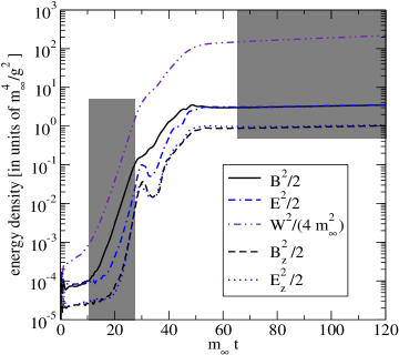
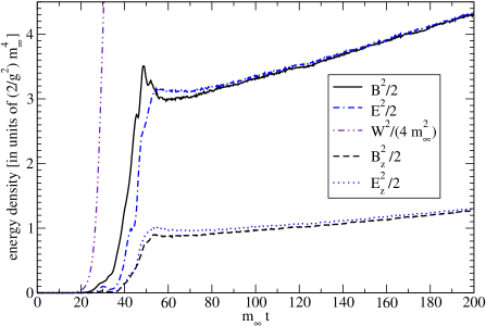
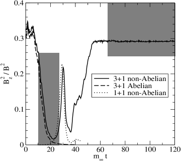
Fig. 7 shows the ratio of the $B_{z}^{2}$ contribution to the magnetic energy density to the total $B^{2}$. If the soft fields were isotopic, this ratio would be $1/3$. This is indeed the value at the earliest times, due to our isotropic soft-field initial conditions. For $10\lesssim m_{\infty}t\lesssim 20$, as the Weibel instability first starts to grow and dominate the magnetic field, $B_{z}$ drops dramatically compared to $B$. This is because the Weibel instability is dominated by modes with wavenumber ${\bm{k}}$ along the $z$ axis, and magnetic fields are perpendicular to ${\bm{k}}$. In the abelian case, that is the end of the story: $B_{z}$ continues to become more and more insignificant as the unstable modes grow. In the non-abelian case, $B_{z}=({\bm{\nabla}}\times{\bm{A}})_{z}-ig[A_{x},A_{y}]$, and the non-abelian commutator contributes even when ${\bm{k}}$ is in the $z$ direction. This contribution to $B_{z}$ will grow with time, as the gauge fields $A_{x}$ and $A_{y}$ grow due to the instability, and $B_{z}$ should become the same order of magnitude as $B_{x}$ and $B_{y}$ once those fields become non-perturbatively large (2). This growth corresponds to roughly $23<m_{\infty}t<30$ in the figure. At $m_{\infty}t\sim 30$, the ratio is no longer small, and so one would expect this to be where some deviation from the behavior of abelian instabilities should occur. This was indeed the case in the non-abelian magnetic energy curve of Figs. 2 and 5, where one sees a first small bump in the plot of magnetic energy vs. time at $m_{\infty}t\sim 30$.

Based on arguments concerning 1+1 dimensional configurations of fields, it was conjectured in Ref. AL that dynamics at the non-abelian scale would cause the field configurations to approximately abelianize, and that the Weibel instability would then again take over, causing the field to grow all the way to the ultimate scale (1). If abelian-like Weibel modes come to dominate, then $B_{z}$ should again become small relative to $B$. This was seen in numerical simulations by Rebhan et al. and is reproduced in our own 1+1 dimensional data in Fig. 7 for $m_{\infty}t>30$. For a brief time, the $3+1$ dimensional simulations behave similarly, but the decrease of $B_{z}/B$ eventually stops and reverses at $m_{\infty}t\sim 36$. The ratio then starts growing again and finally levels out near 0.29 (slightly lower than one third) at $m_{\infty}t\sim 53$, which is near the beginning of the linear growth of magnetic energy in Figs. 3 and 6.

Figure 8: The ratio of electric to magnetic energy.

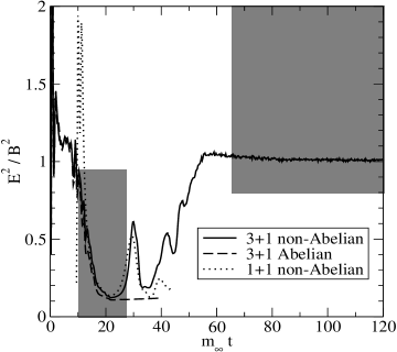
In Fig. 8, we plot the ratio of electric energy to magnetic energy. The behavior is somewhat similar to the previous plot. Looking at the abelian curve (dashed), we see that, as the Weibel instability grows and dominates the energy density, the ratio drops and eventually asymptotes to a constant. Theoretically, this constant should be $(\gamma/k)^{2}$, where $\gamma$ and $k$ are the growth rate and wave number of the dominant unstable mode. Using (22), the infinite-volume, continuum value is $(\gamma/k)^{2}=0.11$, which is in good agreement with the figure. For the non-abelian simulations, however, the ratio subsequently grows as non-abelian interactions first become important, and then decreases again, consistent with the picture of approximate abelianization. For 3+1 dimensional non-abelian simulations, however, the ratio then increases yet again, and finally approaches unity in the linear energy growth regime. Note that plasma oscillations with momenta large compared to the mass $m_{\infty}$ would naturally have $E^{2}{\simeq}B^{2}$. Fig. 8 might therefore be a hint about what sort of soft field excitations dominate the energy in the linear regime.

It is interesting to directly address the conjecture of Ref. AL that non-perturbative dynamics would abelianize the gauge field configurations. We consider the following local observable, related to ones used by Refs. AL ; RRS :

$$C\equiv\frac{3}{\sqrt{2}}\>\frac{\left[\int\frac{d^{3}x}{V}\>\Bigl{(}([j_{x},j_{y}])^{2}+([j_{y},j_{z}])^{2}+([j_{z},j_{x}])^{2}\Bigr{)}\right]^{1/2}}{\int\frac{d^{3}x}{V}\>|{\bm{j}}|^{2}}\,,$$ (33)

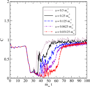
where $[j_{x},j_{y}]^{2}\equiv\epsilon^{abc}j^{b}_{x}j^{c}_{y}\,\epsilon^{amn}j^{m}_{x}j^{n}_{y}$, etc. The normalization of $C$ has been chosen so that $C$ would be unity if the components of ${\bm{j}}$ were independent random numbers with the same distribution. For an abelian configuration, $C$ would be zero. Fig. 9 shows the time development of $C$ in our canonical non-abelian simulations. We see that $C$ drops suddenly when non-abelian interactions first become important, in agreement with the abelianization conjecture. However, in the 3+1 dimensional simulations, $C$ later rises again all the way to unity, showing no local abelianization in the linear growth regime.

Figure 9: The local measure (33) of the relative size of commutators, plotted as a function of time, for the non-abelian simulations of Fig. 2.

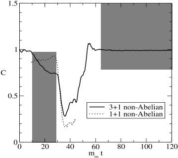
In Figs. 7–9, we have not displayed any data for the 1+1 non-abelian or 3+1 abelian simulations at late times when the corresponding energy curves in Fig. 2 grew so large that they are approaching the top of the plot. At those and later times, the fields in our simulations grow so large that they become sensitive to the discretization of the lattice, and the behavior of the results is then a lattice artifact. We shall discuss this issue more thoroughly in Sec. IV.3.

Figure 10: A comparison of magnetic energy density (solid) and the average squared current $|{\bm{j}}|^{2}$ (dashed), with the latter normalized as in (34), for the 3+1 dimensional non-Abelian simulation of Fig. 2.

Figure 11: Same as Fig. 10, but with a linear vertical axis.

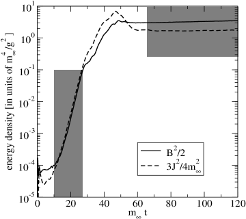
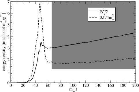
In 1+1 dimensional simulations, the size of particle currents ${\bm{j}}$ was used by Rebhan et al. RRS to track the growth of the instability. In Figs. 10 and 11, we track a related quantity for our 3+1 dimensional simulations. These figures compare the magnetic energy density to the energy density in the $l{=}1$ components of $W$. The latter is given by (32) as $W_{1m}^{a}W_{1m}^{a}/(4m^{2}_{\infty})$, which is directly proportional to the squared current $|{\bm{j}}|^{2}$ by (20):

$$\frac{1}{4m_{\infty}^{2}}\sum_{m}W_{1m}^{a}W_{1m}^{a}=\frac{3|{\bm{j}}|^{2}}{4m_{\infty}^{2}}\,.$$ (34)

Fig. 11 shows that $\frac{3}{4}\,|{\bm{j}}|^{2}/m_{\infty}^{2}$ exceeds the magnetic energy ${\textstyle{\frac{1}{2}}}{\bm{B}}^{2}$ by roughly a factor of two in the exponential growth regime, but then drops substantially and is only about half the magnetic energy in the linear regime.

IV Checks and systematic errors

IV.1 Perturbative growth rate

One simple check of simulations is to see whether the rate of exponential energy growth in the perturbative regime is consistent with the infinite-volume, continuum prediction for the Weibel instability growth rate. To compute the perturbative growth rate, one looks for exponentially growing solutions ($\operatorname{Im}\omega>0$) to the linear dispersion relation

$$[(-\omega^{2}+k^{2})g^{\mu\nu}-K^{\mu}K^{\nu}+\Pi^{\mu\nu}(\omega,{\bm{k}})]A_{\nu}=0,$$ (35)

where $K=(\omega,{\bm{k}})$ and $\Pi$ is the hard loop self-energy mrow0 ; randrup&mrow

$$\Pi^{\mu\nu}(\omega,{\bm{k}}) = g^{2}t_{R}\int_{\bm{p}}\frac{\partial f_{0}({\bm{p}})}{\partial p^{\,l}}\left[-v^{\mu}g^{l\nu}+\frac{v^{\mu}v^{\nu}k^{l}}{-\omega+{\bm{v}}\cdot{\bm{k}}-i\epsilon}\right].$$ (36)

In Appendix B, we formulate this in terms of the angular distribution ${\Omega({\bm{v}})}$ and then find a result that is well suited for calculations of growth rates in cases where $\Omega$ is expressed in terms of spherical harmonics. Specifically, in situations where the hard particle distribution $f_{0}({\bm{p}})$ is axi-symmetric, the transverse self-energy for wave-vectors along the $z$ axis can be expressed as

$$\Pi_{\perp}(\omega,k{\bm{e}}_{z})={\textstyle{\frac{1}{2}}}m_{\infty}^{2}\sum_{l}\sqrt{2l{+}1}\;\kappa_{l}\!\left(\frac{\omega}{k}\right)\,{\Omega_{l0}}$$ (37a)

with

$$\kappa_{l}(\eta)\equiv(1+\eta^{2})\delta_{l0}+(1-\eta^{2})[(l+1)Q_{l+1}(\eta)-(l-1)\eta Q_{l}(\eta)].$$ (37b)

Here, $Q_{l}(\eta)$ is the Legendre function of the second kind defined so that it is regular at $\eta=\infty$ and the cut is chosen to run from $-1$ to +1. In cases where the dominant instability is a Weibel instability with ${\bm{k}}$ along the axis of symmetry, the dispersion relation then reduces to

$$-\omega^{2}+k^{2}+\Pi_{\perp}(\omega,k{\bm{e}}_{z})=0.$$ (38)

For a given distribution $\Omega(\theta)$, one can solve this equation numerically for each $k$, and then scan over $k$ to look for the mode with the largest growth rate $\gamma=\operatorname{Im}\omega$. For the distribution (21) used in our simulations, the resulting $\gamma$ and $k$ were given earlier in Eq. (22).

Figure 12: The perturbative growth in Fig. 2 compared to the predicted growth (39) of the dominant Weibel mode (22). As in previous figures, we have shifted the time origin of the 1+1 dimensional simulation to line up the curves ($m_{\infty}\to m_{\infty}t+9.2$).

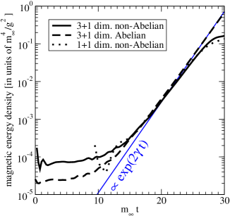
The rate $\gamma$ gives the growth rate of the perturbative vector potentials. The corresponding magnetic energy should grow as the square of the field strength, so that

$${\textstyle{\frac{1}{2}}}B^{2}\propto e^{2\gamma t}.$$ (39)

In Fig. 12, we again show our canonical simulations of Fig. 2, this time focusing on the perturbative regime and comparing the slope of $\ln({\textstyle{\frac{1}{2}}}B^{2})$ to $2\gamma$. We get reasonable agreement. Keep in mind that there is an entire spectrum of unstable modes, not just the dominant mode discussed above; so the exponential growth of instabilities is not described by a single exponential at early times.

IV.2 Finite volume errors

In Figs. 13 and 14, we show how our 3+1 dimensional non-abelian simulation results of Fig. 2 change if we decrease the physical volume. When comparing results for different volumes, it is important to realize that different simulations will have different random initial conditions—there is no good way to start two simulations with the same initial conditions when they have different physical volumes. To get an idea of the size of this effect, we have simulated various volumes more than once, changing the seed of our random number generator. For very large volumes, one would expect the spread of the results to decrease with increasing volume because the volume average taken in computing the energy density averages over multiple spatial regions with different initial conditions.

Figure 13: Magnetic energy vs. time as in Fig. 2, but showing results for several different physical volumes. Multiple lines for a single volume correspond to different instantiations of the random initial conditions.

Figure 14: Same as Fig. 13, but with a linear vertical axis.

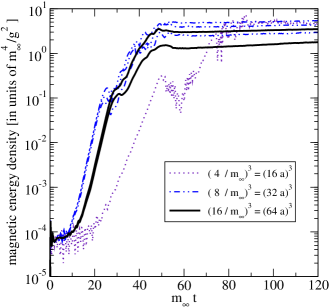
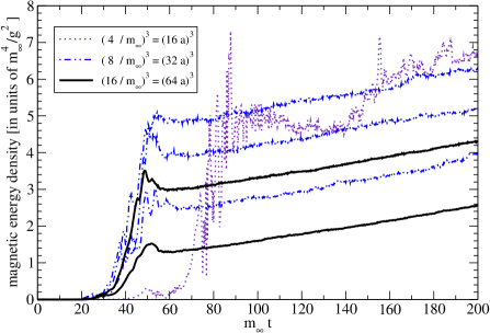
As one can see, the simulations shown in Fig. 14 still show a significant variation in results with respect to initial conditions at a volume of $L^{3}=(16/m_{\infty})^{3}$. However, the rates of growth in the perturbative, exponential regime and the non-perturbative, linear regime have clearly reached their large volume limits. Specifically, Fig. 13 shows that the perturbative growth rate (the slope of the curve for $10\lesssim m_{\infty}\lesssim 20$) is not significantly affected in increasing volume from $(8/m_{\infty})^{3}$ to $(16/m_{\infty})^{3}$. And Fig. 14 similarly shows little effect on the slope of the late-time linear growth behavior. This implies that the phenomenom of linear growth is not a finite-volume artifact.

IV.3 Finite lattice spacing errors

IV.3.1 3+1 dimensions

Fig. 15 shows the lattice spacing dependence of our simulations for a lattice volume of $L^{3}=(8/m_{\infty})^{3}$. We chose a smaller volume than that used in our canonical simulation of Fig. 2 so that we could push to smaller lattice spacing with our available computer resources. Recall from Fig. 13 that this smaller volume is adequate for reproducing the linear growth rate. Here and in all our simulations, the time step used in evolving the system is $\delta t=0.1\,a$. 

Figure 15: Magnetic energy vs. time as in Fig. 2, but showing results for several different choices of lattice spacing for a volume $L^{3}=(8/m_{\infty})^{3}$. The $a{=}0.25\,m_{\infty}^{-1}$ and $a{=}0.125\,m_{\infty}^{-1}$ curves are difficult to distinguish on this plot.

Figure 16: Same as Fig. 15, but with a linear vertical axis.

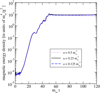
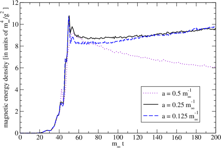
Since we have already seen that different initial conditions can produce substantially different behaviors at this volume, especially at the transition between exponential and linear growth, it is essential in comparing lattice spacings to ensure that the initial conditions are as nearly identical as possible. In Figures 15 and 16, we have done this by drawing the smallest lattice spacing configuration randomly as described in subsection II.3, and converting it into larger lattice spacing configurations via blocking. Besides the lattice spacing and volume, we otherwise use the same “canonical” values for variables as in most previous simulations.

From Fig. 15, one sees negligible spacing dependence in the early, perturbative growth of the instability. From Fig. 16, we conclude that spacing does not have a significant effect effect on the slope of the linear growth in magnetic energy provided $a$ is at least as small as our canonical value of $0.25\,m_{\infty}^{-1}$. The largest lattice spacing shows approximately the same exponential growth behavior, but different linear growth behavior. This is apparently because there is more energy in ultraviolet degrees of freedom during the linear growth period, and these degrees of freedom are compromised by the large lattice spacing.

To test dependence on both lattice spacing and initial amplitude $\Delta$, we show in Fig. 17 what happens if we start with large, non-perturbative initial conditions of $\Delta=2.0$. Here the system goes directly into linear growth, and the $a=0.25\,m_{\infty}^{-1}$ and $a=0.125\,m_{\infty}^{-1}$ results are reasonably close.

Figure 17: Lattice spacing dependence for non-perturbatively large initial conditions, $\Delta=2$.

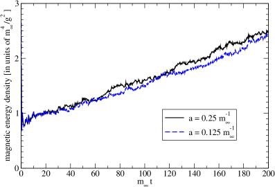
From the consistency of the slope of the linear regime for $a\leq 0.25\,m_{\infty}$, we conclude that the existence of the linear growth regime is not an artifact of finite lattice-spacing.

IV.3.2 1+1 dimensions

To sharpen our conclusions that the linear growth regime in 3+1 dimensions is not an artifact of our simulations, it is useful to look at a different case, where the end of exponential growth is a lattice artifact. Such an example is provided by our 1+1 dimensional simulations, shown in Fig. 18 for a variety of lattice spacings. We display results to much larger energies than in Fig. 2. Superficially, each individual curve looks vaguely similar to our 3+1 dimensional results: each shows an eventual end to exponential growth, although at much higher energy density than in 3+1 dimensions.

In our simulations, we implement 1+1 dimensions by using our 3+1 dimensional code on a periodic lattice that is a single lattice spacing wide in the $x$ and $y$ directions. No matter how fine the lattice is compared to the wavelength of the unstable modes, the continuum limit will break down when the fields become so large that the magnetic energy per plaquette is of order its maximum possible value on the lattice, corresponding to ${\textstyle{\frac{1}{2}}}B^{2}\sim 1/(g^{2}a^{4})$. Even at lower fields, the dynamics is modified by “irrelevant” operators induced by the lattice, such as $a^{2n}B^{n+1}$, which become more and more important as $B$ grows larger. As one takes the lattice spacing $a$ smaller and smaller, the fields should be able to grow larger and larger before these problems arise. The termination of exponential growth in Fig. 18 clearly shows this behavior, demonstrating it is a lattice artifact.

Figure 18: Magnetic energy vs. time for 1+1 dimensional simulations with several different choices of lattice spacing for a system length $L=128/m_{\infty}$. The remaining parameters are as in Fig. 2. except that here we have not shifted the origin of the time axis.

Figure 19: Same as Fig. 18, but the vertical axis is linear and different vertical offsets have been added to each curve to fit them onto the plot. From top to bottom on the left side of the plot, the curves correspond to $am_{\infty}=$ 0.125, 0.25, 0.5, 0.0625, and 0.03125.

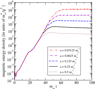
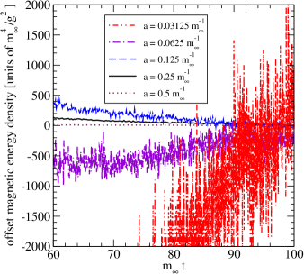
In discussing our 3+1 dimensional simulations, we have emphasized how the slope of the late-time linear growth is not significantly sensitive to decreasing the lattice spacing. In contrast, a similar look at the slope of the phony late-time behavior of the 1+1 simulations, in Fig. 19, shows no such spacing independence.

Fig. 20 shows the measure $C$ of local commutators, defined by Eq. (33), for the 1+1 dimensional simulations of Fig. 18. The reader may now see late-time behavior that we did not display in Fig. 9, and also see that this behavior is a lattice spacing artifact. This is the reason we truncated our 1+1 dimensional curves in Figs. 7–9. Specifically, we truncated those curves when the magnetic energy densities reached $20\,m_{\infty}^{4}/g^{2}$, which is a little before where the $a=0.25\,m_{\infty}^{-1}$ energy curve deviates from the continuum limit in Fig. 18 and where the corresponding curve for $C$ suddenly begins to rise in Fig. 9. A similar truncation was made for the Abelian results, where a similar large-field issue arises since we implement compact rather than non-compact Abelian gauge theory.

Figure 20: The local measure (33) of the relative size of commutators for the various 1+1 dimensional simulations of Fig. 18. From top to bottom, the curves are in descending order in the size of $a$.

IV.4 Finite $l_{\rm max}$ errors

Figs. 21 and 22 show the dependence of our results on $l_{\rm max}$. The figures show simulations with fixed lattice spacing $a=0.25\,m_{\infty}$ and fixed physical volume $L^{3}=(8/m_{\infty})^{3}$. By comparison of the $l_{\rm max}{=}24$ and $l_{\rm max}{=}48$ curves in Fig. 22, we conclude that our canonical choice of $l_{\rm max}=24$ seems to be a good approximation to the large $l_{\rm max}$ limit and that the linear growth regime is not a finite $l_{\rm max}$ artifact.

Figure 21: Magnetic energy vs. time for several different choices of $l_{\rm max}$. These simulations have $a=0.25\,m_{\infty}^{-1}$, $l_{\rm max}=24$, $L^{3}=(32\,a)^{3}=(8\,m_{\infty}^{-1})^{3}$, and $\Delta=0.02\,m_{\infty}^{-1/2}$. The $l_{\rm max}{=}24$ and $l_{\rm max}{=}48$ curves are difficult to distinguish on this plot.

Figure 22: Same as Fig. 21, but with a linear vertical axis. The $l_{\rm max}{=}24$ and $l_{\rm max}{=}48$ curves are again very close together.

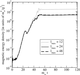
We have chosen to run simulations only for even values of $l_{\rm max}$, based on the experience of Ref. BMR for isotropic particle distributions, where it was found that convergence to the large $l_{\rm max}$ limit was much faster for $l_{\rm max}$ even than $l_{\rm max}$ odd.

V Discussion

We have found that 3D+3V dimensional non-abelian plasma instabilities behave qualitatively differently than 1D+3V dimensional instabilities once they grow non-perturbatively large. Initially, there is a period of non-perturbative growth that looks quite similar to the 1D+3V case and to early conjectures about abelianization, but eventually the 3D+3V instabilities settle into a period characterized by linear rather than exponential growth of the magnetic energy. Based on our analysis of sources of systematic error, we believe that this conclusion is not a simulation artifact.

There are many more things one would like to know about the linear growth regime, such as its efficiency at scattering and isotropizing typical particles in the plasma, its power spectrum, and possible models for the underlying physical processes. It would also be useful to check whether non-perturbative linear growth occurs for a wide variety of different distributions $f_{0}(\theta)$, beyond the single case studied here. We leave this and further characterization to future work.

Appendix A Hard loop effective theory in $lm$-space

First, we will fill in a few steps in the text. The transition from (6) to (10) follows by using (11) to write

$${\bm{\nabla}}_{\bm{p}}f_{0}=\frac{1}{p}\,{\bm{\nabla}}_{\bm{v}}f_{0}+{\bm{v}}\,\frac{\partial f_{0}}{\partial p}\,.$$ (40)

Then integrate the last term by parts in $dp$ to obtain

$$\int_{0}^{\infty}\frac{4\pi p^{2}\>dp}{(2\pi)^{3}}\>{\bm{\nabla}}_{{\bm{p}}}f_{0}=({\bm{\nabla}}_{\bm{v}}-2{\bm{v}}){\cal M}$$ (41)

and so (10). Using (11) and (18), one may derive that

$$[{\bm{v}},L^{2}]=2({\bm{\nabla}}_{\bm{v}}-{\bm{v}}),$$ (42)

which yields (17).

Now use the $lm$-expansions (15) of $W$ and $\Omega$ in (17) and project out the $lm$-th component of the result. Working in $A_{0}{=}0$ gauge, which is the gauge of our simulations, this yields the evolution equation for $W_{lm}$,

$$\partial_{t}W_{lm} = \sum_{l^{\prime}m^{\prime}}\Bigl{\{}-\langle lm|{\bm{v}}|l^{\prime}m^{\prime}\rangle\cdot{\bm{D}}_{x}W_{l^{\prime}m^{\prime}}$$ (43)

$$\hskip 50.00008pt-\left({\bm{E}}\cdot\langle lm|{\textstyle{\frac{1}{2}}}[{\bm{v}},L^{2}]-{\bm{v}}|l^{\prime}m^{\prime}\rangle-i{\bm{B}}\cdot\langle lm|{\bm{L}}|l^{\prime}m^{\prime}\rangle\right)m_{\infty}^{2}\,\Omega_{l^{\prime}m^{\prime}}\Bigr{\}}$$

$$= \sum_{l^{\prime}m^{\prime}}\Bigl{\{}-\langle lm|{\bm{v}}|l^{\prime}m^{\prime}\rangle\cdot{\bm{D}}_{x}W_{l^{\prime}m^{\prime}}+m_{\infty}^{2}\left[1+\frac{l(l{+}1)-l^{\prime}(l^{\prime}{+}1)}{2}\right]{\bm{E}}\cdot\langle lm|{\bm{v}}|l^{\prime}m^{\prime}\rangle\,\Omega_{l^{\prime}m^{\prime}}$$

$$\hskip 50.00008pt{}+im_{\infty}^{2}\,{\bm{B}}\cdot\langle lm|{\bm{L}}|l^{\prime}m^{\prime}\rangle\Omega_{l^{\prime}m^{\prime}}\Bigr{\}}.$$

The expectation values $\langle lm|{\bm{v}}|l^{\prime}m^{\prime}\rangle$ and $\langle lm|{\bm{L}}|l^{\prime}m^{\prime}\rangle$ are simple results from the quantum mechanics of spin. The first, $\langle lm|{\bm{v}}|l^{\prime}m^{\prime}\rangle$, is also relevant to the simulations for isotropic $f_{0}$, and explicit formulas may be found in Appendix A of Ref. BMR . The ${\bm{L}}$ expectations are

$$i\,\langle lm|L_{x}|l^{\prime}m^{\prime}\rangle = \frac{i}{2}\,\delta_{ll^{\prime}}\left[\delta_{m,m^{\prime}+1}\sqrt{(l+m)(l-m^{\prime})}+\delta_{m^{\prime},m+1}\sqrt{(l+m^{\prime})(l-m)}\right],$$ (44)

$$i\,\langle lm|L_{y}|l^{\prime}m^{\prime}\rangle = \frac{1}{2}\,\delta_{ll^{\prime}}\left[\delta_{m,m^{\prime}+1}\sqrt{(l+m)(l-m^{\prime})}-\delta_{m^{\prime},m+1}\sqrt{(l+m^{\prime})(l-m)}\right],$$ (45)

$$i\,\langle lm|L_{z}|l^{\prime}m^{\prime}\rangle = i\,m\,\delta_{ll^{\prime}}\delta_{mm^{\prime}}.$$ (46)

In practice, we found it convenient to implement (43) with a basis of real functions of ${\bm{v}}$ instead of the usual complex $Y_{lm}$’s. So we switched to the basis of

$$\widetilde{Y}_{lm}\equiv\begin{cases}\sqrt{2}\,\operatorname{Re}Y_{lm},&m>0;\\ Y_{lm},&m=0;\\ \sqrt{2}\,\operatorname{Im}Y_{l|m|},&m<0,\end{cases}$$ (47)

with overall normalization again set by (16).

Appendix B Self energy $\Pi$

In this appendix, we derive the result (37) for the hard-loop transverse gluon self-energy $\Pi_{\perp}(\omega,{\bm{k}})$ when the particle distribution is axi-symmetric and ${\bm{k}}$ is along the axis of symmetry. By integration by parts, the spatial part of Eq. (36) can be recast into the form ALM :

$$\Pi^{ij}(\omega,{\bm{k}})=e^{2}\int_{\bm{p}}\frac{f_{0}({\bm{p}})}{p}\left[g^{ij}-\frac{k^{i}v^{j}+k^{j}v^{i}}{-\omega+{\bm{v}}\cdot{\bm{k}}-i\epsilon}+\frac{(-\omega^{2}+k^{2})v^{i}v^{j}}{(-\omega+{\bm{v}}\cdot{\bm{k}}-i\epsilon)^{2}}\right].$$ (48)

Take the axis of symmetry to be the $z$ axis. For ${\bm{k}}$ along that axis, axial symmetry implies

$$\Pi_{\perp}\equiv\Pi_{xx}=\Pi_{yy}={\textstyle{\frac{1}{2}}}(\delta_{ij}-\hat{k}_{i}\hat{k}_{j})\Pi_{ij}.$$ (49)

Then, using (48) and introducing $\eta\equiv{\omega}/{k}$,

$$\Pi_{\perp}(\omega,k{\bm{e}}_{z}) = e^{2}\int_{\bm{p}}\frac{f({\bm{p}})}{p}\left[1+\frac{(1-\eta^{2})[1-({\bm{v}}\cdot\hat{\bm{k}})^{2}]}{2(-\eta+{\bm{v}}\cdot\hat{\bm{k}})^{2}}\right]$$ (50)

$$= \int_{-1}^{+1}\frac{d(\cos\theta)}{2}\left[1+\frac{(1-\eta^{2})[1-\cos^{2}\theta]}{2(-\eta+\cos\theta)^{2}}\right]{\cal M}(\theta)\,.$$

Expanding ${\cal M}$ in spherical harmonics gives

$$\Pi_{\perp}(\omega,k{\bm{e}}_{z})=\sum_{l}{\cal M}_{l0}\,\sqrt{2l{+}1}\int_{-1}^{+1}\frac{dx}{2}\>\left[1+\frac{(1-\eta^{2})(1-x^{2})}{2(-\eta+x)^{2}}\right]P_{l}(x).$$ (51)

Decomposing by partial fractions and using

$$\int_{-1}^{+1}dx\>\frac{P_{l}(x)}{-\eta+x}=-2Q_{l}(\eta)\,,$$ (52)

and its $\eta$-derivative

$$\int_{-1}^{+1}dx\>\frac{P_{l}(x)}{(-\eta+x)^{2}}=-2Q_{l}^{\prime}(\eta)=\frac{2(l+1)}{1-\eta^{2}}\left[Q_{l+1}(\eta)-\eta\,Q_{l}(\eta)\right]$$ (53)

produces the final result (37).

References

- (1) P. Arnold, J. Lenaghan, G. D. Moore and L. G. Yaffe, “Apparent thermalization due to plasma instabilities in quark gluon plasma,” Phys. Rev. Lett. 94, 072302 (2005) [nucl-th/0409068].
- (2) L. V. Gribov, E. M. Levin and M. G. Ryskin, “Semihard processes in QCD,” Phys. Rept. 100, 1 (1983).
- (3) J. P. Blaizot and A. H. Mueller, “The early stage of ultrarelativistic heavy ion collisions,” Nucl. Phys. B 289, 847 (1987).
- (4) A. H. Mueller and J. W. Qiu, “Gluon recombination and shadowing at small values of x,” Nucl. Phys. B 268, 427 (1986).
- (5) L. D. McLerran and R. Venugopalan, “Computing quark and gluon distribution functions for very large nuclei,” Phys. Rev. D 49, 2233 (1994) [hep-ph/9309289]; “Green’s functions in the color field of a large nucleus,” Phys. Rev. D 50, 2225 (1994) [hep-ph/9402335].
- (6) J. Jalilian-Marian, A. Kovner, L. D. McLerran and H. Weigert, “The intrinsic glue distribution at very small x,” Phys. Rev. D 55, 5414 (1997) [hep-ph/9606337];
- (7) A. Krasnitz and R. Venugopalan, “The initial energy density of gluons produced in very high energy nuclear collisions,” Phys. Rev. Lett. 84, 4309 (2000) [hep-ph/9909203]; “The initial gluon multiplicity in heavy ion collisions,” Phys. Rev. Lett. 86, 1717 (2001) [hep-ph/0007108].
- (8) A. Krasnitz, Y. Nara and R. Venugopalan, “Coherent gluon production in very high energy heavy ion collisions,” Phys. Rev. Lett. 87, 192302 (2001) [hep-ph/0108092].
- (9) R. Baier, A. H. Mueller, D. Schiff and D. T. Son, “ ‘Bottom-up’ thermalization in heavy ion collisions,” Phys. Lett. B 502, 51 (2001) [hep-ph/0009237].
- (10) P. Arnold, J. Lenaghan and G. D. Moore, “QCD plasma instabilities and bottom-up thermalization,” JHEP 08 (2003) 002 [hep-ph/0307325].
- (11) E. S. Weibel, “Spontaneously growing transverse waves in a plasma due to an anisotropic velocity distribution,” Phys. Rev. Lett. 2, 83 (1959).
- (12) U. W. Heinz, “Quark-gluon transport theory,” Nucl. Phys. A 418, 603C (1984).
- (13) S. Mrówczyński, “Stream instabilities of the quark-gluon plasma,” Phys. Lett. B 214, 587 (1988).
- (14) Y. E. Pokrovsky and A. V. Selikhov, “Filamentation in a quark-gluon plasma,” JETP Lett. 47, 12 (1988) [Pisma Zh. Eksp. Teor. Fiz. 47, 11 (1988)].
- (15) Y. E. Pokrovsky and A. V. Selikhov, “Filamentation in quark plasma at finite temperatures,” Sov. J. Nucl. Phys. 52, 146 (1990) [Yad. Fiz. 52, 229 (1990)].
- (16) Y. E. Pokrovsky and A. V. Selikhov, “Filamentation in the quark-gluon plasma at finite temperatures,” Sov. J. Nucl. Phys. 52, 385 (1990) [Yad. Fiz. 52, 605 (1990)].
- (17) O. P. Pavlenko, “Filamentation instability of hot quark-gluon plasma with hard jet,” Sov. J. Nucl. Phys. 55, 1243 (1992) [Yad. Fiz. 55, 2239 (1992)].
- (18) S. Mrówczyński, “Plasma instability at the initial stage of ultrarelativistic heavy ion collisions,” Phys. Lett. B 314, 118 (1993).
- (19) S. Mrówczyński, “Color collective effects at the early stage of ultrarelativistic heavy ion collisions,” Phys. Rev. C 49, 2191 (1994).
- (20) S. Mrówczyński, “Color filamentation in ultrarelativistic heavy-ion collisions,” Phys. Lett. B 393, 26 (1997) [hep-ph/9606442].
- (21) S. Mrówczyński and M. H. Thoma, “Hard loop approach to anisotropic systems,” Phys. Rev. D 62, 036011 (2000) [hep-ph/0001164].
- (22) J. Randrup and S. Mrówczyński, “Chromodynamic Weibel instabilities in relativistic nuclear collisions,” Phys. Rev. C 68, 034909 (2003) [nucl-th/0303021].
- (23) P. Romatschke and M. Strickland, “Collective modes of an anisotropic quark gluon plasma,” Phys. Rev. D 68, 036004 (2003) [hep-ph/0304092].
- (24) F. F. Chen, Introduction to Plasma Physics and Controlled Fusion (Plenum Press, New York, 1984).
- (25) F. Califano, N. Attico, F. Pegoraro, G. Bertin, and S. V. Bulanov, “Fast formation of magnetic islands in a plasma in the presence of counterstreaming electrons,” Phys. Rev. Lett. 86, 5293 (2001).
- (26) P. Arnold and J. Lenaghan, “The abelianization of QCD plasma instabilities,” Phys. Rev. D 70, 114007 (2004) [hep-ph/0408052].
- (27) A. Rebhan, P. Romatschke and M. Strickland, “Hard-loop dynamics of non-abelian plasma instabilities,” Phys. Rev. Lett. 94, 102303 (2005) [hep-ph/0412016].
- (28) A. H. Mueller, A. I. Shoshi and S. M. H. Wong, “A possible modified ’bottom-up’ thermalization in heavy ion collisions,” hep-ph/0505164.
- (29) E. Braaten and R. D. Pisarski, “Resummation and gauge invariance of the gluon damping rate in hot QCD,” Phys. Rev. Lett. 64, 1338 (1990).
- (30) S. Mrowczynski, A. Rebhan and M. Strickland, “Hard-loop effective action for anisotropic plasmas,” Phys. Rev. D 70, 025004 (2004) [hep-ph/0403256]; see hep-ph/0403256 for minor corrections.
- (31) S. Mrowczynski, “Kinetic theory approach to quark-gluon plasma oscillations,” Phys. Rev. D 39, 1940 (1989).
- (32) H. T. Elze and U. W. Heinz, “Quark-gluon transport theory,” Phys. Rept. 183, 81 (1989).
- (33) J. P. Blaizot and E. Iancu, “Soft collective excitations in hot gauge theories,” Nucl. Phys. B 417, 608 (1994) [hep-ph/9306294].
- (34) P. F. Kelly, Q. Liu, C. Lucchesi and C. Manuel, “Deriving the hard thermal loops of QCD from classical transport theory,” Phys. Rev. Lett. 72, 3461 (1994) [hep-ph/9403403]; “Classical transport theory and hard thermal loops in the quark-gluon plasma,” Phys. Rev. D 50, 4209 (1994) [hep-ph/9406285].
- (35) P. Arnold, G. D. Moore and L. G. Yaffe, “Effective kinetic theory for high temperature gauge theories,” JHEP 0301, 030 (2003) [hep-ph/0209353].
- (36) D. Bödeker, G. D. Moore and K. Rummukainen, “Chern-Simons number diffusion and hard thermal loops on the lattice,” Phys. Rev. D 61, 056003 (2000) [hep-ph/9907545].
- (37) A. Dumitru and Y. Nara, “QCD plasma instabilities and isotropization,” [hep-ph/0503121].
- (38) S. K. Wong, “Field And Particle Equations For The Classical Yang-Mills Field And Particles With Isotopic Spin,” Nuovo Cim. A 65, 689 (1970).
- (39) P. F. Kelly, Q. Liu, C. Lucchesi and C. Manuel, Phys. Rev. Lett. 72, 3461 (1994) [hep-ph/9403403].
- (40) C. R. Hu and B. Muller, “Classical lattice gauge field with hard thermal loops,” Phys. Lett. B 409, 377 (1997) [hep-ph/9611292].
- (41) G. D. Moore, C. r. Hu and B. Muller, “Chern-Simons number diffusion with hard thermal loops,” Phys. Rev. D 58, 045001 (1998) [hep-ph/9710436].
- (42) E. Iancu, “Effective theory for real-time dynamics in hot gauge theories,” Phys. Lett. B 435, 152 (1998).