Estimate of the $\Theta^{+}$ width in the Relativistic Mean Field Approximation

Abstract

In the Relativistic Mean Field Approximation three quarks in baryons from the lowest octet and the decuplet are bound by the self-consistent chiral field, and there are additional quark-antiquark pairs whose wave function also follows from the mean field. We present a generating functional for the 3-quark, 5-quark, 7-quark … wave functions inside the octet, decuplet and antidecuplet baryons treated in a universal and compact way. The 3-quark components have the $SU(6)$-symmetric wave functions but with specific relativistic corrections which are generally not small. In particular, the normalization of the 5-quark component in the nucleon is about 50% of the 3-quark component. We give explicitly the 5-quark wave functions of the nucleon and of the exotic $\Theta^{+}$. We develop a formalism how to compute observables related to the 3- and 5-quark Fock components of baryons, and apply it to estimate the $\Theta^{+}$ width which turns out to be very small, 2-4 MeV, although with a large uncertainty.

I Introduction

Were the chiral symmetry of the QCD lagrangian not broken spontaneously, the nucleon would be either nearly massless or degenerate with its chiral partner, $N(1535,{\textstyle{\frac{1}{2}}}^{-})$. Both alternatives are many hundreds of MeV away from reality, which serves as one of the most spectacular indications that chiral symmetry is spontaneously broken. It also serves as a warning that if we disregard the effects of the spontaneous chiral symmetry breaking we shall get nowhere in understanding light baryons.

Spontaneous chiral symmetry breaking implies that at the microscopic level of QCD nearly massless $u,d,s$ quarks gain a dynamical momentum-dependent mass $M(p)$ with $M_{u,d}(0)\approx 350\,{\rm MeV}$. A probable mechanism DP86 of how it happens is provided by instantons – large fluctuations of the gluon field in the vacuum. The resulting massive quarks are usually called the constituent quarks; they necessarily, as a consequence of chiral symmetry, have to interact with the (pseudo) Goldstone pion field, and actually very strongly: the dimensionless coupling constant is about $M(0)/F_{\pi}\approx 4$. The corresponding low-energy interaction lagrangian is written below, in Section II. It implies that inside baryons there is a strong chiral field. Generally speaking, the chiral field experiences quantum fluctuations; however, one may ask if it is reasonable to introduce the notion of a mean chiral field inside baryons.

The mean field approach to bound states is usually justified by the large number of participants. The Thomas–Fermi approximation to atoms is justified at large $Z$, and the shell model for nuclei is justified at large $A$. In baryons, the appropriate large parameter justifying the mean field approach would be the number of colors $N_{c}$ Witten . The number of colors being $N_{c}\!=\!3$ in the real world, one may wonder how accurate is the mean-field picture. Theoretically speaking, there are two kind of corrections in $1/N_{c}$ to the mean field. One kind is due to the high-frequency fluctuations of the chiral field about its mean-field value in a baryon. These are loop corrections and are additionally suppressed by factors of $1/(2\pi)$. With the present precision, such corrections, typically of the order of 10%, can be ignored. The second type can be called kinematical: they are due to the rotations of the baryon mean field in ordinary and flavor spaces, and are not suppressed additionally. Such corrections are not small at $N_{c}\!=\!3$ (although they tend to zero in the academic limit $N_{c}\to\infty$) and should be taken into account exactly, if possible.

In this paper, we adopt the view DP-CQSM that there is a self-consistent mean chiral field in baryons, which binds three massive constituent quarks, see Fig. 1. The binding appears to be rather tight; bound-state quarks are relativistic and their wave function has both the upper $s$-wave Dirac component and the lower $p$-wave Dirac component, see Section III. Simultaneously, the negative-energy Dirac sea of constituent quarks is distorted by the same mean field, leading to the presence of an indefinite number of additional quark-antiquark ($\bar{Q}Q$) pairs in baryons, see Fig. 2. Ordinary baryons are superpositions of $3Q$, $5Q$, $7Q$… Fock components. This picture which we shall call the Relativistic Mean Field Approximation to baryons (or else the Chiral Quark Soliton Model where the word “soliton ” is an alias of the mean field), leads, without any fitting parameters, to a reasonable quantitative description of the baryons properties DP-CQSM ; Review , including nucleon parton distributions at a low normalization point SF and other baryon characteristics GPV . It should be stressed that the approximation supports full relativistic invariance and all symmetries following from QCD.

We shall see that the normalization of the $5Q$ component in the nucleon is not small as compared to its $3Q$ component. The three-quark picture of a nucleon is an out-fashioned cartoon. It might do in popular lectures but professionals should explain why the spin carried by three quarks is three times less, and the nucleon $\sigma$-term is four times bigger than in the naive $3Q$ picture D04 . Taking into account the $\bar{Q}Q$ pairs in the nucleon explains these paradoxes DPPrasz ; WY .

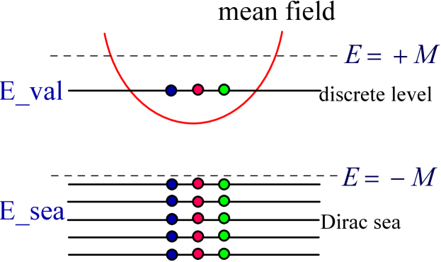
Figure 1: A schematic view of baryons in the Relativistic Mean Field Approximation. There are three “valence” quarks at a discrete energy level created by the mean field, and the negative-energy Dirac continuum distorted by the mean field, as compared to the free one.

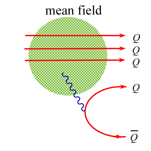
Figure 2: Equivalent view of baryons in the same approximation, where the distorted Dirac sea is presented as $Q\bar{Q}$ pairs. The average number of $Q\bar{Q}$ pairs is proportional to the amplitude squared of the mean field, times $N_{c}$.

The correct lowest baryons’ quantum numbers arise as a result of the quantization of the rotation of the mean chiral field in the ordinary and in the flavor spaces Witten . If the mean chiral field is presented as a unitary $3\times 3$ matrix $V(\vec{x})$, the rotated field is

$$U(\vec{x})=R\,V(\vec{x})\,R^{\dagger}$$ (1)

where $R$ is an $SU(3)$ rotation matrix; it can be parameterized by eight “Euler angles” as it is done, for example, in Appendix A. We shall for simplicity set the strange quark mass $m_{s}=0$; in this limit any rotated mean field (1) is, classically, as good as the un-rotated one: the baryon energy is degenerate in rotations.

In quantum mechanics, however, the rotations are quantized. As first pointed out by Witten Witten and then derived using different techniques by a number of authors quantization , the quantization rule is such that the lowest baryon multiplets are the octet with spin 1/2 and the decuplet with spin 3/2 (i.e. exactly those observed in nature) followed by the exotic anti-decuplet with spin 1/2 again. The parity of all rotational states is the same. Those baryons are distinguished by the rotational wave functions depending on the eight Euler angles parameterizing the $SU(3)$ rotation matrix $R$; the wave functions are given explicitly in Section IV.

Qualitatively, one can think of different baryons as “living” in different parts of an 8-dimensional globe parametrized by 8 “Euler angles”. The $\Theta^{+}$ lives near the North pole of that globe, at least in the academic limit of large $N_{c}$. The average polar angle for the rotational state corresponding to the $\Theta^{+}$ vanishes as $1/\sqrt{N_{c}}$, see section IV.D. Therefore, in the limit $N_{c}\to\infty$ one can approximate the rotation by small (kaon) fluctuations about the North pole. Mathematically, it comes to the Callan–Klebanov “bound-state approach to strangeness” CK where one studies the linear response of a nucleon to a small-amplitude kaon perturbation, or the $KN$ scattering, to see if there is a $\Theta^{+}$ resonance. In such approach the narrow $\Theta^{+}$ does not exist, at least in the Skyrme model for the $KN$ scattering, unless one extends the parameters of the model KlebanovRho . The Skyrme model for the self-consistent chiral field is, however, not realistic, and it is unclear what lesson can one draw from the existence or non-existence of a resonance in this particular dynamical model.

Even more important, it is exactly the situation where the large $N_{c}$ limit can hardly be trusted. In reality at $N_{c}=3$ the $\Theta^{+}$ rotational wave function is spread over the whole 8-dimensional globe and is far from the “North pole”. A quantum-mechanical model of the situation has been suggested by Cohen Cohen03 and Pobylitsa Pobylitsa03 ; the model can be solved numerically at any $N_{c}$ Cohen04 . It turns out that the energy levels at $N_{c}=3$ differ radically from their positions at $N_{c}\to\infty$. Given this experience, we shall treat the $\Theta^{+}$ rotational wave function exactly at $N_{c}=3$, see section IV. At the same time we shall neglect the fluctuations of the chiral field about its mean field value since these are suppressed additionally as are any generic loop corrections.

In this approach, all low-energy properties of baryons from the $\left({\bf 8},{\textstyle{\frac{1}{2}}}^{+}\right)$, $\left({\bf 10},\frac{3}{2}^{+}\right)$and $\left({\bf\overline{10}},{\textstyle{\frac{1}{2}}}^{+}\right)$multiplets (including e.g. parton distributions at low virtuality) follow from the shape of the mean chiral field in the common or ‘classical’ baryon; the difference and splitting between baryons from those multiplets arise exclusively from the difference in their rotational wave functions. This difference can be immediately translated into the quark wave functions of the individual baryons, both in the infinite momentum PP-IMF ; DP-Fock and the rest D04-Minn frames. In Section III we present a compact general formalism how to find the 3-quark, 5-quark, 7-quark … wave functions inside the octet, decuplet and antidecuplet baryons, which is further detailed in Sections V and VI. In Section VII we find the quark wave functions of the $3Q$ components in the octet and decuplet baryons. In the non-relativistic limit (implying a weak mean field), we obtain the old $SU(6)$ quark wave functions for the octet and decuplet baryons but with well-defined relativistic corrections. The $5Q$ wave functions in the ordinary and exotic baryons can be also found explicitly D04-Minn ; DP-Fock , see Section VIII.

In Sections IX–XI we develop a formalism how to compute observables related to the 3- and 5-quark Fock components of baryons, and apply it in Section XII to estimate the nucleon axial constant and the transition matrix element of the strange axial current between the $\Theta^{+}$ and the nucleon: it gives an estimate of the $\Theta^{+}\to KN$ decay width. The latter turns out to be very small, 2-4 MeV, although with a large uncertainty discussed in Section XIII.

The essence of QCD with its spontaneous breaking of chiral symmetry is that adding a low-energy pseudoscalar meson (or a $\bar{Q}Q$ pair) to a baryon is equivalent to rotating the vacuum state along the Goldstone valley, meaning no change of the physical state. In order to separate the true $\bar{Q}Q$ pairs in a baryon from those in the vacuum, one has to consider baryons in the Infinite Momentum Frame (IMF). In this and only this frame the true $\bar{Q}Q$ pairs in a baryon have an infinite momentum as contrasted to those in the vacuum, which have a finite momentum. Therefore, an accurate definition of what are the 3-, 5-,… Fock components of baryons can be made only in the IMF. It also has the advantage that the vector and axial currents with a finite momentum transfer do not create or annihilate quarks with infinite momenta. The baryon matrix elements are thus non-zero only between Fock components with equal number of quarks and antiquarks.

Since the $\Theta^{+}$ has no $3Q$ component it means that one has to calculate the matrix element between the $5Q$ component of the $\Theta^{+}$ and the $5Q$ component of the nucleon. In principle, one has to add also the $7Q\to 7Q,\,9Q\to 9Q...$ transitions, but we neglect them in the present paper. To control this approximation, we compute, using the same technique, the nucleon axial constant $g_{A}(N)$. In the (very crude) non-relativistic $3Q$ approximation to nucleons, this constant is approximately $5/3=1.667$; taking into account the $5Q$ component of the nucleon moves it to the value of $1.36$ being already not too far from the experimental value $g_{A}(N)=1.27$ PDG . It should be noted that the summation of the contributions of any number of $\bar{Q}Q$ pairs in the Relativistic Mean Field Approximation to nucleons moves $g_{A}(N)$ quite close to the experimental value corrNc1 . In the $5Q$ approximation to the $\Theta^{+}\to KN$ transition, we obtain $g_{A}(\Theta\to KN)\approx 0.14-0.2$ leading to the estimate $\Gamma_{\Theta}\approx 2-4\,{\rm MeV}$. In this estimate, we neglect the quark exchange contributions to the $\Theta^{+}\to KN$ transition, which are potentially capable of reducing further the width. Qualitatively, the axial constant of the $\Theta^{+}\to KN$ transition is small because it is analogous not to the large nucleon axial constant itself but to the change of this constant as one goes from the $3Q$ to the $5Q$ contribution.

II The effective action

The effective action approximating QCD at low momenta describes “constituent” quarks with the momentum dependent dynamical mass $M(p)$ interacting with the scalar ($\Sigma$) and pseudoscalar (${\bf\Pi}$) fields such that $\Sigma^{2}+{\bf\Pi}^{2}=1$ at spatial infinity. The momentum dependence $M(p)$ serves as a formfactor of the constituent quarks and provides the effective theory with the ultraviolet cutoff. Simultaneously, it makes the theory non-local. The action is DP86

$$\!S_{\rm eff}\!=\!\!\int\!\frac{d^{4}pd^{4}p^{\prime}}{(2\pi)^{8}}\,\bar{\psi}(p)\left[p\hskip-5.0pt/\,(2\pi)^{4}\delta^{(4)}(p-p^{\prime})\!-\!\sqrt{M(p)}\left(\Sigma(p\!-\!p^{\prime})+i\Pi(p\!-\!p^{\prime})\gamma_{5}\right)\sqrt{M(p^{\prime})}\right]\psi(p^{\prime}),$$ (2)

where $\psi,\bar{\psi}$ are quark fields carrying color, flavor and Dirac bispinor indices. In the instanton model of the QCD vacuum from where this action has been originally derived the function $M(p)$ is such that there is no real solution of the mass-shell equation $p^{2}=M(-p^{2})$, therefore quarks are not observable as asymptotic states, – only their bound states. However, this is not the true confinement. Unfortunately, the instanton model’s $M(p)$ has a cut at $p^{2}=0$ corresponding to massless gluons left in that model. In the true confining theory there should be no such cuts. Nevertheless, such $M(p)$ creates some kind of a soft “bag” for quarks. Contrary to the naive bag picture which does not respect relativistic invariance, eq. (2) supports all general principles and sum rules for conserved quantities.

The scalar, pseudoscalar DP-preprint , vector and axial Bron-Dor mesons follow from the correlation functions computed from eq. (2). The light-cone quark wave functions of the pion and of the photon have been found in Ref. PPRWG ; the electromagnetic pion radius has been computed in the original paper DP86 .

Turning to baryons, the mean $\Sigma,\Pi$ field (called chiral field for short in what follows) in the full non-local formulation (2) has been found by Broniowski, Golli and Ripka BGR . It sets an example how one has to proceed in the model calculations. However, to simplify the mathematics we shall use here a more standard approach: we shall replace the constituent quark mass by a constant $M=M(0)$ and mimic the decreasing function $M(p)$ by the UV Pauli–Villars cutoff SF .

III Baryon wave function in terms of quark creation-annihilation operators

Let $a,a^{\dagger}({\bf p})$ and $b,b^{\dagger}({\bf p})$ be the annihilation–creation operators of quarks and antiquarks (respectively) of mass $M$, satisfying the usual anticommutator algebra $\{a({\bf p})a^{\dagger}({\bf p^{\prime}})\}=\{b({\bf p})b^{\dagger}({\bf p^{\prime}})\}=(2\pi)^{3}\delta^{(3)}({\bf p}-{\bf p^{\prime}})$ and annihilating the vacuum state $a,b|0\!\!>=\!0$, $<\!\!0|a^{\dagger},b^{\dagger}\!=\!0$. For quarks, the annihilation-creation operators carry, apart from the 3-momentum ${\bf p}$, also the color $\alpha$, flavor $f$ and spin $\sigma$ indices but we shall suppress them until they are explicitly needed. The Dirac sea is presented by the coherent exponent of the quark and antiquark creation operators PP-IMF ,

$${\rm coherent\;exponent\;for}\;\bar{Q}Q\;{\rm pairs}=\exp\left(\int\!(d{\bf p})(d{\bf p^{\prime}})\,a^{\dagger}({\bf p})\,W({\bf p},{\bf p^{\prime}})\,b^{\dagger}({\bf p^{\prime}})\right)|0\!>,$$ (3)

where $(d{\bf p})=d^{3}{\bf p}/(2\pi)^{3}$ and $W({\bf p_{1}},{\bf p_{2}})$ is the quark Green function at equal times in the background $\Sigma,{\bf\Pi}$ fields PP-IMF ; DP-Fock (see Fig. 2); we shall specify the function $W$ below. In the mean field approximation the chiral field is replaced by the spherically-symmetric self-consistent field:

$$\pi({\bf x})={\bf n\cdot\tau}P(r),\qquad{\bf n}={\bf x}/r,\qquad\Sigma({\bf x})=\Sigma(r).$$ (4)

On the chiral circle (to which we restrict ourselves for simplicity) $\Pi={\bf n\cdot\tau}\,\sin P(r),\;\Sigma(r)=\cos P(r)$ where $P(r)$ is the profile function of the self-consistent field. It is fairly approximated by DP-CQSM ; DPPrasz

$$P(r)=2\,{\rm atan}\left(\frac{r_{0}^{2}}{r^{2}}\right),\qquad r_{0}\approx\frac{0.8}{M},$$ (5)

where $M\approx 345\,{\rm MeV}$ is the dynamical quark mass at zero virtuality, known to fit numerous observables within the instanton mechanism of the spontaneous chiral symmetry breaking DP86 .

The self-consistent chiral field (5) creates a bound-state level for quarks, whose wave function $\psi_{\rm lev}$ satisfies the static Dirac equation with eigenenergy $E_{\rm lev}$ KR ; BB ; DP-CQSM :

$$\psi_{\rm lev}({\bf x})=\left(\begin{array}[]{c}\epsilon^{ji}h(r)\\ -i\epsilon^{jk}\,({\bf\sigma\!\cdot\!n})^{i}_{k}\,j(r)\end{array}\right),\qquad\left\{\begin{array}[]{c}h^{\prime}+h\,M\sin P-j(M\cos P+E_{\rm lev})=0,\\ j^{\prime}+2j/r-j\,M\sin P-h(M\cos P-E_{\rm lev})=0,\end{array}\right.$$ (6)

where $i=1,2$ is the spin and $j=1,2=u,d$ is the isospin index. In the non-relativistic limit ($E_{\rm lev}\approx M$) the $L\!=\!0$ upper component of the Dirac bispinor $h(r)$ is large while the $L\!=\!1$ lower component $j(r)$ is small. Solving eq. (6) for the self-consistent field (5) one finds that ‘valence’ quarks are tightly bound ($E_{\rm lev}=200\,{\rm MeV}$) but the lower component $j(r)$ is still substantially smaller than the upper one $h(r)$, see Figs. 3,4.

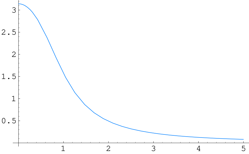
Figure 3: The space profile of the self-consistent chiral field $P(r)$ in light baryons. One unit on the horizontal axis is $r_{0}=0.8/M=0.46\,{\rm fm}$.

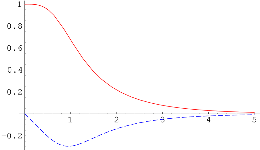
Figure 4: Bound-state quark upper $s$-wave component $h(r)$ (solid) and the lower $p$-wave component $j(r)$ (dashed) in light baryons. The three valence quarks have the energy $E_{\rm lev}=200\,{\rm MeV}$ each.

The valence quark part of the baryon wave function is given by the product of $N_{c}$ quark creation operators that fill in the discrete level PP-IMF :

$${\rm valence\;quarks\;wave\;function} = \prod_{{\rm color}=1}^{N_{c}}\int(d{\bf p})\,F({\bf p})\,a^{\dagger}({\bf p}),$$ (7)

$$F({\bf p}) = \int\!(d{\bf p^{\prime}})\sqrt{\frac{M}{\epsilon_{p}}}\!\left[\bar{u}({\bf p})\,\gamma_{0}\,\psi_{\rm lev}({\bf p})\,(2\pi)^{3}\delta({\bf p}\!-\!{\bf p^{\prime}})\!-\!W({\bf p},{\bf p^{\prime}})\,\bar{v}({\bf p^{\prime}})\,\gamma_{0}\,\psi_{\rm lev}(-\!{\bf p^{\prime}})\right]\!,$$ (8)

where $\psi_{\rm lev}({\bf p})$ is the Fourier transform of eq. (6). The second term in Eq. (8) is the contribution of the distorted Dirac sea to the one-quark wave function. $u_{\sigma}({\bf p})$ and $v_{\sigma}({\bf p})$ are the plane-wave Dirac bispinors projecting to the positive and negative frequencies, respectively. In the standard basis they have the form

$$u_{\sigma}({\bf p})=\left(\begin{array}[]{c}\sqrt{\frac{\epsilon+M}{2M}}s_{\sigma}\\ \sqrt{\frac{\epsilon-M}{2M}}\frac{{\bf p\cdot\sigma}}{|p|}s_{\sigma}\end{array}\right),\qquad v_{\sigma}({\bf p})=\left(\begin{array}[]{c}\sqrt{\frac{\epsilon-M}{2M}}\frac{{\bf p\cdot\sigma}}{|p|}s_{\sigma}\\ \sqrt{\frac{\epsilon+M}{2M}}s_{\sigma}\end{array}\right),\qquad\bar{u}u=1=-\bar{v}v\,,$$ (9)

where $\epsilon=\!+\!\sqrt{{\bf p}^{2}+M^{2}}$ and $s_{\sigma}$ are two 2-component spinors normalized to unity, for example,

$$s_{1}=\left(\begin{array}[]{c}1\\ 0\end{array}\right),\qquad s_{2}=\left(\begin{array}[]{c}0\\ 1\end{array}\right),\qquad\sigma=1,2.$$ (10)

The full baryon wave function is given by the product of the valence part (7) and the coherent exponent (3) describing the distorted Dirac sea. Symbolically, one writes the baryon wave function in terms of the quark and antiquark creation operators  PP-IMF :

$$B[a^{\dagger},b^{\dagger}]=\prod_{{\rm color}=1}^{N_{c}}\int(d{\bf p})\,F({\bf p})\,a^{\dagger}({\bf p})\;\exp\left(\int\!(d{\bf p})(d{\bf p^{\prime}})\,a^{\dagger}({\bf p})\;W({\bf p},{\bf p^{\prime}})\,b^{\dagger}({\bf p^{\prime}})\right)|0\!>.$$ (11)

At this point one has to recall that the saddle point at the self-consistent chiral field is degenerate in global translations and global $SU(3)$ flavor rotations (1) (the $SU(3)$ breaking by the strange mass can be treated as a perturbation later). Integrating over translations leads to the momentum conservation: the sum of all quarks and antiquarks momenta have to be equal to the baryon momentum. Integration over rotations $R$ leads to the projection of the flavor state of all quarks and antiquarks onto the spin-flavor state $B(R)$ describing a particular baryon from the $\left({\bf 8},\frac{1}{2}^{+}\right),\left({\bf 10},\frac{3}{2}^{+}\right)$ or $\left({\bf\overline{10}},\frac{1}{2}^{+}\right)$ multiplet.

Restoring color ($\alpha=1,2,3$), flavor ($f=1,2,3$), isospin ($j=1,2$) and spin ($\sigma=1,2$) indices, the quark wave function inside a particular baryon $B$ with spin projection $k$ is given, in full glory, by PP-IMF ; DP-Fock

$$\Psi_{k}(B) = \int\!dR\,B^{*}_{k}(R)\,\epsilon^{\alpha_{1}\alpha_{2}\alpha_{3}}\prod_{n=1}^{3}\int\!(d{\bf p_{n}})\,R^{f_{n}}_{j_{n}}\,F^{j_{n}\sigma_{n}}({\bf p_{n}})\,a^{\dagger}_{\alpha_{n}f_{n}\sigma_{n}}({\bf p_{n}})$$ (12)

$$\cdot \exp\left(\int\!(d{\bf p})(d{\bf p^{\prime}})\,a^{\dagger}_{\alpha f\sigma}({\bf p})\,R^{f}_{j}\,W^{j\sigma}_{j^{\prime}\sigma^{\prime}}({\bf p},{\bf p^{\prime}})\,R^{\dagger\,j^{\prime}}_{f^{\prime}}\,b^{\dagger\,\alpha f^{\prime}\sigma^{\prime}}({\bf p^{\prime}})\right)|0\!\!>\,.$$

Acting on the vacuum state $|0\!>$ the operators $a^{\dagger}$ create three ‘valence’ quarks at the bound-state discrete level with the wave function $F$, while the $a^{\dagger},b^{\dagger}$ operators in the exponent create any number of additional quark-antiquark pairs whose wave function is $W$. Eq. (12) is thus a full relativistic field-theoretic description of baryons, involving an infinite number of degrees of freedom.

Note that the three ‘valence’ quarks are antisymmetric in color whereas the additional $\bar{Q}Q$ pairs appear in color singlets. The spin-flavor quark structure of a particular baryon arises from projecting a general $QQQ+n\bar{Q}Q$ state onto the quantum numbers of the baryon in question; this is achieved by means of integrating over all spin-flavor rotations $R$ with the rotational wave function $B^{*}_{k}(R)$ unique for a given baryon.

The third row of the matrix $R^{f}_{j},\,f=3,$ introduces strange quarks both at the valence level and in the sea; hence hyperons with explicit strangeness will, generally, have valence $s$ quarks, and non-strange baryons will contain $\bar{s}s$ pairs, even though only the $u,d$ quarks are affected by the chiral field (4), which is reflected by the fact that the valence-level wave function $F$ and the pair wave function $W$ have not full $SU(3)$ but only isospin indices $j=1,2=u,d$.

Eq. (12) encodes an enormous amount of information as it is the generating functional for the quark wave functions in all Fock components of baryons from the lowest multiplets. Expanding the coherent exponent to the 0^th, 1^st, 2^nd… order one reads off the 3-, 5-, 7-… quark wave functions of a particular baryon from the octet, decuplet or antidecuplet. All this information can be put in a compact form because the Relativistic Mean Field Approximation is being used.

To make this powerful formula fully workable, we need to give explicit expressions for the baryon rotational wave functions $B(R)$, the valence wave function $F^{j\sigma}({\bf p})$ and the $\bar{Q}Q$ wave function in a baryon $W^{j\sigma}_{j^{\prime}\sigma^{\prime}}({\bf p},{\bf p^{\prime}})$.

IV Baryon rotational wave functions

In general, baryon rotational states $B(R)$ are given by the $SU(3)$ Wigner finite-rotation matrices hyperons , and any particular projection can be obtained by a routine $SU(3)$ Clebsch–Gordan technique. However, in order to see the symmetries of the quark wave functions it is helpful to use explicit expressions for $B(R)$, and integrate over the Haar measure in eq. (12) explicitly.

We list below the rotational D-functions for the multiplets $\left({\bf 8},\frac{1}{2}\right)$, $\left({\bf 10},\frac{3}{2}\right)$ and $\left({\bf\overline{10}},\frac{1}{2}\right)$ in terms of the product of the $R$ matrices. Since the projecting onto a specific baryon in eq. (12) involves its conjugate rotational wave function, we list the conjugate functions only. The un-conjugate ones are obtained by hermitian conjugation.

IV.1 $\left({\bf 8},\frac{1}{2}\right)$

From the $SU(3)$ group point of view, the octet of baryons transforms exactly as an octet of mesons; therefore, its rotational wave function can be composed of a quark (transforming as $R$) and an antiquark (transforming as $R^{\dagger}$). Accordingly, the rotational wave function of an octet baryon labeled by $a=1\ldots 8$ and having a spin index $k=1,2$ is

$$\left[D^{(8,\frac{1}{2})\,*}(R)\right]^{a}_{k}\sim\,\epsilon_{kl}\,R^{\dagger\,l}_{f}\left(t^{a}\right)^{f}_{g}\,R^{g}_{3}.$$ (13)

where $\epsilon_{kl}$ is the antisymmetric $2\!\times\!2$ tensor and $t^{a}$ are the $SU(3)$ generators. In particular, the proton ($a=6+i7$) and neutron ($a=4+i5$) rotational wave functions with spin $k=1,2$ are

$$p_{k}(R)^{*}=\sqrt{8}\,\epsilon_{kl}\,R^{\dagger\,l}_{1}\,R^{3}_{3},\qquad n_{k}(R)^{*}=\sqrt{8}\,\epsilon_{kl}\,R^{\dagger\,l}_{2}\,R^{3}_{3}.$$ (14)

IV.2 $\left({\bf 10},\frac{3}{2}\right)$

The decuplet states can be composed of three quarks; they are labeled by a triple flavor index $\{f_{1}f_{2}f_{3}\}$ symmetrized in flavor and by a triple spin index $\{k_{1}k_{2}k_{3}\}$ symmetrized in spin:

$$\left[D^{(10,\frac{3}{2})\,*}(R)\right]_{\{f_{1}f_{2}f_{3}\},\{k_{1}k_{2}k_{3}\}}\sim\epsilon_{k^{\prime}_{1}k_{1}}\epsilon_{k^{\prime}_{2}k_{2}}\epsilon_{k^{\prime}_{3}k_{3}}\,\left.R_{f_{1}}^{\dagger\,k^{\prime}_{1}}\,R_{f_{2}}^{\dagger\,k^{\prime}_{2}}\,R_{f_{3}}^{\dagger\,k^{\prime}_{3}}\right|_{{\rm sym\;in}\;\{f_{1}f_{2}f_{3}\}}\,.$$ (15)

For example, the $\Delta$-resonance rotational wave functions are

$$\Delta^{++},\;{\rm spin\;projection}\;+\!\frac{3}{2} : \qquad\Delta^{++}_{\uparrow\uparrow}(R)^{*}=\sqrt{10}\,R^{\dagger\,2}_{1}R^{\dagger\,2}_{1}R^{\dagger\,2}_{1},$$ (16)

$$\Delta^{0},\,{\rm spin\;projection}\,+\!\frac{1}{2} : \qquad\Delta^{0}_{\uparrow}(R)^{*}=\sqrt{10}\,R^{\dagger\,2}_{2}(2R^{\dagger\,2}_{1}R^{\dagger\,1}_{2}\!+\!R^{\dagger\,2}_{2}R^{\dagger\,1}_{1})\,.$$ (17)

IV.3 $\left({\bf\overline{10}},\frac{1}{2}\right)$

From the $SU(3)$ group point of view, the antidecuplet can be composed of three antiquarks and its conjugate rotational wave function is

$$\left[D^{(\overline{10},\frac{1}{2})\,*}(R)\right]_{k}^{\{f_{1}f_{2}f_{3}\}}\sim\left.R^{f_{1}}_{3}\,R^{f_{2}}_{3}\,R^{f_{3}}_{k}\right|_{{\rm sym\;in}\;\{f_{1}f_{2}f_{3}\}}.$$ (18)

In particular,

$$\Theta^{+},\;{\rm spin\;projection}\;k : \qquad\Theta_{k}(R)^{*}=\sqrt{30}\,R^{3}_{3}R^{3}_{3}R^{3}_{k}\,,$$ (19)

$${\rm neutron}^{*}\;{\rm from}\;\overline{10}\;,\;{\rm spin\;projection}\;k : \qquad n^{\overline{10}}_{k}(R)^{*}=\sqrt{10}\,(2R^{2}_{3}R^{3}_{3}R^{3}_{k}+R^{3}_{3}R^{3}_{3}R^{2}_{k})\,.$$ (20)

All the rotational wave functions above are normalized in such a way that for any (but the same) spin projection

$$\int\!dR\,B^{*}_{\rm spin}(R)\,B^{\rm spin}(R)=1;$$ (21)

for different spin projections the integral is zero. Rotational wave functions belonging to different baryons are also orthogonal. It can be easily checked directly using the concrete parametrization of the $SU(3)$ rotation matrices $R$ from Appendix A and performing the 8-dimensional integration with the measure defined there.

IV.4 Large $N_{c}$ limit

If $N_{c}$ is not equal to three but is treated as a free parameter, the lightest baryons are not the octet, decuplet and antidecuplet but some large $SU(3)$ multiplets whose dimensions depend on $N_{c}$. What $SU(3)$ multiplets are the large-$N_{c}$ prototypes of the usual multiplets at $N_{c}\!=\!3$, is not uniquely defined. It seems natural to define the prototype multiplets in such a way that their lightest members are “nucleons” with spin and isospin ${\textstyle{\frac{1}{2}}}$, “$\Delta$’s” with spin and isospin $\frac{3}{2}$, and “$\Theta$” with spin ${\textstyle{\frac{1}{2}}}$ and isospin 0: this prescription is sufficient to define unambiguously the large-$N_{c}$ prototypes of the octet, decuplet and antidecuplet DuPrasz ; Cohen03 ; DP-03 .

The rotational wave functions of the large-$N_{c}$ analogs of the $N$, $\Delta$ and $\Theta$ are obtained from eqs.(14,16) and (19) by multiplying the corresponding equations by a factor $\left(R^{3}_{3}\right)^{N_{c}-3}$. In Appendix A we give a concrete example of the parametrization of a general $SU(3)$ rotation matrix $R$ in terms of eight “Euler” angles. In fact they parameterize the $S^{3}\times S^{5}$ space, – the direct product of the $3d$ and $5d$ spheres. In this parametrization,

$$R^{3}_{3}=e^{i\alpha_{21}}\,\cos\phi_{2}\,\cos\theta,\qquad\theta,\phi_{2}\in\left(0,\frac{\pi}{2}\right),$$ (22)

where $\theta$ and $\phi_{2}$ can be viewed as polar angles of the $5d$ sphere. It is clear that at $N_{c}\to\infty$ the rotational wave functions of the “$N$”, “$\Delta$” and “$\Theta$” are squeezed near the “North pole” of the sphere $S^{5}$ since the average polar angles vanish as $\theta,\phi_{2}\sim 1/\sqrt{N_{c}}$. The rotated self-consistent field (1) can be also parameterized à la Callan–Klebanov CK :

$$U=RVR^{\dagger}=\sqrt{V}U_{K}\sqrt{V},\qquad V({\bf x})=\left(\begin{array}[]{cc}\exp\left[i(\mbox{\boldmath{$n$}}\cdot\mbox{\boldmath{$\tau$}})P(r)\right]&\begin{array}[]{c}0\\ 0\end{array}\\ \begin{array}[]{cc}0&0\end{array}&1\end{array}\right),$$ (23)

where the meson $SU(3)$ unitary matrix $U_{K}$ is, for small meson fluctuations $\phi$ about the self-consistent field $V$,

$$U_{K}=1_{3}+i\phi^{A}\lambda^{A},\qquad A=1...8,$$ (24)

$$\pi^{\pm}=\frac{\phi^{1}\pm i\phi^{2}}{\sqrt{2}},\quad\pi^{0}=\phi^{3},\quad K^{+}=\frac{\phi^{4}+i\phi^{5}}{\sqrt{2}},\quad K^{0}=\frac{\phi^{6}+i\phi^{7}}{\sqrt{2}},\quad\eta=\phi^{8}.$$ (25)

One can compare both sides of eq. (23) and find the meson fields in baryons corresponding to rotations. In particular, for rotations “near the North pole” i.e. at small angles $\theta,\phi_{2}$, one finds the kaon field

$$K^{+}=-\sqrt{2}\,\sin\frac{P(r)}{2}\left[\theta n_{z}+\phi_{2}(n_{x}-in_{y})\right],\qquad K^{0}=-\sqrt{2}\,\sin\frac{P(r)}{2}\left[\theta(n_{x}+in_{y})-\phi_{2}n_{z}\right],$$ (26)

meaning that at large $N_{c}$ the amplitude of the kaon fluctuations in the prototype baryons “$N$”, “$\Delta$” and “$\Theta$” is vanishing as $\sim 1/\sqrt{N_{c}}$. Therefore, the $\Theta$ problem becomes that of the linear response of a nucleon to a small kaon fluctuation, and can be studied in a particular model for the effective chiral lagrangian KlebanovRho . However, in reality at $N_{c}\!=\!3$ the rotational wave functions of $N$ (14), $\Delta$ (16) and $\Theta$ (19) correspond to large angles $\theta,\phi_{2}$ and are not concentrated near the “North pole”. It means that the kaon field in these baryons is generally not small. Therefore, in what follows we shall use the exact $N_{c}\!=\!3$ rotational wave functions (14,16,19).

V $\bar{Q}Q$ pair wave function

As explained in Refs. PP-IMF ; DP-Fock , the pair wave function $W^{j\sigma}_{j^{\prime}\sigma^{\prime}}({\bf p},{\bf p^{\prime}})$ is expressed through the finite-time quark Green function at equal times in the external static chiral field (4); schematically, it is shown in Fig. 2. We shall need the Fourier transforms of the self-consistent chiral field,

$$\qquad\Pi({\bf q})^{j}_{j^{\prime}}=\int\!d^{3}{\bf x}\,e^{-i{\bf q\cdot x}}\,({\bf n}\cdot\tau)^{j}_{j^{\prime}}\,\sin P(r),\qquad\Sigma({\bf q})^{j}_{j^{\prime}}=\int\!d^{3}{\bf x}\,e^{-i{\bf q\cdot x}}\,(\cos P(r)-1)\delta^{j}_{j^{\prime}},$$ (27)

where $\Pi({\bf q})$ is purely imaginary and odd while $\Sigma({\bf q})$ is real and even.

In Refs. PP-IMF ; DP-Fock a simplified interpolating approximation for the pair wave function $W$ has been derived, which becomes exact in three limiting cases: i) small pion field $P(r)$, ii) slowly varying $P(r)$, iii) fast varying $P(r)$. In the infinite momentum frame the result is a function of the fractions of the baryon’s longitudinal momenta carried by the quark ($z$) and antiquark ($z^{\prime}$) of the pair, and their transverse momenta ${\bf p}_{\perp},{\bf p^{\prime}}_{\perp}$ footnote1 :

$$W^{j\sigma}_{j^{\prime}\sigma^{\prime}}(z,{\bf p}_{\perp};z^{\prime},{\bf p^{\prime}}_{\perp}) = \frac{M{\cal M}}{2\pi Z}\,\left\{\Sigma^{j}_{j^{\prime}}({\bf q})\left[M(z^{\prime}-z)\tau_{3}+(z{\bf p^{\prime}}-z^{\prime}{\bf p})_{\perp}\cdot\tau_{\perp}\right]^{\sigma}_{\sigma^{\prime}}\right.$$ (28)

$$+ \left.i\,\Pi^{j}_{j^{\prime}}({\bf q})\left[-M(z^{\prime}+z){\bf 1}+i\epsilon_{\alpha\beta}(z{\bf p^{\prime}}-z^{\prime}{\bf p})_{\perp\alpha}\tau_{\perp\beta}\right]^{\sigma}_{\sigma^{\prime}}\right\},$$

$$Z = {\cal M}^{2}zz^{\prime}(z+z^{\prime})+z(p^{{}^{\prime}2}_{\perp}+M^{2})+z^{\prime}(p^{2}_{\perp}+M^{2}),\qquad{\bf q}=\left(({\bf p}+{\bf p^{\prime}})_{\perp},(z+z^{\prime}){\cal M}\right).$$

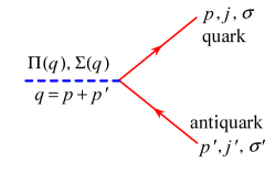
Figure 5: The $\bar{Q}Q$ pair wave function in a baryon in the Relativistic Mean Field Approximation is related to the Fourier transform of the static self-consistent chiral field.

Here $j,j^{\prime}=1,2$ are the isospin and $\sigma,\sigma^{\prime}=1,2$ are the spin projections, $\tau_{1,2,3}$ are Pauli matrices, $\epsilon_{\alpha\beta}$ is the antisymmetric $2d$ tensor, the primed indices refer to the antiquark; ${\cal M}$ is the baryon and $M$ is the constituent quark masses, ${\bf q}$ is the 3-momentum of the pair as a whole, transferred from the background field $\Sigma({\bf q}),\Pi({\bf q})$.

The pair wave function $W$ is normalized in such a way that the creation-annihilation operators in eq. (12) satisfy the anticommutation relations

$$\{a^{\alpha_{1}f_{1}\sigma_{1}}(z_{1},{\bf p}_{1\perp}),a^{\dagger}_{\alpha_{2}f_{2}\sigma_{2}}(z_{2},{\bf p}_{2\perp})\}=\delta^{\alpha_{1}}_{\alpha_{2}}\delta^{f_{1}}_{f_{2}}\delta^{\sigma_{1}}_{\sigma_{2}}\,\delta(z_{1}-z_{2})\,(2\pi)^{2}\delta^{(2)}({\bf p}_{1\perp}-{\bf p}_{2\perp})$$ (29)

and similarly for $b,b^{\dagger}$, and the integrals over momenta there are understood as $\int\!dz\!\int d^{2}{\bf p}_{\perp}/(2\pi)^{2}$.

The pair wave function can be written in a more compact form by introducing the fraction of the longitudinal momentum of the pair carried by the antiquark $y$, and the transverse combination ${\bf Q_{\perp}}$,

$$y=\frac{z^{\prime}}{z+z^{\prime}},\qquad q_{z}=\frac{z+z^{\prime}}{{\cal M}},\qquad{\bf Q}_{\perp}=\frac{z{\bf p^{\prime}}_{\perp}-z^{\prime}{\bf p}_{\perp}}{z+z^{\prime}}\,.$$ (30)

With this substitution eq. (28) takes the form

$$W^{j\sigma}_{j^{\prime}\sigma^{\prime}}(y,{\bf q},{\bf Q}_{\perp})=\frac{M{\cal M}}{2\pi}\,\frac{\Sigma^{j}_{j^{\prime}}({\bf q})\left[M(2y-1)\tau_{3}+{\bf Q}_{\perp}\cdot\tau_{\perp}\right]^{\sigma}_{\sigma^{\prime}}+i\,\Pi^{j}_{j^{\prime}}({\bf q})\left[-M{\bf 1}+i\epsilon_{\alpha\beta}{\bf Q}_{\perp\alpha}\tau_{\perp\beta}\right]^{\sigma}_{\sigma^{\prime}}}{{\bf Q}_{\perp}^{2}+M^{2}+y(1-y){\bf q}^{2}}\,.$$ (31)

VI Bound-state wave function

As seen from eq. (8), the discrete-level wave function $F^{j\sigma}({\bf p})=F^{j\sigma}_{\rm lev}({\bf p})+F^{j\sigma}_{\rm sea}({\bf p})$ consists of two pieces: one is directly the wave function of the valence level, the other is related to the change of the number of quarks at the discrete level as due to the presence of the Dirac sea; it is a relativistic effect and can be ignored in the non-relativistic limit, together with the lower $L\!=\!1$ component $j(r)$ of the level wave function. Indeed, in the baryon rest frame the evaluation of the first term in eq. (8) gives

$$F^{j\sigma}_{\rm lev}({\bf p})=\epsilon^{j\sigma}\left(\sqrt{\frac{E_{\rm lev}+M}{2E_{\rm lev}}}h(p)+\sqrt{\frac{E_{\rm lev}-M}{2E_{\rm lev}}}j(p)\right),$$ (32)

where $h(p),j(p)$ are the Fourier transforms of the valence wave functions (6):

$$h(p) = \int\!d^{3}x\,e^{-i{\bf p}\cdot{\bf x}}\,h(r)=4\pi\int\!dr\,r^{2}\frac{\sin\,pr}{pr}\,h(r),$$ (33)

$$j^{a}(p) = \int\!d^{3}x\,e^{-i{\bf p}\cdot{\bf x}}\,(-in^{a})j(r)=\frac{p^{a}}{|p|}j(p),\qquad j(p)=\frac{4\pi}{p^{2}}\!\int\!dr\,(pr\,\cos\,pr-\sin\,pr)\,j(r).$$ (34)

One sees that the second term in eq. (32) is double-suppressed in the non-relativistic limit $E_{\rm lev}\approx M$: first, owing to the kinematical factor, second, since in this limit the $L\!=\!1$ wave $j(r)$ is much less than the $L\!=\!0$ wave $h(r)$.

In the infinite momentum frame the evaluation of the bispinors $\bar{u},\bar{v}$ from eq. (9) produces PP-IMF ; DP-Fock

$$F^{j\sigma}_{\rm lev}(z,p_{\perp})=\sqrt{\frac{{\cal M}}{2\pi}}\left[\epsilon^{j\sigma}h(p)+\left(p_{z}{\bf 1}+i\epsilon_{\alpha\beta}p_{\perp\alpha}\tau_{\perp\beta}\right)^{\sigma}_{\sigma^{\prime}}\epsilon^{j\sigma^{\prime}}\frac{j(p)}{|p|}\right]_{p_{z}=z{\cal M}-E_{\rm lev}}$$ (35)

Similarly, the evaluation of the “sea” part of the discrete-level wave function gives

$$F^{j\sigma}_{\rm sea}(z,p_{\perp})=-\sqrt{\frac{{\cal M}}{2\pi}}\!\int\!dz^{\prime}\frac{d^{2}p^{\prime}_{\perp}}{(2\pi)^{2}}\,W^{j\sigma}_{j^{\prime}\sigma^{\prime}}(p,p^{\prime})\,\epsilon^{j^{\prime}\sigma^{\prime\prime}}\,\left[(\tau_{3})^{\sigma^{\prime}}_{\sigma^{\prime\prime}}h(p^{\prime})-(\tau\cdot{\bf p^{\prime}})^{\sigma^{\prime}}_{\sigma^{\prime\prime}}\frac{j(p^{\prime})}{|p^{\prime}|}\right]_{p_{z}=z{\cal M}-E_{\rm lev}}$$ (36)

where the pair wave function (28) has to be used.

In the following evaluation of the baryon matrix elements we shall neglect the relativistic effects in the discrete level wave function replacing it by the first term in eq. (35):

$$F^{j\sigma}(z,p_{\perp})\approx\sqrt{\frac{{\cal M}}{2\pi}}\left.\epsilon^{j\sigma}h(p)\right|_{p_{z}=z{\cal M}-E_{\rm lev}}.$$ (37)

We have now fully determined all quantities entering the master eq. (12) for the 3,5,7… Fock components of baryons’ wave functions.

VII 3-quark components of baryons

The absolute majority of baryon models focus on the 3-quark Fock components of the usual (non-exotic) baryons. We have already mentioned in the Introduction that it is a crude approximation to reality: the 5-, 7-,… quark components in the nucleon are not only non-negligible but critical for explaining such important characteristics as the nucleon $\sigma$ term or the fraction of nucleon spin carried by quarks. Nevertheless, the 3-quark component is definitely important. In this section we derive the $3Q$ wave functions of the octet and decuplet baryons from our master equation (12) and show that in the non-relativistic limit they become the well-known $SU(6)$ wave functions of the old constituent quark model.

One gets the $3Q$ component of a baryon by ignoring the coherent exponent with $Q\bar{Q}$ pairs in eq. (12); each of the three valence quarks is rotated by the matrix $R^{f}_{j}$ where $f=1,2,3$ is the flavor and $j=1,2$ is the isospin index. To obtain the color-flavor-spin-space $3Q$ wave function of a particular baryon from the $\left({\bf 8},{\textstyle{\frac{1}{2}}}^{+}\right)$or the $\left({\bf 10},\frac{3}{2}^{+}\right)$, one has to integrate in eq. (12) over all 8-parameter $SU(3)$ rotations $R$ with the (conjugate) rotational wave function $B^{*}_{k}(R)$ corresponding to the chosen baryon with spin projection $k$. These functions are given in Section IV. The arising $SU(3)$ group integrals are of the type

$$T(B)^{f_{1}f_{2}f_{3}}_{j_{1}j_{2}j_{3},k}\equiv\int\!dR\,B^{*}_{k}(R)\,R^{f_{1}}_{j_{1}}R^{f_{2}}_{j_{2}}R^{f_{3}}_{j_{3}}$$ (38)

where the three unitary matrices $R^{f_{1}}_{j_{1}},R^{f_{2}}_{j_{2}},R^{f_{3}}_{j_{3}}$ rotate the flavor of the quarks on the discrete level. These tensors are computed in Appendix B: for baryons from the $\left({\bf 8},{\textstyle{\frac{1}{2}}}^{+}\right)$the relevant integral is eq. (118), and for the $\left({\bf 10},\frac{3}{2}^{+}\right)$it is eq. (122). The tensor $T$ must be now contracted with the three discrete-level wave functions from Section VI

$$F^{j_{1}\sigma_{1}}(p_{1})F^{j_{2}\sigma_{2}}(p_{2})F^{j_{3}\sigma_{3}}(p_{3}).$$ (39)

In general the $3Q$ wave function depends on all four quark “coordinates”: the position in space (${\bf r}$) (or the three-momentum ${\bf p}$), the color ($\alpha$), the flavor ($f$) and the spin ($\sigma$), and also on the baryon spin projection $k$. The wave function must be antisymmetric under permutation of all four “coordinates” for a pair of quarks. We suppress the trivial color wave function $\epsilon^{\alpha_{1}\alpha_{2}\alpha_{3}}$ which factors out. In the non-relativistic approximation we use the simplified level wave function (37) and for clarity pass back to the coordinate space. We thus obtain, for example, the $3Q$ wave function of the neutron:

$$\left(|n\!>_{k}\right)^{f_{1}f_{2}f_{3},\sigma_{1}\sigma_{2}\sigma_{3}}({\bf r_{1},r_{2},r_{3}}) = \frac{\sqrt{8}}{24}\,\epsilon^{f_{1}f_{2}}\,\epsilon^{\sigma_{1}\sigma_{2}}\,\delta^{f_{3}}_{2}\,\delta^{\sigma_{3}}_{k}\,h(r_{1})h(r_{2})h(r_{3})$$ (40)

$$+ {\rm permutations\;of\;1,2,3},$$

times the antisymmetric $\epsilon^{\alpha_{1}\alpha_{2}\alpha_{3}}$ in color. In this equation the flavor indices assume only two values: $f_{1,2,3}=1,2=u,d$. Eq. (40) says that the neutron spin is carried by the $d$-quark, and the $ud$ pair is in the spin- and isospin-zero combination. It is better known in the form

$$|n\!\uparrow> = 2\,d\!\uparrow\!(r_{1})d\!\uparrow\!(r_{2})u\!\downarrow\!(r_{3})\!-\!d\!\uparrow\!(r_{1})u\!\uparrow\!(r_{2})d\!\downarrow\!(r_{3})\!-\!u\!\uparrow\!(r_{1})d\!\downarrow\!(r_{2})d\!\uparrow\!(r_{3})$$ (41)

$$+ {\rm permutations\;of\;}r_{1},r_{2},r_{3},$$

which is the well-known non-relativistic $SU(6)$ wave function of the nucleon, with a concrete space distribution of quarks, shown in Fig. 4.

Similarly, the $3Q$ wave function of the $\Delta^{0}$ resonance with spin projection 1/2, which may be compared with that of the neutron, can obtained from the group integral (122), and reads

$$|\Delta^{0}\!\uparrow>^{f_{1}f_{2}f_{3},\sigma_{1}\sigma_{2}\sigma_{3}}({\bf r_{1},r_{2},r_{3}}) = \frac{\sqrt{10}}{30}\,\left(\delta^{f_{1}}_{1}\delta^{f_{2}}_{2}\delta^{f_{3}}_{2}+\delta^{f_{1}}_{2}\delta^{f_{2}}_{1}\delta^{f_{3}}_{2}+\delta^{f_{1}}_{2}\delta^{f_{2}}_{2}\delta^{f_{3}}_{1}\right)$$ (42)

$$\cdot\left(\delta^{\sigma_{1}}_{1}\delta^{\sigma_{2}}_{1}\delta^{\sigma_{3}}_{2}+\delta^{\sigma_{1}}_{1}\delta^{\sigma_{2}}_{2}\delta^{\sigma_{3}}_{1}+\delta^{\sigma_{1}}_{2}\delta^{\sigma_{2}}_{1}\delta^{\sigma_{3}}_{1}\right)h(r_{1})h(r_{2})h(r_{3})$$

which can be also presented as a familiar $SU(6)$ wave function

$$|\Delta^{0}\!\uparrow> = u\!\uparrow\!(r_{1})\,d\!\uparrow\!(r_{2})\,d\!\downarrow\!(r_{3})+d\!\downarrow\!(r_{1})\,u\!\uparrow\!(r_{2})\,d\!\uparrow\!(r_{3})+d\!\uparrow\!(r_{1})\,d\!\uparrow\!(r_{2})\,u\!\downarrow\!(r_{3})$$ (43)

$$+ {\rm permutations\;of\;}r_{1},r_{2},r_{3}.$$

There are, of course, relativistic corrections to these $SU(6)$-symmetric formulae, arising from i) exact treatment of the discrete level, eqs.(35,36), and ii) additional $Q\bar{Q}$ pairs described by eq. (28). Both effects are generally not small.

VIII 5-quark components of baryons

One gets the wave functions of the $5Q$ component of baryons by expanding the coherent exponent in the generating functional (12) to the linear order in the $\bar{Q}Q$ pair. The $SU(3)$ group integral involves now three $R$’s from the level and $R,R^{\dagger}$ from the pair, times the (conjugate) rotational wave function $B^{*}_{k}(R)$ of the baryon in question:

$$T(B)^{f_{1}f_{2}f_{3}f_{4},j_{5}}_{j_{1}j_{2}j_{3}j_{4},f_{5},k}=\int\!dR\,B^{*}_{k}(R)\,R^{f_{1}}_{j_{1}}R^{f_{2}}_{j_{2}}R^{f_{3}}_{j_{3}}R^{f_{4}}_{j_{4}}R^{\dagger\,j_{5}}_{f_{5}}.$$ (44)

We shall systematically attribute the indices 1,2,3 to the valence quarks, index 4 to the extra quark of the $\bar{Q}Q$ pair, and index 5 to the antiquark. The group integral (44) is computed in Appendix B: for octet baryons the result is given in eq. (124) and for the antidecuplet baryons it is given in eq. (127). To obtain the $5Q$ wave function of a baryon, one has to contract $T$ from eq. (44) with three valence quark wave functions $F$ (39) and with the pair wave function $W$ (28).

In general, the $5Q$ wave functions look rather complicated as they depend on five quark “coordinates”, including their coordinates proper (or 3-momenta), spin, flavor and color. We do not write explicitly the color degrees of freedom but always imply that the $(1,2,3)$ quarks of the level are antisymmetric in color while the quark-antiquark pair $(4,5)$ is a color singlet, as it follows from eq. (12). For example, the $5Q$ wave function of the neutron is

$$\left(|n\!>_{k}\right)^{f_{1}f_{2}f_{3}f_{4},\sigma_{1}\sigma_{2}\sigma_{3}\sigma_{4}}_{f_{5},\sigma_{5}}({\bf p_{1}\ldots p_{5}}) = \frac{\sqrt{8}}{360}\,F^{j_{1}\sigma_{1}}({\bf p_{1}})F^{j_{2}\sigma_{2}}({\bf p_{2}})F^{j_{3}\sigma_{3}}({\bf p_{3}})W^{j_{4}\sigma_{4}}_{j_{5}\sigma_{5}}({\bf p_{4},p_{5}})$$ (45)

$$\cdot \!\left\{\epsilon^{f_{1}f_{2}}\epsilon_{j_{1}j_{2}}\left[\delta^{f_{3}}_{2}\delta^{f_{4}}_{f_{5}}\left(4\delta^{j_{5}}_{j_{4}}\delta^{k^{\prime}}_{j_{3}}-\delta^{j_{5}}_{j_{3}}\delta^{k^{\prime}}_{j_{4}}\right)+\delta^{f_{4}}_{2}\delta^{f_{3}}_{f_{5}}\left(4\delta^{j_{5}}_{j_{3}}\delta^{k^{\prime}}_{j_{4}}-\delta^{j_{5}}_{j_{4}}\delta^{k^{\prime}}_{j_{3}}\right)\right]\right.$$

$$+ \!\!\left.\epsilon^{f_{1}f_{4}}\epsilon_{j_{1}j_{4}}\left[\delta^{f_{2}}_{2}\delta^{f_{3}}_{f_{5}}\left(4\delta^{j_{5}}_{j_{3}}\delta^{k^{\prime}}_{j_{2}}\!-\!\delta^{j_{5}}_{j_{2}}\delta^{k^{\prime}}_{j_{3}}\right)+\delta^{f_{3}}_{2}\delta^{f_{2}}_{f_{5}}\left(4\delta^{j_{5}}_{j_{2}}\delta^{k^{\prime}}_{j_{3}}\!-\!\delta^{j_{5}}_{j_{3}}\delta^{k^{\prime}}_{j_{2}}\right)\right]\right\}\epsilon_{k^{\prime}k}$$

$$+ \!{\rm permutations\;of}\;(1,2,3).$$

Terms of the type of $\delta^{f_{3}}_{f_{5}}$ mean the flavor-symmetric combination $s\bar{s}+u\bar{u}+d\bar{d}$, however quarks from this combination are partly inside the pair wave function $W$ but partly in the “valence” bound state. We have not invented how to present it in a more compact form; however, eq. (45) is a working formula which allows to get compact physical results, see Section XII. The $5Q$ wave function of the proton is the same, with the replacement $\delta_{2}^{f_{1,2,3,4}}\to\delta_{1}^{f_{1,2,3,4}}$, meaning that one $d$-quark must be replaced by the $u$-quark.

Turning to the exotic baryons from the $\left({\bf\overline{10}},{\textstyle{\frac{1}{2}}}^{+}\right)$, projecting the three quarks from the discreet level onto the antidecuplet rotational function (18) gives an identical zero in accordance with the fact that the exotic antiducuplet cannot be made of 3 quarks, see eq. (126). The non-zero projection is achieved when one expands the coherent exponent at least to the linear order. For example, one gets then from eqs.(19,129) the $5Q$ wave function of the $\Theta^{+}$:

$$|\Theta^{+}_{k}\!>^{f_{1}f_{2}f_{3}f_{4},\sigma_{1}\sigma_{2}\sigma_{3}\sigma_{4}}_{f_{5},\sigma_{5}}({\bf p_{1}\ldots p_{5}}) = \frac{\sqrt{30}}{180}\,\epsilon^{f_{1}f_{2}}\epsilon^{f_{3}f_{4}}\delta^{3}_{f_{5}}\,\epsilon_{j_{1}j_{2}}\epsilon_{j_{3}j_{4}}\,F^{j_{1}\sigma_{1}}({\bf p_{1}})F^{j_{2}\sigma_{2}}({\bf p_{2}})F^{j_{3}\sigma_{3}}({\bf p_{3}})W^{j_{4}\sigma_{4}}_{j_{5}\sigma_{5}}({\bf p_{4},p_{5}})$$ (46)

$$+ {\rm permutations\;of\;(1,2,3)}.$$

The color structure of the antidecuplet wave function is $\epsilon^{\alpha_{1}\alpha_{2}\alpha_{3}}\delta^{\alpha_{4}}_{\alpha_{5}}$. The quark flavor indices are $f_{1\!-\!4}=1,2=u,d$, and the antiquark is $\bar{s}$ owing to $\delta^{3}_{f_{5}}$. Naturally, we have obtained the quark content $\Theta^{+}=uudd\bar{s}$ where the two $(ud)$ pairs are in the isospin-zero combination, thanks to $\epsilon^{f_{1}f_{2}}\epsilon^{f_{3}f_{4}}$.

To make contact with other work where the $\Theta^{+}$ wave functions were obtained in various non-relativistic models or discussed in that framework nrm , one has to pass to the coordinate space and write eq. (46) in the $\Theta^{+}$ rest frame using the non-relativistic approximation (37) for the level wave function. We obtain

$$|\Theta^{+}_{k}\!>^{f_{1}f_{2}f_{3}f_{4},\sigma_{1}\sigma_{2}\sigma_{3}\sigma_{4}}_{f_{5},\sigma_{5}}({\bf r_{1}\ldots r_{5}}) = \frac{\sqrt{30}}{180}\,\epsilon^{f_{1}f_{2}}\epsilon^{f_{3}f_{4}}\delta^{3}_{f_{5}}\,\epsilon^{\sigma_{1}\sigma_{2}}\,h(r_{1})h(r_{2})h(r_{3})\,W^{\sigma_{3}\sigma_{4}}_{k\,\sigma_{5}}({\bf r_{4},r_{5}})$$ (47)

$$+ {\rm permutations\;of\;(1,2,3)}$$

where the pair wave function in the coordinate space $W({\bf r_{4},r_{5}})$ can be found in Ref. D04-Minn . The structure $\epsilon^{f_{1}f_{2}}\epsilon^{\sigma_{1}\sigma_{2}}$ clearly shows that there is a pair of $ud$ quarks in the spin and isospin zero combination, exactly as in the nucleon, eq. (40). However, it does not mean that there are prominent scalar isoscalar diquarks either in the nucleon or in the $\Theta^{+}$: that would require their spatial correlation which, as we see, is absent in the mean field approximation. The $Q\bar{Q}$ pair wave function $W$ is a combination of four partial waves with different permutation symmetries, in accordance with the general analysis by Bijker, Giannini and Santopinto, Ref. nrm . The amplitudes of those partial waves depend separately on the coordinates ${\bf r_{4,5}}$ measured from the baryon center of mass. More explicit formulae are given in Ref. D04-Minn .

IX Three quarks: normalization, vector and axial charges

The normalization of a baryon wave function in the second-quantization representation (12) is found from

$${\cal N}(B)=\frac{1}{2}\delta^{k}_{l}\,<\!\Psi^{\dagger\,B\,l}\Psi^{B}_{k}\!>.$$ (48)

The annihilation operators in $\Psi^{\dagger\,B\,l}$ must be dragged to the right where they ultimately nullify the vacuum state $|0\!\!>$ and the creation operators from $\Psi^{B}_{k}$ should be dragged to the left where they ultimately nullify the vacuum state $<\!\!0|$. The result is non-zero owing to the anticommutation relations (29) or the “contractions” of the operators.

For the $3Q$ Fock component of a baryon, there are $3!$ possible (and equivalent) contractions, and the ensuing contraction in color indices gives another factor of $3!=\epsilon^{\alpha_{1}\alpha_{2}\alpha_{3}}\epsilon_{\alpha_{1}\alpha_{2}\alpha_{3}}$. Flavor projecting to a baryon with specific quantum numbers gives the tensor (38), or its hermitian conjugate for the conjugate wave function. Hence the normalization of the $3Q$ component, shown schematically in Fig. 6, left, is

$${\cal N}^{(3)}(B) = \frac{(6\!\cdot\!6)\!}{2}\,\delta^{k}_{l}\,T(B)^{f_{1}f_{2}f_{3}}_{j_{1}j_{2}j_{3},k}\,T(B)^{l_{1}l_{2}l_{3},l}_{f_{1}f_{2}f_{3}}\int\!dz_{1,2,3}\!\int\frac{d^{2}p_{1,2,3}}{(2\pi)^{6}}\,\delta(z_{1}+z_{2}+z_{3}-1)$$ (49)

$$\cdot(2\pi)^{2}\delta((p_{1}\!+\!p_{2}\!+\!p_{3})_{\perp})\,F^{j_{1}\sigma_{1}}(p_{1})F^{j_{2}\sigma_{2}}(p_{2})F^{j_{3}\sigma_{3}}(p_{3})\,F^{\dagger}_{l_{1}\sigma_{1}}(p_{1})F^{\dagger}_{l_{2}\sigma_{2}}(p_{2})F^{\dagger}_{l_{3}\sigma_{3}}(p_{3})$$

where $F^{j\sigma}(z,p_{\perp})$ are the level wave functions (35,36). In the non-relativistic limit $F^{j\sigma}(p)F^{\dagger}_{l\sigma}(p)\sim\delta^{j}_{l}\,h^{2}(p)$, see eq. (37). Therefore in this simple case the normalization is the full contraction of the two $T$ tensors, times an integral over momenta which can be performed numerically once the level wave function $h(p)$ is known.

A typical physical observable is the matrix element of some operator (which should be written down in terms of the quark annihilation-creation operators $a,b,a^{\dagger},b^{\dagger}$) sandwiched between the initial and final baryon wave functions (12). We shall consider as examples the operators of the vector and axial charges which can be written through the annihilation-creation operators as

$$\left\{\begin{array}[]{c}Q\\ Q_{5}\end{array}\right\} = \int\!d^{3}x\,\bar{\psi}_{e}\,J^{e}_{h}\,\left\{\begin{array}[]{c}\gamma_{0}\\ \gamma_{0}\gamma_{5}\end{array}\right\}\psi^{h}=\int\!dz\,\frac{d^{2}p_{\perp}}{(2\pi)^{2}}\left[a^{\dagger}_{e\pi}(z,p_{\perp})a^{h\rho}(z,p_{\perp})\,J^{e}_{h}\left\{\begin{array}[]{c}\delta^{\pi}_{\rho}\\ (-\sigma_{3})^{\pi}_{\rho}\end{array}\right\}\right.$$ (56)

$$- \left.b^{\dagger\,h\rho}(z,p_{\perp})b_{e\pi}(z,p_{\perp})\,J^{e}_{h}\left\{\begin{array}[]{c}\delta^{\pi}_{\rho}\\ (-\sigma_{3})^{\pi}_{\rho}\end{array}\right\}\right]$$ (59)

where $J^{e}_{h}$ is the flavor content of the charge, and $\pi,\rho=1,2$ are helicity states. For example, if we consider the $\rho^{+}=\bar{d}u$ current which annihilates $u$ quarks and creates $d$ quarks and annihilates $\bar{d}$ antiquarks and creates $\bar{u}$ quarks, the flavor currents in eq. (59) are $J^{e}_{h}(\rho^{+})=\delta^{e}_{2}\delta^{1}_{h}$. Notice that there are no $a^{\dagger}b^{\dagger}$ or $ab$ terms in the charges. This is a great advantage of the infinite momentum frame where the number of $Q\bar{Q}$ pairs is not changed by the current. Hence there will be only diagonal transitions between Fock components with equal numbers of pairs, see Fig. 6, right.

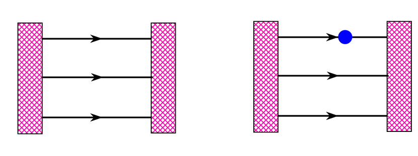
Figure 6: Graphs showing the normalization of a 3-quark component of a baryon (left) and the matrix element of a local operator denoted by a circle (right).

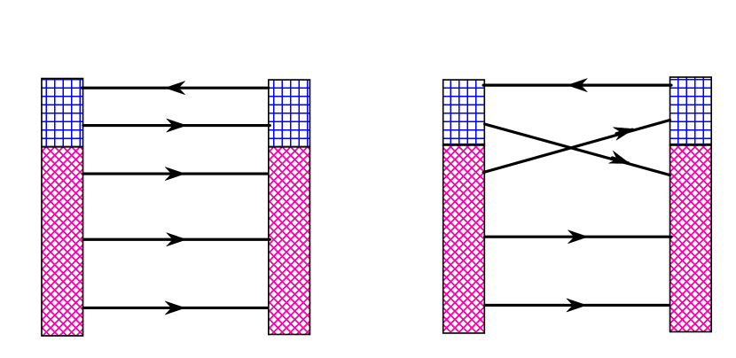
Figure 7: Direct (left) and exchange (right) contributions to the normalization of the 5-quark component of a baryon. The upper rectangles denote $Q\bar{Q}$ pairs.

In the matrix elements between the $3Q$ components the $b^{\dagger}b$ part of the current is passive as there are no antiquarks. The $a^{\dagger}a$ part is a sum over colors. As in the normalization, one gets the factor $6\cdot 6$ from all contractions. Let it be the third quark whose charge is measured: there is a factor of 3 from three quarks to which the charge operator can be applied, see Fig. 6. Denoting for short $\int\!(dp_{1-3})$ the integrals over momenta with the conservation $\delta$-functions as in eq. (49) we arrive at the following expression for the matrix element of the vector charge:

$$V^{(3)}(1\to 2) = \frac{(6\!\cdot\!6\!\cdot\!3)\!}{2}\,\delta^{k}_{l}\,T(1)^{f_{1}f_{2}f_{3}}_{j_{1}j_{2}j_{3},k}\,T(2)^{l_{1}l_{2}l_{3},l}_{f_{1}f_{2}g_{3}}\int\!(dp_{1-3})$$ (60)

$$\cdot\left[F^{j_{1}\sigma_{1}}(p_{1})F^{j_{2}\sigma_{2}}(p_{2})F^{j_{3}\sigma_{3}}(p_{3})\right]\,\left[F^{\dagger}_{l_{1}\sigma_{1}}(p_{1})F^{\dagger}_{l_{2}\sigma_{2}}(p_{2})F^{\dagger}_{l_{3}\tau_{3}}(p_{3})\right]\,\left[\delta^{\tau_{3}}_{\sigma_{3}}J^{g_{3}}_{f_{3}}\right].$$

One can easily check using eq. (14) that, say, for the $p\to n\rho^{+}$ transition, the above vector charge gives exactly the same expression as for the normalization (49). Therefore, the $g_{V}$ of this transition is unity, as it should be for the conserved vector current.

We consider here for simplicity only matrix elements of operators with zero momentum transfer. If it is non-zero, the generalization is obvious: one has to change the momentum of one of the quarks on which the operator acts, by the corresponding momentum transfer, and leave the rest quarks momenta unaltered.

For the axial transition, one replaces averaging over baryon spin by ${\textstyle{\frac{1}{2}}}(-\sigma_{3})^{k}_{l}$, and the axial charge operator is now $(-\sigma_{3})^{\tau_{3}}_{\sigma_{3}}$ instead of $\delta^{\tau_{3}}_{\sigma_{3}}$, see eq. (59). All the rest is the same as in eq. (60):

$$A^{(3)}(1\to 2) = \frac{(6\!\cdot\!6\!\cdot\!3)\!}{2}\,(-\sigma_{3})^{k}_{l}\,T(1)^{f_{1}f_{2}f_{3}}_{j_{1}j_{2}j_{3},k}\,T(2)^{l_{1}l_{2}l_{3},l}_{f_{1}f_{2}g_{3}}\int\!(dp_{1-3})$$ (61)

$$\!\cdot\!\left[F^{j_{1}\sigma_{1}}(p_{1})F^{j_{2}\sigma_{2}}(p_{2})F^{j_{3}\sigma_{3}}(p_{3})\right]\left[F^{\dagger}_{l_{1}\sigma_{1}}(p_{1})F^{\dagger}_{l_{2}\sigma_{2}}(p_{2})F^{\dagger}_{l_{3}\tau_{3}}(p_{3})\right]\!\left[(\!-\sigma_{3})^{\tau_{3}}_{\sigma_{3}}J^{g_{3}}_{f_{3}}\right]\!.$$

The result, however, is now different as the axial charge is not conserved. For example, for the $p\to n\pi^{+}$ transition one gets the expression identical to that for the normalization but with the factor 5/3. It means that we have obtained in the non-relativistic limit for the $3Q$ component of the nucleon $g_{A}^{(3)}(N)=5/3$. It is the well-known result of the non-relativistic quark model. However, it is modified by the relativistic corrections to the valence quark wave functions (35,36) and by the $5Q$ component of the nucleon.

X Five quarks: normalization, vector and axial charges

Already in the normalization of the $5Q$ Fock component of a baryon there are two types of contributions: direct and exchange ones, see Fig. 7. In the former, one contracts $a^{\dagger}$ from the pair wave function with an $a$ in the conjugate pair, and all the valence operators are contracted with each other. There are 6 such possibilities, and the contraction in color gives a factor $3\cdot 6$, all in all 108. In the exchange contributions, one contracts $a^{\dagger}$ from the pair with one of the three $a$’s from the valence level. Further on, $a$ from the conjugate pair is contracted with one of the three $a^{\dagger}$’s from the valence level. There are 18 such possibilities but the contraction in color gives now only a factor of 6. Therefore for the exchange contractions we also get a factor of 108 but with an overall negative sign as one has to anticommute fermion operators to get the exchange terms. As a result we obtain the following general expression for the normalization of the $5Q$ Fock component:

$${\cal N}^{(5)}(B) = \frac{108}{2}\,\delta^{k}_{l}\,T(B)^{f_{1}f_{2}f_{3}f_{4},j_{5}}_{j_{1}j_{2}j_{3}j_{4},f_{5},k}\,T(B)^{l_{1}l_{2}l_{3}l_{4},f_{5},l}_{f_{1}f_{2}g_{3}g_{4},l_{5}}\int\!(dp_{1-5})$$ (62)

$$\cdot F^{j_{1}\sigma_{1}}(p_{1})F^{j_{2}\sigma_{2}}(p_{2})F^{j_{3}\sigma_{3}}(p_{3})\,W^{j_{4}\sigma_{4}}_{j_{5}\sigma_{5}}(p_{4},p_{5})\,F^{\dagger}_{l_{1}\sigma_{1}}(p_{1})F^{\dagger}_{l_{2}\sigma_{2}}(p_{2})$$

$$\cdot \left[F^{\dagger}_{l_{3}\sigma_{3}}(p_{3})W^{l_{5}\sigma_{5}}_{\!c\,l_{4}\sigma_{4}}(p_{4},p_{5})\,\delta^{g_{3}}_{f_{3}}\delta^{g_{4}}_{f_{4}}-F^{\dagger}_{l_{3}\sigma_{4}}(p_{4})W^{l_{5}\sigma_{5}}_{\!c\,l_{4}\sigma_{3}}(p_{3},p_{5})\delta_{f_{4}}^{g_{3}}\delta_{f_{3}}^{g_{4}}\right]$$

where we have denoted

$$\int\!(dp_{1-5})=\int\!dz_{1-5}\,\delta(1-z_{1}-...-z_{5})\int\frac{d^{2}{\bf p_{1-5,\,\perp}}}{(2\pi)^{10}}\,(2\pi)^{2}\,\delta({\bf p_{1\perp}}+...+{\bf p_{5\perp}}).$$ (63)

The flavor tensor here is the group integral projecting the $5Q$ state onto a particular baryon, see eq. (44).

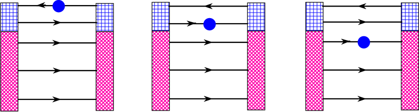
Figure 8: Direct contributions to the matrix element of an operator, in the 5-quark component of a baryon. The operator is applied to the antiquark (left), to the quark from the pair (middle) and to the quark from the valence level (right).

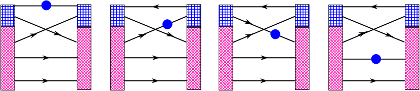
Figure 9: Four types of exchange contributions to the matrix element in the 5-quark component of a baryon.

The ratio of the normalization factors ${\cal N}^{(5)}/{\cal N}^{(3)}$ gives the probability to find a $5Q$ component in a mainly $3Q$ baryon. It depends on the mean field inside a baryon through the pair wave function $W$ (and is quadratic in the mean field), and on the particular baryon through its spin-flavor content $T$.

For the vector and axial transitions there are three basic contributions: one when the charge of the antiquark is measured, the second when the charge operator acts on the quark from the pair, and the third when it acts on one of the three valence quarks. These three types are further divided into the direct and exchange contributions (Figs. 8,9). We write below only the direct contributions; the exchange ones can be easily constructed from the graphs in Fig. 9.

The vector transition:

$$V^{(5){\rm direct}}(1\to 2) = \frac{108}{2}\,\delta^{k}_{l}\,T(1)^{f_{1}f_{2}f_{3}f_{4},j_{5}}_{j_{1}j_{2}j_{3}j_{4},f_{5},k}\,T(2)^{l_{1}l_{2}l_{3}l_{4},g_{5},l}_{f_{1}f_{2}g_{3}g_{4},l_{5}}\int\!(dp_{1-5})$$ (64)

$$\cdot F^{j_{1}\sigma_{1}}(p_{1})F^{j_{2}\sigma_{2}}(p_{2})F^{j_{3}\sigma_{3}}(p_{3})\,W^{j_{4}\sigma_{4}}_{j_{5}\sigma_{5}}(p_{4},p_{5})\,F^{\dagger}_{l_{1}\sigma_{1}}(p_{1})F^{\dagger}_{l_{2}\sigma_{2}}(p_{2})F^{\dagger}_{l_{3}\tau_{3}}(p_{3})\,W^{l_{5}\tau_{5}}_{\!c\,l_{4}\tau_{4}}(p_{4},p_{5})$$

$$\cdot \left[-\delta_{f_{3}}^{g_{3}}\delta_{f_{4}}^{g_{4}}J_{g_{5}}^{f_{5}}\delta^{\tau_{3}}_{\sigma_{3}}\delta^{\tau_{4}}_{\sigma_{4}}\delta^{\sigma_{5}}_{\tau_{5}}+\delta_{f_{3}}^{g_{3}}J_{f_{4}}^{g_{4}}\delta_{g_{5}}^{f_{5}}\delta^{\tau_{3}}_{\sigma_{3}}\delta^{\tau_{4}}_{\sigma_{4}}\delta^{\sigma_{5}}_{\tau_{5}}+3J_{f_{3}}^{g_{3}}\delta_{f_{4}}^{g_{4}}\delta_{g_{5}}^{f_{5}}\delta^{\tau_{3}}_{\sigma_{3}}\delta^{\tau_{4}}_{\sigma_{4}}\delta^{\sigma_{5}}_{\tau_{5}}\right].$$

The axial transition:

$$A^{(5){\rm direct}}(1\to 2) = \frac{108}{2}\,(-\sigma_{3})^{k}_{l}\,T(1)^{f_{1}f_{2}f_{3}f_{4},j_{5}}_{j_{1}j_{2}j_{3}j_{4},f_{5},k}\,T(2)^{l_{1}l_{2}l_{3}l_{4},g_{5},l}_{f_{1}f_{2}g_{3}g_{4},l_{5}}\int\!(dp_{1-5})$$ (65)

$$\cdot F^{j_{1}\sigma_{1}}(p_{1})F^{j_{2}\sigma_{2}}(p_{2})F^{j_{3}\sigma_{3}}(p_{3})\,W^{j_{4}\sigma_{4}}_{j_{5}\sigma_{5}}(p_{4},p_{5})\,F^{\dagger}_{l_{1}\sigma_{1}}(p_{1})F^{\dagger}_{l_{2}\sigma_{2}}(p_{2})F^{\dagger}_{l_{3}\tau_{3}}(p_{3})\,W^{l_{5}\tau_{5}}_{\!c\,l_{4}\tau_{4}}(p_{4},p_{5})$$

$$\cdot \left[\delta_{f_{3}}^{g_{3}}\delta_{f_{4}}^{g_{4}}J_{g_{5}}^{f_{5}}\delta^{\tau_{3}}_{\sigma_{3}}\delta^{\tau_{4}}_{\sigma_{4}}(\sigma_{3})^{\sigma_{5}}_{\tau_{5}}-\delta_{f_{3}}^{g_{3}}J_{f_{4}}^{g_{4}}\delta_{g_{5}}^{f_{5}}\delta^{\tau_{3}}_{\sigma_{3}}(\sigma_{3})^{\tau_{4}}_{\sigma_{4}}\delta^{\sigma_{5}}_{\tau_{5}}-3J_{f_{3}}^{g_{3}}\delta_{f_{4}}^{g_{4}}\delta_{g_{5}}^{f_{5}}(\sigma_{3})^{\tau_{3}}_{\sigma_{3}}\delta^{\tau_{4}}_{\sigma_{4}}\delta^{\sigma_{5}}_{\tau_{5}}\right],$$

where $J^{e}_{h}$ is the flavor content of the current defined in the previous section.

In the next sections we apply these general formulae to the calculation of the nucleon axial charge and the $\Theta^{+}$ width.

XI Five quarks: overlap integrals in the infinite momentum frame

It takes a few minutes by Mathematica to perform the contractions in eqs.(62,64,65) over all flavor ($f,g$), isospin ($j,l$) and spin ($\sigma,\tau$) indices. After all contractions are performed, one is left with scalar integrals over longitudinal ($z$) and transverse (${\bf p_{\perp}}$) momenta of the five quarks. The integrals over the relative transverse momenta in the $\bar{Q}Q$ pair are generally UV divergent, reflecting the divergence of the negative-energy Dirac sea of quarks (Fig. 1). In reality, this divergence is cut by the momentum-dependent dynamical quark mass $M(p)$, see eq. (2). Following Ref. SF where parton distributions in nucleons have been computed, satisfying all general sum rules, we shall mimic the fall-off of $M(p)$ by the Pauli–Villars cutoff at $M_{\rm PV}=557\,{\rm MeV}$ (this value is chosen from the requirement that the constant $F_{\pi}=93\,{\rm MeV}$ is reproduced from $M(0)=345\,{\rm MeV}$).

The pair wave function $W$ (28) is determined by the Fourier transforms of the mean chiral field $\Pi({\bf q})$ and $\Sigma({\bf q})$ (27): we find

$$\Pi({\bf q})^{i}_{j}=i\frac{(q^{a}\tau^{a})^{i}_{j}}{|{\bf q}|}\,\Pi(q),\qquad\Pi(q)=\frac{4\pi}{q^{2}}\int_{0}^{\infty}\!dr\,\sin P(r)(qr\cos qr-\sin qr)<0,$$ (66)

$$\Sigma({\bf q})^{i}_{j}=\delta^{i}_{j}\,\Sigma(q),\qquad\,\Sigma(q)=\frac{4\pi}{|q|}\int_{0}^{\infty}\!dr\,r\,\left(\cos P(r)-1\right)\,\sin qr<0.$$ (67)

Actually ${\bf q}$ is the 3-momentum of the $\bar{Q}Q$ pair, which in the infinite momentum frame is ${\bf q}=({\bf p_{4\perp}}+{\bf p_{5\perp}},\,(z_{4}+z_{5}){\cal M})$.

In the “direct” $5Q\to 5Q$ transitions (62,64,65) with zero momentum transfer the following four scalar integrals arise from squaring eq. (31), corresponding to i) the full square of $\Pi({\bf q})$, ii) the square of $\Sigma({\bf q})$, iii) the square of the third component $\Pi_{3}({\bf q})$, and iv) the mixed $\Pi_{3}({\bf q})\Sigma({\bf q})$ term:

$$K_{\pi\pi}\!\! = \frac{M^{2}}{2\pi}\!\!\int\!\!\frac{d^{3}{\bf q}}{(2\pi)^{3}}\,\Phi\left(\frac{q_{z}}{{\cal M}},{\bf q}_{\perp}\right)\,\theta(q_{z})q_{z}\,\Pi^{2}({\bf q})\!\int_{0}^{1}\!\!dy\!\int\!\frac{d^{2}{\bf Q}_{\perp}}{(2\pi)^{2}}\left[\frac{{\bf Q}_{\perp}^{2}+M^{2}}{\left({\bf Q}_{\perp}^{2}+M^{2}+y(1-y){\bf q}^{2}\right)^{2}}-(M\!\to\!M_{\rm PV})\right],$$ (68)

$$K_{\sigma\sigma}\!\! = \frac{M^{2}}{2\pi}\!\!\int\!\!\frac{d^{3}{\bf q}}{(2\pi)^{3}}\,\Phi\left(\frac{q_{z}}{{\cal M}},{\bf q}_{\perp}\right)\,\theta(q_{z})q_{z}\,\Sigma^{2}({\bf q})\!\int_{0}^{1}\!\!dy\!\int\!\frac{d^{2}{\bf Q}_{\perp}}{(2\pi)^{2}}\left[\frac{{\bf Q}_{\perp}^{2}+M^{2}(2y-1)^{2}}{\left({\bf Q}_{\perp}^{2}+M^{2}+y(1-y){\bf q}^{2}\right)^{2}}-(M\!\to\!M_{\rm PV})\right],$$ (69)

$$K_{33}\!\! = \frac{M^{2}}{2\pi}\!\!\int\!\!\frac{d^{3}{\bf q}}{(2\pi)^{3}}\,\Phi\left(\frac{q_{z}}{{\cal M}},{\bf q}_{\perp}\right)\,\theta(q_{z})\frac{q_{z}^{3}}{{\bf q}^{2}}\,\Pi^{2}({\bf q})\!\int_{0}^{1}\!\!dy\!\int\!\frac{d^{2}{\bf Q}_{\perp}}{(2\pi)^{2}}\left[\frac{{\bf Q}_{\perp}^{2}+M^{2}}{\left({\bf Q}_{\perp}^{2}+M^{2}+y(1-y){\bf q}^{2}\right)^{2}}-(M\!\to\!M_{\rm PV})\right],$$ (70)

$$K_{3\sigma}\!\! = \frac{M^{2}}{2\pi}\!\!\int\!\!\frac{d^{3}{\bf q}}{(2\pi)^{3}}\,\Phi\left(\frac{q_{z}}{{\cal M}},{\bf q}_{\perp}\right)\theta(q_{z})\frac{q_{z}^{2}}{|{\bf q}|}\,\Pi({\bf q})\Sigma({\bf q})\!\!\int_{0}^{1}\!\!\!dy\!\!\int\!\frac{d^{2}{\bf Q}_{\perp}}{(2\pi)^{2}}\!\left[\!\frac{{\bf Q}_{\perp}^{2}+M^{2}(2y-1)}{\left({\bf Q}_{\perp}^{2}+M^{2}+y(1-y){\bf q}^{2}\right)^{2}}-(M\!\to\!M_{\rm PV})\!\right]\!.$$ (71)

We have rearranged the integrals $dp_{1\!-\!5}$ such that we first integrate over the relative momenta inside the $\bar{Q}Q$ pair $y,{\bf Q}_{\perp}$ (see eq. (30)) and then over the 3-momentum ${\bf q}$ of the pair as a whole. As explained above, we regularize all integrals over the relative momenta by the Pauli–Villars subtraction. The step function $\theta(q_{z})$ ensures that in the IMF the longitudinal momentum carried by the pair is positive. By $\Phi(z,{\bf q}_{\perp})$ we denote the probability that three valence quarks “leave” the longitudinal fraction $z=z_{4}+z_{5}=q_{z}/{\cal M}$ and the transverse momentum ${\bf q}_{\perp}={\bf p}_{4\perp}+{\bf p}_{5\perp}$ to the $\bar{Q}Q$ pair:

$$\Phi(z,{\bf q}_{\perp}) = \int\frac{d^{2}{\bf p}_{1,2,3\,\perp}}{(2\pi)^{6}}dz_{1,2,3}\,(2\pi)^{2}\delta({\bf p}_{1\perp}+{\bf p}_{2\perp}+{\bf p}_{3\perp}+{\bf q}_{\perp})\,\delta(1-z-z_{1}-z_{2}-z_{3})\,h^{2}({\bf p}_{1})h^{2}({\bf p}_{2})h^{2}({\bf p}_{3}),$$

$${\bf p}_{1,2,3}=({\bf p}_{\perp\,1,2,3},p_{z\,1,2,3}),\qquad p_{z\,1,2,3}=z_{1,2,3}{\cal M}-E_{\rm lev}\,.$$

In the $3Q$ components of baryons, there are no additional $\bar{Q}Q$ pairs, and all quantities considered in Section IX are proportional to $\Phi(0,0)$. Since the normalization of the discrete-level wave function $h({\bf p})$ is arbitrary, we choose it such that $\Phi(0,0)=1$.

Let us give a few examples how the normalization, vector and axial charges of the $5Q$ components of baryons are expressed through the integrals (68-71) after all contractions in eqs.(62,64,65) are performed.

Nucleon normalization:

$${\cal N}^{(5)}(N)=\frac{18}{5}(11K_{\pi\pi}+23K_{\sigma\sigma}).$$ (73)

For the vector charge of the $n\to p$ transition one gets exactly the same expression, which demonstrates that the vector charge is conserved in each Fock component separately. The vector charge of the $\Theta^{+}\to K^{+}n$ transition turns out to be identically zero: it reflects the known fact that matrix elements of $SU(3)$ flavor generators between different irreducible representations, in this case between ${\bf\bar{1}0}$ and ${\bf 8}$, are zero; it serves as an additional check of eq. (64) since individual contributions in that equation are non-zero.

Nucleon axial charge:

$$A^{(5)}(p\to\pi^{+}n)=\frac{6}{25}(209K_{\pi\pi}+559K_{\sigma\sigma}-34K_{33}-356K_{3\sigma}).$$ (74)

$\Theta^{+}$ normalization:

$$N^{(5)}(\Theta)=\frac{36}{5}(K_{\pi\pi}+K_{\sigma\sigma}).$$ (75)

Axial charge of the $\Theta^{+}\to K^{+}n$ transition:

$$A^{(5)}(\Theta^{+}\to K^{+}n)=\frac{6}{5}\sqrt{\frac{3}{5}}(-7K_{\pi\pi}-5K_{\sigma\sigma}+8K_{33}+28K_{3\sigma}).$$ (76)

Notice that the coefficients are an order of magnitude less in the $\Theta^{+}$ than in the nucleon case. It should be noted that we have independently derived eqs. (73-76) in another way by applying the charge operators directly to the five quarks and using the $SU(3)$ Clebsch–Gordan machinery for projecting the $5Q$ states onto the baryons in question. Since this technique is different from the one presented here, it serves as a powerful check of the above expressions. We now proceed to evaluate them numerically.

XII Numerical results

For the numerical evaluation of the integrals involved in the $5Q$ matrix elements we use the quark mass $M=345\,{\rm MeV}$, the self-consistent profile function (5), the Pauli–Villars mass $M_{\rm PV}=557\,{\rm MeV}$, and the baryon mass ${\cal M}=1207\,{\rm MeV}$, as it follows for the “classical” mass (i.e. without quantum corrections) in the mean field approximation DPPrasz . The self-consistent pseudoscalar $\Pi({\bf q})$ and scalar $\Sigma({\bf q})$ fields, as given by eqs.(66,67) are plotted in Fig. 10. The probability distribution $\Phi(z,{\bf q}_{\perp})$ (XI) that the $\bar{Q}Q$ pair carries the fraction $z$ of the baryon momentum and the transverse momentum ${\bf q}_{\perp}$ is plotted in Fig. 11.

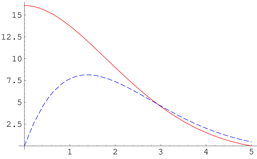
Figure 10: The self-consistent pseudoscalar $-|{\bf q}|\Pi({\bf q})$ (solid) and scalar $-|{\bf q}|\Sigma({\bf q})$ (dashed) fields in baryons in the momentum representation. The horizontal axis is in units of $M=345\,{\rm MeV}$.

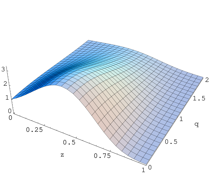
Figure 11: The probability distribution $\Phi(z,{\bf q}_{\perp})$ that the $\bar{Q}Q$ pair carries the fraction $z$ of the baryon momentum and the transverse momentum ${\bf q}_{\perp}$ plotted in units of $M=345\,{\rm MeV}$.

With these functions, the numerical evaluation of the integrals (68-71) yields

$$K_{\pi\pi}=0.0623,\qquad K_{\sigma\sigma}=0.0284,\qquad K_{33}=0.0372,\qquad K_{3\sigma}=0.0333.$$ (77)

Putting these values into eqs.(73-76) we obtain

Nucleon $5Q$ normalization:

$${\cal N}^{(5)}(N)=4.813.$$ (78)

Nucleon $5Q$ axial charge:

$$A^{(5)}(p\to\pi^{+}n)=3.779.$$ (79)

$\Theta^{+}$ $5Q$ normalization:

$$N^{(5)}(\Theta)=0.652.$$ (80)

$\Theta^{+}$ $5Q$ axial charge:

$$A^{(5)}(\Theta^{+}\to K^{+}n)=0.607.$$ (81)

One has to add the $3Q$ nucleon normalization computed from eq. (49)

$${\cal N}^{(3)}(N)=9\Phi(0,0)=9$$ (82)

and the $3Q$ nucleon axial charge computed from eq. (61)

$$A^{(3)}(p\to\pi^{+}n)=15\Phi(0,0)=15,$$ (83)

from where it follows that in the non-relativistic $3Q$ approximation the nucleon axial charge is

$$g_{A}^{(3)}(N)=\frac{A^{(3)}(p\to\pi^{+}n)}{{\cal N}^{(3)}(N)}=\frac{5}{3}\approx 1.67$$ (84)

which is the well-known result of the non-relativistic quark model.

In the $5Q$ approximation, the nucleon axial charge is

$$g_{A}^{(5)}(N)=\frac{A^{(3)}(p\to\pi^{+}n)+A^{(5)}(p\to\pi^{+}n)}{{\cal N}^{(3)}(N)+{\cal N}^{(5)}(N)}\approx 1.36$$ (85)

which brings it closer to the experimental value $g_{A}(N)=1.27$. The account for any number of pairs and for relativistic corrections in the $1/N_{c}$ expansion brings $g_{A}$ very close to the experimental value corrNc1 .

We note that the ratio of the $5Q$ to the $3Q$ normalization in the nucleon is

$$\frac{{\cal N}^{(5)}(N)}{{\cal N}^{(3)}(N)}=0.535\approx 50\%.$$ (86)

On the one hand, it means that the $5Q$ Fock component of the nucleon is quite substantial but on the other hand it implies that antiquarks carry roughly only

$$\frac{0\cdot 1+\frac{1}{5}\cdot{\textstyle{\frac{1}{2}}}}{1+{\textstyle{\frac{1}{2}}}}\approx 7\%$$

of the nucleon momentum, assuming the antiquark carries $1/5$ of the momentum in the $5Q$ component footnote2 . We have not evaluated the $7Q...$ normalization in the nucleon (which would follow from expanding the coherent exponent in eq. (12) to higher orders) but expect that higher Fock components are suppressed, roughly, by factorials following from the expansion of the exponent. At large $N_{c}$, however, there would be on the average ${\cal O}(N_{c})$ $\bar{Q}Q$ pairs in the nucleon.

Turning to the axial constant of the $\Theta^{+}\to KN$ transition we obtain

$$g_{A}(\Theta\to KN)=\frac{A^{(5)}(\Theta^{+}\to K^{+}n)}{\sqrt{N^{(5)}(\Theta)}\,\sqrt{{\cal N}^{(3)}(N)+{\cal N}^{(5)}(N)}}=0.202$$ (87)

being substantially less than the nucleon axial charge computed in the same approximation. The quantity is similar in spirit (and magnitude) not to the nucleon axial coupling itself but to its change as due to the $5Q$ component in the nucleon, $g_{A}^{(3)}(N)-g_{A}^{(5)}(N)=0.31$. It is additionally suppressed by the $SU(3)$ group factors for the ${\bf\overline{10}}\to{\bf 8}$ transition.

Assuming the approximate $SU(3)$ chiral symmetry (which was the base for using the $\Theta^{+}$ wave function (46) in the first place) one can get the $\Theta^{+}\to KN$ pseudoscalar coupling from the generalized Goldberger–Treiman relation

$$g_{\Theta KN}=\frac{g_{A}(\Theta\to KN)(M_{\Theta}+M_{N})}{2F_{K}}=2.24$$ (88)

where we use $M_{\Theta}=1530\,{\rm MeV},\,M_{N}=940\,{\rm MeV},\,F_{K}=1.2F_{\pi}=112\,{\rm MeV}$. Knowing the transition pseudoscalar constant one can evaluate the $\Theta^{+}$ width from the general expression for the ${\textstyle{\frac{1}{2}}}^{+}$ hyperon decay Okun

$$\Gamma_{\Theta}=2\cdot\frac{g_{\Theta KN}^{2}|{\bf p}|}{8\pi}\,\frac{(M_{\Theta}-M_{N})^{2}-m_{K}^{2}}{M_{\Theta}^{2}}=4.44\,{\rm MeV}$$ (89)

where $|{\bf p}|=\sqrt{(M_{\Theta}^{2}-M_{N}^{2}-m_{K}^{2})^{2}-4M_{N}^{2}m_{K}^{2}}/2M_{\Theta}=254\,{\rm MeV}$ is the kaon momentum in the decay ($m_{K}=495\,{\rm MeV}$), and we have put the factor 2 to account for the equal-probability $K^{+}n$ and $K^{0}p$ decays.

XIII Theoretical uncertainties

Unfortunately, in baryon physics we deal with a truly strong interaction case, meaning that all dimensionless quantities are generally speaking of the order of unity. There is no really small algebraic parameter in sight that would allow some kind of perturbative expansion. We have argued in the Introduction that $1/N_{c}$ can be considered as a formal small parameter justifying the use of the Relativistic Mean Field Approximation. However, it is definitely not small enough when it comes to “kinematical” factors related to the rotational states of the mean-field baryons. Therefore, we treat the octet, decuplet and antidecuplet baryons as it should be at $N_{c}=3$, rather than dealing with the large-$N_{c}$ prototypes of those multiplets. We expect that the accuracy of this mixed logic is at the level of $1/(2\pi N_{c})\sim 10\%$.

Another source of the uncertainty is the present lack of knowledge of the exact low-energy effective action (2), in particular of the exact dynamical quark mass $M(p)$. We have mimicked the fall-off of this function at large momenta by introducing the Pauli–Villars cutoff such that the $F_{\pi}$ constant and the chiral condensate $<\!\bar{q}q\!>$ are reproduced. From the experience in calculating various observables in the Chiral Quark Soliton Model DP-CQSM we estimate the ensuing error as $\sim 15\%$. Thus, the resulting accuracy of the Relativistic Mean Field Approximation with exact account for the rotational wave functions of baryons, is expected to be about $20\%$, and this is indeed the typical accuracy with which formfactors, magnetic moments, parton distributions etc. have been computed in the model; in many cases the accuracy is actually much better but we quote here the pessimistically expected accuracy.

When dealing with hyperons containing strange quarks, one has to decide how does one treat the mass $m_{s}$. Theoretically speaking, there are two small parameters, $1/N_{c}$ and $m_{s}/\Lambda$ where $\Lambda$ is the characteristic scale of the strong interactions. Before choosing a calculational scheme one has to decide which of the two parameters is “smaller”. One observes that the mass splittings in the baryon octet and decuplet are ${\cal O}(m_{s}N_{c})$ and are somewhat less than the splitting between octet and decuplet centers, which is ${\cal O}(\Lambda/N_{c})$. Also, the Gell-Mann–Okubo relations are satisfied to the 0.5% accuracy, which can be algebraically written as ${\cal O}(m_{s}^{2}/\Lambda^{2})$. It indicates that the former parameter is larger than the latter, moreover it is not unreasonable to say that the strange quark mass is very small, $m_{s}={\cal O}(\Lambda/N_{c}^{2})$. In practical terms it means that in baryons, $m_{s}$ can be treated as a perturbation in most cases. In this paper, we have actually used the chiral limit, $m_{s}=0$, i.e. the zeroth order of that perturbation series. Computing first-order corrections in $m_{s}$ to the observables does not cause serious difficulties, see e.g. Refs. hyperons ; DPP97 , but we have not done it here. The penalty is expected at the $20\%$ level.

Within the Relativistic Mean Field Approximation, there arises a new important dimensionless parameter, namely $\epsilon=E_{\rm lev}/M$ where $M=M(0)$ is the dynamical quark mass at zero virtuality and $E_{\rm lev}$ is the quark bound-state level generated by the self-consistent chiral field, see eq. (6). If $\epsilon\approx 1$, the valence quarks in baryons are non-relativistic, the upper $s$-wave Dirac component of their wave function $h(r)$ is much larger than the lower $p$-wave component $j(r)$, and the number of additional $\bar{Q}Q$ pairs in baryons tends to zero. In this limit the $\Theta^{+}$ width goes to zero DPP97 , which can be also seen from the equations of the previous section, in particular from eq. (87): the numerator in that equation ($A^{(5)}$) is proportional to the number of the $\bar{Q}Q$ pairs while the denominator ($\sqrt{N^{(5)}(\Theta)}$) is proportional to its square root. Consequently, the width $\Gamma_{\Theta}$ is proportional to the number of $\bar{Q}Q$ pairs in ordinary baryons and vanishes in the non-relativistic limit $\epsilon\to 1$.

Actually in our estimates in Section XII, we have systematically used the first-order perturbation theory in the “relativism” of valence quarks or, mathematically speaking, in $1-\epsilon$. Namely, we have

• ignored the lower component of the valence wave function $j(r)$

• ignored the distortion of the valence wave function by the sea, eq. (36)

• used the approximate expression for the pair wave function (28)

• computed the direct but neglected the exchange diagrams when evaluating the $5Q$ normalization and transition matrix elements, shown in Fig. 7 and 9

• neglected the $7Q,9Q...$ components in baryons.

It is difficult to evaluate the errors of these approximations before the neglected corrections are computed (which is surely feasible as all corrections are well defined above, but it has not been done). Unfortunately, the uncertainty associated with this non-relativistic approximation is expected to be large since the actual expansion parameter $1-\epsilon=0.42$ is poor. Another sign that the nucleon is in fact a relativistic system comes from the $50\%$ ratio of the $5Q$ to the $3Q$ normalization. Treating the relativistic system in the first order in the “relativism”, is undoubtedly the main source of the uncertainty in our numerical estimates.

Assuming that the uncertainties mentioned above are “statistically independent”, we estimate the error in computing the transition coupling $g_{\Theta KN}$ as

$$\sqrt{0.2^{2}+0.2^{2}+0.42^{2}}=0.5$$

implying a 100% error in the width.

To get a feeling of the accuracy of our estimates, we have redone the calculations of Section XII replacing the probability distribution $\Phi(z,{\bf q}_{\perp})$ introduced in Section XI by a flat one. This is a legitimate assumption within the Mean Field Approximation as it corresponds to ignoring the restriction following from the quark momentum conservation. We remind the reader that we have used the value of the baryon mass ${\cal M}=1207\,{\rm MeV}$ instead of, say, $940\,{\rm MeV}$: the difference is believed to be partially due to adding the momentum conservation correction to the Mean Field result Goeke-momentum . Therefore, it may seem to be more logical to ignore the quark momentum conservation systematically throughout the calculations.

With this assumption, the evaluation of the $5Q$ matrix elements (68-71) is very easy and we obtain, instead of eq. (77),

$$K_{\pi\pi}=0.0428,\qquad K_{\sigma\sigma}=0.0235,\qquad K_{33}=0.0214,\qquad K_{3\sigma}=0.0226.$$ (90)

These numbers lead, via eqs. (73-76), to the following values of the physical quantities:

$$\frac{{\cal N}^{(5)}(N)}{{\cal N}^{(3)}(N)}=0.405,\qquad g_{A}^{(5)}(N)=1.44,$$ (91)

which are not qualitatively different from the estimates (85,86). However, the $\Theta^{+}$ width appears to be quite sensitive to the change:

$$g_{A}(\Theta\to KN)=0.146,\qquad\Gamma_{\Theta}=2.32\,{\rm MeV},$$ (92)

the width turning out nearly twice smaller than that of Section XII. It gives the idea of the accuracy of our estimate.

Probably the worse error in our estimate of the $\Theta^{+}$ width arises from neglecting the exchange diagrams in matrix elements, see Figs. 7 and 9. As a rule, their account in processes involving fermions reduces matrix elements. It should be also noticed that the mass difference between the $\Theta^{+}$ and the nucleon is not small whereas we have estimated the transition amplitude at zero momentum transfer. One would hence expect that there is an additional formfactor-like reduction of the $\Theta^{+}\to KN$ transition amplitude.

Therefore, one can well imagine that the $\Theta^{+}$ width (92) is further reduced, maybe even below the $1\,{\rm MeV}$ value. We do not think that taking into account the $7Q...$ components in the transition matrix elements will seriously alter the $5Q$ estimates.

Pinning down the $\Theta^{+}$ width even inside a wide 50% error margin requires much more work than presented here. Nevertheless, the estimate that $\Gamma_{\Theta}$ is in a few MeV range seems to be safe. It follows from the relative suppression of $\bar{Q}Q$ pairs in the nucleon, and from the $SU(3)$ group suppression in the $\Theta^{+}\to KN$ transition.

XIV Conclusions

Ordinary baryons are not made of three quarks only but have a substantial component with additional $\bar{Q}Q$ pairs. For some observables, additional $\bar{Q}Q$ pairs change the naive $3Q$ results by only 20% (like in the case of the nucleon axial constant) but for some other observables they change the naive result by a factor of $3\!-\!4$ (as in the case of the spin carried by quarks or the nucleon $\sigma$ term). Hence it is imperative to learn how to work with higher Fock components in baryons.

It is imperative not only for practical but for simple theoretical reasons. Assuming there are just three quarks in a baryon and wishing to write down their wave function, one realizes that one cannot “measure” (and hence mathematically describe) the quark position to an accuracy better than the Compton wave length of a pion ($1.4\,{\rm fm}$), since by uncertainty principle one then produces a pion or an additional $\bar{Q}Q$ pair. Since the baryon size is $1\,{\rm fm}$, there is literally no room for the just-three-quarks description of a baryon. The uncertainty principle demands that baryons should be described as containing an indefinite number of $\bar{Q}Q$ pairs. The only question is quantitative: how many are there $\bar{Q}Q$ pairs, and what are their wave functions footnote3 .

Moving to this uncharted territory, one has to satisfy certain general conditions as the relativistic invariance (since pair production is a relativistic effect) and the completeness of states, needed to guarantee that parton distributions, including antiquarks, are positive-definite and are subject to sum rules following from the conservation laws for the baryon charge, axial current, etc. Relativistic invariance and the completeness of states can be achieved only in a relativistic quantum field theory. A field-theoretic model of baryons, which takes into account the infinite number of degrees of freedom and in which these general conditions are automatically met, is the Chiral Quark Soliton Model DP-CQSM , an alias for the Relativistic Mean Field Approximation.

Using this model, we have presented a technique allowing to write down explicitly the $3Q$, $5Q$, $7Q...$ wave functions of the octet, decuplet and antidecuplet baryons. In the exotic antidecuplet the $3Q$ component is, of course, absent, but its leading $5Q$ component is space-wise similar to the non-leading $5Q$ component of the nucleon. The technique is mathematically equivalent to the “valence quarks plus Dirac continuum” method exploited previously, but brings the mean field approach even closer to the language of the quark wave functions used by many people. We have shown that the standard $SU(6)$ wave functions are easily reproduced for the $3Q$ components of the octet and decuplet baryons, if one assumes the non-relativistic limit. However, we have given explicit formulae for the relativistic corrections to the $3Q$ wave function, and also for the $5Q$ wave function of the nucleon and of the exotic $\Theta^{+}$. Having patience one can go further and write down e.g. the 19-quark component of the proton or the 7-quark component of the exotic $\Xi^{--}$.

It is important that the $\bar{Q}Q$ pair in the $5Q$ Fock component of any baryon, be it the nucleon or the $\Theta^{+}$, is added in the form of a chiral field, which costs little energy. This is the reason why the $5Q$ component in the nucleon turns out to be substantial, and why the exotic $\Theta^{+}$ baryon whose Fock decomposition starts from the $5Q$ component, is expected to be light. The energy penalty for making a pentaquark would be exactly zero in the chiral limit and were baryons infinitely large. In reality, to make e.g. the $\Theta^{+}$ from the nucleon, one has to create a quasi-Goldstone K-meson and to confine it inside the baryon of the size $\geq 1/M$. It costs roughly

$$m(\Theta)-m(N)\approx\sqrt{m_{K}^{2}+{\bf p}^{2}}\leq\sqrt{495^{2}+345^{2}}=603\,{\rm MeV}.$$ (93)

Therefore, one should expect the exotic $\Theta^{+}$ around 1540 MeV. The existence of the lightest degree of freedom in QCD, namely the pseudo-Goldstone fields, is ignored in the non-relativistic constituent quark models, which leads to the overestimate of the $\Theta^{+}$ mass by typically $500\,{\rm MeV}$ D04-Osaka .

Having presented the general formalism for computing observables for the $3Q$ as well as for higher Fock components, we have applied it to several cases of immediate interest. We have estimated the normalization of the $5Q$ component of the nucleon as about 50% of the $3Q$ component, meaning that about $1/3$ of the time the nucleon is “made of” five quarks. We have also shown that the account for the $5Q$ component in the nucleon moves its axial charge from the naive non-relativistic value of $5/3$ much closer to the experimental value.

Another case of interest is the width of the exotic $\Theta^{+}$ baryon: if it exists, why is it so narrow? The best direct experimental limit is $\Gamma_{\Theta}<9\,{\rm MeV}$ Dolgolenko , however indirect estimates narrow indicate that the width can be as small as $1\,{\rm Mev}$ or even less. Such a narrow width for a strongly decaying baryon some $100\,{\rm MeV}$ above the threshold, is the main surprise about the $\Theta^{+}$. Since the original narrow-width estimate $\Gamma_{\Theta}<15\,{\rm MeV}$ DPP97 (or, to be more precise, $3.6<\Gamma_{\Theta}<11.4\,{\rm MeV}$ DPP04 ) based on the Chiral Quark Soliton Model, we have made here the first estimate of the axial constant for the $\Theta^{+}\to KN$ transition, based on the direct computation of the $5Q$ matrix element within the same logic. We have shown that the $\Theta^{+}$ width is proportional to the number of $\bar{Q}Q$ pairs in nucleons and is thus naturally suppressed, as compared to the expected widths of baryons with the dominant $3Q$ component. Assuming the $SU(3)$ symmetry, the $\Theta^{+}$ width is additionally suppressed by the $SU(3)$ Clebsch–Gordan factors.

In this first direct estimate using the $5Q$ wave functions of the $\Theta^{+}$ and of the nucleon, we have made several approximations summarized in Section XIII. The worse approximations can be eliminated by further work outlined in the paper but at the moment they lead to a large theoretical uncertainty in the $\Theta^{+}$ width. Depending on the way we impose the approximation, we obtain $\Gamma_{\Theta}\approx 2-4\,{\rm MeV}$, with a high probability that it is further reduced by taking into account the quark exchange processes in the $\Theta^{+}\to KN$ transition, and the formfactor-like suppression in this finite momentum transfer decay (both of which we neglected). Therefore, the $\Theta^{+}$ width of a few MeV appears naturally within the Relativistic Mean Field Approximation, without any parameter fixing.

We believe that the presented formalism has a broad field of applications, apart from exotic baryons. One kind of applications has been already started in Ref. PP-IMF and involves exclusive processes, nucleon distribution amplitudes, parton distributions for a fixed number of quarks, and the like. Another kind of applications is for low energies. One can compute any type of transition amplitudes between various Fock components of baryons, including the relativistic effects, the effects of the $SU(3)$ symmetry violation, mixing of multiplets, and so on.

Acknowledgements

V.P. is grateful to NORDITA for kind hospitality during his visit in September–October 2003 when this work has been started. The work of V.P. has been supported in part by the Russian Government grant 1124.2003.2.

Appendix A Parametrization of $SU(N)$ matrices

In this Appendix we construct by induction a parametrization of a general unitary unimodular $SU(N)$ matrix in terms of $N^{2}-1$ “Euler angles”, and write down the invariant Haar measure over the group in terms of these angles. The construction has been prompted by the parametrization of the $SU(3)$ group by Mathur and Sen MS .

The idea is to write iteratively a general $SU(N)$ matrix as

$$R_{N}=S_{N}R_{N-1}$$ (94)

where $R_{N-1}$ is a general $SU(N-1)$ matrix with $(N-1)^{2}-1$ parameters and $S_{N}$ is an $SU(N)$ matrix of a special kind with only $2N-1$ parameters belonging to the sphere $S^{2N-1}$. It gives the full parametrization of a general $SU(N)$ matrix with $N^{2}-1$ parameters. Accordingly, the invariant integration measure over the $SU(N)$ group is presented as a product of measures over the spheres $S^{3}\times S^{5}\times...\times S^{2N-1}$.

One starts from the $SU(2)$ group whose parametrization as a $3d$ sphere $S^{3}$ is well known: one writes a general $SU(2)$ matrix as

$$S_{2}=\left(\begin{array}[]{cc}e^{-i\alpha_{11}}\cos\phi_{1}&e^{i\alpha_{12}}\sin\phi_{1}\\ -e^{-i\alpha_{12}}\sin\phi_{1}&e^{i\alpha_{11}}\cos\phi_{1}\end{array}\right)$$ (95)

where the last column in $S_{2}$ can be viewed as a $2d$ complex vector $v_{2}=(z^{1},z^{2})$ normalized as $|z^{1}|^{2}+|z^{2}|^{2}=1$, which defines an $S^{3}$ sphere. The first column is the orthogonal vector $v_{1}^{i}=\epsilon^{ij}\bar{v}_{2j}$. The group measure can be written as an integral over the $S^{3}$ sphere,

$$\frac{1}{\pi^{2}}\int dz^{1}d\bar{z}^{1}dz^{2}d\bar{z}^{2}\,\delta(|z^{1}|^{2}+|z^{2}|^{2}-1),$$ (96)

or, explicitly in terms of three angles, as

$$\frac{1}{2\pi^{2}}\int_{0}^{\frac{\pi}{2}}d\phi_{1}\,\sin\phi_{1}\cos\phi_{1}\int_{0}^{2\pi}d\alpha_{11}\int_{0}^{2\pi}d\alpha_{12}\qquad(=1).$$ (97)

To construct a general $SU(3)$ matrix using the recipe (94) we first make a $3\times 3$ matrix $R_{2}$ putting $S_{2}$, say, in its left upper corner,

$$R_{2}=\left(\begin{array}[]{cc}S_{2}&\begin{array}[]{c}0\\ 0\end{array}\\ \begin{array}[]{cc}0&0\end{array}&1\end{array}\right)\,,$$ (98)

and define

$$R_{3}=S_{3}R_{2},\qquad S_{3}=\left(\begin{array}[]{ccc}e^{i\alpha_{23}}\cos\theta&0&e^{i\alpha_{23}}\sin\theta\\ -e^{i\alpha_{22}}\sin\theta\sin\phi_{2}&e^{-i\alpha_{21}-i\alpha_{23}}\cos\phi_{2}&e^{i\alpha_{22}}\cos\theta\sin\phi_{2}\\ -e^{i\alpha_{21}}\sin\theta\cos\phi_{2}&-e^{-i\alpha_{22}-i\alpha_{23}}\sin\phi_{2}&e^{i\alpha_{21}}\cos\theta\cos\phi_{2}\end{array}\right).$$ (99)

The last column in $S_{3}$ can be viewed as a $3d$ complex vector $v_{3}=(z^{1},z^{2},z^{3})$ normalized to $|z^{1}|^{2}+|z^{2}|^{2}+|z^{3}|^{2}=1$, which defines an $S^{5}$ sphere. The three columns are constructed as (complexified) orts in spherical coordinates: $v_{1}\sim e_{r},\,v_{2}\sim e_{\phi},v_{3}\sim e_{\theta}$. There is of course a freedom of choosing the orts and the angles; we use part of this freedom in such a way that $R_{3}={\bf 1_{3}}$ when all angles are set to zero.

The measure on $S^{5}$ can be written as

$$\frac{2}{\pi^{3}}\int dz^{1}d\bar{z}^{1}dz^{2}d\bar{z}^{2}dz^{3}d\bar{z}^{3}\,\delta(|z^{1}|^{2}+|z^{2}|^{2}+|z^{3}|^{2}-1),$$ (100)

or, explicitly in terms of five angles, as

$$\frac{1}{\pi^{3}}\int_{0}^{\frac{\pi}{2}}d\theta\,\cos^{3}\theta\sin\theta\int_{0}^{\frac{\pi}{2}}d\phi_{2}\,\sin\phi_{2}\cos\phi_{2}\int_{0}^{2\pi}d\alpha_{21}\int_{0}^{2\pi}d\alpha_{22}\int_{0}^{2\pi}d\alpha_{23}\qquad(=1).$$ (101)

The integrations limits are chosen such that the $S^{5}$ sphere is covered once.

The full $SU(3)$ measure is found in the standard way: one constructs the metric tensor

$$g_{mn}=\mbox{Tr}\,\frac{\partial R_{3}}{\partial_{\beta^{m}}}\frac{\partial R_{3}^{\dagger}}{\partial_{\beta^{n}}},\qquad\beta^{m}=\alpha_{11},\alpha_{12},\phi_{1},\alpha_{21},\alpha_{22},\alpha_{23},\phi_{2},\theta,\quad m,n=1...8;$$ (102)

then the $SU(3)$ measure is

$$\sqrt{\det g}\sim(\sin\phi_{1}\cos\phi_{1})\cdot(\cos^{3}\theta\sin\theta\sin\phi_{2}\cos\phi_{2})$$ (103)

i.e. it is factorized into the product of the measures over the spheres $S^{3}$ and $S^{5}$, see eqs.(97,101). All group integrals in Appendix B can be performed directly using the above parametrization of the $SU(2)$ and $SU(3)$ matrices and the above Haar measure. In fact we have checked the results of Appendix B in this way.

The construction can be iteratively generalized to higher $SU(N)$ groups in such a way that the group parameter space is a direct product of the spheres $S^{3}\times S^{5}\times\ldots S^{2N-1}$ with the total number of parameters $\sum_{J=1}^{N-1}(2J+1)=N^{2}-1$, as it should be for the $SU(N)$ group. For example, a parametrization of $R\in SU(4)$ is

$$R_{4} = S_{4}R_{3},$$ (104)

$$S_{4}\!\! \!\!=\!\! \!\!\left(\begin{array}[]{cccc}\cos\chi e^{i\alpha_{34}}&0&0&-\sin\chi e^{i\alpha_{34}}\\ \sin\chi\sin\theta_{3}e^{i\alpha_{33}}&\cos\theta_{3}e^{i\alpha_{33}}&0&\cos\chi\sin\theta_{3}e^{i\alpha_{33}}\\ \sin\chi\cos\theta_{3}\sin\phi_{3}e^{i\alpha_{32}}&-\sin\theta_{3}\sin\phi_{3}e^{i\alpha_{32}}&\cos\phi_{3}e^{-i\alpha_{31}-i\alpha_{33}-i\alpha_{34}}&\cos\chi\cos\theta_{3}\sin\phi_{3}e^{-i\alpha_{32}}\\ \sin\chi\cos\theta_{3}\cos\phi_{3}e^{i\alpha_{31}}&-\sin\theta_{3}\cos\phi_{3}e^{i\alpha_{31}}&-\sin\phi_{3}e^{-i\alpha_{32}-i\alpha_{33}-i\alpha_{34}}&\cos\chi\cos\theta_{3}\cos\phi_{3}e^{i\alpha_{31}}\end{array}\right)\,,$$ (109)

and $R_{3}$ is the block-diagonal $4\times 4$ matrix with the general $SU(3)$ matrix (99) in the left upper corner and unity in the right lower corner. We thus add 7 new parameters to the previous 8 of the $SU(3)$ parametrization. The columns of $S_{4}$ are complex orts in spherical coordinates, $e_{r},e_{\theta},e_{\phi},e_{\chi}$. Denoting the last column $v_{4}=(z^{1},z^{2},z^{3},z^{4})$ the integration measure is that of a sphere $S^{7}$:

$$\int\!dz^{1}d\bar{z}^{1}\ldots dz^{4}d\bar{z}^{4}\,\delta(|z^{1}|^{2}+\ldots|z^{4}|^{2}-1)\sim\int\!\cos^{5}\chi\sin\chi\,\cos^{3}\theta_{3}\sin\theta_{3}\cos\phi_{3}\sin\phi_{3}\,d\chi d\theta_{3}d\phi_{3}d\alpha_{31}d\alpha_{32}d\alpha_{33}d\alpha_{34}.$$ (110)

The full $SU(4)$ measure built from the general rule (102) (where now there are 15 angles) is factorized into the product of measures over the $S^{3},S^{5}$ and $S^{7}$ spheres.

Appendix B Group integrals

In this Appendix, we give a list of group integrals used in the main text, over the Haar measure of the $SU(N)$ group, normalized to unity, $\int dR=1$.

For any $SU(N)$ one has

$$\int dR\,R^{f}_{i}=0,\qquad\int dR\,R^{\dagger\,i}_{f}=0,\qquad\int dR\,R^{f}_{i}\,R^{\dagger\,j}_{g}=\frac{1}{N}\delta^{f}_{g}\,\delta^{j}_{i}.$$ (111)

For $N=2$ the following group integral is non-zero:

$$\int dR\,R^{f}_{i}\,R^{g}_{j}=\frac{1}{2}\epsilon^{fg}\,\epsilon_{ij}.$$ (112)

For $N>2$ this integral is zero; its analog in $SU(3)$ is

$$\int dR\,R^{f}_{i}\,R^{g}_{j}\,R^{h}_{k}=\frac{1}{6}\epsilon^{fgh}\,\epsilon_{ijk}.$$ (113)

On the contrary, in $SU(2)$ it is zero.

The general method of finding integrals of several matrices $R,R^{\dagger}$ is as follows. The result of an integration over the invariant measure can be only invariant tensors which, for the $SU(N)$ group, can be built solely from the Kronecker $\delta$ and Levi–Civita $\epsilon$ tensors. One constructs the supposed tensor of a given rank as a combination of $\delta$’s and $\epsilon$’s, satisfying the symmetry relations following from the integral in question. The indefinite coefficients in the combination are then found from contracting both sides with various $\delta$’s and $\epsilon$’s and thus by reducing the integral to a previously derived one.

For any $SU(N)$ group one has

$$\int dR\,R^{f_{1}}_{i_{1}}\,R^{\dagger\,j_{1}}_{g_{1}}\,R^{f_{2}}_{i_{2}}\,R^{\dagger\,j_{2}}_{g_{2}}=\frac{1}{N^{2}-1}\left[\delta^{f_{1}}_{g_{1}}\delta^{f_{2}}_{g_{2}}\left(\delta^{i_{1}}_{j_{1}}\delta^{i_{2}}_{j_{2}}-\frac{1}{N}\delta^{i_{1}}_{j_{2}}\delta^{i_{2}}_{j_{1}}\right)+\delta^{f_{1}}_{g_{2}}\delta^{f_{2}}_{g_{1}}\left(\delta^{i_{1}}_{j_{2}}\delta^{i_{2}}_{j_{1}}-\frac{1}{N}\delta^{i_{1}}_{j_{2}}\delta^{i_{2}}_{j_{1}}\right)\right]$$ (114)

since its contraction with, say, $\delta^{g_{1}}_{f_{1}}$ must reduce it to eq. (111).

In $SU(2)$ there is an identity

$$\delta^{j}_{j_{3}}\epsilon_{j_{1}j_{2}}+\delta^{j}_{j_{1}}\epsilon_{j_{2}j_{3}}+\delta^{j}_{j_{2}}\epsilon_{j_{3}j_{1}}=0,$$ (115)

using which one finds that the following integral is non-zero:

$$\int dR\,R^{f_{1}}_{j_{1}}\,R^{f_{2}}_{j_{2}}\,R^{f_{3}}_{j_{3}}\,R^{\dagger\,j}_{g}=\frac{1}{6}\left(\delta^{f_{1}}_{g}\delta^{j}_{j_{1}}\epsilon^{f_{2}f_{3}}\epsilon_{j_{2}j_{3}}+\delta^{f_{2}}_{g}\delta^{j}_{j_{2}}\epsilon^{f_{3}f_{1}}\epsilon_{j_{3}j_{1}}+\delta^{f_{3}}_{g}\delta^{j}_{j_{3}}\epsilon^{f_{1}f_{2}}\epsilon_{j_{1}j_{2}}\right).$$ (116)

In $SU(3)$ and higher groups this integral is zero. The analog of the identity (115) in $SU(3)$ is (notice the signs in the cyclic permutation!)

$$\delta^{i}_{j_{1}}\epsilon_{j_{2}j_{3}j_{4}}-\delta^{i}_{j_{2}}\epsilon_{j_{3}j_{4}j_{1}}+\delta^{i}_{j_{3}}\epsilon_{j_{4}j_{1}j_{2}}-\delta^{i}_{j_{4}}\epsilon_{j_{1}j_{2}j_{3}}=0,$$ (117)

and the analog of eq. (116) is

$$\int dR\,R^{f_{1}}_{j_{1}}\,R^{f_{2}}_{j_{2}}\,R^{f_{3}}_{j_{3}}\,R^{f_{4}}_{j_{4}}\,R^{\dagger\,j}_{g}$$ (118)

$$= \frac{1}{24}\left(\delta^{f_{1}}_{g}\delta^{j}_{j_{1}}\epsilon^{f_{2}f_{3}f_{4}}\epsilon_{j_{2}j_{3}j_{4}}+\delta^{f_{2}}_{g}\delta^{j}_{j_{2}}\epsilon^{f_{3}f_{4}f_{1}}\epsilon_{j_{3}j_{4}j_{1}}+\delta^{f_{3}}_{g}\delta^{j}_{j_{3}}\epsilon^{f_{4}f_{1}f_{2}}\epsilon_{j_{4}j_{1}j_{2}}+\delta^{f_{4}}_{g}\delta^{j}_{j_{4}}\epsilon^{f_{1}f_{2}f_{3}}\epsilon_{j_{1}j_{2}j_{3}}\right).$$

This integral arises when one projects three quarks from the bound-state level onto the octet baryon.

To evaluate the $SU(3)$ average of six matrices, one needs the identities

$$\epsilon_{i_{1}j_{2}j_{3}}\epsilon_{j_{1}i_{2}i_{3}}+\epsilon_{i_{2}j_{2}j_{3}}\epsilon_{i_{1}j_{1}i_{3}}+\epsilon_{i_{3}j_{2}j_{3}}\epsilon_{i_{1}i_{2}j_{1}} =$$

$$\epsilon_{j_{1}i_{1}j_{3}}\epsilon_{j_{2}i_{2}i_{3}}+\epsilon_{j_{1}i_{2}j_{3}}\epsilon_{i_{1}j_{2}i_{3}}+\epsilon_{j_{1}i_{3}j_{3}}\epsilon_{i_{1}i_{2}j_{3}} =$$

$$\epsilon_{j_{1}j_{2}i_{1}}\epsilon_{j_{3}i_{2}i_{3}}+\epsilon_{j_{1}j_{2}i_{2}}\epsilon_{i_{1}j_{3}i_{3}}+\epsilon_{j_{1}j_{2}i_{3}}\epsilon_{i_{1}i_{2}j_{3}} = \epsilon_{j_{1}j_{2}j_{3}}\epsilon_{i_{1}i_{2}i_{3}}.$$ (119)

One gets

$$\int dR\,R^{f_{1}}_{j_{1}}\,R^{f_{2}}_{j_{2}}\,R^{f_{3}}_{j_{3}}\,R^{h_{1}}_{i_{1}}\,R^{h_{2}}_{i_{2}}\,R^{h_{3}}_{i_{3}}\;\;=\;\;\frac{1}{72}\!\!\!\! \!\!\!\!\left(\epsilon^{f_{1}f_{2}f_{3}}\epsilon^{h_{1}h_{2}h_{3}}\epsilon_{j_{1}j_{2}j_{3}}\epsilon_{i_{1}i_{2}i_{3}}\right.$$

$$+\;\;\epsilon^{h_{1}f_{2}f_{3}}\epsilon^{f_{1}h_{2}h_{3}}\epsilon_{i_{1}j_{2}j_{3}}\epsilon_{j_{1}i_{2}i_{3}}\;\;+\;\;\epsilon^{h_{2}f_{2}f_{3}}\epsilon^{h_{1}f_{1}h_{3}}\epsilon_{i_{2}j_{2}j_{3}}\epsilon_{i_{1}j_{1}i_{3}} + \epsilon^{h_{3}f_{2}f_{3}}\epsilon^{h_{1}h_{2}f_{1}}\epsilon_{i_{3}j_{2}j_{3}}\epsilon_{i_{1}i_{2}j_{1}}$$

$$+\;\;\epsilon^{f_{1}h_{1}f_{3}}\epsilon^{f_{2}h_{2}h_{3}}\epsilon_{j_{1}i_{1}j_{3}}\epsilon_{j_{2}i_{2}i_{3}}\;\;+\;\;\epsilon^{f_{1}h_{2}f_{3}}\epsilon^{h_{1}f_{2}h_{3}}\epsilon_{j_{1}i_{2}j_{3}}\epsilon_{i_{1}j_{2}i_{3}} + \epsilon^{f_{1}h_{3}f_{3}}\epsilon^{h_{1}h_{2}f_{2}}\epsilon_{j_{1}i_{3}j_{3}}\epsilon_{i_{1}i_{2}j_{2}}$$

$$+\;\;\epsilon^{f_{1}f_{2}h_{1}}\epsilon^{f_{3}h_{2}h_{3}}\epsilon_{j_{1}j_{2}i_{1}}\epsilon_{j_{3}i_{2}i_{3}}\;\;+\;\;\epsilon^{f_{1}f_{2}h_{2}}\epsilon^{h_{1}f_{3}h_{3}}\epsilon_{j_{1}j_{2}i_{2}}\epsilon_{i_{1}j_{3}i_{3}} + \left.\epsilon^{f_{1}f_{2}h_{3}}\epsilon^{h_{1}h_{2}f_{3}}\epsilon_{j_{1}j_{2}i_{3}}\epsilon_{i_{1}i_{2}j_{3}}\right).$$ (120)

The result for the next integral is rather lengthy. We give it for the general $SU(N)$. For abbreviation, we use the notation

$$\delta^{f_{1}}_{h_{2}}\,\delta^{f_{2}}_{h_{3}}\,\delta^{f_{3}}_{h_{1}}\;\delta^{i_{1}}_{j_{3}}\,\delta^{i_{2}}_{j_{2}}\,\delta^{i_{3}}_{j_{1}}\equiv(231)(321),\;etc.$$ (121)

One has

$$\int dR\,R^{f_{1}}_{j_{1}}\,R^{f_{2}}_{j_{2}}\,R^{f_{3}}_{j_{3}}\,R^{\dagger\,i_{1}}_{h_{1}}\,R^{\dagger\,i_{2}}_{h_{2}}\,R^{\dagger\,i_{3}}_{h_{3}}=\frac{1}{N(N^{2}-1)(N^{2}-4)}$$ (122)

$$\cdot \left\{(N^{2}-2)\left[(123)(123)+(132)(132)+(321)(321)+(213)(213)+(312)(231)+(231)(312)\right]\right.$$

$$- N\left[(123)\left((132)+(321)+(213)\right)+(132)\left((123)+(231)+(312)\right)+(321)\left((312)+(123)+(231)\right)\right.$$

$$+ \left.(213)\left((231)+(312)+(123)\right)+(312)\left((213)+(132)+(321)\right)+(231)\left((321)+(213)+(132)\right)\right]$$

$$+ 2\left[(123)\left((312)+(231)\right)+(132)\left((213)+(321)\right)+(321)\left((132)+(213)\right)\right.$$

$$+ \left.\left.(213)\left((321)+(132)\right)+(312)\left((123)+(312)\right)+(231)\left((231)+(123)\right)\right]\right\}.$$

Apparently at $N=2$ something gets wrong. For $N=2$ there is a formal identity following from the fact that at $N=2$ one has $\epsilon^{f_{1}f_{2}f_{3}}\epsilon_{h_{1}h_{2}h_{3}}=0$:

$$(123)-(132)-(321)-(213)+(312)+(231)=0.$$ (123)

Consequently, for $SU(2)$ one obtains a shorter expression:

$$\int dR\,R^{f_{1}}_{j_{1}}\,R^{f_{2}}_{j_{2}}\,R^{f_{3}}_{j_{3}}\,R^{\dagger\,i_{1}}_{h_{1}}\,R^{\dagger\,i_{2}}_{h_{2}}\,R^{\dagger\,i_{3}}_{h_{3}}$$

$$= \frac{1}{6}\left\{\left[(123)(123)+(132)(132)+(321)(321)+(213)(213)+(312)(231)+(231)(312)\right]\right.$$

$$- \frac{1}{4}\left[(123)\left((132)+(321)+(213)\right)+(132)\left((123)+(231)+(312)\right)+(321)\left((312)+(123)+(231)\right)\right.$$

$$+ \left.\left.(213)\left((231)+(312)+(123)\right)+(312)\left((213)+(132)+(321)\right)+(231)\left((321)+(213)+(132)\right)\right]\right\}.$$

In case one is interested in the presence of an additional quark-antiquark pair in an octet baryon, one has to use the group integral

$$\int dR\,R^{f_{1}}_{j_{1}}\,R^{f_{2}}_{j_{2}}\,R^{f_{3}}_{j_{3}}\,(R^{f_{4}}_{j_{4}}\,R^{\dagger\,j_{5}}_{f_{5}})\,R^{\dagger\,k}_{g}\,R^{h}_{3}=\frac{1}{360}$$ (124)

$$\cdot \left\{\epsilon^{f_{1}f_{2}h}\epsilon_{j_{1}j_{2}}\left[\delta^{f_{3}}_{g}\delta^{f_{4}}_{f_{5}}\left(4\delta^{j_{5}}_{j_{4}}\delta^{k}_{j_{3}}-\delta^{j_{5}}_{j_{3}}\delta^{k}_{j_{4}}\right)+\delta^{f_{4}}_{g}\delta^{f_{3}}_{f_{5}}\left(4\delta^{j_{5}}_{j_{3}}\delta^{k}_{j_{4}}-\delta^{j_{5}}_{j_{4}}\delta^{k}_{j_{3}}\right)\right]\right.$$

$$+ \epsilon^{f_{1}f_{3}h}\epsilon_{j_{1}j_{3}}\left[\delta^{f_{2}}_{g}\delta^{f_{4}}_{f_{5}}\left(4\delta^{j_{5}}_{j_{4}}\delta^{k}_{j_{2}}-\delta^{j_{5}}_{j_{2}}\delta^{k}_{j_{4}}\right)+\delta^{f_{4}}_{g}\delta^{f_{2}}_{f_{5}}\left(4\delta^{j_{5}}_{j_{2}}\delta^{k}_{j_{4}}-\delta^{j_{5}}_{j_{4}}\delta^{k}_{j_{2}}\right)\right]$$

$$+ \epsilon^{f_{1}f_{4}h}\epsilon_{j_{1}j_{4}}\left[\delta^{f_{2}}_{g}\delta^{f_{3}}_{f_{5}}\left(4\delta^{j_{5}}_{j_{3}}\delta^{k}_{j_{2}}-\delta^{j_{5}}_{j_{2}}\delta^{k}_{j_{3}}\right)+\delta^{f_{3}}_{g}\delta^{f_{2}}_{f_{5}}\left(4\delta^{j_{5}}_{j_{2}}\delta^{k}_{j_{3}}-\delta^{j_{5}}_{j_{3}}\delta^{k}_{j_{2}}\right)\right]$$

$$+ \epsilon^{f_{2}f_{3}h}\epsilon_{j_{2}j_{3}}\left[\delta^{f_{1}}_{g}\delta^{f_{4}}_{f_{5}}\left(4\delta^{j_{5}}_{j_{4}}\delta^{k}_{j_{1}}-\delta^{j_{5}}_{j_{1}}\delta^{k}_{j_{4}}\right)+\delta^{f_{4}}_{g}\delta^{f_{1}}_{f_{5}}\left(4\delta^{j_{5}}_{j_{1}}\delta^{k}_{j_{4}}-\delta^{j_{5}}_{j_{4}}\delta^{k}_{j_{1}}\right)\right]$$

$$+ \epsilon^{f_{2}f_{4}h}\epsilon_{j_{2}j_{4}}\left[\delta^{f_{1}}_{g}\delta^{f_{3}}_{f_{5}}\left(4\delta^{j_{5}}_{j_{3}}\delta^{k}_{j_{1}}-\delta^{j_{5}}_{j_{1}}\delta^{k}_{j_{3}}\right)+\delta^{f_{3}}_{g}\delta^{f_{1}}_{f_{5}}\left(4\delta^{j_{5}}_{j_{1}}\delta^{k}_{j_{3}}-\delta^{j_{5}}_{j_{3}}\delta^{k}_{j_{1}}\right)\right]$$

$$+ \left.\epsilon^{f_{3}f_{4}h}\epsilon_{j_{3}j_{4}}\left[\delta^{f_{1}}_{g}\delta^{f_{2}}_{f_{5}}\left(4\delta^{j_{5}}_{j_{2}}\delta^{k}_{j_{1}}-\delta^{j_{5}}_{j_{1}}\delta^{k}_{j_{2}}\right)+\delta^{f_{2}}_{g}\delta^{f_{1}}_{f_{5}}\left(4\delta^{j_{5}}_{j_{1}}\delta^{k}_{j_{2}}-\delta^{j_{5}}_{j_{2}}\delta^{k}_{j_{1}}\right)\right]\right\}.$$

This tensor defines, in particular, the five-quark wave function of the nucleon, see eq. (45).

For finding the quark structure of the antidecuplet, the following group integrals are relevant. The (conjugate) rotational wave function of the antidecuplet is (see subsection IV.C)

$$A^{*\{h_{1}\,h_{2}\,h_{3}\}}_{k}(R)=\frac{1}{3}(R^{h_{1}}_{3}R^{h_{2}}_{3}R^{h_{3}}_{k}+R^{h_{3}}_{3}R^{h_{1}}_{3}R^{h_{2}}_{k}+R^{h_{2}}_{3}R^{h_{3}}_{3}R^{h_{1}}_{k}).$$ (125)

Projecting it on three quarks and using eq. (120) we get an identical zero because all terms in eq. (120) are antisymmetric in a pair of flavor indices while the tensor (125) is symmetric. It reflects the fact that one cannot build an antidecuplet from three quarks:

$$\int dR\,R^{f_{1}}_{j_{1}}\,R^{f_{2}}_{j_{2}}\,R^{f_{3}}_{j_{3}}\,A^{*\{h_{1}\,h_{2}\,h_{3}\}}_{k}(R)=0.$$ (126)

However, a similar group integral with an additional quark-antiquark pair is non-zero:

$$\int dR\,R^{f_{1}}_{j_{1}}\,R^{f_{2}}_{j_{2}}\,R^{f_{3}}_{j_{3}}\,\left(R^{f_{4}}_{j_{4}}\,R^{\dagger\,j_{5}}_{f_{5}}\right)\,A^{*\{h_{1}\,h_{2}\,h_{3}\}}_{k}(R)=\frac{\delta^{j_{5}}_{k}}{1080}\left\{\epsilon_{j_{1}j_{2}}\epsilon_{j_{3}j_{4}}\left[\delta^{h_{3}}_{f_{5}}(\epsilon^{f_{1}f_{2}h_{1}}\epsilon^{f_{3}f_{4}h_{2}}+\epsilon^{f_{1}f_{2}h_{2}}\epsilon^{f_{3}f_{4}h_{1}})\right.\right.$$ (127)

$$+ \left.\delta^{h_{1}}_{f_{5}}(\epsilon^{f_{1}f_{2}h_{2}}\epsilon^{f_{3}f_{4}h_{3}}+\epsilon^{f_{1}f_{2}h_{3}}\epsilon^{f_{3}f_{4}h_{2}})+\delta^{h_{2}}_{f_{5}}(\epsilon^{f_{1}f_{2}h_{1}}\epsilon^{f_{3}f_{4}h_{3}}+\epsilon^{f_{1}f_{2}h_{3}}\epsilon^{f_{3}f_{4}h_{1}})\right]+$$

$$+ \epsilon_{j_{2}j_{3}}\epsilon_{j_{1}j_{4}}\left[\delta^{h_{3}}_{f_{5}}(\epsilon^{f_{2}f_{3}h_{1}}\epsilon^{f_{1}f_{4}h_{2}}+\epsilon^{f_{2}f_{3}h_{2}}\epsilon^{f_{1}f_{4}h_{1}})+\delta^{h_{1}}_{f_{5}}(\epsilon^{f_{2}f_{3}h_{2}}\epsilon^{f_{1}f_{4}h_{3}}+\epsilon^{f_{2}f_{3}h_{3}}\epsilon^{f_{1}f_{4}h_{2}})\right.$$

$$+ \left.\delta^{h_{2}}_{f_{5}}(\epsilon^{f_{2}f_{3}h_{1}}\epsilon^{f_{1}f_{4}h_{3}}+\epsilon^{f_{2}f_{3}h_{3}}\epsilon^{f_{1}f_{4}h_{1}})\right]+\epsilon_{j_{1}j_{3}}\epsilon_{j_{2}j_{4}}\left[\delta^{h_{3}}_{f_{5}}(\epsilon^{f_{1}f_{3}h_{1}}\epsilon^{f_{2}f_{4}h_{2}}+\epsilon^{f_{1}f_{3}h_{2}}\epsilon^{f_{2}f_{4}h_{1}})\right.$$

$$+ \left.\left.\delta^{h_{1}}_{f_{5}}(\epsilon^{f_{1}f_{3}h_{2}}\epsilon^{f_{2}f_{4}h_{3}}+\epsilon^{f_{1}f_{3}h_{3}}\epsilon^{f_{2}f_{4}h_{2}})+\delta^{h_{2}}_{f_{5}}(\epsilon^{f_{1}f_{3}h_{1}}\epsilon^{f_{2}f_{4}h_{3}}+\epsilon^{f_{1}f_{3}h_{3}}\epsilon^{f_{2}f_{4}h_{1}})\right]\right\}.$$

In particular, for the $\Theta^{+}$ baryon being the 333-component of the antidecuplet we have

$$\Theta^{*}_{k}(R)=\sqrt{30}A^{*\,333}_{k}(R)=\sqrt{30}R^{3}_{3}R^{3}_{3}R^{3}_{k},\qquad\Theta^{k}(R)=\sqrt{30}R^{\dagger 3}_{3}R^{\dagger 3}_{3}R^{\dagger k}_{3}\,.$$ (128)

The projection of five quarks onto to the $\Theta^{+}$ rotational wave function (128) gives the tensor

$$T^{f_{1}f_{2}f_{3}f_{4},j_{5}}_{j_{1}j_{2}j_{3}j_{4},f_{5},k}(\Theta) = \int\!\!dR\,R^{f_{1}}_{j_{1}}R^{f_{2}}_{j_{2}}R^{f_{3}}_{j_{3}}\left(R^{f_{4}}_{j_{4}}R^{\dagger\,j_{5}}_{f_{5}}\right)\Theta^{*}_{k}(R)$$ (129)

$$= \frac{\delta^{3}_{f_{5}}\,\delta^{j_{5}}_{k}\sqrt{30}}{180}\left(\epsilon_{j_{1}j_{2}}\epsilon_{j_{3}j_{4}}\epsilon^{f_{1}f_{2}}\epsilon^{f_{3}f_{4}}+\epsilon_{j_{2}j_{3}}\epsilon_{j_{1}j_{4}}\epsilon^{f_{2}f_{3}}\epsilon^{f_{1}f_{4}}+\epsilon_{j_{1}j_{3}}\epsilon_{j_{2}j_{4}}\epsilon^{f_{1}f_{3}}\epsilon^{f_{2}f_{4}}\right).$$

This equation leads immediately to the five-quark wave function of the $\Theta^{+}$, see eqs.(46,47).

References

(1)
D. Diakonov and V. Petrov, Phys. Lett. B147, 351 (1984);
Nucl. Phys. B272, 457 (1986).
(2)
E. Witten, Nucl. Phys. B223, 433 (1983).
(3)
D. Diakonov and V. Petrov, JETP Lett. 43, 75 (1986) [Pisma
Zh. Eksp. Teor. Fiz. 43, 57 (1986)]; D. Diakonov, V. Petrov
and P.V. Pobylitsa, Nucl. Phys. B306, 809 (1988);
D. Diakonov and V. Petrov, in Handbook of QCD, ed. M. Shifman,
World Scientific, Singapore (2001), vol. 1, p. 359, hep-ph/0009006.
(4)
C. Christov, A. Blotz, H.-C. Kim, P. Pobylitsa, T. Watabe, Th. Meissner,
E. Ruiz Arriola and K. Goeke, Prog. Part. Nucl. Phys. 37, 91 (1996),
hep-ph/9604441.
(5)
D. Diakonov, V. Petrov, P. Pobylitsa, M. Polyakov and C. Weiss,
Nucl. Phys. B480, 341 (1996), hep-ph/9606314; Phys.
Rev. D56, 4069 (1997), hep-ph/9703420.
(6)
K. Goeke, M. Polyakov and M. Vanderhaeghen,
Prog. Part. Nucl. Phys. 47, 401 (2001), hep-ph/0106012.
(7)
D. Diakonov, Talk at the APS meeting, Denver, May 1-3 2004, hep-ph/04060043.
(8)
D. Diakonov, V. Petrov and M. Praszalowicz, Nucl. Phys. B 323, 53 (1989).
(9)
M. Wakamatsu and H. Yoshiki, Nucl. Phys. A 524, 561 (1991). The first
qualitative explanation of the ‘spin crisis’ from the Skyrme model point
of view, namely zero fraction of proton spin carried by quarks’ spin, was given in:
S.J. Brodsky, J.R. Ellis and M. Karliner, Phys. Lett. B 206, 309 (1988).
In the Chiral Quark Soliton Model the fraction of spin carried by quarks
is not identically zero but small.
(10)
E. Guadagnini, Nucl. Phys. B 236, 35 (1984);
L.C. Biedenharn, Y. Dothan and A. Stern, Phys. Lett. B 146, 289 (1984);
P.O. Mazur, M.A. Nowak and M. Praszalowicz, Phys. Lett. B 147, 137 (1984);
A.V. Manohar, Nucl. Phys. B 248, 19 (1984); M. Chemtob, Nucl. Phys. B
256, 600 (1985); S. Jain and S.R. Wadia, Nucl. Phys. B 258, 713
(1985); D. Diakonov and V. Petrov, Baryons as solitons, preprint LNPI-967 (1984),
published in Elementary Particles, Proc. 12th ITEP Winter School, Energoatomizdat,
Moscow (1985) p.50-93.
(11)
C.G. Callan and I. Klebanov, Nucl. Phys. B262, 365 (1985); I. Klebanov,
Strangeness in the Skyrme model, preprint PUPT-1185 (1989).
(12)
M. Karliner and M.P. Mattis, Phys. Rev. D34, 1991 (1986);
N. Itzhaki, I.R. Klebanov, P. Ouyang and L. Rastelli, Nucl. Phys.
B684, 264 (2004), hep-ph/0309305; B.-Y. Park, M. Rho
and D.-P. Min, hep-ph/0405246.
(13)
T. Cohen, Phys. Lett. B581, 175 (2004), hep-ph/0309111.
(14)
P. Pobylitsa, Phys. Rev. D69, 074030 (2004), hep-ph/0310221.
(15)
A. Cherman, T. Cohen and A. Nellore, Phys. Rev. D70, 096003 (2004),
hep-ph/0408209.
(16)
V. Petrov and M. Polyakov, hep-ph/0307077.
(17)
D. Diakonov and V. Petrov, Annalen der Phys. 13, 637 (2004),
hep-ph/0409362.
(18)
D. Diakonov, in: Continuous Advances in QCD 2004, ed. T. Gherghetta,
World Scientific (2004), p. 369, hep-ph/0408219.
(19)
D. Diakonov, Eur. Phys. J. A24S1, 3 (2005), hep-ph/0412272.
(20)
S. Eidelman et al. (Particle Data Group), Phys. Lett. B592, 1 (2004).
(21)
Chr. Christov, K. Goeke, V. Petrov, P. Pobylitsa, W. Wakamatsu and
T. Watabe, Phys. Lett. B325, 467–472 (1994), hep-ph/9312279.
(22)
D. Diakonov and V. Petrov, Sov. Phys. JETP 62, 431 (1985)
[Zh. Eksp. Teor. Fiz. 89, 751 (1985)]; in:
Hadron Matter inder Extreme Conditions,
eds. G. Zinoviev and V. Shelest (Naukova dumka, Kiew, 1986), p.192.
(23)
W. Broniowski, hep-ph/9909438, hep-ph/9911204; A.E. Dorokhov and L. Tomio,
Phys. Rev. D62, 014016 (2000); A.E. Dorokhov and W. Broniowski, hep-ph/0305037.
(24)
V.Yu. Petrov, M. Polyakov, R. Ruskov, C. Weiss and K. Goeke,
Phys. Rev. D59, 114018 (1999), hep-ph/9807229.
(25)
W. Broniowski, B. Golli and G. Ripka, Nucl. Phys. A703,
667–701 (2002), hep-ph/0107139.
(26)
S. Kahana, G. Ripka and V. Soni, Nucl. Phys. A415, 351
(1984); S. Kahana and G. Ripka, Nucl. Phys. A429, 462
(1984).
(27)
M.S. Birse and M.K. Banerjee, Phys. Lett. B136, 284 (1984).
(28)
A. Blotz, D. Diakonov, K. Goeke, N.W. Park, V. Petrov and
P. Pobylitsa, Nucl. Phys. A555, 765 (1993), Appendix A.
(29)
Z. Dulinski and M. Praszalowicz, Acta Phys. Polon. B18, 1157 (1987).
(30)
D. Diakonov and V. Petrov, Phys. Rev. D69, 056002 (2004),
hep-ph/0309203.
(31)
In the baryon rest frame the pair wave function is given
in Ref. D04-Minn .
(32)
Fl. Stancu and D.O. Riska, Phys. Lett. B575, 242 (2003),
hep-ph/0307010; Fl. Stancu, Phys. Lett.
B 595, 269 (2004), hep-ph/0402044;
M. Karliner and H. Lipkin, Phys. Lett. B575, 249 (2003),
hep-ph/0402260];
R.L. Jaffe and F. Wilczek, Phys. Rev. Lett. 91, 232003 (2003),
hep-ph/0307341];
L. Glozman, Phys. Lett. B575, 18 (2003), hep-ph/0308232;
B. Jennings and K. Maltman, Phys. Rev. D69, 094020 (2004),
hep-ph/0308286;
R. Bijker, M.M. Giannini and E. Santopinto, Eur. Phys. J. A22,
319 (2004), hep-ph/0310281;
C.E. Carlson, C.D. Carone, H.J. Kwee and V. Nazaryan, Phys. Rev. D70,
037501 (2004), hep-ph/0312325.
(33)
The statement applies to a low () normalization point
or virtuality for parton distributions, before the standard perturbative
evolution sets in. With the perturbative bremsstrahlung included the
number of antiquarks in the nucleon becomes, of course, infinite.
(38)
S. Nussinov, hep-ph/0307357;
R.A. Arndt, I.I. Strakovsky and R.L. Workman, Phys. Rev. C
68, 042201 (2003), nucl-th/0308012;
J. Haidenbauer and G. Krein, Phys. Rev. C 68, 052201 (2003), hep-ph/0309243;
R.N. Cahn and G.H. Trilling, Phys. Rev. D 69, 011501 (2004), hep-ph/0311245;
A.Sibirtsev, J. Haidenbauer, S. Krewald and Ulf-G. Meissner, Phys. Lett. B599, 230
(2004), hep-ph/0405099;
W.R. Gibbs, Phys. Rev. C70, 045208 (2004).
(39)
D. Diakonov, V. Petrov and M. Polyakov, hep-ph/0404212.
(40)
In contrast to baryon physics, in atomic physics the “electrons-only”
description is all right in a wide window between and
. Measuring the electron position to an accuracy better
than its Compton wave length produces pairs, and we know that they
are there from the precision measurements of the radiative corrections.
Fortunately for the history of physics, their effect is small. In QCD with
its spontaneous chiral symmewtry breaking which makes pions very light,
we do not have this luxury as the effect of the additional
pairs is 100%.