Testing CPT Symmetry with Supernova Neutrinos

Abstract

Diagnosing core of supernova requires favor-dependent reconstruction of three species of neutrino spectra, $\nu_{e}$, $\bar{\nu}_{e}$ and $\nu_{x}$ (a collective notation for $\nu_{\mu}$, $\bar{\nu}_{\mu}$, $\nu_{\tau}$, and $\bar{\nu}_{\tau}$). We point out that, assuming the information available, CPT symmetry can be tested with supernova neutrinos. We classify all possible level crossing patterns of neutrinos and antineutrinos into six cases and show that half of them contains only the CPT violating mass and mixing patterns. We discuss how additional informations from terrestrial experiments help identifying CPT violation by narrowing down the possible flux patterns. Although the method may not be good at precision test, it is particularly suited to uncover gross violation of CPT such as different mass patterns of neutrinos and antineutrinos. The power of the method is due to the nature of level crossing in supernova which results in the sensitivity to neutrino mass hierarchy and to the unique characteristics of in situ preparation of both $\nu$ and $\bar{\nu}$ beams. Implications of our discussion to the conventional analyses with CPT invariance are also briefly mentioned.

I Introduction

CPT is one of the most fundamental symmetries in relativistic quantum field theory weinberg , by which masses and flavor mixing angles are constrained to be identical for particles and their antiparticles. Because of the fundamental nature of the symmetry, it is important to test the CPT invariance, and there has been continuing efforts mainly in kaon physics PDG . Needless to say, the effort of testing CPT symmetry should be extended to the lepton sector.

Recently, there arose some interests in possible violation of CPT symmetry in the lepton sector, partly motivated by a possible interpretation of the LSND result LSND . A hypothesis of different mass and mixing patterns of neutrino and antineutrino sectors, as first suggested by Murayama and Yanagida MY00 , could be flexible enough to accommodate the LSND data in the three-neutrino framework, while not sacrificing the success of describing the atmospheric, the solar, the reactor, and the accelerator data SKatm ; solar ; KamLAND ; K2K . While the proposal was followed by a series of papers Barenboim ; Strumia02 ; Gouvea02 , it was shown by Gonzalez-Garcia, Maltoni and Schwetz concha03 , in an extensive statistical analysis of all the data including KamLAND KamLAND , that the CPT violating hypothesis is not in good shape. Interestingly, the best fit point of all data except for LSND is CPT symmetric, and the mixing parameter region favored by LSND is more than 3$\sigma$ away from the region favored by all but LSND data.

In this paper, we explore a possibility of testing CPT symmetry with supernova neutrinos. Independent of the success or the failure of the CPT violating scenario for the LSND data, it is important to test CPT as a fundamental symmetry in nature. Given the fact that neutrinos has brought us several surprises, there exists an even more intriguing (albeit not likely) possibility to discover CPT violation by future neutrino experiments. Supernova neutrinos are advantageous to examine neutrino and antineutrino properties simultaneously and consistently because the beam is composed not only of $\nu_{e}$, $\nu_{\mu}$, and $\nu_{\tau}$ but also their antiparticles. We examine the possibility of using neutrinos from supernova to identify CPT violation assuming the resolving power of flavor-dependent neutrino fluxes in future observation of galactic supernovae.

So far, constraints on CPT violation of mixing parameters in the lepton sector have been derived by Super-Kamiokande (SK) group SK_CPT and in concha03 . Possible ways of testing CPT symmetry has been discussed by using solar and reactor neutrinos Bahcall02 ; MNTZ , and neutrino factory Bilenky01 . We restrict ourselves, as these preceding works do, to the framework of possible CPT violation in masses and flavor mixing of neutrinos, assuming that neutrino interactions conserve CPT. Then, the natural question is how supernova method can be competitive to these more “traditional” methods for testing CPT. It is the right question because it is unlikely that such rare event as supernova can be used for a precision test of CPT symmetry. Despite the reasonable skepticism, we will show in this paper that supernova neutrino can be a powerful tool for uncovering gross violation of CPT symmetry. (See Sec. II for further comments.)

We rely on the reference dighe-smi for the formulas of neutrino flavor conversion in supernova in the three-flavor framework. We should note that our general CPT non-invariant treatment, of course, includes the case of CPT invariance. Therefore, the reader can use part of the formulas given in this paper as a compact recollection of those in dighe-smi , but by now without ambiguities due to the solar neutrino solutions.

In Sec. II, we discuss the question of why and how supernova neutrinos are useful to test CPT. In Sec. III, we review the basic properties of supernova neutrinos and the approximations involved in our treatment. In Sec. IV, after recollecting compact formulas for neutrino flavor conversion in supernova, we present a complete classification of spectral patterns of supernova neutrinos that are possible in a general CPT violating ansatz. In Sec. V, we discuss how the allowed flux patterns of supernova neutrinos reduce as additional input of $\theta_{13}$ and neutrino mass hierarchy are added. In Sec. VI, we give a comparative study of characteristic features of spectra of three effective neutrino species predicted in each classified patterns of neutrino flavor transformation in supernova. In Sec. VII, we discuss at a qualitative (or semi-quantitative) level to what extent the possible different neutrino flux patterns can be discriminated observationally. In Sec. VIII, we give the concluding remarks.

II Why and how are supernova neutrinos useful to test CPT?

To answer the question of why and how supernova neutrinos are useful to test CPT we need to specify the question; Namely, which aspects of CPT symmetry do we want to test, or which features of CPT violation do we try to uncover?

First of all, lacking well defined models of CPT violation, we cannot test it in neutrino interactions by using supernova neutrinos. If the interactions are different from what we know the neutrino properties inside the core must be recomputed with new interactions to define CPT non-invariant features of supernova neutrinos. We do not have the recipe to carry it out. Therefore, we restrict the type of CPT violation to test to the ones signaled by difference between masses and mixing parameters of neutrinos and antineutrinos, assuming that their interactions are described by the standard model.

How can CPT violation be actually signaled by supernova neutrinos? As we will show in the subsequent sections, possible difference in mass patterns and mixing angles of neutrinos and antineutrinos results in several different spectral patterns of three species of neutrinos, $\nu_{e}$, $\bar{\nu}_{e}$, and $\nu_{x}$, where the last is a collective notation for $\nu_{\mu}$, $\bar{\nu}_{\mu}$, $\nu_{\tau}$, and $\bar{\nu}_{\tau}$. (See Sec. III.) In this paper, we rely on the assumption that flavor-dependent reconstruction of supernova neutrino fluxes will be done at the time of next supernova, so that CPT violating patterns of neutrino spectra can be identified. It may be realized either by arrays of detectors of various types, or by a limited number of them with some ingenious method for analysis. Though highly nontrivial, this type of flavor-dependent reconstruction of supernova neutrino spectra is required anyway to diagnose core of the supernova in the conventional analysis assuming CPT invariance. The importance of the last point has been emphasized since sometime ago diagnostics .

Although we formulate the problem of testing CPT with supernova neutrinos in a generic way, we focus on the gross (or “discrete”) violation of CPT caused by different mass patterns and/or by possible large difference in mixing angle $\theta_{13}$ in neutrinos and antineutrinos sectors. Then, we show that supernova neutrino can be a powerful indicator of CPT violation. Signaling CPT violation can be done by distinguishing spectral patterns of three effective species of neutrinos characteristic to CPT violation, which come from unequal level crossing patterns at the high-density resonance of neutrinos and antineutrinos. It should also be noted that this type of CPT test is quite complementary to the one which measures small differences of neutrino and antineutrino mixing parameters. The method of looking for gross violation of CPT is quite insensitive to the presence of tiny difference in mixing parameters because the effect we are looking for is robust and only depends upon mass patterns. The issue of supernova neutrino as a sensitive probe for neutrino mass hierarchy was first discussed in MN_inverted .

III Basic properties of supernova neutrinos and approximations involved in the treatment

In this section, we briefly summarize the basic properties of supernova neutrinos and the approximations involved in our treatment. Our description will be a very brief one and we refer dighe-smi for detailed discussions, on which our treatment and notations will be based. The great simplification that occurred after the work is published is that the large mixing angle (LMA) region of the solar Mikheyev-Smirnov-Wolfenstein (MSW) solution MSW is selected out both in neutrino and antineutrino sectors by all the solar and the KamLAND experiments, respectively solar ; KamLAND .

We assume three flavor mixing scheme of neutrinos with the standard form PDG of lepton flavor mixing matrix, the Maki-Nakagawa-Sakata (MNS) matrix MNS ,

$$U=\left[\begin{array}[]{ccc}c_{12}c_{13}&s_{12}c_{13}&s_{13}e^{-i\delta}\\ -s_{12}c_{23}-c_{12}s_{23}s_{13}e^{i\delta}&c_{12}c_{23}-s_{12}s_{23}s_{13}e^{i\delta}&s_{23}c_{13}\\ s_{12}s_{23}-c_{12}c_{23}s_{13}e^{i\delta}&-c_{12}s_{23}-s_{12}c_{23}s_{13}e^{i\delta}&c_{23}c_{13}\\ \end{array}\right],$$ (4)

where $c_{ij}$ and $s_{ij}$ ($i,j=1\mbox{-}3$) imply $\cos{\theta_{ij}}$ and $\sin{\theta_{ij}}$, respectively. The lepton mixing matrix $U$ relates the flavor eigenstate to the mass eigenstate as $\nu_{\alpha}=U_{\alpha i}\nu_{i}$, where $\alpha=e,\mu,\tau$ and $i=1,2,3$. The mass squared difference of neutrinos is defined as $\Delta m^{2}_{ij}\equiv m^{2}_{i}-m^{2}_{j}$ where $m_{i}$ is the eigenvalue of the $i$th mass-eigenstate. To distinguish antineutrino mixing matrix from that of neutrinos we place a “bar” onto the corresponding mixing parameters.

In the analysis in this paper, we restrict ourselves into the simplified ansatz for supernova neutrinos. That is, $\nu_{\mu}$, $\bar{\nu}_{\mu}$, $\nu_{\tau}$, and $\bar{\nu}_{\tau}$ are treated as a single component denoted as $\nu_{x}$. It is a good approximation because they interact with surrounding matter only through neutral current (NC) interactions, and hence they are practically physically indistinguishable with each other. Under the approximation, supernova neutrinos consist of the three components, $\nu_{e}$, $\bar{\nu}_{e}$ and $\nu_{x}$.

It is in fact very simple to compute the neutrino flux just outside supernova for a given set of neutrino fluxes at neutrino sphere. To do this one first draw the level crossing diagrams of neutrinos and antineutrinos, as given in Fig. 1. The characteristic feature of the supernova neutrino level crossing diagram, which is unique among astrophysical objects, is that there are two resonances, one in high and the other low density regions, corresponding respectively to the atmospheric and the solar $\Delta m^{2}$ scales. (In a typical supernova progenitor, they are located in helium and hydrogen burning shells, respectively.) They are referred as the H and L level crossings in this paper. The level crossing pattern as well as their (non-) adiabaticity are the decisive factors of neutrino flavor conversion in supernova MN90 .

It should be noticed that, because we are preparing a general CPT non-invariant framework, we have to draw diagrams of $\nu$ and $\bar{\nu}$ separately, thereby allowing the cases with different mass hierarchies for neutrinos and antineutrinos. Altogether there are two and four cases of level crossing diagram, corresponding to the normal and the inverted mass hierarchies in $\nu$ and $\bar{\nu}$ sectors, respectively. Proliferation of $\bar{\nu}$ diagram by a factor of 2 is due to inability of distinguishing $\bar{m}_{2}>\bar{m}_{1}$ or $\bar{m}_{2}<\bar{m}_{1}$ cases. It should be noticed that one can adopt one of the two conventions, which are equivalent with each other: (1) $\bar{m}_{2}>\bar{m}_{1}$ and $0<\theta<\pi/2$, or (2) $0<\theta<\pi/4$ with $\bar{m}_{2}>\bar{m}_{1}$ or $\bar{m}_{2}<\bar{m}_{1}$. In this paper, we take the latter convention.

An enormous simplification results in the treatment of neutrino flavor transformation in supernova (in fact in the envelope of the progenitor star) if the two resonances, H and L, are approximately independent with each other. It was argued in dighe-smi that they are, based on a factor of $\simeq$30 difference between $\Delta m^{2}_{31}$ and $\Delta m^{2}_{21}$ but under the assumption that they are identical in neutrinos and antineutrino sectors. Fortunately, thanks to the currently available constraints on $\Delta m^{2}$ and $\bar{\Delta m^{2}}$ which are already rather powerful, we can argue that the same approximation applies even when we relax the assumption that they are identical. We first note that $\Delta m^{2}_{21}$ and $\bar{\Delta m^{2}}_{21}$ are both in the “LMA” region; They are constrained to be in the regions

$$2\times 10^{-5}\mbox{eV}^{2}\leq \Delta m^{2}_{21} \leq 2\times 10^{-4}\mbox{eV}^{2},$$

$$10^{-5}\mbox{eV}^{2}\leq |\bar{\Delta m^{2}}_{21}| \leq 2\times 10^{-4}\mbox{eV}^{2},$$ (5)

former by all the solar neutrino experiments solar , while the latter by the KamLAND experiment KamLAND , both at 3 $\sigma$ CL. On the other hand, $\Delta m^{2}_{31}$ and $\bar{\Delta m^{2}}_{31}$ are constrained to be

$$9\times 10^{-4}\mbox{ eV}^{2}\leq |\Delta m^{2}_{31}| \leq 6\times 10^{-3}\mbox{ eV}^{2},$$

$$4.5\times 10^{-3}\mbox{ eV}^{2}\leq |\bar{\Delta m^{2}_{31}}| \leq 2\times 10^{-2}\mbox{ eV}^{2},$$ (6)

at 99% CL by the SK atmospheric neutrino data SK_CPT . Because of the factor of about 20 difference it can be argued quite safely that the approximation of independent H and L resonances applies even in our general setting which accommodates CPT violation.

It may be appropriate to mention here that the currently available bound on possible CPT violation in lepton mixing angles are rather mild, as summarized in MNTZ . The current bound on the difference between $\sin^{2}{\theta_{12}}$ for neutrino and $\sin^{2}{\bar{\theta}_{12}}$ for antineutrinos is rather weak KamLAND . Even if we assume that $\bar{\theta}_{12}$ is in the first octant,

$$|\sin^{2}{\theta_{12}}-\sin^{2}{\bar{\theta}_{12}}|\leq 0.3,$$ (7)

at 99.73% CL. The bound obtained for $\theta_{13}$ is extremely weak, $|\sin^{2}{\theta_{13}}-\sin^{2}{\bar{\theta}_{13}}|$ can be almost unity concha03 .

IV Classification of Patterns of Supernova Neutrino Spectra

In this section, after recollecting compact formulas for neutrino flavor conversion in supernova (Sec. IV.1), we present a complete classification of spectral patterns of supernova neutrinos (Sec. IV.2). The cases of reduced degeneracy by the aid of additional informations from accelerator and reactor experiments will be discussed in Sec. V. The general characteristics of the different flux patterns will be described in Sec. VI. We will discuss in Sec. VII to what extent these additional informations help to discriminate flux patterns by limiting the number of possibilities.

IV.1 Neutrino and antineutrino spectra with LMA solution

Under the approximations spelled out in the previous section, the neutrino fluxes that are to reach terrestrial detectors can be written in the compact notation dighe-smi

$$\left(\begin{array}[]{c}F_{e}\\ F_{\bar{e}}\\ 4F_{x}\end{array}\right)=\left(\begin{array}[]{ccc}p&0&1-p\\ 0&\bar{p}&1-\bar{p}\\ 1-p&1-\bar{p}&2+p+\bar{p}\end{array}\right)\left(\begin{array}[]{c}F_{e}^{0}\\ F_{\bar{e}}^{0}\\ F_{x}^{0}\end{array}\right)~{}~{}.$$ (17)

The above general expression holds for both the normal and the inverted mass hierarchies. By “normal’ and “inverted” we mean $\Delta m^{2}_{31}>0$ and $\Delta m^{2}_{31}<0$, which will be denoted hereafter with subscripts $N$ and $I$, respectively, Though it is known that $\Delta m^{2}_{21}>0$ by the solar neutrino observation, there are two possible subclasses in the antineutrino sector; $\Delta\bar{m}^{2}_{21}>0$ and $\Delta\bar{m}^{2}_{21}<0$ as noted in gouvea . The former and the latter will be referred to as the reactor-normal and the reactor-inverted hierarchies, respectively. We will keep this distinction with use of the combined subscript as $N21$ and $I21$ ($N12$ and $I12$) for $\Delta\bar{m}^{2}_{21}>0$ ($\Delta\bar{m}^{2}_{21}<0$) in the case of normal and inverted hierarchies, respectively. Altogether there are two and four different level crossing patterns in neutrino and antineutrino sectors, respectively. They are depicted in Fig. 1.

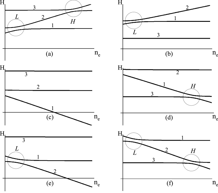
Figure 1: Level crossing diagrams for neutrino flavor conversion in supernova. In neutrino sector there are 2 diagrams which correspond to the normal (a; $\Delta m^{2}_{31}>0$) and the inverted (b; $\Delta m^{2}_{31}<0$) hierarchies. In antineutrino sector there are 4 diagrams which correspond to the normal (c, e; $\Delta m^{2}_{31}>0$) and the inverted (d, f; $\Delta m^{2}_{31}<0$) hierarchies, each doubled by two patterns of small mass splittings, the reactor-normal (c and d; $\Delta\bar{m}^{2}_{21}>0$) the reactor-inverted (e and f; $\Delta\bar{m}^{2}_{21}<0$) hierarchies. In CPT invariant case the diagrams (a) to (d) remain.

The $\nu_{e}$ and $\bar{\nu}_{e}$ survival probabilities $p$ and $\bar{p}$’s are given as

$$p_{N} = |U_{e1}|^{2}P_{H}P_{L}+|U_{e2}|^{2}P_{H}(1-P_{L})+|U_{e3}|^{2}(1-P_{H})$$ (18)

$$\bar{p}_{N21} = |\bar{U}_{e1}|^{2}$$ (19)

$$\bar{p}_{N12} = |\bar{U}_{e1}|^{2}\bar{P}_{L}+|\bar{U}_{e2}|^{2}(1-\bar{P}_{L})$$ (20)

for the normal hierarchy and

$$p_{I} = |U_{e1}|^{2}P_{L}+|U_{e2}|^{2}(1-P_{L})~{}~{}.$$ (21)

$$\bar{p}_{I21} = |\bar{U}_{e1}|^{2}\bar{P}_{H}+|\bar{U}_{e3}|^{2}(1-\bar{P}_{H})$$ (22)

$$\bar{p}_{I12} = |\bar{U}_{e1}|^{2}\bar{P}_{H}\bar{P}_{L}+|\bar{U}_{e2}|^{2}\bar{P}_{H}(1-\bar{P}_{L})+|\bar{U}_{e3}|^{2}(1-\bar{P}_{H})$$ (23)

for the inverted hierarchy.

We note that $\Delta m^{2}_{21}$ and $\bar{\Delta m^{2}}_{21}$ are both in the “LMA” region; The former is constrained to be in the region $2\times 10^{-5}\mbox{eV}^{2}<\Delta m^{2}_{21}<2\times 10^{-4}\mbox{eV}^{2}$ by all the solar neutrino experiments while the latter is $10^{-5}\mbox{eV}^{2}<\bar{\Delta m^{2}}_{21}<2\times 10^{-4}\mbox{eV}^{2}$ by the KamLAND experiments, both at 3 $\sigma$ CL. Then, one can argue quite safely that the L level crossings are adiabatic not only in the neutrino but also in the antineutrino channels, $P_{L}=\bar{P}_{L}=0$. Then, the survival factors take simple forms

$$p_{N} = |U_{e2}|^{2}P_{H}+|U_{e3}|^{2}(1-P_{H})$$ (24)

$$\bar{p}_{N21} = |\bar{U}_{e1}|^{2}$$ (25)

$$\bar{p}_{N12} = |\bar{U}_{e2}|^{2}$$ (26)

for the normal hierarchy and

$$p_{I} = |U_{e2}|^{2}$$ (27)

$$\bar{p}_{I21} = |\bar{U}_{e1}|^{2}\bar{P}_{H}+|\bar{U}_{e3}|^{2}(1-\bar{P}_{H})$$ (28)

$$\bar{p}_{I12} = |\bar{U}_{e2}|^{2}\bar{P}_{H}+|\bar{U}_{e3}|^{2}(1-\bar{P}_{H})$$ (29)

for the inverted hierarchy. Therefore, the distinction between $\Delta\bar{m}^{2}_{21}>0$ and $\Delta\bar{m}^{2}_{21}<0$ cases is just interchanging $|\bar{U}_{e1}|$ and $|\bar{U}_{e2}|$, as expected.

We make a short remarks on possible roles played by the earth matter effect dighe-smi . It is well known that if the H resonance is adiabatic it plays no role. In the case of non-adiabatic H resonance, it can play a role but again it is suppressed by the factor $(2Ea_{\text{earth}}/\Delta m^{2}_{31})\sin^{2}2\theta_{13}$, where $a=\sqrt{2}G_{F}N_{e}(x)$ is related with neutrino’s index of refraction in matter with $G_{F}$ and $N_{e}$ being the Fermi constant and the electron number density, respectively. An explicit computation reveals that the effects of the earth matter effect is small, and moreover it cannot lift the degeneracy between the CPT-conserving and CPT-violating cases. Therefore, we do not discuss it further in the present paper.

IV.2 General Classification of Patterns of Supernova Neutrino Spectra

In the rest of this paper, we focus on the cases in which the H level crossing is completely adiabatic or non-adiabatic; We do not discuss the intermediate case in which the H level crossing is admixture of adiabatic and non-adiabatic transitions. By doing so we restrict ourselves to the two regions of $\theta_{13}$, roughly speaking, $s^{2}_{13}\geq 10^{-4}$ (adiabatic), or $s^{2}_{13}\leq 10^{-6}$ (non-adiabatic). We can classify the possible situation into $4\times 8=32$ cases depending upon

• neutrino and antineutrino mass patterns are either normal or inverted, and if $\Delta\bar{m}^{2}_{21}>0$ or $\Delta\bar{m}^{2}_{21}<0$ in the antineutrino sector

• the H level crossings in neutrino and antineutrino sectors are adiabatic or non-adiabatic,

as given in Table 1. In each case, the neutrino fluxes $F_{e}$, $F_{\bar{e}}$, and $F_{x}$ at a detector can be predicted for a given set of $F_{e}^{0}$, $F_{\bar{e}}^{0}$, and $F_{x}^{0}$ at neutrino sphere.

$\nu$/$\bar{\nu}$ survival factor	$p_{N}$	$p_{I}$	$\bar{p}_{N21}$	$\bar{p}_{N12}$	$\bar{p}_{I21}$	$\bar{p}_{I12}$
Adiabaticity
Adiabatic H crossing	$|U_{e3}|^{2}$	$|U_{e2}|^{2}$	$|\bar{U}_{e1}|^{2}$	$|\bar{U}_{e2}|^{2}$	$|\bar{U}_{e3}|^{2}$	$|\bar{U}_{e3}|^{2}$
Nonadiabatic H crossing	$|U_{e2}|^{2}$	$|U_{e2}|^{2}$	$|\bar{U}_{e1}|^{2}$	$|\bar{U}_{e2}|^{2}$	$|\bar{U}_{e1}|^{2}$	$|\bar{U}_{e2}|^{2}$

Table 1: The electron neutrino and antineutrino survival factors $p$ and $\bar{p}$ are presented for adiabatic and nonadiabatic H level crossings. Note that the apparent duplication due to the adiabatic and non-adiabatic H level crossing in the columns of $p_{I}$, $\bar{p}_{N21}$, and $\bar{p}_{N12}$ are superficial for flavor conversion in supernova because of no H level crossing.

From the viewpoint of neutrino flavor transformation, however, there are enormous degeneracies in the 32 cases. First of all, the duplication due to the adiabatic and non-adiabatic H level crossing in the columns of $p_{I}$, $\bar{p}_{N21}$, and $\bar{p}_{N12}$ (Fig. 1b, Fig. 1c, Fig. 1e) are superficial because of no H level crossing. In fact, one can show from Table 1 that there are only 6 different patterns of the neutrino spectra;

$$P_{31}:p = |U_{e3}|^{2},\bar{p}=|\bar{U}_{e1}|^{2}$$

$$P_{23}:p = |U_{e2}|^{2},\bar{p}=|\bar{U}_{e3}|^{2}$$

$$P_{21}:p = |U_{e2}|^{2},\bar{p}=|\bar{U}_{e1}|^{2}$$

$$P_{32}:p = |U_{e3}|^{2},\bar{p}=|\bar{U}_{e2}|^{2}$$

$$P_{33}:p = |U_{e3}|^{2},\bar{p}=|\bar{U}_{e3}|^{2}$$

$$P_{22}:p = |U_{e2}|^{2},\bar{p}=|\bar{U}_{e2}|^{2}$$ (30)

Each pattern contains several cases of $\nu$ and $\bar{\nu}$ mass hierarchies and (non-)adiabaticity of H resonance. Notice, however, that all the 32 cases must be treated as different scenarios from particle physics point of view. Despite degeneracies in the features of flavor conversion, each of the degenerate scenarios sometimes has different CPT transformation properties.

We use abbreviated notation to represent them. For example, $(\nu:\text{N-AD},\bar{\nu}:\text{I-NAD})$ implies that neutrinos have the normal mass hierarchy and the adiabatic H level crossing, and antineutrinos have the inverted mass hierarchy and the nonadiabatic H level crossing. Then, the content of each flux pattern is:

$$P_{31}: (\nu:\text{N-AD},\bar{\nu}:\text{N21-AD}),\underline{(\nu:\text{N-AD},\bar{\nu}:\text{N21-NAD})},\underline{(\nu:\text{N-AD},\bar{\nu}:\text{I21-NAD})}$$

$$P_{23}: \underline{(\nu:\text{N-NAD},\bar{\nu}:\text{I21-AD})},\underline{(\nu:\text{N-NAD},\bar{\nu}:\text{I12-AD})},(\nu:\text{I-AD},\bar{\nu}:\text{I21-AD}),$$

$$\underline{(\nu:\text{I-AD},\bar{\nu}:\text{I12-AD})},\underline{(\nu:\text{I-NAD},\bar{\nu}:\text{I21-AD})},\underline{(\nu:\text{I-NAD},\bar{\nu}:\text{I12-AD})}$$

$$P_{21}: \underline{(\nu:\text{N-NAD},\bar{\nu}:\text{N21-AD})},(\nu:\text{N-NAD},\bar{\nu}:\text{N21-NAD}),\underline{(\nu:\text{N-NAD},\bar{\nu}:\text{I21-NAD})},$$

$$\underline{(\nu:\text{I-AD},\bar{\nu}:\text{N21-AD})},\underline{(\nu:\text{I-AD},\bar{\nu}:\text{N21-NAD})},\underline{(\nu:\text{I-AD},\bar{\nu}:\text{I21-NAD})},$$

$$\underline{(\nu:\text{I-NAD},\bar{\nu}:\text{N21-AD})},\underline{(\nu:\text{I-NAD},\bar{\nu}:\text{N21-NAD})},(\nu:\text{I-NAD},\bar{\nu}:\text{I21-NAD}),$$

$$P_{32}: \underline{(\nu:\text{N-AD},\bar{\nu}:\text{N12-AD})},\underline{(\nu:\text{N-AD},\bar{\nu}:\text{N12-NAD})},\underline{(\nu:\text{N-AD},\bar{\nu}:\text{I12-NAD})}$$

$$P_{33}: \underline{(\nu:\text{N-AD},\bar{\nu}:\text{I21-AD})},\underline{(\nu:\text{N-AD},\bar{\nu}:\text{I12-AD})}$$

$$P_{22}: \underline{(\nu:\text{N-NAD},\bar{\nu}:\text{N12-AD})},\underline{(\nu:\text{N-NAD},\bar{\nu}:\text{N12-NAD})},\underline{(\nu:\text{N-NAD},\bar{\nu}:\text{I12-NAD})},$$ (31)

$$\underline{(\nu:\text{I-AD},\bar{\nu}:\text{N12-AD})},\underline{(\nu:\text{I-AD},\bar{\nu}:\text{N12-NAD})},\underline{(\nu:\text{I-AD},\bar{\nu}:\text{I12-NAD})},$$

$$\underline{(\nu:\text{I-NAD},\bar{\nu}:\text{N12-AD})},\underline{(\nu:\text{I-NAD},\bar{\nu}:\text{N12-NAD})},\underline{(\nu:\text{I-NAD},\bar{\nu}:\text{I12-NAD})},$$

where the one with (without) underline indicates the case with (without) CPT violation. Several immediate comments are in order; Most notably, only the CPT violating cases are involved in the latter three patterns $P_{32}$, $P_{33}$ and $P_{22}$. Whereas the first three patterns $P_{31}$, $P_{23}$ and $P_{21}$ contain CPT conserving as well as violating cases; There are only 4 CPT conserving cases, two in $P_{21}$, and one in each of $P_{23}$ and in $P_{31}$, and the remaining 28 cases are CPT violating.

Therefore, if one is able to disentangle the latter three patterns observationally, the future supernova neutrino detection has a potential to discover CPT violation. We will discuss this possibility further in the subsequent sections. In the rest of the patterns $P_{21}$, $P_{23}$ and $P_{31}$, with coexistence of CPT violating and CPT conserving cases, observation of supernova neutrinos by itself cannot signal CPT violation nor prove CPT invariance. However, there are possibilities that one can make stronger cases with the help of terrestrial experiments as we discuss in the next section.

V Case of reduced degeneracy with help of other types of experiments

There are several cases in which CPT violation can be signaled more easily by combining SN $\nu$ and $\bar{\nu}$ observation with some other experiments. It occurs in particular in the case that the next generation accelerator JPARC ; NOVA ; SPL ; beta and/or the reactor experiments reactor are able to measure $\theta_{13}$, or go down to the sensitivity to establish non-adiabatic H level crossing nufact . At the stage, it may be possible that some experiments can determine the neutrino mass hierarchy. For recent discussions, see e.g., recent . We explore in this section what would be the effect of these additional inputs for uncovering CPT violation. We do not discuss the cases in which CPT violation is already obvious by these additional informations, for example, the cases such as normal neutrino and inverted antineutrino mass hierarchies, or the measured values of $\theta_{ij}$ and $\bar{\theta}_{ij}$ differ with each other at a high confidence level.

V.1 Detection of $\theta_{13}$ in reactor and accelerator experiments

If the next generation accelerator experiments and/or the reactor measurement succeed to detect the effect of non-vanishing $\theta_{13}$ and $\bar{\theta}_{13}$, respectively, it means that $P_{H}=\bar{P}_{H}=0$. Then, the degeneracy shrinks enormously. In each pattern of masses and level crossings, the cases which remain are:

$$P_{31}: (\nu:\text{N-AD},\bar{\nu}:\text{N21-AD}),$$

$$P_{23}: (\nu:\text{I-AD},\bar{\nu}:\text{I21-AD}),\underline{(\nu:\text{I-AD},\bar{\nu}:\text{I12-AD})},$$

$$P_{21}: \underline{(\nu:\text{I-AD},\bar{\nu}:\text{N21-AD})},$$

$$P_{32}: \underline{(\nu:\text{N-AD},\bar{\nu}:\text{N12-AD})},$$

$$P_{33}: \underline{(\nu:\text{N-AD},\bar{\nu}:\text{I21-AD})},\underline{(\nu:\text{N-AD},\bar{\nu}:\text{I12-AD})},$$

$$P_{22}: \underline{(\nu:\text{I-AD},\bar{\nu}:\text{N12-AD})}.$$ (32)

Novel feature of (32) is that the patterns $P_{21}$ and $P_{31}$ now contain only the CPT violating and CPT conserving cases, respectively. In this case it is sufficient to exclude the patterns $P_{23}$ and $P_{31}$ to establish CPT violation.

V.2 No signal of $\theta_{13}$ in future terrestrial experiments

Suppose that, instead of positive detection which was assumed in the above, no indication for nonzero $\theta_{13}$ and $\bar{\theta}_{13}$ is obtained by the next generation accelerator and reactor experiments. If it continues to be true to the extreme sensitivity reachable by neutrino factory, it would imply that $P_{H}=\bar{P}_{H}=1$. Then, the degeneracy again decreases enormously, but in a quite different way of adiabatic $H$ resonances,

$$P_{21}: (\nu:\text{N-NAD},\bar{\nu}:\text{N21-NAD}),\underline{(\nu:\text{N-NAD},\bar{\nu}:\text{I21-NAD})},$$

$$\underline{(\nu:\text{I-NAD},\bar{\nu}:\text{N21-NAD})},(\nu:\text{I-NAD},\bar{\nu}:\text{I21-NAD}),$$

$$P_{22}: \underline{(\nu:\text{N-NAD},\bar{\nu}:\text{N12-NAD})},\underline{(\nu:\text{N-NAD},\bar{\nu}:\text{I12-NAD})},$$ (33)

$$\underline{(\nu:\text{I-NAD},\bar{\nu}:\text{N12-NAD})},\underline{(\nu:\text{I-NAD},\bar{\nu}:\text{I12-NAD})},$$

$$\hskip-34.14322ptP_{23},P_{31},P_{32},P_{33}:\text{no case remains}$$

The only two patterns, $P_{21}$ and $P_{22}$ are allowed. Rejection of $P_{21}$ or confirmation of $P_{22}$ implies CPT violation.

V.3 The normal $\nu$ and $\bar{\nu}$ mass hierarchies

If the neutrino and antineutrino mass hierarchies are both normal ($\Delta m^{2}_{31}>0$) and if the value of $\theta_{13}$ is not known, only four flux patterns remain;

$$P_{31}: (\nu:\text{N-AD},\bar{\nu}:\text{N21-AD}),\underline{(\nu:\text{N-AD},\bar{\nu}:\text{N21-NAD})},$$

$$P_{21}: \underline{(\nu:\text{N-NAD},\bar{\nu}:\text{N21-AD})},(\nu:\text{N-NAD},\bar{\nu}:\text{N21-NAD}),$$

$$P_{32}: \underline{(\nu:\text{N-AD},\bar{\nu}:\text{N12-AD})},\underline{(\nu:\text{N-AD},\bar{\nu}:\text{N12-NAD})},$$

$$P_{22}: \underline{(\nu:\text{N-NAD},\bar{\nu}:\text{N12-AD})},\underline{(\nu:\text{N-NAD},\bar{\nu}:\text{N12-NAD})}.$$ (34)

Rejection of the flux patterns $P_{31}$ and $P_{21}$, or confirmation of the patterns $P_{32}$ and $P_{22}$ establishes CPT violation.

V.4 The inverted $\nu$ and $\bar{\nu}$ mass hierarchies

If the neutrino and antineutrino mass hierarchies are both inverted type ($\Delta m^{2}_{31}<0$) and if the value of $\theta_{13}$ is not known, only three flux patterns remain.

$$P_{23}: (\nu:\text{I-AD},\bar{\nu}:\text{I21-AD}),\underline{(\nu:\text{I-AD},\bar{\nu}:\text{I12-AD})},$$

$$\underline{(\nu:\text{I-NAD},\bar{\nu}:\text{I21-AD})},\underline{(\nu:\text{I-NAD},\bar{\nu}:\text{I12-AD})}$$

$$P_{21}: \underline{(\nu:\text{I-AD},\bar{\nu}:\text{I21-NAD})},(\nu:\text{I-NAD},\bar{\nu}:\text{I21-NAD}),$$

$$P_{22}: \underline{(\nu:\text{I-AD},\bar{\nu}:\text{I12-NAD})},\underline{(\nu:\text{I-NAD},\bar{\nu}:\text{I12-NAD})}.$$ (35)

To single out the pattern $P_{22}$ appears to be the easiest way to demonstrate CPT violation.

Under the assumptions made in Secs. V.2, V.3, and V.4, CPT violation, once demonstrated, implies the reactor-inverted antineutrino mass hierarchy, $\bar{m}_{2}<\bar{m}_{1}$. Or, equivalently, $\bar{\theta}_{12}$ is in the dark side. Thus, supernova neutrinos can in principle have sensitivity to the $\bar{\theta}_{12}$ light-side vs. dark-side confusion. Below, we examine the cases of additional inputs combined.

V.5 Adiabatic H resonance and the normal or the inverted mass hierarchies

If the H resonance is adiabatic, and if the neutrino and antineutrino mass hierarchies are both normal only two flux patterns remain;

$$P_{31}: (\nu:\text{N-AD},\bar{\nu}:\text{N21-AD}),$$

$$P_{32}: \underline{(\nu:\text{N-AD},\bar{\nu}:\text{N12-AD})}.$$ (36)

If the H resonance is adiabatic, and if the neutrino and antineutrino mass hierarchies are both inverted the allowed flux pattern is unique

$$P_{23}: (\nu:\text{I-AD},\bar{\nu}:\text{I21-AD}),\underline{(\nu:\text{I-AD},\bar{\nu}:\text{I12-AD})}.$$ (37)

In this case, there is no way of telling whether CPT is violated or not in our method.

V.6 Non-adiabatic H resonance and the normal or the inverted mass hierarchies

If the H resonance is non-adiabatic, distinction between mass hierarchies, normal vs. inverted does not make difference in the allowed flux patterns;

$$P_{21}: (\nu:\text{X-NAD},\bar{\nu}:\text{X21-NAD}),$$

$$P_{22}: \underline{(\nu:\text{X-NAD},\bar{\nu}:\text{X12-NAD})}.$$ (38)

where X can be N (normal) or I (inverted). Note that the two flux patterns are different from (36).

VI Characteristic features of pattern dependent neutrino fluxes

We now discuss the characteristic features of neutrino spectra of $e$, $\bar{e}$, and $x$ flavors in each classified patterns of neutrino flavor transformation in supernova. So far we have formulated, in a generic way, the method for testing CPT violation with supernova neutrinos. In the rest of this paper, we concentrate on testing CPT violation caused by difference between neutrino and antineutrino mass patterns as well as their mixing angles $\theta_{13}$ and $\bar{\theta}_{13}$. We take $\theta_{12}=\bar{\theta}_{12}$ in the following analysis. (Note that all the mixing angles are in the first octant in our convention, and $\theta_{23}$ does not come into play.) In some cases based on the Garching simulation we need enormous accuracies of less than a few % to distinguish between varrious spectral patterns. (See Sec. VII.) In such cases there is no hope of establishing CPT violation if the effects caused by small differences in mixing angle $\theta_{12}$ in $\nu$ and $\bar{\nu}$ sectors and the one from neutrino mass pattern coexist.

Though the current bounds on difference between $\theta_{12}$ and $\bar{\theta}_{12}$ are rather mild ones it is quite possible that the room between them will be tighten up as the KamLAND experiment proceeds. The choice $\theta_{12}=\bar{\theta}_{12}$ could become mandatory if the low-energy solar neutrino measurement nakahata and the dedicated reactor $\bar{\theta}_{12}$ experiments MNTZ ; goswami are both realized.

VI.1 Characteristic features of spectral patterns of neutrino fluxes

To give the readers a feeling if the neutrino spectra that arise in the six different patterns can be distinguished, we give an illustration using a model flux based on Livermore simulation livermore . The parameters that characterize spectral form of the flux are given in Table 3 in Sec. VII, where comparison between results with the other two flux models based on the Garching simulation is carried out. In this subsection we employ the Livermore flux because it is, at least, most suitable for illustrative purpose, having clear differences among spectral shapes of three effective neutrino species, as shown in Fig. 2. We note that the results with the Livermore parameters are very similar to the ones with the pinched Fermi-Dirac distribution used in a vast amount of literatures, e.g., in dighe-smi ; MNTV .

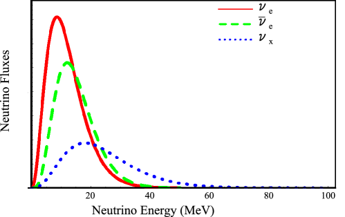
Figure 2: The primary energy spectra of three effective neutrino species $\nu_{e}$ (red solid curve), $\bar{\nu}_{e}$ (green dashed curve), and $\nu_{x}$ (blue dotted curve) of neutrinos just outside the neutrino sphere are shown. The flux model based on the Livermore simulation whose parameters are given in Table 3 in Sec. VII. The absolute normalization is arbitrary.

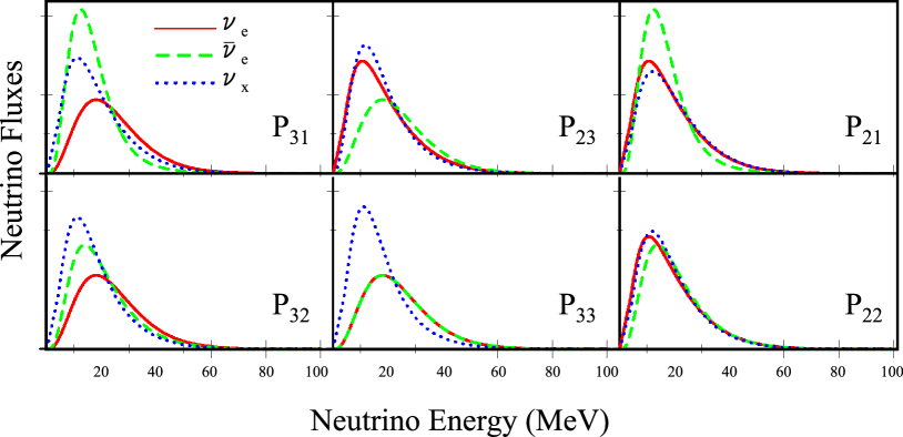
Figure 3: The energy spectra of the three effective neutrino species $\nu_{e}$ (red solid curve), $\bar{\nu}_{e}$ (green dashed curve), and $\nu_{x}$ (blue dotted curve) at terrestrial detectors corresponding to six different patterns of neutrino flavor conversion $P_{31}$ to $P_{22}$ defined in (30) are presented. The Livermore flux model with the same values of parameters as in Fig. 2 is used. Although an over-all absolute normalization is arbitrary, the relative normalization between the six patterns are meaningful.

We draw in Fig. 3 the spectra of the three effective neutrino species $\nu_{e}$, $\bar{\nu}_{e}$, and $\nu_{x}$ of six different patterns of $P_{31}$ to $P_{22}$ defined in (30). One can recognize that the six patterns of neutrino flavor conversion in supernova are quite different with each other partly due to the “optimistic” choice of the parameters. The difference in spectral patterns in three species of neutrinos is the key to discriminate six different scenarios of flavor transformation. For more quantitative understanding, we give in Table 2 the average values of energies $\langle E_{\alpha}\rangle$ ($\alpha=$ e, $\bar{e}$ and x), and the width parameter $\langle\Delta E_{\alpha}\rangle\equiv\sqrt{\langle E_{\alpha}^{2}\rangle-\langle E_{\alpha}\rangle^{2}}$ which is also used in luna-smi2 . To make the distinction among the six patterns clearer we also give in Table 2 the ratios $\langle E_{\beta}\rangle/\langle E_{\bar{e}}\rangle$ and $\langle\Delta E_{\beta}\rangle/\langle\Delta E_{\bar{e}}\rangle$ for $\beta=$ e and x, assuming that the denominators would be the best determined parameters. The distinction among the different flavor conversion pattern is obvious.

Spectral	$\langle E_{e}\rangle$	$\langle E_{\bar{e}}\rangle$	$\langle E_{x}\rangle$	$\langle\Delta E_{e}\rangle$	$\langle\Delta E_{\bar{e}}\rangle$	$\langle\Delta E_{x}\rangle$	$\frac{\langle E_{e}\rangle}{\langle E_{\bar{e}}\rangle}$	$\frac{\langle E_{x}\rangle}{\langle E_{\bar{e}}\rangle}$	$\frac{\langle\Delta E_{e}\rangle}{\langle\Delta E_{\bar{e}}\rangle}$	$\frac{\langle\Delta E_{x}\rangle}{\langle\Delta E_{\bar{e}}\rangle}$
patterns
$P_{31}$	24.0	16.8	18.6	12.0	8.8	11.3	1.43	1.10	1.36	1.29
$P_{23}$	18.7	24.0	18.1	11.6	12.0	10.7	0.78	0.75	0.96	0.89
$P_{21}$	18.7	16.8	19.6	11.6	8.8	11.6	1.11	1.17	1.31	1.32
$P_{32}$	24.0	20.5	17.7	12.0	11.1	10.7	1.17	0.86	1.07	0.96
$P_{33}$	24.0	24.0	17.1	12.0	12.0	10.3	1.0	0.71	1.0	0.86
$P_{22}$	18.7	20.5	17.7	11.6	11.2	12.6	0.91	0.86	1.04	1.13

Table 2: The averaged energies and the width parameters of three species of neutrinos are presented by using the spectra based on the Livermore simulation with the parameters given in Table 3. The upper three patterns, $P_{31}$, $P_{23}$, and $P_{21}$ contain CPT conserving as well as violating cases, whereas the lower three patterns $P_{32}$, $P_{33}$, and $P_{22}$ consist solely of CPT violating ones.

Notice that the upper three patterns, $P_{31}$, $P_{23}$, and $P_{21}$ contain CPT conserving as well as violating cases, whereas the lower three patterns $P_{32}$, $P_{33}$, and $P_{22}$ consist solely of CPT violating ones. Therefore, the above discussion applies, upon restriction to the upper three cases, to the conventional CPT conserving cases as well.

We make comments on some notable features of the results presented in Table 2.

• CPT conserving cases

  It may be instructive to understand the feature of the CPT conserving cases contained in the patterns $P_{31}$, $P_{23}$, and $P_{21}$. In the pattern $P_{31}$ (the case of normal hierarchy and adiabatic H resonance) the H resonance is in the neutrino channel, and $\langle E_{e}\rangle/\langle E_{\bar{e}}\rangle>1$ because $\nu_{e}$ at the terrestrial detector is dominantly composed by $\nu_{x}$ at the neutrinosphere MN90 . In the pattern $P_{23}$ (the case of inverted hierarchy and adiabatic H resonance) the H resonance is in the antineutrino channel, and therefore $\langle E_{e}\rangle/\langle E_{\bar{e}}\rangle<1$. The distinction between $P_{31}$ and $P_{23}$ allows to distinguish the normal and the inverted mass hierarchies MN_inverted . In the pattern $P_{21}$ (the case of non-adiabatic H resonance) $\nu_{e}$ ($\bar{\nu}_{e}$) at the earth are superposition of $\nu_{e}$ ($\bar{\nu}_{e}$) and $\nu_{x}$ at the neutrinosphere. These features are extensively discussed by many authors MN_inverted ; dighe-smi ; dutta ; todai ; MNTV ; barger ; luna-smi1 ; luna-smi2 .

• CPT violating cases

  As one can recognize from Table 2 there is a general tendency that $\langle E_{x}\rangle/\langle E_{\bar{e}}\rangle$ is small in CPT violating cases. Unfortunately, it does not guarantee unique identification of them because of the similar small ratio of $P_{23}$. But the latter has distinctive feature that all the ratios $\langle E_{\alpha}\rangle/\langle E_{\bar{e}}\rangle$ and $\langle\Delta E_{\alpha}\rangle/\langle\Delta E_{\bar{e}}\rangle$ ($\alpha=e,x$) are smaller than unity. The feature may allow unique identification of $P_{23}$, and hence that of CPT violating cases by elimination.

VI.2 Approximate Analytic Expression of the Flux Composition

To facilitate clear understanding and to complement the drawing of figures we give approximate expressions of fluxes. They will help understanding the features of Fig. 3. We use the approximations $s_{13}\ll 1$ and $\bar{s}_{13}\ll 1$ (assuming that the former is true) which are numerically valid. Notice that it does not mean that we restrict to the case of non-adiabatic H-level crossing. The approximation applies to the expressions of fluxes after taking $P_{H}=0$ or $P_{H}=1$ etc. to merely simplify the expressions.

• Pattern $P_{31}$

In this case $p=|U_{e3}|^{2}=s^{2}_{13}$ and $\bar{p}=|\bar{U}_{e1}|^{2}=\bar{c}^{2}_{12}\bar{c}^{2}_{13}$. Then, the $\nu_{e}$, $\bar{\nu}_{e}$, and $\nu_{x}$ spectra are given by:

$$F_{e} = s^{2}_{13}F_{e}^{0}+c^{2}_{13}F_{x}^{0}\approx F_{x}^{0},$$

$$F_{\bar{e}} = \bar{c}^{2}_{12}\bar{c}^{2}_{13}F_{\bar{e}}^{0}+(1-\bar{c}^{2}_{12}\bar{c}^{2}_{13})F_{x}^{0}\approx\bar{c}^{2}_{12}F_{\bar{e}}^{0}+\bar{s}^{2}_{12}F_{x}^{0},$$

$$4F_{x} = c^{2}_{13}F_{e}^{0}+(1-\bar{c}^{2}_{12}\bar{c}^{2}_{13})F_{\bar{e}}^{0}+(2+s^{2}_{13}+\bar{c}^{2}_{12}\bar{c}^{2}_{13})F_{x}^{0}$$ (39)

$$\approx F_{e}^{0}+\bar{s}^{2}_{12}F_{\bar{e}}^{0}+(2+\bar{c}^{2}_{12})F_{x}^{0}.$$

• Pattern $P_{23}$

In this case $p=|U_{e2}|^{2}=s^{2}_{12}c^{2}_{13}$ and $\bar{p}=|\bar{U}_{e3}|^{2}=\bar{s}^{2}_{13}$. Then, the $\nu_{e}$, $\bar{\nu}_{e}$, and $\nu_{x}$ spectra are given by:

$$F_{e} = s^{2}_{12}c^{2}_{13}F_{e}^{0}+(1-s^{2}_{12}c^{2}_{13})F_{x}^{0}\approx s^{2}_{12}F_{e}^{0}+c^{2}_{12}F_{x}^{0},$$

$$F_{\bar{e}} = \bar{s}^{2}_{13}F_{e}^{0}+\bar{c}^{2}_{13}F_{x}^{0}\approx F_{x}^{0},$$

$$4F_{x} = (1-s^{2}_{12}c^{2}_{13})F_{e}^{0}+\bar{c}^{2}_{13}F_{\bar{e}}^{0}+(2+s^{2}_{12}c^{2}_{13}+\bar{s}^{2}_{13})F_{x}^{0}$$ (40)

$$\approx c^{2}_{12}F_{e}^{0}+F_{\bar{e}}^{0}+(2+s^{2}_{12})F_{x}^{0}.$$

• Pattern $P_{21}$

In this case $p=|U_{e2}|^{2}=s^{2}_{12}c^{2}_{13}$ and $\bar{p}=|\bar{U}_{e1}|^{2}=\bar{c}^{2}_{12}\bar{c}^{2}_{13}$. Then, the $\nu_{e}$, $\bar{\nu}_{e}$, and $\nu_{x}$ spectra are given by:

$$F_{e} = s^{2}_{12}c^{2}_{13}F_{e}^{0}+(1-s^{2}_{12}c^{2}_{13})F_{x}^{0}\approx s^{2}_{12}F_{e}^{0}+c^{2}_{12}F_{x}^{0},$$

$$F_{\bar{e}} = \bar{c}^{2}_{12}\bar{c}^{2}_{13}F_{\bar{e}}^{0}+(1-\bar{c}^{2}_{12}\bar{c}^{2}_{13})F_{x}^{0}\approx\bar{c}^{2}_{12}F_{\bar{e}}^{0}+\bar{s}^{2}_{12}F_{x}^{0},$$

$$4F_{x} = (1-s^{2}_{12}c^{2}_{13})F_{e}^{0}+(1-\bar{c}^{2}_{12}\bar{c}^{2}_{13})F_{\bar{e}}^{0}+(2+s^{2}_{12}c^{2}_{13}+\bar{c}^{2}_{12}\bar{c}^{2}_{13})F_{x}^{0}$$ (41)

$$\approx c^{2}_{12}F_{e}^{0}+\bar{s}^{2}_{12}F_{\bar{e}}^{0}+(2+s^{2}_{12}+\bar{c}^{2}_{12})F_{x}^{0}.$$

• Pattern $P_{32}$

This case contains only CPT violating patterns. In this case $p=|U_{e3}|^{2}=s^{2}_{13}$ and $\bar{p}=|\bar{U}_{e2}|^{2}=\bar{s}^{2}_{12}\bar{c}^{2}_{13}$. Then, the $\nu_{e}$, $\bar{\nu}_{e}$, and $\nu_{x}$ spectra are given by:

$$F_{e} = s^{2}_{13}F_{e}^{0}+c^{2}_{13}F_{x}^{0}\approx F_{x}^{0},$$

$$F_{\bar{e}} = \bar{s}^{2}_{12}\bar{c}^{2}_{13}F_{\bar{e}}^{0}+(1-\bar{s}^{2}_{12}\bar{c}^{2}_{13})F_{x}^{0}\approx\bar{s}^{2}_{12}F_{\bar{e}}^{0}+\bar{c}^{2}_{12}F_{x}^{0},$$

$$4F_{x} = c^{2}_{13}F_{e}^{0}+(1-\bar{s}^{2}_{12}\bar{c}^{2}_{13})F_{\bar{e}}^{0}+(2+s^{2}_{13}+\bar{s}^{2}_{12}\bar{c}^{2}_{13})F_{x}^{0}$$ (42)

$$\approx F_{e}^{0}+\bar{c}^{2}_{12}F_{\bar{e}}^{0}+(2+\bar{s}^{2}_{12})F_{x}^{0}.$$

• Pattern $P_{33}$

This case contains only CPT violating patterns. In this case $p=|U_{e3}|^{2}=s^{2}_{13}$ and $\bar{p}=|\bar{U}_{e3}|^{2}=\bar{s}^{2}_{13}$. Then, the $\nu_{e}$, $\bar{\nu}_{e}$, and $\nu_{x}$ spectra are given by:

$$F_{e} = s^{2}_{13}F_{e}^{0}+c^{2}_{13}F_{x}^{0}\approx F_{x}^{0},$$

$$F_{\bar{e}} = \bar{s}^{2}_{13}F_{e}^{0}+\bar{c}^{2}_{13}F_{x}^{0}\approx F_{x}^{0},$$

$$4F_{x} = c^{2}_{13}F_{e}^{0}+\bar{c}^{2}_{13}F_{\bar{e}}^{0}+(2+s^{2}_{13}+\bar{s}^{2}_{13})F_{x}^{0}$$ (43)

$$\approx F_{e}^{0}+F_{\bar{e}}^{0}+2F_{x}^{0}.$$

• Pattern $P_{22}$

This case contains only CPT violating patterns. In this case $p=|U_{e2}|^{2}=s^{2}_{12}c^{2}_{13}$ and $\bar{p}=|\bar{U}_{e2}|^{2}=\bar{s}^{2}_{12}\bar{c}^{2}_{13}$. Then, the $\nu_{e}$, $\bar{\nu}_{e}$, and $\nu_{x}$ spectra are given by:

$$F_{e} = s^{2}_{12}c^{2}_{13}F_{e}^{0}+(1-s^{2}_{12}c^{2}_{13})F_{x}^{0}\approx s^{2}_{12}F_{e}^{0}+c^{2}_{12}F_{x}^{0},$$

$$F_{\bar{e}} = \bar{s}^{2}_{12}\bar{c}^{2}_{13}F_{\bar{e}}^{0}+(1-\bar{s}^{2}_{12}\bar{c}^{2}_{13})F_{x}^{0}\approx\bar{s}^{2}_{12}F_{\bar{e}}^{0}+\bar{c}^{2}_{12}F_{x}^{0},$$

$$4F_{x} = (1-s^{2}_{12}c^{2}_{13})F_{e}^{0}+(1-\bar{s}^{2}_{12}\bar{c}^{2}_{13})F_{\bar{e}}^{0}+(2+s^{2}_{12}c^{2}_{13}+\bar{s}^{2}_{12}\bar{c}^{2}_{13})F_{x}^{0}$$ (44)

$$\approx c^{2}_{12}F_{e}^{0}+\bar{c}^{2}_{12}F_{\bar{e}}^{0}+(2+s^{2}_{12}+\bar{s}^{2}_{12})F_{x}^{0}.$$

VII To What Extent Can Neutrino Flux Patterns Be Discriminated?

In this section, we briefly discuss to what extent the flux patterns predicted by six cases from $P_{31}$ to $P_{22}$ can be discriminated observationally. Our discussion cannot be a quantitative one because of the lack of “standard supernova model” which has comparable accuracies possessed by the standard solar model. But, it may give us a feeling of how accurate should be the flavor-dependent reconstruction of neutrino spectra to discriminate the six different patterns of flavor conversion.

We also address in Sec.VII.3 the question to what extent limiting the number of possible flux patterns by additional inputs help identifying CPT violation.

VII.1 Model dependence of the prediction to flux spectral patterns

To reflect the best knowledges of supernova simulation currently at hand, we employ in this section the parametrization of fluxes which is used by the Garching group to fit their data MKeil ; Keil02 :

$$F^{0}_{\alpha}(E)=\frac{\Phi_{\alpha}}{\langle E_{\alpha}\rangle}\,\frac{\beta_{\alpha}^{\beta_{\alpha}}}{\Gamma(\beta_{\alpha})}\left(\frac{E}{\langle E_{\alpha}\rangle}\right)^{\beta_{\alpha}-1}\exp\left(-\beta_{\alpha}\frac{E}{\langle E_{\alpha}\rangle}\right)\,,$$ (45)

where $\langle E_{\alpha}\rangle$ denotes their average energy, $\beta_{\alpha}$ is a dimensionless parameter which is related to the width of the spectrum and typically takes on values 3.5–6. For definiteness, we assume $\beta_{\nu_{e}}=3.5$, $\beta_{\nu_{x}}=4$, and $\beta_{\bar{\nu}_{e}}=5$. For the sake of comparison and to reveal dependence on supernova simulations we examine the three different sets of parameters, the same ones used in tomas_etal . They are the fluxes obtained from the Livermore simulation livermore , and typical two model fluxes based on simulation done by the Garching group garching . The three model flux parameters are given in Table 3 as L, G1 and G2.

Model	$\langle E_{0}(\nu_{e})\rangle$	$\langle E_{0}(\bar{\nu}_{e})\rangle$	$\langle E_{0}(\nu_{x})\rangle$	$\frac{\Phi_{0}(\nu_{e})}{\Phi_{0}(\nu_{x})}$	$\frac{\Phi_{0}(\bar{\nu}_{e})}{\Phi_{0}(\nu_{x})}$
L	12	15	24	2.0	1.6
G1	12	15	18	0.8	0.8
G2	12	15	15	0.5	0.5

Table 3: The parameters of the primary neutrino spectra models motivated from SN simulations of the Garching (G1, G2) and the Livermore (L) groups, the same as used in tomas_etal . We assume $\beta_{\nu_{e}}=3.5$, $\beta_{\nu_{x}}=4$, and $\beta_{\bar{\nu}_{e}}=5$.

In Fig. 4, the spectra of the three effective neutrino species $\nu_{e}$, $\bar{\nu}_{e}$, and $\nu_{x}$ of six different patterns of $P_{31}$ to $P_{22}$ defined in (30) are plotted by taking model parameters G1 (upper figures) and G2 (lower figures) in Table 3. As one can recognize the six flavor conversion patterns is much harder to distinguish than the case of Livermore flux.

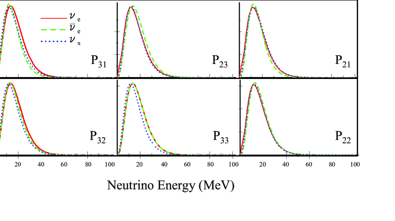
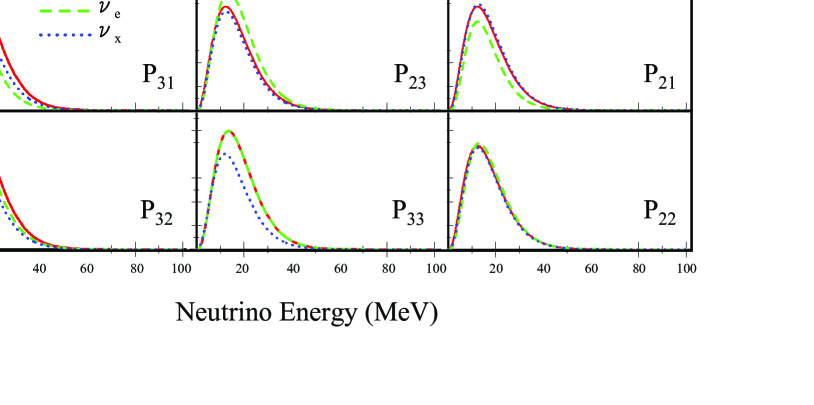
Figure 4: The energy spectra of the three effective neutrino species $\nu_{e}$ (red solid curve), $\bar{\nu}_{e}$ (green dashed curve), and $\nu_{x}$ (blue dotted curve) at terrestrial detectors corresponding to six different patterns of neutrino flavor conversion $P_{31}$ to $P_{22}$ defined in (30) are presented. The Garching flux model parameters G1 (upper figures) and G2 (lower figures) are used.

To obtain a hint on how much accuracy is needed to disentangle these six patterns we give in Table 4 the averaged energies and width parameters of three species of neutrinos as done in Table 2. With the Garching parameters, typically a few % accuracies for the determination of ratios $\langle E_{\alpha}\rangle/\langle E_{\bar{e}}\rangle$ and $\langle\Delta E_{\alpha}\rangle/\langle\Delta E_{\bar{e}}\rangle$ ($\alpha=$ e and x) are required. Whereas in the case of the Livermore parameters, we may be able to do the job with the accuracies of $\sim$10 %.

In addition to these quantities we have added in Table 4 columns for the ratio of luminosity of $\nu_{e}$ and $\nu_{x}$ to $\bar{\nu}_{e}$. (We note that even if the columns are added in Table 2 it is not informative because of the equi-partition of luminosity between three species.) It should not be too difficult to distinguish among the six patterns if the luminosity are measured at the level of a few % level (G1) and 5-10% level (G2).

Spectral	$\langle E_{e}\rangle$	$\langle E_{\bar{e}}\rangle$	$\langle E_{x}\rangle$	$\langle\Delta E_{e}\rangle$	$\langle\Delta E_{\bar{e}}\rangle$	$\langle\Delta E_{x}\rangle$	$\frac{\langle E_{e}\rangle}{\langle E_{\bar{e}}\rangle}$	$\frac{\langle E_{x}\rangle}{\langle E_{\bar{e}}\rangle}$	$\frac{\langle\Delta E_{e}\rangle}{\langle\Delta E_{\bar{e}}\rangle}$	$\frac{\langle\Delta E_{x}\rangle}{\langle\Delta E_{\bar{e}}\rangle}$	$\frac{\langle L_{e}\rangle}{\langle L_{\bar{e}}\rangle}$	$\frac{\langle L_{x}\rangle}{\langle L_{\bar{e}}\rangle}$
patterns
$P_{31}$	18.0	16.0	16.5	9.0	7.7	8.7	1.12	1.03	1.17	1.13	1.31	1.13
$P_{23}$	16.5	18.0	16.4	8.8	9.0	8.5	0.92	0.91	0.98	0.94	0.87	0.83
$P_{21}$	16.5	16.0	16.9	8.8	7.7	8.8	1.03	1.06	1.15	1.15	1.14	1.17
$P_{32}$	18.0	17.3	16.2	9.0	8.6	8.5	1.04	0.94	1.05	0.99	1.11	0.91
$P_{33}$	18.0	18.0	16.0	9.0	8.4	8.4	1.0	0.89	1.0	0.93	1.0	0.80
$P_{22}$	16.5	17.3	16.9	8.8	8.6	8.1	0.96	0.98	1.03	0.94	0.96	0.95

Spectral	$\langle E_{e}\rangle$	$\langle E_{\bar{e}}\rangle$	$\langle E_{x}\rangle$	$\langle\Delta E_{e}\rangle$	$\langle\Delta E_{\bar{e}}\rangle$	$\langle\Delta E_{x}\rangle$	$\frac{\langle E_{e}\rangle}{\langle E_{\bar{e}}\rangle}$	$\frac{\langle E_{x}\rangle}{\langle E_{\bar{e}}\rangle}$	$\frac{\langle\Delta E_{e}\rangle}{\langle\Delta E_{\bar{e}}\rangle}$	$\frac{\langle\Delta E_{x}\rangle}{\langle\Delta E_{\bar{e}}\rangle}$	$\frac{\langle L_{e}\rangle}{\langle L_{\bar{e}}\rangle}$	$\frac{\langle L_{x}\rangle}{\langle L_{\bar{e}}\rangle}$
patterns
$P_{31}$	15.0	15.0	14.6	7.5	7.1	7.4	1.0	0.97	1.06	1.05	1.56	1.27
$P_{23}$	14.5	15.0	14.7	7.4	7.5	7.3	0.97	0.98	0.99	0.98	0.83	0.77
$P_{21}$	14.5	15.0	14.7	7.4	7.1	7.4	0.97	0.98	1.05	1.05	1.29	1.33
$P_{32}$	15.0	15.0	14.5	7.5	7.4	7.3	1.0	0.97	1.02	0.99	1.17	0.89
$P_{33}$	15.0	15.0	14.5	7.5	7.5	7.3	1.0	0.97	1.0	0.97	1.0	0.73
$P_{22}$	14.5	15.0	15.3	7.4	7.4	5.9	0.97	1.02	1.01	0.79	0.97	0.94

Table 4: The same as in Table 2 but with the flux models G1 (upper table) and G2 (lower table) based on the Garching simulation with the parameters given in Table 3. Two extra columns for luminosity ratios are added.

VII.2 How accurately can the supernova neutrino fluxes be determined?

To give the readers some feeling we give a brief remark on how accurately determination of the supernova neutrino fluxes can be done in future observation of galactic supernovae. We must emphasize that the method for such flux reconstruction, which is of great importance solely from the supernova core diagnostics independent of testing CPT symmetry, is not yet developed to a sufficient level. It is the important problem that deserves thorough study to identify a minimal set of detectors which are capable of reconstructing fluxes which can watch supernova for a long run of at least $\sim$50 years.

Lacking such studies we restrict ourselves to accuracy expected for parameters determinable with $\bar{\nu}_{e}$ observation in water Cherenkov detectors. In MNTV it was found that the parameters of the primary flux $\langle E_{\bar{e}}\rangle$ and $\tau_{E}\equiv\langle E_{x}\rangle/\langle E_{\bar{e}}\rangle$ can be determined to the accuracies 1% (4%) and 1.5% (9%) at 3 $\sigma$ CL with Hyper-Kamiokande nakamura (Super-Kamiokande), respectively. The accuracies found in MNTV correspond to the ones of primary fluxes but we here assume that the similar accuracies can be expected for the terrestrial fluxes. If these accuracies can be extended to $\nu_{e}$ flux (which is, however, highly nontrivial) it may be possible to disentangle the flux patterns expected in the six different patterns of flavor conversion. We stress that though the accuracy required for flux determination for identifying CPT violation is quite a demanding one, they are at the same level as that required to diagnose interior of supernova core by means of neutrinos.

VII.3 How additional inputs from accelerator and reactor experiments help identifying CPT violation?

In Sec. V we have discussed which flux patterns will remain if the next generation accelerator and reactor experiments measure $\theta_{13}$ and $\bar{\theta}_{13}$ and/or determine the $\nu$ and $\bar{\nu}$ mass hierarchies. We discuss in this subsection how the reduction of numbers of possible flux patterns help to discriminate between CPT invariant and non-invariant cases.

If the H level crossing is non-adiabatic, the two flux patterns $P_{21}$ and $P_{22}$ remain. In fact, it is the general feature of the non-adiabatic H level crossing, independent of mass hierarchy, as we have seen in Sec. V.2. In the Garching flux model G1, the ratios of average neutrino energies and the widths of energy distributions of $\nu_{e}$ and $\nu_{x}$ to $\bar{\nu}_{e}$ are higher by about 7 - 20% in the flux pattern $P_{21}$ than in $P_{22}$. At the same time, the luminosity ratios are higher in $P_{21}$ by about 20%. In the model G2, the luminosity ratios are again higher by 30-40% in the flux pattern $P_{21}$ than in $P_{22}$. The average energy and width ratios do not differ much except for $\frac{\langle\Delta E_{x}\rangle}{\langle\Delta E_{\bar{e}}\rangle}$ in which it is higher by about 30% in $P_{21}$.

If the H level crossing is adiabatic the results depend upon the $\nu$ and $\bar{\nu}$ mass hierarchies. If they are both normal we are left with two flux patterns $P_{31}$ and $P_{32}$ (Sec. V.5). In the Garching flux model G1, all the four ratios of average neutrino energies and their widths of the flux patterns $P_{31}$ are higher by about 10% than those of $P_{32}$. The luminosity ratios also differ by about 20%. In the model G2, average energy and width ratios do not show any appreciable difference, but the luminosity ratios are higher by 30-40% in the flux pattern $P_{31}$ than in $P_{32}$. If the $\nu$ and $\bar{\nu}$ mass hierarchies are both inverted there is no way of signaling CPT violation in our method.

Therefore, it appears that there is a chance to uncover CPT violation within the accuracy which may be expected in a future detectors. Of course, we should not rely too much on the particular set of flux models to judge to what extent the different flux patterns are discriminable. But, the examination we have gone through in the above suggests that there are some possibilities of uncovering CPT violation by our method at least under circumstances helped by future terrestrial measurement.

VII.4 Supernova model dependence

Here, we want to give a cautionary remark. Uncovering CPT violation along the way we discussed in this paper can only be claimed on the ground that the supernova simulations at the time of observation are reliable to certain extent. Even in the luckiest case in which we know the mass hierarchy and that $\theta_{13}$ is in a region measurable by the next generation reactor and accelerator search, we need credibility in the flux model, roughly speaking, to 10-20% level in the predictions to the ratios of average energy, width, and the luminosity of $\nu_{e}$ and $\nu_{x}$ to $\bar{\nu}_{e}$.

Suppose that a future measurement of supernova neutrino flux strongly suggest CPT violation by preferring one (or more) of the flux patterns which consists only of CPT violating mass patterns, or by disfavoring any of the CPT invariant patterns. Then, one is tempted to conclude that CPT violation is signaled. The point is that the conclusion can be made firmer only by calibrating supernova simulation by accumulation of data gained by many explosions for consistency check. This point is a inherent weakness of the method of signaling CPT violation by supernova neutrino data. We want to emphasize, however, that it is quite thinkable that we will have reliable model simulation of explosion in a timely way, by which neutrino flux can be predicted with high accuracies. Neutrinos are the main engine of the explosion (they are like the pp neutrinos in the Sun) and, most probably, only the ordinary known physics is involved inside the core.

VII.5 Implications to analyses with CPT invariance

As we mentioned at the end of Sec. I, part of the formulas and the analysis in this paper contain some informations useful for conventional analysis with CPT, in particular in the context of flavor-dependent reconstruction of three fluxes. We mention only a few points below, leaving full exposition to possible future works.

Look at the analytic formulas (39) and (40) in Sec. VI.2. From these equations, we notice the following features: In (39) which applies to the case of normal mass hierarchy with adiabatic H resonance, the primary $\nu_{e}$ spectrum does not show up (or has a suppression factor of $s_{13}^{2}$) in the $\nu_{e}$ and $\bar{\nu}_{e}$ spectra observed at the terrestrial detectors. It means that to reconstruct the primary $\nu_{e}$ spectrum accurate measurement of $\nu_{x}$ spectrum together with those of $\nu_{e}$ and $\bar{\nu}_{e}$ is mandatory. Similarly, the primary $\bar{\nu}_{e}$ spectrum does not appear (or has a suppression factor of $s_{13}^{2}$) in the $\nu_{e}$ and $\bar{\nu}_{e}$ spectra in (40) which applies to the case of inverted mass hierarchy with adiabatic H resonance.

In these two cases it would be very difficult to reconstruct the primary $\nu_{e}$ ($\bar{\nu}_{e}$) spectrum in the case of normal (inverted) mass hierarchy with adiabatic H resonance, because spectral measurement of $\nu_{x}$ is difficult. (See, however, beacom for a possible way out.) We believe that it is one of the crucial problems in the program of flavor-dependent reconstruction of primary neutrino fluxes in the interior of supernova.

The case of normal and inverted mass hierarchies with non-adiabatic H resonance, (41), may be the easiest one, relatively speaking, among the three CPT conserving patterns. It is because spectral measurement of $\bar{\nu}_{e}$ and $\nu_{e}$ (if possible) would allow us to determine all the three primary fluxes if the separation of two Fermi-Dirac type distributions with different temperatures is possible, as illustrated in MNTV .

VIII Concluding remarks

We have discussed a method of using neutrinos from supernova to test CPT symmetry. Because of the possibility of having mass and mixing patterns of antineutrinos which can be different from neutrinos 32 different scenarios are allowed which differ in neutrino mass patterns and (non-) adiabaticity of high-density resonance. They produce six different patterns of supernova neutrino energy spectra at the terrestrial neutrino detectors, apart from small modification due to earth matter effect. Among the six patterns, three of them contain only the CPT violating cases. Even in the mixed cases of CPT invariance and violation additional input on the values of $\theta_{13}$ from reactor and accelerator experiments further enhance the possibility of identifying CPT violation.

Future galactic supernovae watched by arrays of massive detectors may allow flavor-dependent reconstruction of three species of neutrino spectra, $\nu_{e}$, $\bar{\nu}_{e}$ and $\nu_{x}$ (a collective notation for $\nu_{\mu}$, $\bar{\nu}_{\mu}$, $\nu_{\tau}$, and $\bar{\nu}_{\tau}$). Assuming capability of obtaining such the informations, which are also required to diagnose supernova core in conventional analysis with CPT, we have shown that one of the three CPT violating patterns may be singled out observationally. The help by the other measurement of lepton mixing parameters by reactor and accelerator experiments would help to identify CPT violating cases. Thus, we have shown that supernova neutrino can be a powerful tool to detect possible gross violation of CPT symmetry such as different mass patterns of neutrinos and antineutrinos. We emphasize the potential power of the method; It may allow to disentangle different (1-3) and (1-2) mass hierarchies both in neutrino and antineutrino sectors in a single “bang”.

However, we also noticed the weakness of the method. We have just mentioned the flux model dependence in the previous section. Another drawback of the method concerns with its weakness at the precision test. In this paper, we have focused on the possibility of detecting CPT violation through identifying unequal mass patterns in neutrino and antineutrino sectors. If the two CPT violation in masses as well as mixing angles coexist, however, it would be very difficult to clearly distinguish the six different patterns of neutrino flavor conversion, the topics we are unable to address in this paper. Therefore, it is important to have stringent bound on difference between neutrino and antineutrino mixing angles in order for the supernova method for testing CPT to work. Similarly, the analysis would be very complicated if $\theta_{13}$ is in the intermadiate region between adiabatic and non-adiabatic H resonance.

Suppose that CPT violation is signaled with supernova neutrinos in the way described in this paper. Then, one may feel that the confirmation by using man made neutrino beam necessary because of the fundamental importance of CPT symmetry. Then, the question is; Is it possible to confirm CPT violation by the alternative methods? Fortunately, the answer is yes. The possibility of using two detectors at the different baseline with $\nu$ beam only (not $\bar{\nu}$) to determine the neutrino mass hierarchy is proposed some time ago nu-nu . Therefore, hypothesis of different mass hierarchies of neutrinos and antineutrinos can, in principle, be tested by separate measurement using the $\pi^{+}$ and $\pi^{-}$ beams. Determining the sign of $\Delta m^{2}_{21}$ in antineutrino sector is harder to carry out, as discussed in gouvea . In any way, distinguishing neutrino mass hierarchy is a very challenging experiment and large-scale apparatus is required. We emphasize, therefore, that indication of CPT violation given by supernova neutrinos can give a good starting point of vital search for the totally unexpected phenomenon of CPT violation.