UCSD-PTH 05-08

TUM-HEP-585/05

ROMA-1404/05

hep-ph/0505110

Upper Bounds on Rare $K$ and $B$ Decays from Minimal Flavour Violation

Christoph Bobeth,^a Marcella Bona,^b Andrzej J. Buras,^c
Thorsten Ewerth,^d Maurizio Pierini,^e Luca Silvestrini,^c,f
and Andreas Weiler^c

^a Physics Department, University of California at San Diego, La Jolla, CA 92093, USA

^b Dipartimento di Fisica, Università di Torino and INFN, Sezione di Torino, Via P. Giuria 1, I-10125 Torino, Italy

^c Physik Department, Technische Universität München, D-85748 Garching, Germany

^d Institute of Theoretical Physics, Sidlerstrasse 5, CH-3012 Bern, Switzerland

^e Laboratoire de l’Accélérateur Linéaire, IN2P3-CNRS et Université de Paris-Sud, BP 34, F-91898 Orsay Cedex

^f Dipartimento di Fisica, Università di Roma “La Sapienza” and INFN, Sezione di Roma, Piazzale A. Moro 2, 00185 Roma, Italy

We study the branching ratios of rare $K$ and $B$ decays in models with minimal flavour violation, using the presently available information from the universal unitarity triangle analysis and from the measurements of $Br(B\to X_{s}\gamma)$, $Br(B\to X_{s}l^{+}l^{-})$ and $Br(K^{+}\rightarrow\pi^{+}\nu\bar{\nu})$. We find the following upper bounds: $Br(K^{+}\rightarrow\pi^{+}\nu\bar{\nu})<11.9\times 10^{-11}$, $Br(K_{\rm L}\rightarrow\pi^{0}\nu\bar{\nu})<4.6\times 10^{-11}$, $Br(K_{\rm L}\to\mu^{+}\mu^{-})_{\mathrm{S}D}<1.4\times 10^{-9}$, $Br(B\to X_{s}\nu\bar{\nu})<5.2\times 10^{-5}$, $Br(B\to X_{d}\nu\bar{\nu})<2.2\times 10^{-6}$, $Br(B_{s}\to\mu^{+}\mu^{-})<7.4\times 10^{-9}$, $Br(B_{d}\to\mu^{+}\mu^{-})<2.2\times 10^{-10}$ at $95\%$ probability. We analyze in detail various possible scenarios with positive or negative interference of Standard Model and New Physics contributions, and show how an improvement of experimental data corresponding to the projected 2010 B factory integrated luminosities will allow to disentangle and test these different possibilities. Finally, anticipating that subsequently the leading role in constraining this kind of new physics will be taken over by the rare decays $K^{+}\rightarrow\pi^{+}\nu\bar{\nu}$, $K_{\rm L}\rightarrow\pi^{0}\nu\bar{\nu}$ and $B_{s,d}\to\mu^{+}\mu^{-}$, that are dominated by the $Z^{0}$-penguin function $C$, we also present plots for several branching ratios as functions of $C$. We point out an interesting triple correlation between $K^{+}\to\pi^{+}\nu\bar{\nu}$, $B\to X_{s}\gamma$ and $B\to X_{s}l^{+}l^{-}$ present in MFV models.

1 Introduction

Recently, great experimental progress has been made in the study of Flavour Changing Neutral Current (FCNC) decays, leading not only to an impressive accuracy in the extraction of CKM parameters from the Unitarity Triangle (UT) analysis [1, 2], but also to stringent constraints on models with extra sources of flavour and CP violation, although an accidental agreement of the UT analysis with the Standard Model (SM) cannot yet be excluded [3, 4].

One is then naturally led to consider models with Minimal Flavour Violation (MFV) [5], in which flavour and CP violation is governed entirely by the CKM matrix [6, 7] and the relevant operators in effective Hamiltonians for weak decays are the same as in the SM.

As pointed out in [5], there exists a universal unitarity triangle (UUT) valid in all these models, that can be constructed independently of the parameters specific to a given model. Moreover, there exist several relations between various branching ratios that allow straightforward tests of these models. A review has been given in [8].

This formulation of MFV agrees with the one of [9, 10] except for the case of models with two Higgs doublets at large $\tan\beta$, where also additional operators, strongly suppressed in the SM, can contribute significantly and the relations in question are not necessarily satisfied. In the present paper, MFV will be defined as in [5, 8].

As reviewed in [8], this class of models can be formulated to a very good approximation in terms of eleven parameters: four parameters of the CKM matrix and seven values of the universal master functions $F_{i}(v)$ that parametrize the short distance contributions to rare decays with $v$ denoting symbolically the parameters of a given MFV model. However, as argued in [8], the new physics contributions to the functions

$$S(v),\qquad C(v),\qquad D^{\prime}(v),$$ (1.1)

representing respectively $\Delta F=2$ box diagrams, $Z^{0}$-penguin diagrams and the magnetic photon penguin diagrams, are the most relevant ones for phenomenology, with the remaining functions producing only minor deviations from the SM in low-energy processes. Several explicit calculations within models with MFV confirm this conjecture. We have checked the impact of these additional functions on our analysis, and we will comment on it in Section 3.

Now, the existence of a UUT implies that the four CKM parameters can be determined independently of the values of the functions in (1.1). Moreover, only $C(v)$ and $D^{\prime}(v)$ enter the branching ratios for radiative and rare decays so that constraining their values by (at least) two specific branching ratios allows to obtain straightforwardly the ranges for all branching ratios within the class of MFV models. Analyses of that type can be found in [8, 9, 11].

The unique decay to determine the function $D^{\prime}(v)$ is $B\to X_{s}\gamma$, whereas a number of decays such as $K^{+}\rightarrow\pi^{+}\nu\bar{\nu}$, $K_{\rm L}\rightarrow\pi^{0}\nu\bar{\nu}$, $B_{s,d}\to\mu^{+}\mu^{-}$, $B\to X_{s,d}\nu\bar{\nu}$ and $K_{L}\to\pi^{0}l^{+}l^{-}$ can be used to determine $C(v)$. The decays $B\to X_{s,d}l^{+}l^{-}$ depend on both $C(v)$ and $D^{\prime}(v)$ and can be used together with $B\to X_{s}\gamma$ and $K^{+}\rightarrow\pi^{+}\nu\bar{\nu}$ to determine $C(v)$.

Eventually the decays $K^{+}\rightarrow\pi^{+}\nu\bar{\nu}$ and $K_{\rm L}\rightarrow\pi^{0}\nu\bar{\nu}$, being the theoretically cleanest ones [15, 16], will be used to determine $C(v)$. However, so far only three events of $K^{+}\rightarrow\pi^{+}\nu\bar{\nu}$ have been observed [17, 18, 19] and no event of $K_{\rm L}\rightarrow\pi^{0}\nu\bar{\nu}$, with the same comment applying to $B_{s,d}\to\mu^{+}\mu^{-}$, $B\to X_{s,d}\nu\bar{\nu}$ and $K_{L}\to\pi^{0}l^{+}l^{-}$. On the other hand the branching ratio for $B\to X_{s}\gamma$ has been known for some time and the branching ratio for $B\to X_{s}l^{+}l^{-}$ has been recently measured by Belle [20] and BaBar [21] collaborations. The latter, combined with $K^{+}\rightarrow\pi^{+}\nu\bar{\nu}$, provide presently the best estimate of the range for $C(v)$ within MFV models.

The main goals of the present paper are

• to calculate various branching ratios as functions of $C(v)$ within MFV models,

• to determine the allowed range for $C(v)$ from presently available data,

• to find the upper bounds for the branching ratios of $K^{+}\rightarrow\pi^{+}\nu\bar{\nu}$, $K_{\rm L}\rightarrow\pi^{0}\nu\bar{\nu}$, $B_{s,d}\to\mu^{+}\mu^{-}$, $B\to X_{s,d}\nu\bar{\nu}$ and $K_{L}\to\pi^{0}l^{+}l^{-}$ within MFV models as defined here,

• to assess the impact of future measurements on MFV models.

Our paper is organized as follows. Section 2 can be considered as a guide to the literature, where the formulae for the branching ratios in question can be found. In this Section we also give the list of the input parameters. In Section 3 we present our numerical analysis of various branching ratios as functions of $C(v)$ and their expectation values and upper bounds. A brief summary of our results is given in Section 4.

2 Basic Formulae

In the MFV models considered here there are no new complex phases and flavour changing transitions are governed by the CKM matrix. Moreover, the only relevant operators are those already present in the SM. Consequently, new physics enters only through the Wilson coefficients of the SM operators that can receive additional contributions due to the exchange of new virtual particles beyond the SM ones.

Any weak decay amplitude can be then cast in the simple form

$${\mathrm{A(Decay)}}=\sum_{i}B_{i}\eta^{i}_{\mathrm{QCD}}V^{i}_{\mathrm{CKM}}F_{i}(v),\qquad F_{i}(v)=F^{i}_{\rm SM}+F^{i}_{\mathrm{New}}~{}~{}\mathrm{(real)},$$ (2.1)

where $F_{i}(v)$ are the master functions of MFV models [8]

$$S(v),~{}X(v),~{}Y(v),~{}Z(v),~{}E(v),~{}D^{\prime}(v),~{}E^{\prime}(v)$$ (2.2)

with $v$ denoting collectively the parameters of a given MFV model. Examples of models in this class are the Two Higgs Doublet Model II and the Minimal Supersymmetric Standard Model (MSSM) without new sources of flavour violation and for small or moderate $\tan\beta$. Also models with one universal extra dimension [22, 23] and the simplest little Higgs models are of MFV type [24].

In order to find the functions $F_{i}(v)$ in (2.2), one first looks at various functions resulting from penguin diagrams: $C$ ($Z^{0}$ penguin), $D$ ($\gamma$ penguin), $E$ (gluon penguin), $D^{\prime}$ ($\gamma$-magnetic penguin) and $E^{\prime}$ (chromomagnetic penguin). Subsequently box diagrams have to be considered. Here we have the box function $S$ ($\Delta F=2$ transitions), as well as the $\Delta F=1$ box functions $B^{\nu\bar{\nu}}$ and $B^{l\bar{l}}$ relevant for decays with ${\nu\bar{\nu}}$ and ${l\bar{l}}$ in the final state, respectively.

While the $\Delta F=2$ box function $S$ and the penguin functions $E$, $D^{\prime}$ and $E^{\prime}$ are gauge independent, this is not the case for $C$, $D$ and the $\Delta F=1$ box diagram functions $B^{\nu\bar{\nu}}$ and $B^{l\bar{l}}$. In phenomenological applications it is more convenient to work with gauge independent functions [25]

$$X(v)=C(v)+B^{\nu\bar{\nu}}(v),\qquad Y(v)=C(v)+B^{l\bar{l}}(v),\qquad Z(v)=C(v)+\frac{1}{4}D(v).$$ (2.3)

We have the following correspondence between the most interesting FCNC processes and the master functions in the MFV models [8, 26]:

$K^{0}-\bar{K}^{0}$-mixing ($\varepsilon_{K}$)		$S(v)$
$B_{d,s}^{0}-\bar{B}_{d,s}^{0}$-mixing ($\Delta M_{s,d}$)		$S(v)$
$K\to\pi\nu\bar{\nu}$, $B\to X_{d,s}\nu\bar{\nu}$		$X(v)$
$K_{\rm L}\to\mu\bar{\mu}$, $B_{d,s}\to l\bar{l}$		$Y(v)$
$K_{\rm L}\to\pi^{0}l^{+}l^{-}$		$Y(v)$, $Z(v)$, $E(v)$
$\varepsilon^{\prime}$, $\Delta S=1$		$X(v)$, $Y(v)$, $Z(v)$, $E(v)$
Nonleptonic $\Delta B=1$		$X(v)$, $Y(v)$, $Z(v)$, $E(v)$, $E^{\prime}(v)$
$B\to X_{s}\gamma$		$D^{\prime}(v)$, $E^{\prime}(v)$
$B\to X_{s}~{}{\rm gluon}$		$E^{\prime}(v)$
$B\to X_{s}l^{+}l^{-}$		$Y(v)$, $Z(v)$, $E(v)$, $D^{\prime}(v)$, $E^{\prime}(v)$

This table means that the observables like branching ratios, mass differences $\Delta M_{d,s}$ in $B_{d,s}^{0}-\bar{B}_{d,s}^{0}$-mixing and the CP violation parameters $\varepsilon$ and $\varepsilon^{\prime}$, can all be to a very good approximation expressed in terms of the corresponding master functions and the relevant CKM factors. The remaining entries in the formulae for these observables are low-energy quantities such as the parameters $B_{i}$, that can be calculated within the SM and the QCD factors $\eta^{i}_{\rm QCD}$ describing the renormalization group evolution of operators for scales $\mu\leq M_{W}$. These factors being universal can be calculated, similarly to $B_{i}$, in the SM. The remaining, model-specific QCD corrections can be absorbed in the functions $F_{i}$.

The formulae for the processes listed above in the SM, given in terms of the master functions and CKM factors can be found in many papers. The full list using the same notation is given in [27]. An update of these formulae with additional references is given in two papers on universal extra dimensions [22, 23], where one has to replace $F_{i}(v,1/R)$ by $F_{i}(v)$ to obtain the formulae in a general MFV model. In what follows we will use the formulae of [22, 23] except that:

• We will set the functions

  $$B^{\nu\bar{\nu}}(v),\qquad B^{l\bar{l}}(v),\qquad E(v)$$ (2.4)

  to their SM values and we will trade the functions $D^{\prime}(v)$ and $E^{\prime}(v)$ for the low-energy coefficient $C_{7}^{\mathrm{eff}}(\mu_{b})$ which enters both $b\to s\gamma$ and $b\to sl^{+}l^{-}$. In this manner the only free variables are the functions listed in (1.1), plus the $D(v)$ function. As remarked below, this latter function has only a minor impact on our analysis. We have also explored the possible impact of NP contributions to $B^{\nu\bar{\nu}}(v)$ and $B^{l\bar{l}}(v)$, as will be discussed at the end of Section 3.

• In obtaining $Br(K^{+}\rightarrow\pi^{+}\nu\bar{\nu})$ we have included the recently calculated long distance contributions [28] that enhance the branching ratio by roughly $6\%$. This amounts effectively to a charm parameter of $P_{c}=0.43\pm 0.07$.

• We will use the formula for $(K_{\rm L}\to\pi^{0}l^{+}l^{-})_{\rm CPV}$ from [29, 30].

• We will use the complete NLO formulae for $B\to X_{s}\gamma$ from [31].

• We will use the complete NNLO formulae for $B\to X_{s}l^{+}l^{-}$ from [32, 13].

Branching Ratios	Formula	Reference	Parameters
$Br(K^{+}\rightarrow\pi^{+}\nu\bar{\nu})$	$(4.24)$	[22]	$Br(K^{+}\to\pi^{0}e^{+}\nu)$, $m_{c}$
$Br(K_{\rm L}\rightarrow\pi^{0}\nu\bar{\nu})$	$(4.27)$	[22]	$Br(K^{+}\to\pi^{0}e^{+}\nu)$
$Br(K_{\rm L}\to\mu^{+}\mu^{-})_{\rm SD}$	$(4.32)$	[22]	$m_{c}$
$Br(K_{\rm L}\to\pi^{0}l^{+}l^{-})_{\rm CPV}$	$(43)$	[30]	see [30]
$Br(B\to X_{s}\nu\bar{\nu})$	$(4.29)$	[22]	$Br(B\to X_{c}l\bar{\nu})$
$Br(B\to X_{d}\nu\bar{\nu})$	$(4.29)$	[22]	$Br(B\to X_{c}l\bar{\nu})$
$Br(B_{s}\to\mu^{+}\mu^{-})$	$(4.30)$	[22]	$F_{B_{s}}$
$Br(B_{d}\to\mu^{+}\mu^{-})$	$(4.30)$	[22]	$F_{B_{d}}$

Table 1: Guide to the formulae. See text for explanations. The dependence of all branching ratios on CKM parameters and the top quark mass is not explicitly reported.

In Table 1 we indicate where the formulae in question can be found and which additional input parameters are involved in them. In Table 2 we give the numerical values of all the parameters involved in the analysis.

Parameter	Value	Gaussian ($\sigma$)
$\lambda$	$0.2255$	$0.0014$
$|V_{cb}|$	$0.0415$	$0.0007$
$\bar{\rho}$	$0.191$	$0.046$
$\bar{\eta}$	$0.353$	$0.028$
$F_{B_{s}}$	$230$ MeV	$30$ MeV
$F_{B_{d}}$	$189$ MeV	$27$ MeV
$Br(B\to X_{c}l\bar{\nu})$	$0.1045$	$0.0021$
$Br(K^{+}\to\pi^{0}e^{+}\nu)$	$0.0487$	$0.0006$
$m_{t}^{\mathrm{pole}}$	$178.0$ GeV	$4.3$ GeV
$\overline{m}_{b}$	$4.21$ GeV	$0.08$ GeV
$\overline{m}_{c}$	$1.3$ GeV	$0.1$ GeV
$\alpha_{s}(M_{Z})$	0.119	0.003

Table 2: Values of the relevant parameters used in the analysis.

Finally, for the reader’s convenience, and in order to show the relative importance of NP contributions to the processes we consider, we report below numerical formulae for the branching ratios in terms of $F^{i}_{\mathrm{New}}$ in eq. (2.1). These numerical expressions have been obtained for central values of the parameters in Table 2, as functions of $\Delta C\equiv C(v)-C_{\mathrm{SM}}$, $\Delta C_{7}^{\mathrm{eff}}\equiv C_{7}^{\mathrm{eff}}-C_{7\,\mathrm{SM}}^{\mathrm{eff}}$, $\Delta D\equiv D(v)-D_{\mathrm{SM}}$, $\Delta B^{l\bar{l}}\equiv B^{l\bar{l}}(v)-B^{l\bar{l}}_{\mathrm{SM}}$ and $\Delta B^{\nu\bar{\nu}}\equiv B^{\nu\bar{\nu}}(v)-B^{\nu\bar{\nu}}_{\mathrm{SM}}$. With the aid of eq. (2.5), it is possible to quickly check the impact of NP contributions in any given MFV model. As a first insight, we see that the dependence of $Br(B\to X_{s}l^{+}l^{-})$ on $\Delta D$ is relatively weak, as can be read off from the small prefactors in the formulae below. From eq. (2.5) one can also check whether the NP contribution to box diagrams in any given model is large enough as to modify significantly our results obtained for $\Delta B^{l\bar{l}}=\Delta B^{\nu\bar{\nu}}=0$ in the next Section. Finally, these formulae allow to understand the structure of our numerical results. We have :

$$Br(B\to X_{s}l^{+}l^{-},0.04<q^{2}(\mathrm{GeV})<1) = 1.16\,\cdot 10^{-6}\left(1+0.38\,(\Delta B^{l\bar{l}})^{2}+0.46\,\Delta C_{7}^{\mathrm{eff}}\Delta B^{l\bar{l}}\right.$$

$$+0.41\,\Delta C\Delta B^{l\bar{l}}-3.47\,\Delta C_{7}^{\mathrm{eff}}+0.56\,\Delta B^{l\bar{l}}+4.31(\Delta C_{7}^{\mathrm{eff}})^{2}$$

$$\left.+0.19\,(\Delta C)^{2}+0.38\Delta C-0.11\,\Delta C_{7}^{\mathrm{eff}}\Delta D\right)\,,$$

$$Br(B\to X_{s}l^{+}l^{-},1<q^{2}(\mathrm{GeV})<6) = 1.61\,\cdot 10^{-6}\left(1+1.33\,(\Delta B^{l\bar{l}})^{2}+1.26\,\Delta C_{7}^{\mathrm{eff}}\Delta B^{l\bar{l}}\right.$$

$$+1.43\,\Delta C\Delta B^{l\bar{l}}-0.31\,\Delta D\Delta B^{l\bar{l}}+2.08\,\Delta B^{l\bar{l}}+1.42(\Delta C_{7}^{\mathrm{eff}})^{2}$$

$$\left.+0.67\,(\Delta C)^{2}+1.36\Delta C-0.29\,\Delta C_{7}^{\mathrm{eff}}\Delta D-0.18\Delta D\right)\,,$$

$$Br(B\to X_{s}l^{+}l^{-},14.4<q^{2}(\mathrm{GeV})<25) = 3.70\,\cdot 10^{-7}\left(1+1.18\,(\Delta B^{l\bar{l}})^{2}+0.70\,\Delta C_{7}^{\mathrm{eff}}\Delta B^{l\bar{l}}+0.60\,\Delta C_{7}^{\mathrm{eff}}\right.$$

$$+1.27\,\Delta C\Delta B^{l\bar{l}}-0.27\,\Delta D\Delta B^{l\bar{l}}+2.18\,\Delta B^{l\bar{l}}+0.21(\Delta C_{7}^{\mathrm{eff}})^{2}$$

$$\left.+0.60\,(\Delta C)^{2}+1.24\Delta C-0.16\,\Delta C_{7}^{\mathrm{eff}}\Delta D-0.24\Delta D\right)\,,$$

$$Br(B_{d}\to\mu^{+}\mu^{-}) = 1.08\,\cdot 10^{-10}\left(1\,+\Delta B^{l\bar{l}}+\Delta C\right)^{2}\,,$$

$$Br(B_{s}\to\mu^{+}\mu^{-}) = 3.76\,\cdot 10^{-9}\left(1\,+\Delta B^{l\bar{l}}+\Delta C\right)^{2}\,,$$

$$Br(B\to X_{d}\nu\bar{\nu}) = 1.50\,\cdot 10^{-6}\left(1+0.65\,(\Delta C+\Delta B^{\nu\bar{\nu}})\right)^{2}\,,$$

$$Br(B\to X_{s}\nu\bar{\nu}) = 3.67\,\cdot 10^{-5}\left(1+0.65\,(\Delta C+\Delta B^{\nu\bar{\nu}})\right)^{2}\,,$$

$$Br(K^{+}\to\pi^{+}\nu\bar{\nu}) = 8.30\cdot 10^{-11}\left(1+0.20(\Delta C+\Delta B^{\nu\bar{\nu}})^{2}+0.89(\Delta C+\Delta B^{\nu\bar{\nu}})\right)\,,$$

$$Br(K_{L}\to\pi^{0}\nu\bar{\nu}) = 3.10\cdot 10^{-11}(1+0.65(\Delta C+\Delta B^{\nu\bar{\nu}}))^{2}\,,$$

$$Br(K_{L}\to\mu^{+}\mu^{-}) = 8.58\cdot 10^{-10}(1+0.82(\Delta C+\Delta B^{l\bar{l}}))^{2}\,.$$ (2.5)

3 Numerical Analysis

Our numerical analysis consists of three steps:

1. Extracting CKM parameters using the UUT analysis;

2. Determining the allowed range for $\Delta C$ and $\Delta C_{7}^{\mathrm{eff}}$ from presently available data;

3. Computing the expectation values of rare decays based on these allowed ranges.

For the first step, we use the very recent results of the UTfit collaboration on the UUT analysis [4]:

$$\bar{\rho} = 0.191\pm 0.046\,,\qquad\bar{\eta}=0.353\pm 0.028.$$ (3.1)

Since the UUT analysis is independent of loop functions, the above results are in particular independent of the top quark mass.

In the second step, to minimize the theoretical input, we have traded $D^{\prime}(v)$ and $E^{\prime}(v)$ for $C_{7}^{\mathrm{eff}}$, which is the relevant low-energy quantity entering $Br(B\to X_{s}\gamma)$ and $Br(B\to X_{s}l^{+}l^{-})$. Concerning $Br(B\to X_{s}\gamma)$, we compare the theoretical value with the experimental results of CLEO [33], Belle [34] and BaBar [35] in the corresponding kinematic ranges, adding a conservative $10\%$ flat theoretical error to the theoretical prediction. This error contains both the uncertainties due to the cutoff in the photon spectrum [36] and the ones related to higher order effects, which are particularly large since we are omitting here model-specific NLO terms for the NP contribution. For $Br(B\to X_{s}l^{+}l^{-})$, we use the experimental data in the $q^{2}$ regions $0.04<q^{2}(\mathrm{GeV})<1$, $1<q^{2}(\mathrm{GeV})<6$ and $14.4<q^{2}(\mathrm{GeV})<25$ to avoid the theoretical uncertainty due to the presence of $c\bar{c}$ resonances.

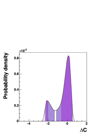
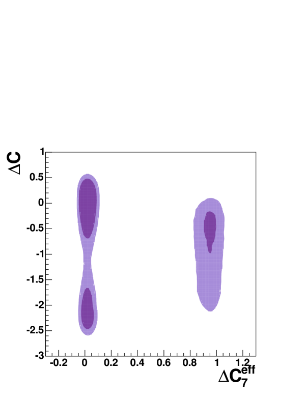
Figure 1: P.d.f.’s for $\Delta C_{7}^{\mathrm{eff}}$ (top-left), $\Delta C$ (top-right) and $\Delta C$ vs. $\Delta C_{7}^{\mathrm{eff}}$ (bottom). Dark (light) areas correspond to the $68\%$ ($95\%$) probability region.

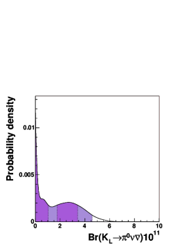
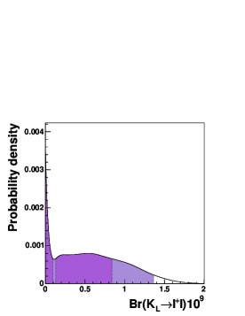
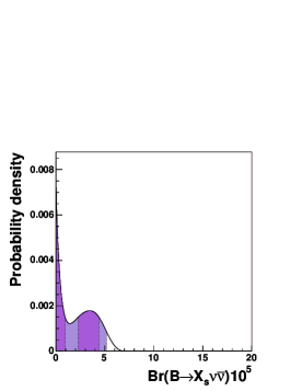
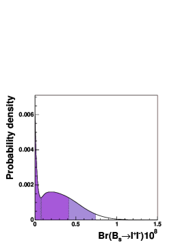
Figure 2: P.d.f.’s for the branching ratios of the rare decays $Br(K^{+}\rightarrow\pi^{+}\nu\bar{\nu})$, $Br(K_{\rm L}\rightarrow\pi^{0}\nu\bar{\nu})$, $Br(K_{\rm L}\to\mu^{+}\mu^{-})_{\rm SD}$, $Br(B\to X_{d,s}\nu\bar{\nu})$, and $Br(B_{d,s}\to\mu^{+}\mu^{-})$. Dark (light) areas correspond to the $68\%$ ($95\%$) probability region.

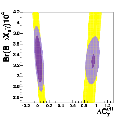
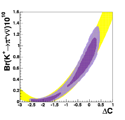
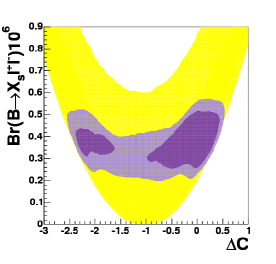
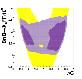
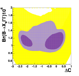
Figure 3: P.d.f.’s for the branching ratios of the rare decays used to constrain $\Delta C$ and $\Delta C_{7}^{\mathrm{eff}}$ as a function of these parameters: $Br(B\to X_{s}\gamma)_{E_{\gamma}>1.8\mathrm{GeV}}$ (top-left), $Br(K^{+}\rightarrow\pi^{+}\nu\bar{\nu})$ (top-right), $Br(B\to X_{s}l^{+}l^{-})_{14.4<q^{2}\mathrm{(GeV)}<25}$ (bottom-left), $Br(B\to X_{s}l^{+}l^{-})_{1<q^{2}\mathrm{(GeV)}<6}$ (bottom-center), $Br(B\to X_{s}l^{+}l^{-})_{0.04<q^{2}\mathrm{(GeV)}<1}$ (bottom-right). Dark (light) areas correspond to the $68\%$ ($95\%$) probability region. Very light areas correspond to the range obtained without using the experimental information.

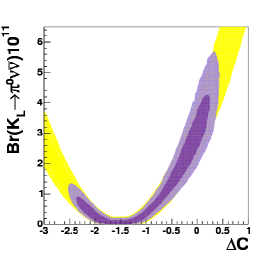
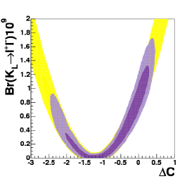
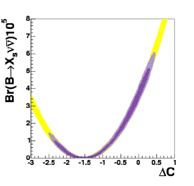
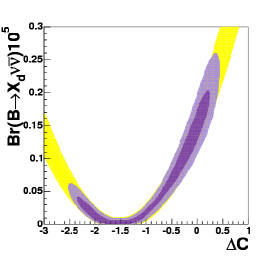
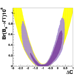
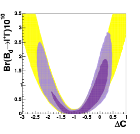
Figure 4: P.d.f.’s for the branching ratios of the rare decays $Br(K_{\rm L}\rightarrow\pi^{0}\nu\bar{\nu})$, $Br(K_{\rm L}\to\mu^{+}\mu^{-})_{\rm SD}$, $Br(B\to X_{d,s}\nu\bar{\nu})$, and $Br(B_{d,s}\to\mu^{+}\mu^{-})$ as a function of $\Delta C$. Dark (light) areas correspond to the $68\%$ ($95\%$) probability region. Very light areas correspond to the range obtained without using the experimental information.

Branching Ratios	MFV (95%)	SM (68%)	SM (95%)	exp
$Br(K^{+}\rightarrow\pi^{+}\nu\bar{\nu})\times 10^{11}$	$<11.9$	$8.3\pm 1.2$	$[6.1,10.9]$	$(14.7^{+13.0}_{-8.9})$ [19]
$Br(K_{\rm L}\rightarrow\pi^{0}\nu\bar{\nu})\times 10^{11}$	$<4.59$	$3.08\pm 0.56$	$[2.03,4.26]$	$<5.9\cdot 10^{4}$ [37]
$Br(K_{\rm L}\to\mu^{+}\mu^{-})_{\rm SD}\times 10^{9}$	$<1.36$	$0.87\pm 0.13$	$[0.63,1.15]$	-
$Br(B\to X_{s}\nu\bar{\nu})\times 10^{5}$	$<5.17$	$3.66\pm 0.21$	$[3.25,4.09]$	$<64$ [38]
$Br(B\to X_{d}\nu\bar{\nu})\times 10^{6}$	$<2.17$	$1.50\pm 0.19$	$[1.12,1.91]$	-
$Br(B_{s}\to\mu^{+}\mu^{-})\times 10^{9}$	$<7.42$	$3.67\pm 1.01$	$[1.91,5.91]$	$<2.7\cdot 10^{2}$ [39]
$Br(B_{d}\to\mu^{+}\mu^{-})\times 10^{10}$	$<2.20$	$1.04\pm 0.34$	$[0.47,1.81]$	$<1.5\cdot 10^{3}$ [39]

Table 3: Upper bounds for rare decays in MFV models at $95\%$ probability, the corresponding values in the SM (using inputs from the UUT analysis) and the available experimental information. See the text for details.

The second and third steps are carried out using the approach of ref. [40]: taking $C(v)$, $C_{7}^{\mathrm{eff}}(\mu_{b})$ and $D(v)$ to have a flat a-priori distribution and using the available experimental data and theoretical inputs, we determine the a-posteriori probability density function (p.d.f.) for $C(v)$, $C_{7}^{\mathrm{eff}}(\mu_{b})$ and all the rare decays listed in Table 3. Concerning $D(v)$, it plays only a marginal role in these decays and therefore it is not well determined by the analysis. We varied $\Delta D$ in the conservative range $\pm 4D_{\rm SM}$. Even this rather large variation has little impact on the extraction of the allowed range for $C(v)$.

In Figure 1 we plot the p.d.f. for $\Delta C(v)$ and $\Delta C_{7}^{\mathrm{eff}}$, that represent $F^{i}_{\mathrm{New}}$ in (2.1) and enter eq. (2.5). In Figure 2 we plot the p.d.f. for the branching ratios. The corresponding upper bounds at $95\%$ probability are reported in Table 3, where, for comparison, we also report the results obtained within the SM, using the same CKM parameters obtained from the UUT analysis. Finally, in Figures 3 and 4 we plot the branching ratios of the rare decays vs. $C(v)$, to make the impact of future measurements on the determination of $C(v)$ more transparent.

Let us now comment on our results. As can be seen from Figure 1, we have two possible solutions for $\Delta C_{7}^{\mathrm{eff}}$, one very close to the SM, and the other corresponding to reversing the sign of $C_{7}^{\mathrm{eff}}(\mu_{b})$ (recall that $C_{7}^{\mathrm{eff}}(\mu_{b})$ is negative in the SM and equal to $C_{7}^{\mathrm{eff}}(\mu_{b})\approx-0.33$). The second solution is disfavoured: it is barely accessible at $68\%$ probability, in accordance with the results of [14]. This result is easy to understand. In the case of the second solution for $\Delta C_{7}^{\rm eff}$, the branching ratio $Br(B\to X_{s}l^{+}l^{-})$ becomes larger than the experimental value. The full results are:

$$\Delta C_{7}^{\mathrm{eff}} = (0.02\pm 0.047)\cup(0.958\pm 0.002)\mathrm{~{}at~{}68\%~{}probability,}$$

$$\Delta C_{7}^{\mathrm{eff}} = [-0.039,0.08]\cup[0.859,1.031]\mathrm{~{}at~{}95\%~{}probability.}$$ (3.2)

Since we have two separate ranges for $\Delta C_{7}^{\mathrm{eff}}$, in the following we will also present separately the results corresponding to the “LOW” or “HI” solution for $\Delta C_{7}^{\mathrm{eff}}$ (see Figures 5 and 6).

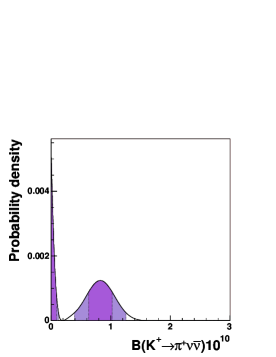
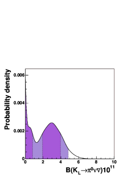
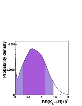
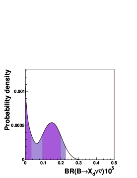
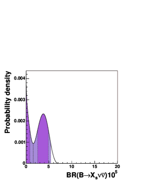
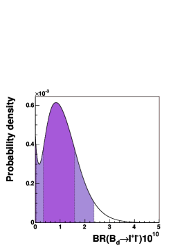
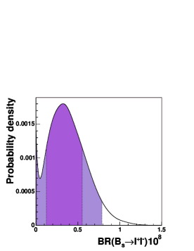
Figure 5: P.d.f.’s for the branching ratios of the rare decays $Br(K^{+}\rightarrow\pi^{+}\nu\bar{\nu})$, $Br(K_{\rm L}\rightarrow\pi^{0}\nu\bar{\nu})$, $Br(K_{\rm L}\to\mu^{+}\mu^{-})_{\rm SD}$, $Br(B\to X_{d,s}\nu\bar{\nu})$, and $Br(B_{d,s}\to\mu^{+}\mu^{-})$ considering only the LOW solution for $\Delta C_{7}^{\mathrm{eff}}$. Dark (light) areas correspond to the $68\%$ ($95\%$) probability region.

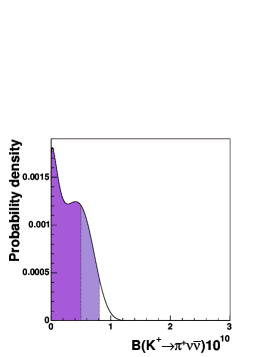
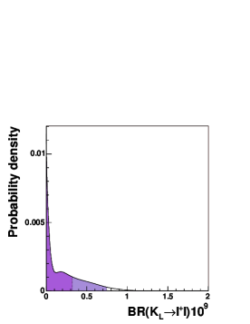
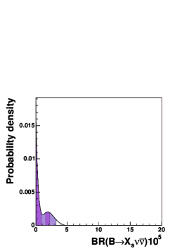
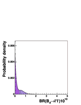
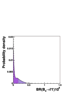
Figure 6: P.d.f.’s for the branching ratios of the rare decays $Br(K^{+}\rightarrow\pi^{+}\nu\bar{\nu})$, $Br(K_{\rm L}\rightarrow\pi^{0}\nu\bar{\nu})$, $Br(K_{\rm L}\to\mu^{+}\mu^{-})_{\rm SD}$, $Br(B\to X_{d,s}\nu\bar{\nu})$, and $Br(B_{d,s}\to\mu^{+}\mu^{-})$ considering only the HI solution for $\Delta C_{7}^{\mathrm{eff}}$. Dark (light) areas correspond to the $68\%$ ($95\%$) probability region.

As can be seen in Figure 1 we have two solutions for $\Delta C$, one close to the SM and the other corresponding to reversing the sign of $C$. We recall that $C\approx 0.81$ in the SM. The ranges obtained are

$$\Delta C = (-0.16\pm 0.53)\cup(-2.15\pm 0.08)\mathrm{~{}at~{}68\%~{}probability,}$$

$$\Delta C = [-1.25,0.44]\cup[-2.39,-1.45]\mathrm{~{}at~{}95\%~{}probability.}$$ (3.3)

From the plot of $\Delta C$ vs $\Delta C_{7}^{\mathrm{eff}}$ in Figure 1, it is evident that the situation is different for the HI and LOW solutions for $\Delta C_{7}^{\mathrm{eff}}$. Indeed, the two solutions correspond to the following ranges for $\Delta C$:

$$\mathrm{LOW:~{}}\Delta C = (-0.03\pm 0.41)\cup(-2.18\pm 0.02)\mathrm{~{}at~{}68\%~{}probability,}$$

$$\mathrm{LOW:~{}}\Delta C = [-0.75,0.50]\cup[-2.49,-1.60]\mathrm{~{}at~{}95\%~{}probability,}$$

$$\mathrm{HI:~{}}\Delta C = (-0.68\pm 0.58)\mathrm{~{}at~{}68\%~{}probability,}$$

$$\mathrm{HI:~{}}\Delta C = [-1.98,0.04]\mathrm{~{}at~{}95\%~{}probability.}$$ (3.4)

These results are easy to understand. For the LOW solution the solutions with $\Delta C$ being positive and negative are consistent with the data on $B\to X_{s}l^{+}l^{-}$. On the other hand for the HI solution, $\Delta C<0$ is favoured as with $\Delta C>0$ the difficulty with a too high $Br(B\to X_{s}l^{+}l^{-})$ becomes more acute.

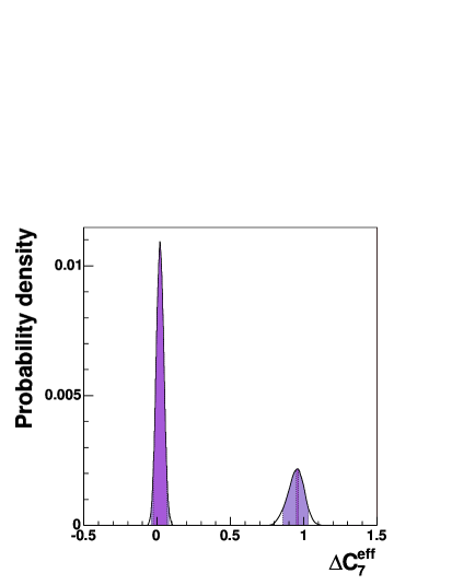
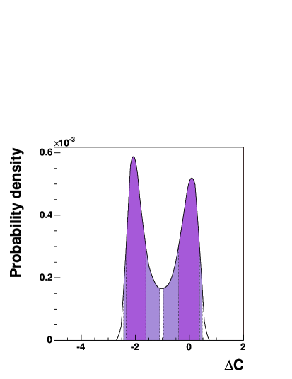
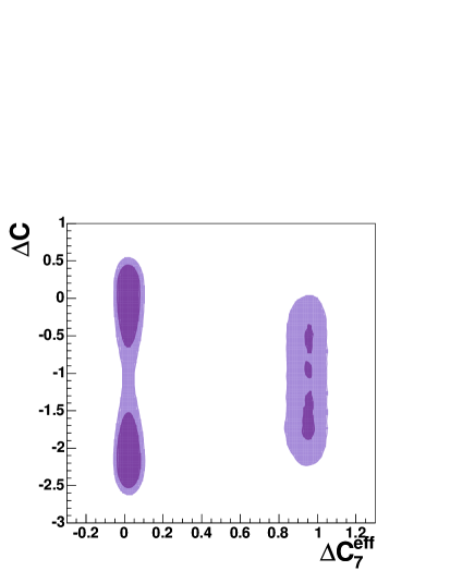
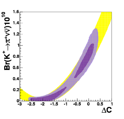
Figure 7: P.d.f.’s for $\Delta C_{7}^{\mathrm{eff}}$ (top-left), $\Delta C$ (top-right), $\Delta C$ vs. $\Delta C_{7}^{\mathrm{eff}}$ (bottom-left) and $Br(K^{+}\rightarrow\pi^{+}\nu\bar{\nu})$ vs $\Delta C$ (bottom-right) obtained without using $Br(K^{+}\rightarrow\pi^{+}\nu\bar{\nu})$ as a constraint. Dark (light) areas correspond to the $68\%$ ($95\%$) probability region.

For the reader’s convenience, we report in Table 4 the values of the $X$, $Y$ and $Z$ functions obtained by summing SM and NP contributions and by applying all the available experimental constraints.

Function	MFV (68%)	MFV (95%)
$X$	$[-0.71,-0.55]\cup[0.86,1.90]$	$[-0.86,0.10]\cup[0.30,1.95]$
$Y$	$[-1.23,-1.06]\cup[0.33,1.37]$	$[-1.38,-0.44]\cup[-0.24,1.43]$
$Z$	$[-1.51,-1.40]\cup[-0.25,1.31]$	$[-1.74,-1.05]\cup[-0.92,1.46]$

Table 4: Values at $68\%$ and $95\%$ probability for the functions $X$, $Y$ and $Z$. See the text for details.

The impact of $Br(K^{+}\rightarrow\pi^{+}\nu\bar{\nu})$ on the bounds on NP contributions can be seen by comparing Figure 1 with Figure 7, where $Br(K^{+}\rightarrow\pi^{+}\nu\bar{\nu})$ was not used as a constraint. As can be seen from Figure 7, the role of $Br(K^{+}\rightarrow\pi^{+}\nu\bar{\nu})$ is to suppress the solution with $\Delta C\sim-2$, which corresponds to destructive interference with the SM in $Br(K^{+}\rightarrow\pi^{+}\nu\bar{\nu})$ and in the other rare decays. In this respect, a further improvement of the experimental error on $Br(K^{+}\rightarrow\pi^{+}\nu\bar{\nu})$ will be extremely useful in further reducing the importance of this negative-interference solution for $\Delta C$, which is responsible for the peaks around zero for all the rare decays in Figure 2.

We also note that eliminating $\Delta C<0$ by means of $K^{+}\to\pi^{+}\nu\bar{\nu}$ would basically also eliminate the HI solution for $\Delta C_{7}^{\rm eff}$. We therefore conclude that finding $Br(K^{+}\to\pi^{+}\nu\bar{\nu})$ larger than the SM value would help in eliminating the positive sign of $C_{7}^{\rm eff}$. To our knowledge this triple correlation between $K^{+}\to\pi^{+}\nu\bar{\nu}$, $B\to X_{s}\gamma$ and $B\to X_{s}l^{+}l^{-}$ has not been discussed in the literature so far. It is very peculiar to MFV and is generally not present in models with new flavour violating contributions.

The upper bound on $Br(K^{+}\rightarrow\pi^{+}\nu\bar{\nu})$ in Table 3 has been obtained using the experimental information on this decay. It corresponds to the following $95\%$ probabilty ranges:

$$Br(K^{+}\rightarrow\pi^{+}\nu\bar{\nu}) = [0,0.17]\cup[0.24,1.19]$$ (3.5)

$$(\mathrm{LOW:~{}}[0,0.12]\cup[0.39,1.26],~{}\mathrm{HI:~{}}[0,0.81])\times 10^{-10}\,.$$

If we do not use the experimental result on $Br(K^{+}\rightarrow\pi^{+}\nu\bar{\nu})$, we obtain instead:

$$Br(K^{+}\rightarrow\pi^{+}\nu\bar{\nu}) = [0,0.15]\cup[0.28,1.12]\times 10^{-10}\,,$$ (3.6)

corresponding to an upper bound of $11.2\times 10^{-11}$ at $95\%$ probability.

We have also analyzed the decays $K_{L}\to\pi^{0}e^{+}e^{-}$ and $K_{L}\to\pi^{0}\mu^{+}\mu^{-}$ using the formulae of [29, 30]. In the models with MFV these decays are dominated by the contribution from the indirect CP violation that is basically fixed by the measured values of $\epsilon_{K}$ and $K_{S}\to\pi^{0}l^{+}l^{-}$. The dependence on $C(v)$ enters only in the subdominant direct CP-violating component and the interference of indirect and direct CP-violating contributions. We find that $Br(K_{L}\to\pi^{0}e^{+}e^{-})$ and $Br(K_{L}\to\pi^{0}\mu^{+}\mu^{-})$ can be enhanced with respect to the SM value by at most $8\%$ and $10\%$, respectively. In view of theoretical uncertainties in these decays that are larger than these enhancements, a clear signal of new physics within the MFV scenario is rather unlikely from the present perspective. Therefore we do not show the corresponding p.d.f.s.

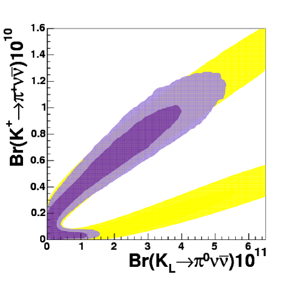
Figure 8: P.d.f. for the branching ratios of the rare decays $Br(K_{\rm L}\rightarrow\pi^{0}\nu\bar{\nu})$ vs $Br(K^{+}\rightarrow\pi^{+}\nu\bar{\nu})$. Dark (light) areas correspond to the $68\%$ ($95\%$) probability region. Very light areas correspond to the range obtained without using the experimental information.

Concerning $Br(K_{\rm L}\rightarrow\pi^{0}\nu\bar{\nu})$, its $95\%$ probability ranges are given by

$$Br(K_{\rm L}\rightarrow\pi^{0}\nu\bar{\nu}) = [0,4.59]~{}(\mathrm{LOW:~{}}[0,4.83],~{}\mathrm{HI:~{}}[0,2.84])\times 10^{-11}\,$$ (3.7)

(see Figures 2, 5 and 6). In Figure 8 we see explicitly the correlation between the charged and neutral Kaon decay modes. We observe a very strong correlation, a peculiarity of models with MFV [42]. In particular, a large enhancement of $Br(K_{\rm L}\rightarrow\pi^{0}\nu\bar{\nu})$ characteristic of models with new complex phases is not possible [43]. An observation of $Br(K_{\rm L}\rightarrow\pi^{0}\nu\bar{\nu})$ larger than $6\cdot 10^{-11}$ would be a clear signal of new complex phases or new flavour changing contributions that violate the correlations between $B$ and $K$ decays.

The $95\%$ probability ranges for $Br(K_{\rm L}\to\mu^{+}\mu^{-})_{\rm SD}$ are

$$Br(K_{\rm L}\to\mu^{+}\mu^{-})_{\rm SD} = [0,1.36]~{}(\mathrm{LOW:~{}}[0,1.44],~{}\mathrm{HI:~{}}[0,0.74])\times 10^{-9}\,.$$ (3.8)

As in the previous cases, the HI solution corresponds to a much lower upper bound.

Let us now consider $B$ decays:

$$Br(B\to X_{s}\nu\bar{\nu}) = [0,5.17]~{}(\mathrm{LOW:~{}}[0,1.56]\cup[1.59,5.4],~{}\mathrm{HI:~{}}[0,3.22])\times 10^{-5}\,,$$

$$Br(B\to X_{d}\nu\bar{\nu}) = [0,2.17]~{}(\mathrm{LOW:~{}}[0,2.26],~{}\mathrm{HI:~{}}[0,1.34])\times 10^{-6}\,,$$

$$Br(B_{s}\to\mu\bar{\mu}) = [0,7.42]~{}(\mathrm{LOW:~{}}[0,7.91],~{}\mathrm{HI:~{}}[0,3.94])\times 10^{-9}\,,$$

$$Br(B_{d}\to\mu\bar{\mu}) = [0,2.20]~{}(\mathrm{LOW:~{}}[0,2.37],~{}\mathrm{HI:~{}}[0,1.15])\times 10^{-10}\,.$$ (3.9)

The reader may wonder whether other observables could help improving the constraints on $\Delta C$ and testing MFV models. In particular, the Forward-Backward asymmetry in $B\to X_{s}l^{+}l^{-}$ is known to be a very sensitive probe of $C_{7}^{\mathrm{eff}}$ and of $C$ [44]. Indeed, the HI and LOW solutions for $\Delta C_{7}^{\mathrm{eff}}$ and corresponding possible values of $\Delta C$ give rise to different profiles of the normalized $\bar{A}_{\rm FB}$, defined as

$$\bar{A}_{\rm FB}(\hat{s})=\frac{\int_{-1}^{1}d\cos\theta_{l}\frac{d^{2}\Gamma(b\to s\mu^{+}\mu^{-})}{d\hat{s}d\cos\theta_{l}}{\rm sgn}(\cos\theta_{l})}{\int_{-1}^{1}d\cos\theta_{l}\frac{d^{2}\Gamma(b\to s\mu^{+}\mu^{-})}{d\hat{s}d\cos\theta_{l}}}\,.$$ (3.10)

This can be seen explicitly in Figure 9. Therefore, a measurement of $\bar{A}_{\rm FB}(\hat{s})$ at a Super B factory will be extremely helpful in distinguishing the various scenarios discussed above [45]. On the other hand, concerning the CP asymmetry in $B\to X_{s}\gamma$ decays [46], it turns out that in MFV models its value is reduced with respect to the SM, once the constraint on the branching ratio is taken into account, so that it is not expected to play a significant role in present and future analyses [47].

In Figure 5 we show the p.d.f.’s for the branching ratios of rare decays for the LOW solution. The corresponding result for the HI solution is given in Figure 6. Clearly the branching ratios of various decays are larger in the case of the LOW solution.

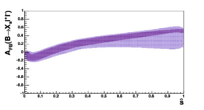
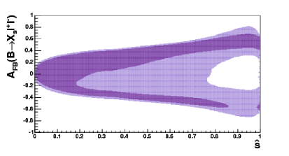
Figure 9: P.d.f.’s for the normalized forward-backward asymmetry in $B\to X_{s}l^{+}l^{-}$ for the LOW solution for $\Delta C_{7}^{\mathrm{eff}}$ with $\Delta C>-1$ (left), for the LOW solution with $\Delta C<-1$ (center) and for the HI solution for $\Delta C_{7}^{\mathrm{eff}}$ (right). Dark (light) areas correspond to the $68\%$ ($95\%$) probability region.

Before concluding this section, let us make a few steps towards the future and consider a realistic scenario for the projected integrated luminosities of Belle and BaBar, plus a $10\%$ measurement of $Br(K^{+}\rightarrow\pi^{+}\nu\bar{\nu}$). For concreteness, let us assume the following 2010 experimental data:

$$Br(B\to X_{s}l^{+}l^{-})_{0.04<q^{2}\mathrm{(GeV)}<1} = (1.13\pm 0.25)\times 10^{-6}\,,$$

$$Br(B\to X_{s}l^{+}l^{-})_{1<q^{2}\mathrm{(GeV)}<6} = \left\{\begin{array}[]{l}(1.49\pm 0.21)\times 10^{-6}\mathrm{(Belle)}\\ (1.80\pm 0.18)\times 10^{-6}\mathrm{(BaBar)}\end{array}\right.$$ (3.13)

$$Br(B\to X_{s}l^{+}l^{-})_{14.4<q^{2}\mathrm{(GeV)}<25} = \left\{\begin{array}[]{l}(4.18\pm 0.48)\times 10^{-7}\mathrm{(Belle)}\\ (5.00\pm 0.93)\times 10^{-7}\mathrm{(BaBar)}\end{array}\right.$$ (3.16)

$$Br(B\to X_{s}\gamma) = \left\{\begin{array}[]{l}(3.51\pm 0.16)\times 10^{-4}\mathrm{(Belle)}\\ (3.67\pm 0.16)\times 10^{-4}\mathrm{(BaBar~{}incl.)}\\ (3.29\pm 0.16)\times 10^{-4}\mathrm{(BaBar~{}semincl.)}\end{array}\right.$$ (3.20)

corresponding to an integrated luminosity of $1~{}{\rm ab}^{-1}$ and $700~{}{\rm fb}^{-1}$ for Belle and BaBar, respectively. Additionally a reduction to $5\%$ of the theoretical uncertainty in $Br(B\to X_{s}\gamma)$ thanks to the ongoing NNLO computation is assumed [48]. 

We can see the dramatic effect of these improvements in Figures 10-12. $B$-factory data will completely eliminate the non-standard solution for $\Delta C_{7}^{\mathrm{eff}}$, while they cannot distinguish the two solutions for $\Delta C$ (considering only branching ratio measurements), see Figure 12. However, this ambiguity is perfectly resolved by $Br(K^{+}\rightarrow\pi^{+}\nu\bar{\nu})$, leading to the impressive results in Figures 10 and 11.

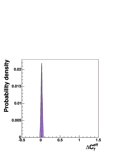
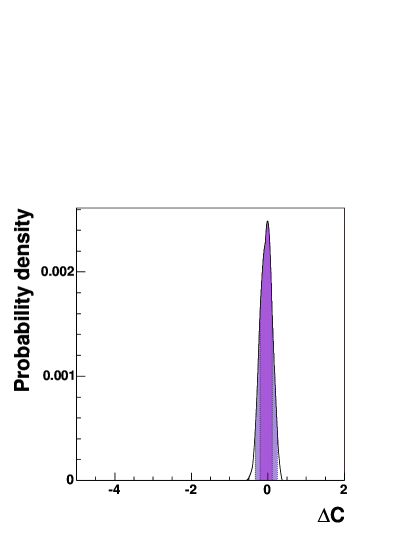
Figure 10: P.d.f.’s for $\Delta C_{7}^{\mathrm{eff}}$ (left) and $\Delta C$ (right) in the future scenario specified by eq. (3.20). Dark (light) areas correspond to the $68\%$ ($95\%$) probability region.

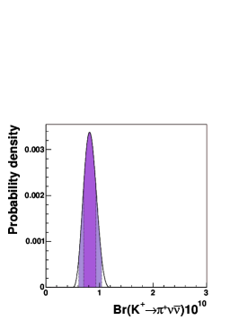
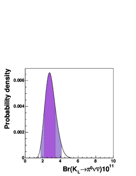
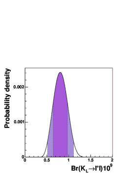
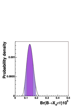
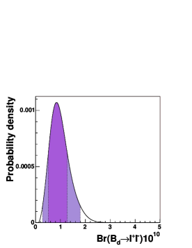
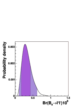
Figure 11: P.d.f.’s for the branching ratios of the rare decays $Br(K^{+}\rightarrow\pi^{+}\nu\bar{\nu})$, $Br(K_{\rm L}\rightarrow\pi^{0}\nu\bar{\nu})$, $Br(K_{\rm L}\to\mu^{+}\mu^{-})_{\rm SD}$, $Br(B\to X_{d,s}\nu\bar{\nu})$, and $Br(B_{d,s}\to\mu^{+}\mu^{-})$ in the future scenario specified by eq. (3.20). Dark (light) areas correspond to the $68\%$ ($95\%$) probability region.

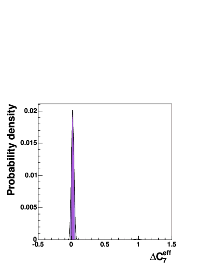
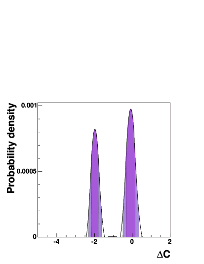
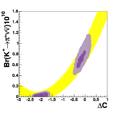
Figure 12: P.d.f.’s for $\Delta C_{7}^{\mathrm{eff}}$ (top-left), $\Delta C$ (top-right) and $Br(K^{+}\rightarrow\pi^{+}\nu\bar{\nu})$ vs $\Delta C$ (bottom) obtained without using $Br(K^{+}\rightarrow\pi^{+}\nu\bar{\nu})$ as a constraint, in the future scenario specified by eq. (3.20). Dark (light) areas correspond to the $68\%$ ($95\%$) probability region.

With so powerful experimental data, one can even think of generalizing our analysis by allowing for substantial deviations from the SM in box diagrams. If the size of new physics contributions to box diagrams is comparable to the SM ones, the results of our “future” analysis would not change sizably. On the other hand, a dramatic modification could occur for contributions to box diagrams much larger than the SM ones; however, it is very difficult to conceive new-physics models in which this possibility can be realized.

4 Messages

The main message of our paper is the following one:

The existing constraints coming from $K^{+}\to\pi^{+}\nu\bar{\nu}$, $B\to X_{s}\gamma$ and $B\to X_{s}l^{+}l^{-}$ do not allow within the MFV scenario of [5] for substantial departures of the branching ratios for all rare $K$ and $B$ decays from the SM estimates. This is evident from Table 3.

There are other messages signalled by our analysis. These are:

• The decays $B\to X_{s,d}l^{+}l^{-}$ will not offer a precise value for the function $C$ even in the presence of precise measurements of their branching ratios, unless the theoretical errors in these decays and $B\to X_{s}\gamma$ and the experimental error on the branching ratio of the latter decay are reduced substantially. This is clearly seen in Figure 3.

• The situation is considerably better in the case of $B_{d,s}\to\mu^{+}\mu^{-}$ but as seen in Figure 4, for a given value of $Br(B_{d,s}\to\mu^{+}\mu^{-})$ there are generally two solutions for $\Delta C$ and $C$, that cannot be disentangled on the basis of these decays alone.

• The great potential of the decays $K^{+}\to\pi^{+}\nu\bar{\nu}$ and $K_{L}\to\pi^{0}\nu\bar{\nu}$ in measuring the function $C$ is clearly visible in Figures 3 and 4, with the unique value obtained in the case of $K^{+}\to\pi^{+}\nu\bar{\nu}$ in the full allowed range of $C$. In the case of $K_{L}\to\pi^{0}\nu\bar{\nu}$ the two solutions are only present for $Br(K_{L}\to\pi^{0}\nu\bar{\nu})$ significant smaller that the SM value. Similar comment applies to $B\to X_{s,d}\nu\bar{\nu}$.

• Assuming that future more precise measurements of the $K\to\pi\nu\bar{\nu}$ branching ratios will be consistent with the MFV upper bounds presented here, the determination of $C$ through these decays will imply much sharper predictions for various branching ratios that could confirm or rule out the MFV scenario. In this context the correlations between various branching ratios discussed in [8] will play the crucial role.

• One of such correlations predicts that the measurement of $\sin 2\beta$ and of $Br(K^{+}\to\pi^{+}\nu\bar{\nu})$ implies only two values of $Br(K_{L}\to\pi^{0}\nu\bar{\nu})$ in the full class of MFV models that correspond to two signs of the function $X$ [42]. Figure 8 demonstrates that the solution with $X<0$, corresponding to the values in the left lower corner, is practically ruled out so that a unique prediction for $Br(K_{L}\to\pi^{0}\nu\bar{\nu})$ can in the future be obtained.

• A strong violation of any of the $95\%$ probability upper bounds on the branching ratios considered here by future measurements will imply a failure of MFV as defined in [5], unless an explicit MFV scenario can be found in which the contributions of box diagrams are significantly larger than assumed here. Dimensional arguments [43] and explicit calculations indicate that such a possibility is rather remote.

• If the only violation of the upper bounds in Table 3 occurs in $B_{s}\to\mu^{+}\mu^{-}$ and $B_{d}\to\mu^{+}\mu^{-}$, it will be most likely due to new operators beyond the SM ones. For example, the scalar operators which arise in MFV SUSY models at large $\tan\beta$ can enhance $Br(B_{s}\to\mu^{+}\mu^{-})$ up to the present experimental upper bound [9, 13, 49].

• Conversely, a violation of the upper bounds for the other channels in Table 3 would signal the presence of new sources of flavour and in particular of CP violation. This can be confirmed observing a violation of the correlations between $K$ and $B$ decays discussed above.

• In particular, recalling that in most extensions of the SM the decays $K\to\pi\nu\bar{\nu}$ are governed by the single $(V-A)\otimes(V-A)$ operator, the violation of the upper bounds on at least one of the $K\to\pi\nu\bar{\nu}$ branching ratios, will either signal the presence of new complex weak phases at work or new contributions that violate the correlations between the $B$ decays and $K$ decays.

Assuming that the MFV scenario will survive future tests, the next step will be to identify the correct model in this class. Clearly, direct searches at high energy colliders can rule out or identify specific extensions of the SM. But also FCNC processes can play an important role in this context, provided the theoretical and experimental uncertainties in some of them will be sufficiently decreased. In this case, by studying simultaneously several branching ratios it should be in principle possible to select the correct MFV models by just identifying the pattern of enhancements and suppressions relative to the SM that is specific to a given model. If this pattern is independent of the values of the parameters defining the model, no detailed quantitative analysis of the enhancements and suppressions is required in order to rule it out. As an example the distinction between the MSSM with MFV and the models with one universal extra dimension should be straightforward:

• In the MSSM with MFV the branching ratios for $K^{+}\rightarrow\pi^{+}\nu\bar{\nu}$, $K_{\rm L}\rightarrow\pi^{0}\nu\bar{\nu}$, $B\to X_{d}\nu\bar{\nu}$ and $B_{d}\to\mu^{+}\mu^{-}$ are generally suppressed relative to the SM expectations, while those governed by $V_{ts}$ like $B\to X_{s}\nu\bar{\nu}$, $B_{s}\to\mu^{+}\mu^{-}$ and $B\to X_{s}\gamma$ can be enhanced or suppressed depending on the values of parameters involved [50].

• In the model with one universal extra dimension analyzed in [22, 23], branching ratios for essentially all rare decays are enhanced, the enhancement being stronger for the decays governed by $V_{ts}$ than for those where $V_{td}$ is involved. A prominent exception is the suppression of $B\to X_{s,d}\gamma$ [23, 51].

Finally, if MFV will be confirmed, and some new particles will be observed, the rare processes discussed in this work will constitute a most powerful tool to probe the spectrum of the NP model, which might not be entirely accessible via direct studies at the LHC.

References

- [1] M. Bona et al. [UTfit Collaboration], arXiv:hep-ph/0501199.
- [2] J. Charles et al. [CKMfitter Group], arXiv:hep-ph/0406184.
- [3] M. Ciuchini, E. Franco, F. Parodi, V. Lubicz, L. Silvestrini and A. Stocchi, eConf C0304052, WG306 (2003) [arXiv:hep-ph/0307195].
- [4] M. Bona et al. [UTfit Collaboration], in preparation; Talk given by M. Pierini at the CKM 2005 Workshop, http://ckm2005.ucsd.edu/speakers/WG6/Pierini-WG6-fri2.pdf.
- [5] A. J. Buras, P. Gambino, M. Gorbahn, S. Jager and L. Silvestrini, Phys. Lett. B 500, 161 (2001) [arXiv:hep-ph/0007085].
- [6] N. Cabibbo, Phys. Rev. Lett. 10, 531 (1963).
- [7] M. Kobayashi and T. Maskawa, Prog. Theor. Phys. 49, 652 (1973).
- [8] A. J. Buras, Acta Phys. Polon. B 34, 5615 (2003) [arXiv:hep-ph/0310208].
- [9] G. D’Ambrosio, G. F. Giudice, G. Isidori and A. Strumia, Nucl. Phys. B 645, 155 (2002) [arXiv:hep-ph/0207036].
- [10] C. Bobeth, T. Ewerth, F. Krüger and J. Urban, Phys. Rev. D 66, 074021 (2002) [arXiv:hep-ph/0204225].
- [11] A. J. Buras, Phys. Lett. B 566, 115 (2003) [arXiv:hep-ph/0303060].
- [12] A. Ali, E. Lunghi, C. Greub and G. Hiller, Phys. Rev. D 66, 034002 (2002) [arXiv:hep-ph/0112300].
- [13] G. Hiller and F. Krüger, Phys. Rev. D 69, 074020 (2004) [arXiv:hep-ph/0310219].
- [14] P. Gambino, U. Haisch and M. Misiak, Phys. Rev. Lett. 94, 061803 (2005) [arXiv:hep-ph/0410155].
- [15] A. J. Buras, F. Schwab and S. Uhlig, arXiv:hep-ph/0405132.
- [16] G. Isidori, Annales Henri Poincare 4, S97 (2003) [arXiv:hep-ph/0301159]; G. Isidori, eConf C0304052, WG304 (2003) [arXiv:hep-ph/0307014].
- [17] S. C. Adler et al. [E787 Collaboration], Phys. Rev. Lett. 79, 2204 (1997) [arXiv:hep-ex/9708031]; S. C. Adler et al. [E787 Collaboration], Phys. Rev. Lett. 84, 3768 (2000) [arXiv:hep-ex/0002015].
- [18] S. Adler et al. [E787 Collaboration], Phys. Rev. Lett. 88, 041803 (2002) [arXiv:hep-ex/0111091]; S. Adler et al. [E787 Collaboration], Phys. Rev. D 70, 037102 (2004) [arXiv:hep-ex/0403034].
- [19] V. V. Anisimovsky et al. [E949 Collaboration], Phys. Rev. Lett. 93, 031801 (2004) [arXiv:hep-ex/0403036].
- [20] K. Abe et al. [Belle Collaboration], arXiv:hep-ex/0408119.
- [21] B. Aubert et al. [BABAR Collaboration], Phys. Rev. Lett. 93, 081802 (2004) [arXiv:hep-ex/0404006].
- [22] A. J. Buras, M. Spranger and A. Weiler, Nucl. Phys. B 660, 225 (2003) [arXiv:hep-ph/0212143].
- [23] A. J. Buras, A. Poschenrieder, M. Spranger and A. Weiler, Nucl. Phys. B 678, 455 (2004) [arXiv:hep-ph/0306158].
- [24] S. R. Choudhury, N. Gaur, A. Goyal and N. Mahajan, Phys. Lett. B 601, 164 (2004) [arXiv:hep-ph/0407050]; A. J. Buras, A. Poschenrieder and S. Uhlig, arXiv:hep-ph/0410309; A. J. Buras, A. Poschenrieder and S. Uhlig, arXiv:hep-ph/0501230.
- [25] G. Buchalla, A. J. Buras and M. K. Harlander, Nucl. Phys. B 349, 1 (1991).
- [26] A. J. Buras and M. K. Harlander, Adv. Ser. Direct. High Energy Phys. 10, 58 (1992).
- [27] G. Buchalla, A. J. Buras and M. E. Lautenbacher, Rev. Mod. Phys. 68, 1125 (1996) [arXiv:hep-ph/9512380].
- [28] G. Isidori, F. Mescia and C. Smith, [arXiv:hep-ph/0308008].
- [29] G. Buchalla, G. D’Ambrosio and G. Isidori, Nucl. Phys. B 672, 387 (2003) [arXiv:hep-ph/0308008].
- [30] G. Isidori, C. Smith and R. Unterdorfer, Eur. Phys. J. C 36, 57 (2004) [arXiv:hep-ph/0404127].
- [31] A. Ali and C. Greub, Z. Phys. C 49, 431 (1991); A. Ali and C. Greub, Phys. Lett. B 259, 182 (1991); A. Ali and C. Greub, Phys. Lett. B 361, 146 (1995) [arXiv:hep-ph/9506374]; A. J. Buras, A. Czarnecki, M. Misiak and J. Urban, Nucl. Phys. B 631, 219 (2002) [arXiv:hep-ph/0203135]; K. Adel and Y. P. Yao, Phys. Rev. D 49, 4945 (1994) [arXiv:hep-ph/9308349]; C. Greub and T. Hurth, Phys. Rev. D 56, 2934 (1997) [arXiv:hep-ph/9703349]; A. J. Buras, A. Kwiatkowski and N. Pott, Nucl. Phys. B 517, 353 (1998) [arXiv:hep-ph/9710336]; M. Ciuchini, G. Degrassi, P. Gambino and G. F. Giudice, Nucl. Phys. B 527, 21 (1998) [arXiv:hep-ph/9710335]; C. Bobeth, M. Misiak and J. Urban, Nucl. Phys. B 567, 153 (2000) [arXiv:hep-ph/9904413]; K. G. Chetyrkin, M. Misiak and M. Munz, Nucl. Phys. B 520, 279 (1998) [arXiv:hep-ph/9711280]; M. Misiak and M. Munz, Phys. Lett. B 344, 308 (1995) [arXiv:hep-ph/9409454]; N. Pott, Phys. Rev. D 54, 938 (1996) [arXiv:hep-ph/9512252]; Z. Ligeti, M. E. Luke, A. V. Manohar and M. B. Wise, Phys. Rev. D 60, 034019 (1999) [arXiv:hep-ph/9903305]; C. Greub, T. Hurth and D. Wyler, Phys. Lett. B 380, 385 (1996) [arXiv:hep-ph/9602281]; C. Greub, T. Hurth and D. Wyler, Phys. Rev. D 54, 3350 (1996) [arXiv:hep-ph/9603404]; A. J. Buras, A. Czarnecki, M. Misiak and J. Urban, Nucl. Phys. B 611, 488 (2001) [arXiv:hep-ph/0105160].
- [32] A. Ghinculov, T. Hurth, G. Isidori and Y. P. Yao, Nucl. Phys. B 685, 351 (2004) [arXiv:hep-ph/0312128]; C. Bobeth, P. Gambino, M. Gorbahn and U. Haisch, JHEP 0404, 071 (2004) [arXiv:hep-ph/0312090]; C. Bobeth, M. Misiak and J. Urban, Nucl. Phys. B 574, 291 (2000) [arXiv:hep-ph/9910220]; H. H. Asatryan, H. M. Asatrian, C. Greub and M. Walker, Phys. Rev. D 65, 074004 (2002) [arXiv:hep-ph/0109140]; H. H. Asatryan, H. M. Asatrian, C. Greub and M. Walker, Phys. Rev. D 66, 034009 (2002) [arXiv:hep-ph/0204341]; A. Ghinculov, T. Hurth, G. Isidori and Y. P. Yao, Nucl. Phys. B 648, 254 (2003) [arXiv:hep-ph/0208088]; H. M. Asatrian, K. Bieri, C. Greub and A. Hovhannisyan, Phys. Rev. D 66, 094013 (2002) [arXiv:hep-ph/0209006]; H. M. Asatrian, H. H. Asatryan, A. Hovhannisyan and V. Poghosyan, Mod. Phys. Lett. A 19, 603 (2004) [arXiv:hep-ph/0311187]; A. Ghinculov, T. Hurth, G. Isidori and Y. P. Yao, Eur. Phys. J. C 33, S288 (2004) [arXiv:hep-ph/0310187].
- [33] S. Chen et al. [CLEO Collaboration], Phys. Rev. Lett. 87, 251807 (2001) [arXiv:hep-ex/0108032].
- [34] P. Koppenburg et al. [Belle Collaboration], Phys. Rev. Lett. 93, 061803 (2004) [arXiv:hep-ex/0403004];
- [35] J. Walsh for the Babar Collaboration, talk presented at Moriond QCD, 2005, http://moriond.in2p3.fr/QCD/2005/SundayAfternoon/Walsh.ppt.
- [36] M. Neubert, Eur. Phys. J. C 40, 165 (2005) [arXiv:hep-ph/0408179]; D. Benson, I. I. Bigi and N. Uraltsev, Nucl. Phys. B 710, 371 (2005) [arXiv:hep-ph/0410080].
- [37] A. Alavi-Harati et al. [The E799-II/KTeV Collaboration], Phys. Rev. D 61, 072006 (2000) [arXiv:hep-ex/9907014].
- [38] R. Barate et al. [ALEPH Collaboration], Eur. Phys. J. C 19, 213 (2001) [arXiv:hep-ex/0010022].
- [39] M. Herndon[CDF and D0 Collaborations], FERMILAB-CONF-04-391-E SPIRES entry To appear in the proceedings of 32nd International Conference on High-Energy Physics (ICHEP 04), Beijing, China, 16-22 Aug 2004
- [40] M. Ciuchini et al., JHEP 0107, 013 (2001) [arXiv:hep-ph/0012308].
- [41] The experimental CL can be found at http://www.phy.bnl.gov/e949/E949Archive/br_cls.dat, and the likelihood we use can be found at http://www.utfit.org/kpinunubar/ckm-kpinunubar.html.
- [42] A. J. Buras and R. Fleischer, Phys. Rev. D 64 (2001) 115010 [arXiv:hep-ph/0104238].
- [43] A. J. Buras, A. Romanino and L. Silvestrini, Nucl. Phys. B 520, 3 (1998) [arXiv:hep-ph/9712398]; G. Colangelo and G. Isidori, JHEP 9809, 009 (1998) [arXiv:hep-ph/9808487]; A. J. Buras, G. Colangelo, G. Isidori, A. Romanino and L. Silvestrini, Nucl. Phys. B 566, 3 (2000) [arXiv:hep-ph/9908371]; G. Buchalla, G. Hiller and G. Isidori, Phys. Rev. D 63, 014015 (2001) [arXiv:hep-ph/0006136]; D. Atwood and G. Hiller, arXiv:hep-ph/0307251; A. J. Buras, R. Fleischer, S. Recksiegel and F. Schwab, Nucl. Phys. B 697, 133 (2004) [arXiv:hep-ph/0402112]; A. J. Buras, T. Ewerth, S. Jager and J. Rosiek, Nucl. Phys. B 714, 103 (2005) [arXiv:hep-ph/0408142].
- [44] G. Burdman, Phys. Rev. D 57, 4254 (1998) [arXiv:hep-ph/9710550].
- [45] A. G. Akeroyd et al.[SuperKEKB Physics Working Group], arXiv:hep-ex/0406071; J. L. Hewett et al., arXiv:hep-ph/0503261.
- [46] A. L. Kagan and M. Neubert, Phys. Rev. D 58, 094012 (1998) [arXiv:hep-ph/9803368].
- [47] T. Hurth, E. Lunghi and W. Porod, Nucl. Phys. B 704, 56 (2005) [arXiv:hep-ph/0312260].
- [48] K. Bieri, C. Greub and M. Steinhauser, Phys. Rev. D 67 (2003) 114019 [[arXiv:hep-ph/0302051]; M. Misiak and M. Steinhauser, Nucl. Phys. B 683, 277 (2004) [arXiv:hep-ph/0401041]; M. Gorbahn and U. Haisch, Nucl. Phys. B 713 (2005) 291 [arXiv:hep-ph/0411071]; M. Gorbahn, U. Haisch and M. Misiak, arXiv:hep-ph/0504194; H. M. Asatrian, C. Greub, A. Hovhannisyan, T. Hurth and V. Poghosyan, arXiv:hep-ph/0505068.
- [49] K. S. Babu and C. F. Kolda, Phys. Rev. Lett. 84, 228 (2000) [arXiv:hep-ph/9909476]; C. S. Huang, W. Liao and Q. S. Yan, Phys. Rev. D 59, 011701 (1999) [arXiv:hep-ph/9803460]; S. R. Choudhury and N. Gaur, Phys. Lett. B 451, 86 (1999) [arXiv:hep-ph/9810307]; C. S. Huang, W. Liao, Q. S. Yan and S. H. Zhu, Phys. Rev. D 63, 114021 (2001) [Erratum-ibid. D 64, 059902 (2001)] [arXiv:hep-ph/0006250]; C. Bobeth, T. Ewerth, F. Kruger and J. Urban, Phys. Rev. D 64 (2001) 074014 [arXiv:hep-ph/0104284]; A. Dedes, Mod. Phys. Lett. A 18, 2627 (2003) [arXiv:hep-ph/0309233]; A. J. Buras, P. H. Chankowski, J. Rosiek and L. Slawianowska, Phys. Lett. B 546, 96 (2002) [arXiv:hep-ph/0207241]; A. J. Buras, P. H. Chankowski, J. Rosiek and L. Slawianowska, Nucl. Phys. B 659, 3 (2003) [arXiv:hep-ph/0210145]; S. Baek, P. Ko and W. Y. Song, JHEP 0303, 054 (2003) [arXiv:hep-ph/0208112]; G. L. Kane, C. Kolda and J. E. Lennon, arXiv:hep-ph/0310042; A. Dedes and B. T. Huffman, Phys. Lett. B 600, 261 (2004) [arXiv:hep-ph/0407285].
- [50] A. J. Buras, P. Gambino, M. Gorbahn, S. Jager and L. Silvestrini, Nucl. Phys. B 592, 55 (2001) [arXiv:hep-ph/0007313].
- [51] K. Agashe, N. G. Deshpande and G. H. Wu, Phys. Lett. B 514, 309 (2001) [arXiv:hep-ph/0105084].