Abstract

This paper is a slightly modified version of the introductory part of a doctoral dissertation also containing the articles hep-ph/0303076, hep-ph/0409328 and hep-ph/0409058. The paper focuses on the calculation of particle production in a relativistic heavy ion collision using the McLerran-Venugopalan model. The main part of the paper summarizes the background of these numerical calculations. First we relate this calculation of the initial stage af a heavy ion collision to our understanding of the whole collision process. Then we discuss the saturation physics of the small $x$ wavefunction of a hadron or a nucleus. The classical field model of Kovner, McLerran and Weigert is then introduced before moving to discuss the numerical algorithms used to compute gluon and quark pair production in this model. Finally we shortly review the results on gluon and quark-antiquark production obtained in the three articles mentioned above.

Chapter 1 Introduction

Quantum Chromodynamics (QCD) has long since been firmly established as the correct theory of strong interactions; the force binding quarks into hadrons. The traditional phenomenological applications of weak coupling calculations have been in processes where there is large high (transverse) momentum scale given by one of the scattering particles, i.e. the virtual photon in deep inelastic scattering or a jet in $pp$ collisions. This hard scale ensures that the relevant value of the running coupling is small enough and higher twist corrections are suppressed. The cross section can then be factorized into universal parton distribution functions and perturbatively calculable partonic cross sections. “Bulk” observables, such as total multiplicities, have been considered so dependent on strong coupling physics that they can, even in theory, only be calculated from first principles by lattice calculations.

The Relativistic Heavy Ion Collider (RHIC) at Brookhaven (see e.g. [4, 5, 6, 7] for reviews of experimental results) has been in operation since 2000. It collides heavy ions and also lighter nuclei, deuterons and protons at different center of mass energies up to $\sqrt{s}=200A\ \textrm{GeV}$. One could estimate that the production of partons with transverse momentum of, say, $1\ \textrm{GeV}$ at central rapidities probes the nuclear wavefunction at Bjorken ${x}$ values of ${x}\sim 10^{-2}$. At the LHC, hopefully starting it operations in 2007 with $\sqrt{s}=5500A\ \textrm{GeV}$, the corresponding estimate would be ${x}\sim 2\cdot 10^{-4}$. The mean transverse momentum of produced particles, mostly pions, at RHIC is $\sim 0.5\ \textrm{GeV}$ and, as we will discuss in Sec. 2.3, it is not unreasonable to assume the mean transverse momentum of the partons produced in the initial stage of the collision to be $\sim 1-2\ \textrm{GeV}$. This means that the total multiplicity and transverse energy at RHIC and LHC are quantities that are both dominated by small ${x}$ physics and involve large enough momenta to justify using weak coupling calculations.

Because the constituents of a nucleus are Lorentz-contracted to the same transverse plane when boosted to high energy, one expects effects arising from the high density of “wee” partons to appear at higher values of ${x}$ for larger $A$. One could argue that if nonlinear effects due to the high density of partons in the proton wavefunction start to be important at ${x}\lesssim x_{0}$ (for fixed $Q^{2}$), the corresponding effects for nuclei should be seen for ${x}\lesssim Ax_{0}$. This estimate would mean that for the purpose of observing nonlinear effects due to high parton density at e.g. transverse momenta of $1\ \textrm{GeV}$ RHIC would correspond to ${x}\approx 3\cdot 10^{-5}$ and the LHC to ${x}\approx 10^{-6}$ in deep inelastic scattering on protons. Comparing to the region accessible for HERA kinematics one could also estimate that RHIC is like HERA with protons, while LHC will be more like HERA for (perhaps not very heavy) nuclei.

This new range of beam energies reached at HERA, RHIC and the LHC is so high that “bulk” phenomena might become accessible to weak coupling calculations for two reasons. Firstly, given a large enough energy density in a large enough volume (in a nuclear collision rather than, say, a $pp$ experiment) the sufficiently hard scale might be given by the temperature of the system, viewed as a blob of quark gluon plasma. Another, less universally accepted, conjecture is that at high enough energies, or equivalently small enough ${x}$, a sufficiently large momentum scale could be generated by the high density of virtual “wee” partons in the wavefunction of the accelerated hadron or nucleus and the nonlinear interactions of these partons. This latter phenomenon is referred to as saturation.

The common feature in these two concepts is that they provide a possibility to analyze “bulk” phenomena in terms of a weak coupling constant. One could say that RHIC has opened up a new “firm” region in the phenomenology of strong interactions, between the soft (hadronic and stringy) and the hard (perturbative QCD) regions. It could be characterized by the description of the system in terms of deconfined degrees of freedom, quarks and gluons, but also in terms of such high phase space densities of these partons that the nonlinearities of QCD must be treated nonperturbatively. As a digression one can mention another interesting idea prompted by the baryon excess at transverse momenta $p_{T}\sim 3-5\ \textrm{GeV}$ observed at RHIC [9, 10, 11]. This excess over both the thermal spectra at lower momenta and the one observed in dilute systems ($pp$ collions) at the same momenta has been interpreted in terms of quark recombination [12], which also relies on the large phase space density of partons.

Because saturation is inherently a high density, or strong field, phenomenon it cannot be fully understood in terms of a perturbative calculation (which is a power series in the field strength as well as the coupling constant). However, if the saturation scale $Q_{\mathrm{s}}$ (the momentum scale characterizing the density of partons at which the nonlinearities dominate) is large enough, one might still be able to perform a weak coupling calculation. The argument for a classical field approximation arises from these circumstances; one can perform nonperturbative calculations, but use the weak coupling to argue that quantum corrections can be neglected. The nonlinearities of the Yang-Mills Lagrangian (see Appendix A.2 for the explicit form) start to dominate when both terms of the covariant derivative $\partial_{\mu}+igA_{\mu}$ are of equal importance. Parametrically this means that at saturation momentum scales, $i\partial_{\mu}\sim Q_{\mathrm{s}}$, the gauge fields involved should be of order $A_{\mu}\sim Q_{\mathrm{s}}/g$. The number density of gluons $n$ should then be of order $n\sim AA\sim Q_{\mathrm{s}}^{2}/\alpha_{\mathrm{s}}$. If the transverse phase space density is high enough, $\,\mathrm{d}N/\,\mathrm{d}^{2}\mathbf{x}_{T}\sim Q_{\mathrm{s}}^{2}/\alpha_{\mathrm{s}}$ with, $Q_{\mathrm{s}}\gg\Lambda_{\mathrm{QCD}}$, then the coupling is weak and the occupation numbers of the quantum states involved $\sim 1/\alpha_{\mathrm{s}}\gg 1$. This is the region where one expects a classical approximation to be valid.

The use of the classical field approximation in QCD is also interesting becauses it involves some of the most fundamental issues in modern physics; the relation between quantum and classical theory and the wave–particle duality. The classical field approximation is also at present the most viable practical method to study time dependent phenomena in field theory.

A classical field approximation was used to study heavy ion collisions already in e.g. [13], but the idea of using the classical field approximation gained more traction with the model written down by McLerran and Venugopalan [14, 15, 16].

So far, however, most applications of saturation to phenomenology have been perturbative calculations with saturation included as some kind of phenomenological modification of perturbative gluon distributions [17, 18, 19, 20]. While this can be appropriate in some cases, such as pA-collisions at RHIC where only the nucleus is in the saturation regime [18, 21, 22, 23] or heavy quark production [24], there are phenomena like gluon production in central heavy ion collisions for which one would like to have a nonperturbative description. It is for this reason that also classical field theory computations with RHIC phenomenology in mind have been performed, starting from [25]; they are the subject of this thesis.

Now that RHIC has already been operating for several years, the best that the classical field calculations have achieved are a posteriori explanations for what has already been observed. But learning from these postdictions for RHIC we should be in a position to make more concrete quantitative predictions for the LHC results than were made before RHIC operations started [26]. For a review on applications of classical field or saturation ideas to RHIC phenomenology, see e.g. [27, 28, 29].

In the following we shall first try to convey a broad picture of a relativistic heavy ion collision in Chapter 2. In Chapter 3 we shall discuss saturation in the proton or nucleus wavefunction, how it has been studied in deep inelastic scattering and how saturation appears in the McLerran-Venugopalan model for the wavefunction. Then in Chapter 4 we turn to applying these ideas to calculating particle production in heavy ion collisions. In Chapter 5 we discuss in more detail some of the numerical methods used in these calculations. In Chapter 6 we review the results of the three publications included in this thesis [1, 2, 3] before concluding in Chapter 7.

Chapter 2 Relativistic heavy ion experiments

2.1 Spacetime picture of the collision

We shall be interested in studying the case where two nuclei move at the speed of light along the $x^{\pm}=0$-axes. These nuclei then collide and leave behind them, at finite values of $\eta$ and $\tau$, some matter which is then observed in detectors located in some region, varying between different experiments, around $\eta=0$. In order to properly interpret what is measured in the detectors one needs to understand the whole collision process.

The common baseline for understanding the spacetime evolution of the matter formed in an ultrarelativistic heavy ion collision owes much to Bjorken’s boost invariant hydrodynamical model [30] (see also [31] for a spacetime picture of the early stages of the collision). The Bjorken model assumes, based on experimental data from $p\bar{p}$-collisions, that at high enough collision energies the central rapidity region, far enough from the fragmenting nuclei, can be described as a boost invariant system, i.e. with particle phase space densities independent of spacetime rapidity $\eta.$ This model provides a relatively simple framework for understanding the collision process, but contains several assumptions that have to be theoretically understood and, if possible, experimentally verified, involving several areas physics.

1. The initial condition at $\tau=0$ depends on the properties of the nuclear wavefunction at small $x$ and the dynamics of the partonic collision process.

2. The thermal and chemical equilibration of the matter formed at $\tau\lesssim\tau_{0}$ in principle requires understanding of time dependent, nonequilibrium Quantum Field Theory.

3. The Quark Gluon Plasma phase lasts for some fermis during $\tau_{0}\lesssim\tau\lesssim\tau_{\mathrm{h}}$. For RHIC the hadronization timescale is $\tau_{\mathrm{h}}\lesssim 10\ \textrm{fm}$, for the LHC it is expected to be larger. If the system reaches local thermal equilibrium, its behavior can be described using finite temperature field theory.

4. Finally, for $\tau\gtrsim 10\ \textrm{fm}$ the system hadronizes and then after some time decouples and the particles fly to the detectors. There will be no attempt to describe in detail the setup of the detectors here, for an introduction to the detectors see e.g. [33] for RHIC and [34, 35] for the LHC.

The area of interest of this thesis are the first two phases of this picture, the initial conditions and thermalization. In Sec. 2.2 we shall discuss the more detailed experimental evidence for thermalization in heavy ion collisions and mention more fundamental studies aimed at understanding thermalization as an aspect of time dependent quantum field theory. Then in Sec. 2.3 we shall turn to what can be said about these early stages of the collision by looking at “bulk” observables, i.e. the transverse energy and multiplicity.

Apart from ion-ion collisions the nuclear wavefunction can also be independently studied in collisions between the nucleus and a more compact probe. The simplest such probe is a lepton, leading one to study deep inelastic scattering. We will discuss a saturation model approach to DIS in Sec. 3.2. Another possibility is to use a proton or, as is done at RHIC for technical reasons, a deuteron. Measurements of high $p_{T}$ particle spectra and jet-like correlations at RHIC [36, 37, 38, 39] have been essential in separating initial state nuclear or saturation effects, visible already in dAu-collisions, from effects caused by the presence of a strongly interacting medium, i.e. final state effects.

2.2 Thermalization

The matter formed in the early stages of the collision is evidently so dense and strongly interacting that it is opaque to high $p_{T}$ jets [43]. This can be inferred from the suppression of high ${\mathbf{p}_{T}}$ hadrons in central AuAu-collisions [44, 37, 36] and the disappearence of jet-like correlations between particles emitted in opposite azimuthal directions [36, 45]. But is this matter in thermal equilibrium?

The yields of different species of hadrons finally measured are remarkably well reproduced by a thermal fit [46] depending only on the decoupling temperature $T_{\mathrm{dec}}$, volume and baryochemical potential. This is an indication that the hadrons are emitted from an equilibrated system at $T=T_{\mathrm{dec}}$. It has been noticed, however, that the same kind of fit also works for $pp$ and even $e\bar{e}$-collisions [47, 48, 49] and might thus result from from a purely combinatoric argument concerning the hadronization process [50].

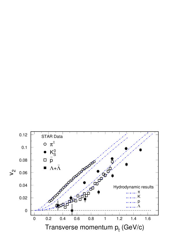
Figure 2.1: Elliptic flow $v_{2}$ of different particle species as a function of trensverse momentum. Figure and experimental data from Ref. [51], hydro calculations from Ref. [52].

Figure 2.2: Right: Transverse spectra of identified hadrons compared to hydrodynamical calculations, with $\tau_{0}=0.6\ \textrm{fm}$. The different theoretical curves are for different decoupling temperatures, $T_{\mathrm{dec}}=100\ \textrm{GeV}$ for the thick lines and $T_{\mathrm{dec}}=165\ \textrm{GeV}$ thin lines. The dashed lines have a different initial velocity profile. Figure from Ref. [53].

A perhaps more compelling argument for this scenario of thermal equilibrium and hydrodynamical evolution is the success of hydrodynamical models [54] in explaining a variety of “momentum space” experimental observables, such as elliptic flow [55] (see Fig. 2.1) and particle spectra [56, 57] (see Fig. 2.2). Hydrodynamical models have been somewhat less successful in explaining the “position space” sizes of the system as measured by HBT interferometry [58] (this is referred to as the “HBT puzzle”).

One must, of course, also be suspicious as to how much these successes of hydrodynamical is actually due to a thermal nature of the system. Although one is easily led to conclude from the experimental observations that the system indeed does thermalize early enough to justify the use of hydrodynamics, it is not yet very well understood theoretically what exacly is the timescale of thermalization and how it could happen fast enough to justify the Bjorken scenario.

There is a wide literature on thermalization in numerical calculations of real time quantum field theory [59, 60, 61, 62, 63, 64, 65] (see [66] for a recent review). These calculations, however, have so far been mostly limited to scalar field theory (although very recently also gauge theory has been studied [67]) and to 1+1 dimensions so that they are not applicable to RHIC physics. One must also point out that the geometry of the initial stages of a heavy ion collision is not a static 3 dimensional space, but rather one that is expanding in the longitudinal direction. Indeed, the phenomenologically most important aspect of thermalization is not necessarily that of the thermal (exponential) distribution of particles in different momentum modes but the isotropization of the momentum distribution between the transverse and the longitudinal degrees of freedom [68, 69].

Most perturbative estimates, e.g. the bottom-up scenario [68], generically produce quite a large thermalization time, $\tau_{0}\gtrsim 3\ \textrm{fm}$. Also approaches to chemical equilibration based on kinetic rate equations do not seem to reach chemical equilibrium fast enough to explain RHIC particle yields [70]. On the other hand, one could argue that if the behaviour of the system is characterized by some quite large momentum scale, i.e. the saturation scale $Q_{\mathrm{s}}\sim 1\ldots 2\ \textrm{GeV}$, thermalization could occur already at times $\tau_{0}\sim 1/Q_{\mathrm{s}}\sim 0.2\ \textrm{fm}$. It has been pointed out recently (see e.g. Ref. [69, 71, 72, 73, 74, 75, 76, 77]) that plasma instabilities could provide the rapid thermalization that hydrodynamical models require.

A related question is the viscosity of a strongly coupled deconfined medium. In the weak coupling limit the shear viscosity is proportional to $1/g^{4}$ . In ideal hydrodynamics the viscosity is neglected, so it would be important to know what the viscosity is in the strong coupling limit. It has been proposed that the viscosity of $N=4$ super-Yang-Mills theory in the strong coupling limit that can be calculated the AdS/CFT correspondence could give some insight into this question [80].

In this context classical field models of the nuclear wavefunction and particle production can provide some insight into understanding the collision process. Although the actual equilibrium state of a classical classical field theory is not the correct one, one could hope that the classical theory would give a reasonable phenomenological insight into the timescale of thermalization.

2.3 Transverse energy and multiplicity

The transverse energy and multiplicity at midrapidity are perhaps the most simple RHIC observables and consequently the first ones measured. They are also an example of the kind of quantity that cannot be calculated in traditional collinear perturbative QCD. Phenomenological models traditionally used to estimate this kind of quantities have been dominated by nonperturbative (“stringy”) physics (see e.g. [81]). The idea of gluon saturation at small ${x}$ opens up the fascinating possibility that such quantities could be understood with a weak coupling calculation based on the QCD Lagrangian with the nonperturbative aspects of the calculation factorized into properties of the nuclear wavefunction.

The difference between the multiplicities and energies at $\sqrt{s}=130\ \textrm{GeV}$ [82, 83, 84, 85] and $\sqrt{s}=200\ \textrm{GeV}$ [86, 87, 88, 89] is not very large at the level of accuracy of the present discussion, but let us for concreteness quote the values from Ref. [89] for the transverse energy in central collisions at $\sqrt{s}=200\ \textrm{GeV}$

$$\frac{\,\mathrm{d}E_{T}}{\,\mathrm{d}\eta}\approx 620\ \textrm{GeV}$$ (2.1)

and the ratio of the transverse energy to the charged multiplicity

$$\frac{E_{T}}{N_{\mathrm{ch}}}\approx 0.86\ \textrm{GeV}.$$ (2.2)

The particles produced in the central rapidity region are predominantly pions (to a first approximation equal numbers of $\pi^{\pm}$ and $\pi^{0}$), so we can approximate that the charged multiplicity $N_{\mathrm{ch}}$ is $2/3$ of the total multiplicity, giving

$$\frac{\,\mathrm{d}N_{\mathrm{tot}}}{\,\mathrm{d}\eta}\approx 1100.$$ (2.3)

What, then, can we infer on the properties of the system at early times from these numbers?

In the Bjorken scenario the system undergoes an isentropic boost invariant expansion staying in thermal equilibrium from the very early time until decoupling, i.e. the entropy in a unit of spacetime rapidity stays constant. The entropy is directly proportional to the number density, and thus we can directly relate the measured multiplicity to the initial state:

$$\frac{\,\mathrm{d}N^{\mathrm{init}}_{\mathrm{tot}}}{\,\mathrm{d}\eta}\approx\frac{\,\mathrm{d}N^{\mathrm{final}}_{\mathrm{tot}}}{\,\mathrm{d}\eta}\approx 1100.$$ (2.4)

In the ideal hydrodynamical Bjorken expansion the energy per unit rapidity decreases with the proper time as $\frac{\,\mathrm{d}E_{T}}{\,\mathrm{d}\eta}\sim\tau^{-1/3}$. Because the volume of the unit of spacetime rapidity is $\tau$ times the transverse area, this means that the 3-dimensional energy density $\varepsilon$ decreases like $\tau^{-4/3}$. The energy decreases because an expanding system with a pressure does $p\,\mathrm{d}V$-work, i.e. the missing energy disappears down the beampipe to larger rapidities. It is because of this phenomenon that the most important aspect of thermalization for the energy and multiplicity is the creation of a longitudinal pressure [90]. The estimate of Ref. [91], assuming an early time for starting the decrease in the transverse energy, is that the it could decrease even by a factor of $3.5$ between $\tau=0.2\ \textrm{fm}$ and decoupling. As the assumed thermalization time is very early, this could be considered an upper limit, giving an estimate for the initial state:

$$\frac{\,\mathrm{d}E_{T}(\tau=0.2\ \textrm{fm})}{\,\mathrm{d}\eta}\lesssim 2200\ \textrm{GeV}.$$ (2.5)

To express the energy density in units of $\ \textrm{GeV}/\ \textrm{fm}^{3}$ that are often used one must specify the proper time. Let us somewhat arbitrarily consider $\tau=1\ \textrm{fm}$ as a typical early time in the collision process when hydrodynamical evolution could be taken to begin. The decrease of a factor of $3.5$ in Ref. [91] assumed a very early thermalization time. If the hydrodynamical evolution is started only later at $\tau=1\ \textrm{fm}$, the transverse energy will only be able to decrease by a factor of $3.5\times(0.2\ \textrm{fm}/1\ \textrm{fm})^{1/3}\approx 2$. This leads to the estimate

$$\varepsilon(\tau=1\ \textrm{fm})=\frac{\,\mathrm{d}E_{T}(\tau=1\ \textrm{fm})}{\,\mathrm{d}\eta}\frac{1}{\tau\pi R_{A}^{2}}\lesssim 9\ \textrm{GeV}/\ \textrm{fm}^{3}.$$ (2.6)

for the 3-dimensional energy density at $\tau=1\ \textrm{fm}$. Hydrodynamical calculations with initial conditions from different saturation models have been performed in e.g. [57, 91, 92, 93, 94].

Another limit may be obtained by proceeding as in e.g. [17, 18, 20, 21, 41, 95] where, analoguously to e.g. $pp$ collisions one tries to directly relate the multiplicity of partons in the initial state to the final multiplicity without assuming thermalization or work done by a transverse pressure, simply assuming that the ratio of the parton multiplicity in the initial state and the hadron multipliciy in the final state is constant. This idea is in a sense related to the so called parton hadron duality [96]. If the system is not in thermal equilibrium, the entropy and thus the particle number density is not conserved but increases. It has also been pointed out that at least in a perturbative calculation particle number conserving collisions thermalize the partonic system quite slowly [97] and that particle number increasing processes are essential for thermalization [68], causing the multiplicity to increase.

If there is very little longitudinal $p\,\mathrm{d}V$ work done by the pressure the energy in a unit of rapidity will be conserved:

$$\frac{\,\mathrm{d}E^{\mathrm{init}}_{T}}{\,\mathrm{d}\eta}\gtrsim 600\ \textrm{GeV},$$ (2.7)

meaning that the energy density at $\tau=1\ \textrm{fm}$ would be

$$\varepsilon(\tau=1\ \textrm{fm})=\frac{\,\mathrm{d}E^{\mathrm{init}}_{T}}{\,\mathrm{d}\eta}\frac{1}{\tau\pi R_{A}^{2}}\gtrsim 4\ \textrm{GeV}/\ \textrm{fm}^{3}.$$ (2.8)

The multiplicity, on the other hand, can increase, so our estimate for the initial multiplicity, Eq. (2.4) should be taken as an upper limit:

$$\frac{\,\mathrm{d}N^{\mathrm{init}}_{\mathrm{tot}}}{\,\mathrm{d}\eta}\lesssim\frac{\,\mathrm{d}N^{\mathrm{final}}_{\mathrm{tot}}}{\,\mathrm{d}\eta}\approx 1100.$$ (2.9)

Essentially the difference between these two scenarios boils down to the difference between the energy density decreasing as $1/\tau$ for a free streaming scenario and $1/\tau^{4/3}$ for isentropic ideal hydrodynamical expansion. If the system equilibrates early and decouples late, the difference between $1/\tau$ vs. $1/\tau^{4/3}$ will be large.

We will return to these estimates and their meaning in terms of the classical field model in Chapter 6.

Chapter 3 Parton saturation in the small ${x}$ wavefunction

3.1 Parton saturation

The gluon distribution in a hadron or a nucleus, measured at a fixed virtuality $Q^{2}$, is seen in deep inelastic scattering experiments to grow towards smaller ${x}$ [98, 99]. This can be understood as resulting from a cascade of gluons radiated from the larger ${x}$ degrees of freedom into the larger phase space made available by the increasing energy $\sqrt{s}$.

The general idea of parton saturation [100, 101] is that as the transverse phase space density of gluons grows large enough, it starts to be limited by gluon fusion or, equivalently, the nonlinear interaction of the color field with itself. More specifically, the nonabelian field strength tensor consists of the linear part $\partial A$ and the nonlinear part $gA^{2}$, and for $\partial\sim{\mathbf{p}_{T}}\lesssim gA$ the nonlinearities start to dominate. In this scenario the number density of gluons would be limited from above by $n\sim AA\lesssim 1/\alpha_{\mathrm{s}}.$ The momentum scale below which this happens is called the saturation scale $Q_{\mathrm{s}}({x})$. Different authors use different conventions for the saturation scale (we shall mention some in Sec. 3.4), but to illustrate the idea let us cite one definition from [102]:

$$Q_{\mathrm{s}}^{2}(x)=\frac{8\pi^{2}\alpha_{\mathrm{s}}{N_{\mathrm{c}}}}{{N_{\mathrm{c}}}^{2}-1}\rho\sqrt{R_{A}^{2}-\mathbf{b}_{T}^{2}}xG(x,Q_{\mathrm{s}}).$$ (3.1)

This is formally an implicit equation for $Q_{\mathrm{s}}(x)$ but because the r.h.s. depends on $Q_{\mathrm{s}}(x)$ quite weakly (logarithmically) it is easy to get a reasonable approximation for the solution. In Eq. (3.1) $\rho$ is the nuclear (baryon number) density, and together with $2\sqrt{R_{A}^{2}-\mathbf{b}_{T}^{2}}$, the longitudinal extent of the nucleus at impact parameter $\mathbf{b}_{T}$, it gives a momentum scale that is inversely proportional to the transverse area of the nucleus. If one argues by the uncertainty principle that a gluon with transverse momentum $Q_{\mathrm{s}}$ has a transverse area $\sim 1/Q_{\mathrm{s}}^{2}$, Eq. (3.1) just gives an explicit definition for the saturation scale as the scale where there are on the average $\sim 1/\alpha_{\mathrm{s}}$ gluons overlapping in the nuclear wavefunction. When the strength of the interaction between these $\sim 1/\alpha_{\mathrm{s}}$ gluons is $\sim\alpha_{\mathrm{s}}$, this means that at the saturation scale (and lower momentum scales) the gluons cannot be treated as independent.

These saturation ideas have been implemented in various ways. One straighforward application in the framework of the traditional collinear factorized formulation is to approach saturation from higher momentum scales, and include the first nonlinear correction (the GLRMQ terms named after the authors of [100, 101]) in the DGLAP evolution equations. This approach has been applied e.g. to charm production [103, 104], which is an example of a quantity that is most naturally computed in the collinear factorized framework. The saturation argument has also been used to construct a successful model (the Golec-Biernat & Wusthoff model [105, 106]) for describing the HERA data for deep inelastic scattering at small ${x}$. We shall discuss this model in Sec. 3.2.

For decreasing $x$ which, for a fixed $Q^{2}$, means increasing energy, $Q_{\mathrm{s}}$ is expected to grow. For large enough energy (or for large enough nuclei) the limit $Q_{\mathrm{s}}\gg\Lambda_{\mathrm{QCD}}$ should be reached, making it possible to use weak coupling methods. Because the color fields are strong, the occupation numbers of quantum states of the system are large, and it is natural to use a classical field approximation. We shall discuss the classical field approximation in Sec. 3.3 before briefly reviewing some other points of view on parton saturation in Sec. 3.4

3.2 Saturation in DIS

Figure 3.1: In the dipole frame the incoming virtual photon splits into a quark-antiquark dipole of trensverse size $\mathbf{r}_{T}$, which then interacts with the target with the dipole cross section $\hat{\sigma}$.

It is useful to think of deep inelastic scattering at small ${x}$ in the dipole picture [107, 108, 109, 110, 111, 112], where the process is viewed as a virtual quark fluctuating into a color dipole, which then probes the wavefunction of the target (see Fig. 3.1).

In the dipole model one factorizes the total cross section into the probability for the virtual photon to fluctuate into a $q\bar{q}$ pair (a color dipole) and the cross section of the dipole scattering with the target. The total cross section can be written as [105, 112]:

$$\sigma_{\mathrm{T,L}}(x,Q^{2})=\int\,\mathrm{d}^{2}\mathbf{r}_{T}\int_{0}^{1}\,\mathrm{d}z|\psi_{\mathrm{T,L}}(z,\mathbf{r}_{T})|^{2}\hat{\sigma}(x,Q^{2},\mathbf{r}_{T}).$$ (3.2)

Here the photon wave function $\psi_{T,L}(z,\mathbf{r}_{T})$ gives the probability for the virtual photon (T and L stand for, respectively, transverse and longitudinal polarizations of the photon) to split into a color dipole of transverse size $\mathbf{r}_{T}$. The wave function $\psi_{T,L}(z,\mathbf{r}_{T})$ includes the known QED part of the reaction and is known analytically. The exact expressions can be found in e.g. Ref. [105].

It has been shown [105, 106] that the HERA data on the total [115, 116, 117, 118, 119] and the diffractive [120, 121, 122] cross sections for $x\leq 0.01$ is well reproduced by a saturation parametrization

$$\hat{\sigma}({x},Q^{2},\mathbf{r}_{T})=\sigma_{0}(1-e^{-\mathbf{r}_{T}^{2}Q_{\mathrm{s}}({x})^{2}/4}),$$ (3.3)

with the saturation scale $Q_{\mathrm{s}}^{2}$ depending on ${x}$ by

$$Q_{\mathrm{s}}^{2}({x})=({x}/x_{0})^{-\lambda}\ \textrm{GeV}^{2}.$$ (3.4)

The values found in [105] were $\sigma_{0}=23.03\ \textrm{mb},$ $x_{0}=3.04\cdot 10^{-4}$ and $\lambda=0.288$.

These fits are an example of a more general hypothesis that the behavior of the system is controlled by a universal saturation scale $Q_{\mathrm{s}}^{2}(x).$ A simple demonstration of this idea is studied in e.g. [8, 123], where a large variety of small ${x}$ deep inelastic scattering data from different experiments, with both protons and nuclei [124, 125, 126], is found to follow a universal curve when plotted as a function of the scaling variable $Q^{2}/Q_{\mathrm{s}}^{2}\sim Q^{2}{x}^{\lambda},$ instead of being functions of $Q^{2}$ and ${x}$ separately.

3.3 The classical color field of a high energy nucleus

The classical equations of motion of a nonabelian gauge field theory [127] are an interesting subject in themselves. But they are useful especially because in some circumstances the classical field approximation of the true quantum theory can be a very useful tool in understanding phenomena where high particle densities are important. One example of such a system are the soft bosonic modes of finite temperature field theory [32]. The example that concerns us in this work is the small ${x}$ wavefunction of a proton or a nucleus, where, as we argued in Sec. 3.1, the density of gluons grows large (parametrically $1/\alpha_{\mathrm{s}}$) and the high density gluonic system that is born when these quasireal gluons are freed in a relativistic heavy ion collision.

The McLerran-Venugopalan model [14, 15, 16] is a classical field model for the small ${x}$ wavefunction of a hadron or a nucleus. The correspondence between the classical field model and a diagrammatic calculation is explored in [128, 129]. Supplemented with the formulation of a collision of two ions in [130, 131] the McLerran-Venugopalan model forms the basis for what is referred to in this work as the classical field model for heavy ion collisions. We shall now concentrate on the wavefunction of one hadron or nucleus and return to colliding two of them in Chapter 4.

The central idea behind the McLerran-Venugopalan model and one that remains at the heart of the more general concept of the Color Glass Condensate is the separation between hard (large ${x}$) and small ${x}$ degrees of freedom. The former are treated as classical sources of radiation and the latter as a classical color field generated by these sources. The idea is thus to have a classical effective theory for the small ${x}$ degrees of freedom.

Let us consider a hadron or a nucleus moving at light velocity in the positive $z$ direction. The large ${x}$ degrees of freedom (the valence quarks, in a first approximation) are considered as a classical current

$$J^{\mu}=\delta^{\mu+}\delta(x^{-})\rho(\mathbf{x}_{T}).$$ (3.5)

Let us try to justify this form somewhat. The current only has a $+$-component, being caused by particles with a large $+$-component momentum. The naïve explanation for the delta function $\delta(x^{-})$ is that when the nucleus is traveling at the speed of light, it is Lorentz-contracted to an infinitesimal thickness. The more proper justification is based on the Heisenberg uncertainty principle. The large ${x}$ degrees of freedom have a large $p^{+},$ and are therefore well localized in $x^{-}$. The small ${x}$ degrees of freedom, the gluons that form the classical field, have a smaller $p^{+}$ and are spread on a larger distance in $x^{-},$ effectively seeing the sources as a delta function in $x^{-}$. The source is taken to be static in the sense that it does not depend on the light cone time $x^{+},$ because due to Lorentz time dilation the evolution in $x^{+}$ of the source is much slower than the timescales of the small ${x}$ degrees of freedom that we want to probe.

The classical color fields representing the small ${x}$ degrees of freedom are then computed using the Yang-Mills equations of motion

$$[D_{\mu},F^{\mu\nu}]=J^{\nu}.$$ (3.6)

To consistently serve as the source term of the classical equations of motion the current (3.5) must be covariantly conserved

$$[D_{\mu},J^{\mu}]=0.$$ (3.7)

In writing down Eq. (3.5) we have implicitly assumed a gauge where $A^{-}=0.$ To make the source Eq. (3.5) fully gauge invariant one would have to insert a Wilson line along the $x^{+}$-axis [132, 133] and write the source as

$$J^{\mu}=\delta^{\mu+}\delta(x^{-})W^{\dagger}(\mathbf{x}_{T},x^{+})\rho(\mathbf{x}_{T})W(\mathbf{x}_{T},x^{+}),$$ (3.8)

where the temporal Wilson line is defined as

$$W(\mathbf{x}_{T},x^{+})=P\exp\left\{ig\int_{-\infty}^{x^{+}}\,\mathrm{d}y^{+}A^{-}(\mathbf{x}_{T},y^{+})\right\}.$$ (3.9)

What yet remains unknown is the transverse color charge density $\rho(\mathbf{x}_{T})$ in the current (3.5). The argument of the original McLerran-Venugopalan model [14, 15, 16], put on a firmer group theoretical footing in [134], is the following. Let us assume that the charge density is a sum of independent color charges of a large number of hard partons. Then the resulting charge density at different points of the transverse plane should be uncorrelated. The source as a whole should be color neutral, and thus the expectation value of the charge $\langle\rho(\mathbf{x}_{T})\rangle$ should be zero. One can also argue by the central limit theorem that the distribution caused by a large number of independent charges should be Gaussian. One is thus lead to a Gaussian probablity distribution of charges

$$\langle\rho^{a}(\mathbf{x}_{T})\rho^{b}(\mathbf{y}_{T})\rangle = g^{2}\mu^{2}\delta^{2}(\mathbf{x}_{T}-\mathbf{y}_{T})\quad\textrm{ or }$$ (3.10)

$$\langle\rho^{a}({\mathbf{k}_{T}})\rho^{b}({\mathbf{p}_{T}})\rangle = (2\pi)^{2}g^{2}\mu^{2}\delta^{2}({\mathbf{k}_{T}}+{\mathbf{p}_{T}})$$ (3.11)

One could also argue [135, 136] that the charge distribution should impose color neutrality at some confinement scale $p_{T}\lesssim\Lambda_{\mathrm{QCD}}.$ In momentum space this means replacing the correlator (3.11) by

$$\langle\rho^{a}({\mathbf{k}_{T}})\rho^{b}({\mathbf{p}_{T}})\rangle=(2\pi)^{2}g^{2}\mu^{2}\delta^{2}({\mathbf{k}_{T}}+{\mathbf{p}_{T}})f({\mathbf{k}_{T}}),$$ (3.12)

where $f({\mathbf{k}_{T}})\approx 0$ for $|{\mathbf{k}_{T}}|\lesssim\Lambda_{\mathrm{QCD}}$ and $f({\mathbf{k}_{T}})\approx 1$ for $|{\mathbf{k}_{T}}|\gtrsim\Lambda_{\mathrm{QCD}}$.

One can now solve the equations of motion (3.6). The solution is most easily found in the covariant gauge $\partial_{\mu}A_{\mathrm{cov}}^{\mu}=0.$ One can find a solution with only one component of the gauge field is nonzero, namely $A_{\mathrm{cov}}^{+}(\mathbf{x}_{T},x^{-}).$ In this case Eq. (3.6) becomes a 2-dimensional Poisson equation

$$-\boldsymbol{\nabla}_{T}^{2}A_{\mathrm{cov}}^{+}=\delta(x^{-})\rho(\mathbf{x}_{T}).$$ (3.13)

We can formally write the solution as

$$A_{\mathrm{cov}}^{+}=-\delta(x^{-})\rho(\mathbf{x}_{T})/\boldsymbol{\nabla}_{T}^{2}.$$ (3.14)

Note that there is an infrared singularity in Eq. (3.14). The most natural prescription to solve this amibiguity is to impose the constraint $\int\,\mathrm{d}^{2}\mathbf{x}_{T}\rho(\mathbf{x}_{T})=0,$ i.e. to require that the source as a whole is color neutral. Imposing color neutrality at a shorter length scale will also remove this ambiguity.

The covariant gauge solution has the advantage of being localized on the light cone in the $t,z$-plane, but its interpretation in terms of partons is not very clear. To interpret the classical field in terms of quasi-real Weizsäcker-Williams gluons we must transform the field into the light cone (LC) gauge. This gauge transformation can be done using the path ordered exponential

$$U(\mathbf{x}_{T},x^{-})=\mathrm{P}\exp\left\{ig\int_{-\infty}^{x^{-}}\,\mathrm{d}y^{-}A_{\mathrm{cov}}^{+}(\mathbf{x}_{T},y^{-})\right\},$$ (3.15)

giving

$$A^{\pm}_{\mathrm{LC}} = 0$$ (3.16)

$$A^{i}_{\mathrm{LC}} = \frac{i}{g}U(\mathbf{x}_{T},x^{-})\partial_{i}U^{\dagger}(\mathbf{x}_{T},x^{-}).$$ (3.17)

The light cone gauge solution is not localized on the $x^{+}$-axis, unlike the one in covariant gauge. Instead, for $x^{-}>0$ it is a transverse pure gauge field. The field strength tensor $F^{\mu\nu},$ however, is nonzero only on the light cone $x^{-}=0$.

The problem of understanging the small ${x}$ wavefunction of the hadron or nucleus has now been reduced to a simple model depending on one phenomenological parameter describing charge density of the hard sources, $\mu$, the gauge coupling $g$, which, in the classical field approximation, is just a constant, and the geometrical properties of the hadron or nucleus. One can try to estimate the value of $\mu$ from the parton distribution functions [139] or just treat it as a parameter to be determined from experiment.

The source charge density $\mu$ increases as one probes smaller values of ${x},$ because the number of partons with higher ${x}$ than the value of interest are counted in the classical source. To study this one needs a more refined description of the longitudinal structure of the source [140]. One can then develop a renormalization group equation to see how the hard source develops as gluons of smaller and smaller ${x}$ are integrated out of the classical fields and included in the source. This renormalization group equation is the so called JIMWLK equation [132, 141, 142, 143, 144, 145, 146, 147, 148, 149, 150, 151, 152, 153].

Relation to the dipole model

In the classical field approximation the dipole cross section can be expressed in terms of Wilson lines in the background field of a nucleus [154, 155, 156, 157]

$$\hat{\sigma}(\mathbf{r}_{T})=\frac{1}{{N_{\mathrm{c}}}}\int\,\mathrm{d}^{2}\mathbf{b}_{T}\operatorname{Tr}\left\langle 1-U^{\dagger}(\mathbf{b}_{T}+\mathbf{r}_{T}/2)U(\mathbf{b}_{T}-\mathbf{r}_{T}/2)\right\rangle$$ (3.18)

where $U(\mathbf{x}_{T})$ in the Wilson line in the fundamental representation:

$$U(\mathbf{x}_{T})=\mathrm{P}\exp\left\{ig\int_{-\infty}^{\infty}\,\mathrm{d}x^{-}A_{\mathrm{cov}}^{+}(\mathbf{x}_{T},x^{-})\right\}.$$ (3.19)

The correlators of the Wilson lines in the McLerran-Venugopalan model were studied numerically in [158] and analytically in [159]. For a discussion of the different representations and conventions on the saturation scale see also [160]. Ref. [161] discusses the relation between different approaches to JIMWLK equation and how the same equation arises when considering the quantum evolution as a property of either the target wavefunction or the (dipole) probe.

By calculating the gluon distribution in the McLerran-Venugopalan model one can relate the strength of the color source to the saturation scale $Q_{\mathrm{s}}$ defined by A. Mueller and Yu. Kovchegov (see e.g. Ref. [138, 162])

$$Q_{\mathrm{s}}^{2}=\frac{g^{4}\mu^{2}C_{\mathrm{A}}}{4\pi}\ln\left(\frac{g^{4}\mu^{2}}{\Lambda_{\mathrm{QCD}}^{2}}\right).$$ (3.20)

One must also note that there is a dependence, although only a logarithmic one, on an infrared cutoff in Eq. (3.20). In analytical calculations one often argues that the relevant cutoff is $\Lambda_{\mathrm{QCD}}$, because at that scale confinement physics sets in. In numerical calculations the implicit infrared cutoff is the system size $\pi R_{A}^{2}$.

3.4 Other views of saturation

Let us then briefly mention some other views and aspects of parton saturation before proceeding to calculate gluon production in the classical field model in Chapter 4.

An interesting proposal, discussed in e.g. in Ref. [163, 164, 165, 166, 167], is to relate parton saturation to percolation. As we have noted one can argue by the Heisenberg uncertainty principle that an individual parton with transverse momentum $p_{T}$ occupies an area $\sim 1/p_{T}^{2}$ in the transverse plane. Saturation then corresponds to the situation where the wavefunctions of these partons begin to overlap and, because of their strong interactions, behave collectively. With this picture in mind one can consider saturation as a percolation phase transition. One would then expect to see clear signals of critical behavior in the system, say as a function of centrality in a heavy ion collision.

The EKRT-model [91] is a final state saturation model, where the saturation scale $p_{\mathrm{sat}}$ is determined from a geometrical saturation condition for the gluons freed in a heavy ion collision. The same scale $p_{\mathrm{sat}}$ serves as an infrared cutoff for the pQCD calculation giving the number of produced gluons in terms of usual parton distribution functions. Although the value of $p_{\mathrm{sat}}$ is close to $Q_{\mathrm{s}}$, the saturation scale in the nuclear wavefunction, it is not possible to give an explicit formula relating the two due to the different concepts of initial and final state saturation.

The saturation scale, or radius, $Q_{\mathrm{s}}=1/R_{\mathrm{s}}$ in the work of Golec-Biernat and Wusthoff [105] or Rummukainen and Weigert [151] is the same as the saturation scale $Q_{\mathrm{s}}$ of Kovchegov et. al. except with $C_{\mathrm{A}}$ replaced by $C_{\mathrm{F}}$. The technical reason for this is that they consider correlators of Wilson lines in the fundamental representation, whereas the gluon distribution that Mueller and Kovchegov consider involves the same correlator in the adjoint representation. For a comment on the relation to the saturation scale used by E. Iancu et. al., see Ref. [160].

We are using the old notation of of Krasnitz et. al. [25]. In their newer work [138] they use the parameter $\Lambda_{\mathrm{s}}$ defined as $\Lambda_{\mathrm{s}}\equiv g^{2}\mu$.

Chapter 4 Particle production in the classical field model

4.1 The classical field model

Figure 4.1: Spacetime structure of the KMcLW model. The gauge field in regions (1) and (2) are pure gauge fields on one nucleus. They are used to find the initial condition to find the gauge field in the region (3).

Let us then turn, following the approach of Kovner, McLerran and Weigert (KMcLW) [131], to studying the collision between two nuclei in the McLerran-Venugopalan model. We want to calculate the classical gauge field in the forward light cone using as initial condition the fields of the two nuclei, given by Eq. (3.16). This calculation in the light cone gauge was formulated and performed perturbatively to leading nontrivial order in [130, 131, 139] and to leading order on one of the sources and all orders in the other in [168]. The same computation can also be done in the covariant gauge [169, 170, 162].

We start with a static current of the two nuclei,

$$J^{\mu}=\delta^{\mu+}\rho_{(1)}(\mathbf{x}_{T})\delta(x^{-})+\delta^{\mu-}\rho_{(2)}(\mathbf{x}_{T})\delta(x^{+}),$$ (4.1)

anticipating the fact that we will be working in a gauge where this form is covariantly conserved. In the regions $x^{-}>0,\ x^{+}<0$ (1) and $x^{+}>0,\ x^{-}<0$ (2) (see Fig. 4.1) the field is given by the pure gauges as in Eq. (3.16)

$$A_{(m)}^{i}=\frac{i}{g}e^{i\Lambda_{(m)}}\partial_{i}e^{-i\Lambda_{(m)}},\textrm{ with }\boldsymbol{\nabla}_{T}^{2}\Lambda_{(m)}(\mathbf{x}_{T})=-g\rho_{(m)}(\mathbf{x}_{T}),\quad m=1,2.$$ (4.2)

Here we have introduced the notation $\Lambda_{(m)}$ for the solution of the Poisson equation. The quantity $\Lambda_{(m)}$ is related to to the covariant gauge fields of the nuclei by $gA^{+}_{\mathrm{cov}}=\delta(x^{-})\Lambda_{(1)},\quad gA^{-}_{\mathrm{cov}}=\delta(x^{+})\Lambda_{(2)}$.

We then choose to work in a temporal gauge $A_{\tau}=(x^{+}A^{-}+x^{-}A^{+})/\tau=0$. This will enable us to use a Hamiltonian formalism. It also matches smoothly to the conditions $A^{-}=0$ for $x^{-}=0$ and $A^{+}=0$ for $x^{+}=0$ that, as discussed in Sec. 3.3, enable us to drop the temporal Wilson lines from the current, Eq. (3.8) and use the simple form (4.1). In this gauge the remaining components of the gauge field are the transverse components $A^{i}$ and the “longitudinal” component $A_{\eta}=-\tau^{2}A^{\eta}=x^{+}A^{-}-x^{-}A^{+}$.

Inside the future light cone (region (3) in Fig. 4.1) the gauge fields satisfy the equations of motion in vacuum. What is needed is the initial condition for solving these equations. These initial conditions can be obtained by requiring that the fields in the different regions match smoothly on the light cone. In practice the initial conditions can be obtained by inserting the ansatz

$$A^{i} = \theta(-x^{+})\theta(x^{-})A^{i}_{(1)}+\theta(x^{+})\theta(-x^{-})A^{i}_{(2)}+\theta(x^{+})\theta(x^{-})A^{i}_{(3)}$$ (4.3)

$$A^{\eta} = \theta(x^{+})\theta(x^{-})A^{\eta}_{(3)}$$ (4.4)

into the equation of motion (3.6) and requiring that the singular terms arising from the derivatives of the $\theta$-functions cancel. In this way one gets the following initial conditions for the gauge field in the future light cone:

$$A^{i}_{(3)}|_{\tau=0} = A^{i}_{(1)}+A^{i}_{(2)}$$ (4.5)

$$A^{\eta}_{(3)}|_{\tau=0} = \frac{ig}{2}[A^{i}_{(1)},A^{i}_{(2)}].$$ (4.6)

The equations of motion with these initial conditions can then be solved either numerically or perturbatively in the weak field limit. Let us first look at the equations of motion in more detail and then review the weak field solution of [131] in Sec. 4.3.

4.2 Boost invariant Hamiltonian

The initial conditions, Eqs. (4.5) and (4.6), are boost invariant. Therefore it is natural to assume that also the solution of the equations of motion will be independent of rapidity. To maintain a consistent boost invariance of the solution one must not perform gauge transformations that depend on the rapidity $\eta.$ This limitation reduces the longitudinal gauge field $A_{\eta}$ to an adjoint scalar field, and we will denote it by $A_{\eta}\equiv\phi.$ We could equally well choose $A^{\eta}=-A_{\eta}/\tau^{2}$ as our canonical variable; this would simply cause powers of $\tau$ to appear in different locations (see Appendix A.1). The appearence of an adjoint scalar is analoguous to the way the time component of the gauge field becomes an adjoint scalar when dimensionally reducing high temperature gauge theory to a 3 dimensional effective theory [32]. Gauge field theory with an adjoint scalar field in the $\tau,\eta$-coordinate system has been extensively studied in [171, 172, 173, 174, 175, 176, 177].

In the gauge $A_{\tau}=0$ and with the assumption of boost invariance we end up with the following action of a 2+1-dimensional gauge theory with a scalar field in the adjoint representation,

$$S=\int\,\mathrm{d}\eta\,\mathrm{d}^{2}\mathbf{x}_{T}\,\mathrm{d}\tau\ \tau\operatorname{Tr}\bigg{\{}\dot{A_{i}}\dot{A_{i}}-\frac{1}{2}F_{ij}F_{ij}+\frac{1}{\tau^{2}}\dot{\phi}^{2}-\frac{1}{\tau^{2}}[D_{i},\phi][D_{i},\phi]\bigg{\}}.$$ (4.7)

The fields in this action are now all functions of the proper time $\tau$ and the transverse coordinate $\mathbf{x}_{T}$. A dot denotes a derivative with respect to $\tau$, i.e. $\dot{A}_{i}\equiv\partial_{\tau}A_{i}$. The explicit time dependence in the action is caused by the $\tau,\eta$-coordinate system. The expanding longitudinal geometry of the coordinate system reflects the physical situation; the collision region is expanding with light velocity as the two sources move apart from each other.

In the $A_{\tau}=0$ gauge we can go to the Hamiltonian formulation easily. Defining the canonical momenta (electric fields)

$$E^{ia} \equiv \frac{\delta S}{\delta\dot{A_{i}^{a}}}=\tau\dot{A^{a}_{i}}=-\tau\dot{A^{ai}}$$ (4.8)

$$\pi^{a} \equiv \frac{\delta S}{\delta\dot{\phi^{a}}}=\frac{1}{\tau}\dot{\phi^{a}}$$ (4.9)

we get the Hamiltonian density [172]

$$\mathcal{H} = 2\operatorname{Tr}[E^{i}\dot{A_{i}}+\pi\dot{\phi}]-\mathcal{L}$$

$$= \operatorname{Tr}\bigg{\{}\frac{1}{\tau}E^{i}E^{i}+\frac{\tau}{2}F_{ij}F_{ij}+\tau\pi^{2}+\frac{1}{\tau}[D_{i},\phi][D_{i},\phi]\bigg{\}}.$$

The first term in the Hamiltonian is the kinetic energy term of the transverse electric fields. The second term is the potential energy of the transverse gauge fields, which, in a 3-dimensional language, would be called the $z$-component of the magnetic field. In 2+1-dimensional gauge theory the magnetic field only has this one component. The third and fourth terms are the kinetic and potential energy, or electric and magnetic terms, of the scalar field.

The Hamiltonian equations of motion in the vacuum can be obtained in the standard way:

$$\dot{A}_{i} = t^{a}\frac{\delta H}{\delta E^{i}_{a}}=\frac{1}{\tau}E^{i}$$ (4.11)

$$\dot{\phi} = t^{a}\frac{\delta H}{\delta p^{a}}=\tau\pi$$ (4.12)

$$\dot{E}^{i} = -t^{a}\frac{\delta H}{\delta A_{i}^{a}}=\tau[D_{k},F_{ki}]-\frac{ig}{\tau}[\phi,[D_{i},\phi]]$$ (4.13)

$$\dot{\pi} = -t^{a}\frac{\delta H}{\delta\phi^{a}}=\frac{1}{\tau}[D_{i},[D_{i},\phi]].$$ (4.14)

Initial conditions for the Hamiltonian variables

The initial condition for the transverse gauge fields is given directly by the sum of the two transverse pure gauges, Eq. (4.5). Because the transverse electric field is proportional to $\tau$: $E^{i}=\tau\dot{A}_{i}$ its initial condition is simply $E^{i}(\tau=0,\mathbf{x}_{T})=0$. The initial condition for $A^{\eta}$ is given by the commutator of the two transverse pure gauges, Eq. (4.6). Because $\phi\equiv A_{\eta}=-\tau^{2}A^{\eta}$, this means that $\phi(\tau=0,\mathbf{x}_{T})=0$. The corresponding momentum, on the other hand, is $\pi=\dot{\phi}/\tau=-2A^{\eta}-\tau\dot{A}^{\eta}$ and thus the initial condition for $\pi$ is $\pi(\tau=0,\mathbf{x}_{T})=-ig\left[A^{i}_{(1)},A^{i}_{(2)}\right]$.

4.3 Gluon production in the weak field limit

Let us then calculate the number of gluons produced in a collision of two ultrarelativistic nuclei to the leading nontrivial order in the classical sources. Our calculation is essentially the same as performed in [131], exept that we will use the notation of the previous section. We will expand in powers of the dimensionless functions $\Lambda_{(m)}(\mathbf{x}_{T})$ defined in Eq. (4.2). They are proportional to the source strengths, $\Lambda_{(m)}(\mathbf{x}_{T})\sim g\rho_{(m)}(\mathbf{x}_{T})\sim g^{2}\mu$, so the dimensionless parameter that must be small in this computation is $g^{2}\mu/{\mathbf{k}_{T}}$. We will have to expand the fields to order $\Lambda^{2}$ and thus the multiplicity, which is quadratic in the fields, will be proportional to $\Lambda^{4}$.

Before solving the equations let us first discuss the definition of the multiplicity. Our starting point is the requirement that the energy can be expressed as an integral over momentum modes:

$$H=\int\,\mathrm{d}^{2}{\mathbf{k}_{T}}n({\mathbf{k}_{T}})|{\mathbf{k}_{T}}|.$$ (4.15)

This defines the differetial multiplicity $n({\mathbf{k}_{T}})$, assuming a massless dispersion relation $E_{\mathbf{k}_{T}}=|{\mathbf{k}_{T}}|$ and a given partition of the energy into momentum modes. We shall also take advantage of the equipartition of energy between the coordinates and the momenta in a classical mechanical system and only use only the momentum part of the Hamiltonian from Eq. (4.2),

$$H \approx 2\int\,\mathrm{d}^{2}\mathbf{x}_{T}\operatorname{Tr}\left[\frac{1}{\tau}E^{i}E^{i}+\tau\pi^{2}\right]$$

$$= 2\int\frac{\,\mathrm{d}^{2}{\mathbf{k}_{T}}}{(2\pi)^{2}}\operatorname{Tr}\left[\frac{1}{\tau}E^{i}({\mathbf{k}_{T}})E^{i}(-{\mathbf{k}_{T}})+\tau\pi({\mathbf{k}_{T}})\pi(-{\mathbf{k}_{T}})\right],$$

to define the multiplicity of gluons. The “$\approx$” should be taken as an equality in a time averaged sense. The advantage of using only the momenta is that we can easily express the kinetic part of the Hamiltonian in terms of the Fourier transforms of the momenta. Equating the expressions (4.15) and (4.3) we then find the differential multiplicity

$$n({\mathbf{k}_{T}})=\frac{1}{(2\pi)^{2}}\frac{2}{|{\mathbf{k}_{T}}|}\left[\frac{1}{\tau}E^{i}({\mathbf{k}_{T}})E^{i}(-{\mathbf{k}_{T}})+\tau\pi({\mathbf{k}_{T}})\pi(-{\mathbf{k}_{T}})\right].$$ (4.17)

Unlike the energy, the multiplicity as defined in Eq. (4.17) is not a gauge invariant concept. The prescription we shall use is to fix the Coulomb gauge in the transverse plane, $\partial_{i}A_{i}=0$.

The initial conditions for the canonical variables are, expanded to order $\Lambda^{2}$,

$$A_{i}(0,\mathbf{x}_{T}) = -\frac{1}{g}\left(\partial_{i}\Lambda_{(1)}(\mathbf{x}_{T})+\partial_{i}\Lambda_{(2)}(\mathbf{x}_{T})\right)+\frac{i}{2g}\left[\partial_{i}\Lambda_{(1)}(\mathbf{x}_{T}),\Lambda_{(1)}(\mathbf{x}_{T})\right]$$ (4.18)

$$+\frac{i}{2g}\left[\partial_{i}\Lambda_{(2)}(\mathbf{x}_{T}),\Lambda_{(2)}(\mathbf{x}_{T})\right]$$

$$\pi(0,\mathbf{x}_{T}) = \frac{i}{g}\left[\partial_{i}\Lambda_{(1)}(\mathbf{x}_{T}),\partial_{i}\Lambda_{(2)}(\mathbf{x}_{T})\right].$$ (4.19)

It is easiest to fix the Coulomb gauge already in the initial condition. This removes the lowest order terms in $A_{i}(\tau=0,\mathbf{x}_{T})$, giving

$$A_{i}^{\mathrm{Coul}}(0,\mathbf{x}_{T})=\frac{i}{2g}\left(\delta_{ij}-\frac{\partial_{i}\partial_{j}}{\boldsymbol{\nabla}_{T}^{2}}\right)\bigg{(}\left[\Lambda_{(1)}(\mathbf{x}_{T}),\partial_{j}\Lambda_{(2)}(\mathbf{x}_{T})\right]\\ +\left[\Lambda_{(2)}(\mathbf{x}_{T}),\partial_{j}\Lambda_{(1)}(\mathbf{x}_{T})\right]\bigg{)}.$$ (4.20)

From here on we will drop the superscript “Coul” and consider all fields in the Coulomb gauge for the rest of this section. Now that both $A_{i}$ and $\pi$ are of order $\Lambda^{2}$, it is easy to linearize the equations of motion Eqs. (4.11)–(4.14). They can then be solved by Fourier transforming with respect to the transverse coordinate

$$\dot{E}^{i} = \partial_{\tau}(\tau\dot{A}_{i})=\tau\boldsymbol{\nabla}_{T}^{2}A_{i}$$ (4.21)

$$\Longrightarrow \left(\tau^{2}\partial_{\tau}^{2}+\tau\partial_{\tau}+\tau^{2}{\mathbf{k}_{T}}^{2}\right)A_{i}(\tau,{\mathbf{k}_{T}})=0$$ (4.22)

$$\dot{\pi} = \partial_{\tau}\left(\frac{1}{\tau}\dot{\phi}\right)=\frac{1}{\tau}\boldsymbol{\nabla}_{T}^{2}\phi$$ (4.23)

$$\Longrightarrow \left(\tau^{2}\partial_{\tau}^{2}-\tau\partial_{\tau}+\tau^{2}{\mathbf{k}_{T}}^{2}\right)\phi(\tau,{\mathbf{k}_{T}})=0.$$ (4.24)

The solutions of these equations are Bessel functions

$$A_{i}(\tau,{\mathbf{k}_{T}}) = A_{i}(0,{\mathbf{k}_{T}})J_{0}(|{\mathbf{k}_{T}}|\tau)$$ (4.25)

$$\phi(\tau,{\mathbf{k}_{T}}) = \frac{\tau}{|{\mathbf{k}_{T}}|}\pi(0,{\mathbf{k}_{T}})J_{1}(|{\mathbf{k}_{T}}|\tau).$$ (4.26)

Using the asymptotic expansions of the Bessel functions we get the expectation value of the multiplicity

$$\langle n(\tau,{\mathbf{k}_{T}})\rangle=\frac{1}{(2\pi)^{2}}\frac{2}{\pi{\mathbf{k}_{T}}^{2}}\bigg{\{}{\mathbf{k}_{T}}^{2}\sin^{2}\left(|{\mathbf{k}_{T}}|\tau-\frac{\pi}{4}\right)\langle A_{i}^{a}(0,{\mathbf{k}_{T}})A_{i}^{a}(0,-{\mathbf{k}_{T}})\rangle\\ +\sin^{2}\left(|{\mathbf{k}_{T}}|\tau-\frac{3\pi}{4}\right)\langle\pi^{a}(0,{\mathbf{k}_{T}})\pi^{a}(0,-{\mathbf{k}_{T}})\rangle\bigg{\}}$$ (4.27)

The correlators $\langle A_{i}^{a}(0,{\mathbf{k}_{T}})A_{i}^{a}(0,-{\mathbf{k}_{T}})\rangle$ and $\langle\pi^{a}(0,{\mathbf{k}_{T}})\pi^{a}(0,-{\mathbf{k}_{T}})\rangle$ can be calculated using the initial conditions, Eqs. (4.18) and (4.19), the Poisson equation (4.2) relating the $\Lambda$’s to the charge density $\rho$ and the correlator of the charge densities, Eq. (3.10). One obtains

$$\langle A_{i}^{a}(0,{\mathbf{k}_{T}})A_{i}^{a}(0,-{\mathbf{k}_{T}})\rangle = \pi R_{A}^{2}\frac{{N_{\mathrm{c}}}({N_{\mathrm{c}}}^{2}-1)}{g^{2}}(g^{2}\mu)^{4}\int\frac{\,\mathrm{d}^{2}{\mathbf{p}_{T}}\,\mathrm{d}^{2}{\mathbf{q}_{T}}}{(2\pi)^{2}}$$

$$\delta^{2}({\mathbf{k}_{T}}-{\mathbf{p}_{T}}-{\mathbf{q}_{T}})\frac{{\mathbf{p}_{T}}^{2}{\mathbf{q}_{T}}^{2}-({\mathbf{p}_{T}}\cdot{\mathbf{q}_{T}})^{2}}{{\mathbf{k}_{T}}^{2}{\mathbf{q}_{T}}^{4}{\mathbf{p}_{T}}^{4}}$$

$$\langle\pi^{a}(0,{\mathbf{k}_{T}})\pi^{a}(0,-{\mathbf{k}_{T}})\rangle = \pi R_{A}^{2}\frac{{N_{\mathrm{c}}}({N_{\mathrm{c}}}^{2}-1)}{g^{2}}(g^{2}\mu)^{4}\int\frac{\,\mathrm{d}^{2}{\mathbf{p}_{T}}\,\mathrm{d}^{2}{\mathbf{q}_{T}}}{(2\pi)^{2}}$$

$$\delta^{2}({\mathbf{k}_{T}}-{\mathbf{p}_{T}}-{\mathbf{q}_{T}})\frac{({\mathbf{p}_{T}}\cdot{\mathbf{q}_{T}})^{2}}{{\mathbf{q}_{T}}^{4}{\mathbf{p}_{T}}^{4}}$$

Because we only used the momenta to define the multiplicity, we are left with the oscillating $\sin^{2}|{\mathbf{k}_{T}}|\tau$ factor in Eq. (4.27). We will replace this oscillating factor with its time average of $1/2$, which is equivalent to using also the contribution from the fields. To be more explicit; when we argued by the equipartition of energy and chose to use only the momenta, we effectively replaced $1=\sin^{2}|{\mathbf{k}_{T}}|\tau+\cos^{2}|{\mathbf{k}_{T}}|\tau$ by $2\sin^{2}|{\mathbf{k}_{T}}|\tau$. If we now use the time average $\overline{\sin^{2}\left(|{\mathbf{k}_{T}}|\tau\right)}=1/2$ the result will be equivalent to using both the fields and the momenta.

With this prescription the $({\mathbf{p}_{T}}\cdot{\mathbf{q}_{T}})^{2}$-terms cancel between the transverse and scalar fields and we end up with the infrared divergent result

$$\langle n({\mathbf{k}_{T}})\rangle=\frac{\pi R_{A}^{2}}{(2\pi)^{2}}\frac{{N_{\mathrm{c}}}({N_{\mathrm{c}}}^{2}-1)g^{6}\mu^{4}}{{\mathbf{k}_{T}}^{2}}\frac{1}{\pi}\int\frac{\,\mathrm{d}^{2}{\mathbf{p}_{T}}}{(2\pi)^{2}}\frac{1}{{\mathbf{p}_{T}}^{2}({\mathbf{k}_{T}}-{\mathbf{p}_{T}})^{2}}.$$ (4.30)

This is the result found in [131] (some small errors of [131] were corrected in [139], where the constant factors are correct). This result is analoguous to the bremsstrahlung result of Gunion and Bertsch [178] but with a different, in our case infrared divergent, form factor for the source (see discussion in [139]).

If we regulate the integral Eq. (4.30) with a mass $m$, replacing ${\mathbf{p}_{T}}^{2}$ and $({\mathbf{k}_{T}}-{\mathbf{p}_{T}})^{2}$ with ${\mathbf{p}_{T}}^{2}+m^{2}$ and $({\mathbf{k}_{T}}-{\mathbf{p}_{T}})^{2}+m^{2}$, it can be evaluated and we obtain

$$\langle n({\mathbf{k}_{T}})\rangle=\frac{\pi R_{A}^{2}}{(2\pi)^{3}}\frac{1}{\pi}\frac{{N_{\mathrm{c}}}({N_{\mathrm{c}}}^{2}-1)g^{6}\mu^{4}}{{\mathbf{k}_{T}}^{4}}\ln\frac{{\mathbf{k}_{T}}^{2}}{m^{2}}.$$ (4.31)

This result still has an unintegrable singularity at ${\mathbf{k}_{T}}=0$ and therefore does not give a finite result for the total multiplicity. It nevertheless has some important properties that will also hold for the full numerically computed result. The result is proportional to the transverse area of one nucleus, $\pi R_{A}^{2}$. If we assume that the infrared divergence if the integral (4.30) should be regulated at the scale $m\sim g^{2}\mu$, where, as discussed previously, our perturbative expansion breaks down, the multiplicity can be written in a general form as

$$\langle n({\mathbf{k}_{T}})\rangle=\frac{\pi R_{A}^{2}}{g^{2}}f({\mathbf{k}_{T}}/g^{2}\mu).$$ (4.32)

The numerical calculation [1] shows that when all orders in the source are included in the calculation the integrated multiplicity is indeed finite. The total multiplicity is then given in the form

$$\frac{\,\mathrm{d}N}{\,\mathrm{d}\eta}=\int\,\mathrm{d}^{2}{\mathbf{k}_{T}}\langle n({\mathbf{k}_{T}})\rangle=\frac{\pi R_{A}^{2}}{g^{2}}(g^{2}\mu)^{2}f_{N},$$ (4.33)

where

$$f_{N}\equiv\int\,\mathrm{d}^{2}\left(\frac{{\mathbf{k}_{T}}}{g^{2}\mu}\right)f\left(\frac{{\mathbf{k}_{T}}}{g^{2}\mu}\right)$$ (4.34)

is a numerical constant (i.e. independent of $g,\pi R_{A}^{2},\textrm{ and }\mu$). By the same kind of argument the transverse energy should be given by

$$\frac{\,\mathrm{d}E_{T}}{\,\mathrm{d}\eta}=\int\,\mathrm{d}^{2}{\mathbf{k}_{T}}\langle n({\mathbf{k}_{T}})\rangle|{\mathbf{k}_{T}}|=\frac{\pi R_{A}^{2}}{g^{2}}(g^{2}\mu)^{3}f_{E}.$$ (4.35)

Numerically computing the constants $f_{N}$ and $f_{E}$ is the purpose of the first article in this thesis [1]. We will discuss the numerical method for this calculation, developed in [25], in Chapter 5 and turn now to quark pair production.

4.4 Fermion pair production

Given the classical fields corresponding to gluon production a natural question to ask is: how are quark antiquark pairs produced by these color fields? Formally quark production is suppressed by $\alpha_{\textrm{s}}$ and group theory factors compared to gluons, so in a first approximation we should be able to treat the quarks as a small perturbation and neglect their backreaction on the color fields (see e.g. [179] for a comparison of quark antiquark pair and gluon production in a pQCD framework). Heavy quark production is calculable already in perturbation theory and in the weak field limit quark pair production from the classical field model reduces to a known result in $k_{\mathrm{T}}$-factorized perturbation theory [180]. It is, however, unknown how much the full inclusion of the strong color fields changes the result. Understanding light quark production would address the question of chemical equilibration; turning the color glass condensate into a quark gluon plasma. There have been calculations of quark production in heavy ion collisions from instantons [181], from static “stringy” longitudinal electric fields using the Schwinger mechanism [182, 183, 184, 185] and in the pQCD + saturation model [91, 179]. The approach of calculating the fermion Green’s functions in a space-time dependent background gauge field in Refs. [186, 187] is more similar to our approach in Ref. [3], but has not been directly applied to the gauge fields from the classical field model discussed in Sec. 4.1.

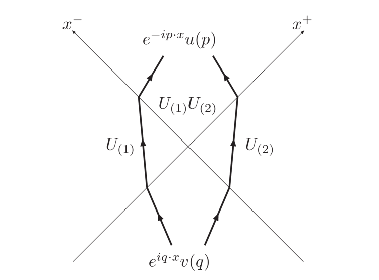
Figure 4.2: The quark antiquark pair production calculation in spacetime. We start at $x^{+}<0,\ x^{-}<0$ with a negative energy spinor on shell, $e^{iq\cdot x}v(q)$. When the antiquark line meets the first color source, it is kicked off mass shell by the color field of the source in the form of the Wilson line $U_{(1)}$ or $U_{(2)}$. When colliding with the second color source the antiquark gets another kick. The label $U_{(1)}U_{(2)}$ refers to the Abelian case, in which the field in the future light cone is a pure gauge field given by the product $U_{(1)}U_{(2)}$. In the non-Abelian case the field is known only numerically. In the end the wave function is projected to positive energy states $e^{-ip\cdot x}u(p)$ to find the pair production amplitude.

The calculation of quark pair production, outlined in more detail in Ref. [3], proceeds by solving the Dirac equation in the background color field of the two nuclei. This can be done analytically for the Abelian theory. The QED calculation, of interest for electron positron pair production in ultraperipheral collisions, is done e.g. in Ref. [188].

Let us briefly summarize the theoretical background of the calculation developed in Ref. [189]. It is well known that the cross section to produce one quark antiquark pair can be calculated by evaluating the Feynman, or time ordered, propagator for the spinor field. The time ordered propagator is also the quantity that is usually obtained when computing Feynman diagrams, because the Wick theorem applies to time ordered propagators. The main observation of Ref. [189] was that the expectation value of the number of quark antiquark pairs. is related to the retarded quark propagator. Because the Wick theorem does not apply to the retarded propagator it is difficult to calculate in perturbation theory. However, because calculating the retarded propagator is equivalent to solving the Dirac equation as an initial value problem, it is easy to formulate as a numerical calculation. One has to solve the Dirac equation with a negative energy plane wave as the initial condition. The resulting spinor is then projected to positive energy states at long enough times after the collision to obtain the quark antiquark pair multiplicity.

One can give a physical interpretation for this calculation in terms of the Dirac hole theory, where the vacuum is interpreted as a Dirac sea with all the negative energy quark states filled. Pair creation by an external field is then interpreted as the gauge field giving enough energy to a negative energy quark to lift it to a positive energy state, leaving a “hole” in the Dirac sea of negative energy quarks. This hole is then interpreted as an antiquark. The Dirac sea interpretation should of course be considered as a pedagogical explanation. The real justification for this approach is the detailed calculation in Ref. [189], where one starts by expressing the expectation value of the number of quark antiquark pairs in terms of creation and annihilation operators and then, by lengthy manipulations, relates this expression to the retarded propagator.

The initial condition for $t\to-\infty$ is a negative energy plane wave. Similarly to the QED case, one can find analytically the solution for the regions $x^{\pm}>0,\ x^{\mp}<0$, because the gauge fields in these regions are pure gauges. These then give the initial condition at $\tau=0$ for a numerical solution of the Dirac equation in the forward light cone $\tau>0$. To find the number of quark pairs one then projects the numerically calculated wave function to a positive energy plane wave at some sufficiently large time $\tau$. The structure of the calculation in different regions in spacetime is demonstrated in Fig. 4.2.

A major technical challenge in this calculation is the coordinate system. In order to include the hard sources of the color fields, the colliding nuclei, only in the initial condition of the numerical calculation, one wants to use the proper time $\tau$ instead of the Minkowski time $t$. Unlike the gluon production case, where one was able to assume strict boost invariance, one now has a nontrivial correlation between the rapidities of the quark and the antiquark. Thus, although the background gauge field is boost invariant, one must solve the Dirac equation 3+1 dimensions.

A crucial point in the calculation is the choice of the longitudinal variable to be used with $\tau$. Possible choices are $\eta,z,\textrm{ or }x^{\pm}$. To obtain the correct result we must have a dimensionful longitudinal variable, such as $z$ or $x^{\pm}$ to parametrize the $\tau=0$ surface. This is because one must be able to represent longitudinal momentum scales in coordinate space. For $\tau>0$ the corresponding longitudinal coordinate could be constructed as $\tau e^{-\eta},$ but for $\tau=0$ this is not possible. To enable a symmetric treatment of both branches in Fig. 4.2, one should choose $z$ as the longitudinal variable, with $x^{\pm}=(\sqrt{\tau^{2}+z^{2}}\pm z)/\sqrt{2}=(|z|\pm z)/\sqrt{2}$ at $\tau=0.$

One is thus led to solve numerically the Dirac equation in a curvilinear coordinate system. The covariant formulation of spinors in a curved space is a fascinating subject in itself [190], but as in this context one is merely decribing ordinary Minkowski spacetime with curved coordinates it was ultimately found in Ref. [3] that the most practical solution for this particular case is to simply change the coordinates without transforming the spinors themselves. The Dirac equation thus obtained is naturally linear in the fermion field $\psi,$ but also has an unpleasant property. Due to the choice of coordinate system and the decision to use the flat vierbein the coefficients of the time and space derivatives in the resulting Dirac equation, Eq. (5.25), depend on the coordinates. (The vierbein determines the relation between the flat tangent space where the Dirac matrices are defined to the point in spacetime. See [190] for the theory or Appendix A of Ref. [3] for a brief explanation.) As will be explained in Sec. 5.2 this makes finding a stable discretization scheme harder, and one has to use an implicit discretization scheme.

Chapter 5 Details of the numerical calculation

5.1 Classical chromodynamics on the lattice

Let us first review, following [25], how the 2+1-dimensional Hamiltonian developed in Sec. 4.2 can be cast in a form suitable for numerical simulation on a transverse lattice with a finite lattice spacing. This lattice version of the calculation has been used in many numerical studies, e.g. [1, 25, 191, 192, 193, 194, 195].

Wilson’s lattice gauge field theory was first cast in the Hamiltonian form by Kogut and Susskind [196, 197]. The classical Hamiltonian formulation has been used extensively in e.g. calculations of the sphaleron transition rate in electroweak theory [198, 199, 200, 201]. Our notations for lattice gauge theory, formulated in terms of link matrices and plaquettes, are explained in Appendix A.3.

We will start from the Wilson action (with real Minkowski time, because we want to obtain the equations of motion in real time). Then we will take the continuum limit in the $t$ and $z$-directions, leaving only the transverse coordinate discretized. This will allow us to change the coordinates to $\tau,\eta$ and restrict ourselves to $\eta$-independent field configurations. Finally we will discretize the new time coordinate $\tau$ using the leapfrog algorithm.

The Wilson action for gauge fields is

$$S=-\frac{2{N_{\mathrm{c}}}}{g^{2}}\sum_{x}\left[\sum_{1\leq i<j\leq 3}\left(1-\frac{1}{{N_{\mathrm{c}}}}\mathrm{Re}\ \operatorname{Tr}U_{i,j}(x)\right)-\sum_{i=1}^{3}\left(1-\frac{1}{{N_{\mathrm{c}}}}\mathrm{Re}\ \operatorname{Tr}U_{0,i}(x)\right)\right],$$ (5.1)

where the $-$ sign between the two terms is needed because the fields are in real, and not imaginary time. The coordinate $x$ stands for the different points in the 3+1-dimensional spacetime lattice. We then take the continuous limit in the $t$ and $z$-directions to obtain

$$S=\int\!\,\mathrm{d}z\,\mathrm{d}t\sum_{\mathbf{x}_{T}}\Bigg{[}-\frac{2{N_{\mathrm{c}}}}{g^{2}}\left(1-\frac{1}{{N_{\mathrm{c}}}}\mathrm{Re}\operatorname{Tr}U_{1,2}\right)+\frac{2}{g^{2}}\sum_{i=1}^{2}\mathrm{Re}\operatorname{Tr}[M_{0i}-M_{3i}]+\operatorname{Tr}F_{03}^{2}\Bigg{]},$$ (5.2)

where we have set the lattice spacing $a$ to unity. Here we have defined the partially continuous limit (continuous in the $\mu$-direction, $\mu=0,3$ but discrete in the $i$-direction, $i=1,2$) of the plaquette

$$M_{\mu i}(\mathbf{x}_{T})=\frac{g^{2}}{2}\left[A_{\mu}^{2}(\mathbf{x}_{T})+A_{\mu}^{2}(\mathbf{x}_{T}+\mathbf{i}_{T})\right]-igA_{\mu}(\mathbf{x}_{T})(\partial_{\mu}U_{i}(\mathbf{x}_{T}))U^{\dagger}_{i}(\mathbf{x}_{T})\\ -igA_{i}(\mathbf{x}_{T}+\mathbf{i}_{T})(\partial_{\mu}U^{\dagger}_{i}(\mathbf{x}_{T}))U_{i}(\mathbf{x}_{T})-\frac{1}{2}(\partial^{2}_{\mu}U^{\dagger}_{i}(\mathbf{x}_{T}))U_{i}(\mathbf{x}_{T})\\ -g^{2}A_{\mu}(\mathbf{x}_{T})U_{i}(\mathbf{x}_{T})A_{\mu}(\mathbf{x}_{T}+\mathbf{i}_{T})U^{\dagger}_{i}(\mathbf{x}_{T})\textrm{ (no sum over }i),$$ (5.3)

where the $t,z$ arguments have been left out for brevity and $\mathbf{i}_{T}$ denotes a unit vector in the $i$-direction, $i=1,2$.

To enable a Hamiltonian formulation we must then choose a temporal gauge condition $A_{\tau}=0.$ We shall also assume that the field configurations are boost invariant, i.e. independent of $\eta$. To consistently impose this boost invariance we must also forbid $\eta$-dependent gauge transformations, which reduces the longitudinal gauge field $A_{\eta}$ into a scalar field transforming in the adjoint representation of the gauge group. We shall consequently denote $A_{\eta}=\phi$. With these restrictions the action becomes

$$S=\int\,\mathrm{d}\eta\,\mathrm{d}\tau\sum_{\mathbf{x}_{T}}\tau\Bigg{\{}\frac{1}{g^{2}}\sum_{i}\operatorname{Tr}\left(\dot{U_{i}}^{\dagger}\dot{U_{i}}\right)-\frac{2{N_{\mathrm{c}}}}{g^{2}}\left(1-\frac{1}{{N_{\mathrm{c}}}}\mathrm{Re}\ \operatorname{Tr}U_{\bot}\right)\\ +\frac{1}{\tau^{2}}\operatorname{Tr}\dot{\phi}^{2}-\frac{1}{\tau^{2}}\sum_{i}\operatorname{Tr}\Big{(}\phi-\tilde{\phi}_{i}\Big{)}^{2}\Bigg{\}},$$ (5.4)

where $\dot{U}_{i}$ denotes the derivative with respect to $\tau$. We have also introduced the parallel transported scalar field

$$\tilde{\phi}_{i}(\mathbf{x}_{T})\equiv U_{i}(\mathbf{x}_{T})\phi(\mathbf{x}_{T}+\mathbf{i}_{T})U^{\dagger}_{i}(\mathbf{x}_{T})\textrm{ (no sum over }i).$$ (5.5)

The difference $\phi-\tilde{\phi}_{i}$ is a covariant difference, because the link matrices $U_{i}$ have been used to parallel transport $\phi(\mathbf{x}_{T}+\mathbf{i}_{T})$ so that it gauge transforms at the point $\mathbf{x}_{T}$, i.e. as

$$\tilde{\phi}_{i}(\mathbf{x}_{T})\Longrightarrow\left[V(\mathbf{x}_{T})U_{i}(\mathbf{x}_{T})V^{\dagger}(\mathbf{x}_{T}+\mathbf{i}_{T})\right]\left[V(\mathbf{x}_{T}+\mathbf{i}_{T})\phi(\mathbf{x}_{T}+\mathbf{i}_{T})V^{\dagger}(\mathbf{x}_{T}+\mathbf{i}_{T})\right]\times\\ \left[V(\mathbf{x}_{T}+\mathbf{i}_{T})U^{\dagger}_{i}(\mathbf{x}_{T})V^{\dagger}(\mathbf{x}_{T})\right]=V(\mathbf{x}_{T})\tilde{\phi}_{i}(\mathbf{x}_{T})V^{\dagger}(\mathbf{x}_{T})$$ (5.6)

and can thus be compared with $\phi(\mathbf{x}_{T})$ in a gauge invariant way.

To perform the Legendre transformation from the Lagrangian to the Hamiltonian formalism we need to replace the time derivatives in the action (5.4) by the canonical momenta, the left invariant transverse electric fields

$$E^{i}_{a}=\frac{2i\tau}{g^{2}}\operatorname{Tr}t_{a}U_{i}\dot{U_{i}}^{\dagger}\textrm{ (no sum over }i)$$ (5.7)

and the longitudinal electric fields

$$\pi=\dot{\phi}/\tau.$$ (5.8)

In terms of these canonical variables the Hamiltonian density becomes

$$\mathcal{H}=\frac{g^{2}}{\tau}\operatorname{Tr}E^{i}E^{i}+\frac{2{N_{\mathrm{c}}}\tau}{g^{2}}\left(1-\frac{1}{{N_{\mathrm{c}}}}\mathrm{Re}\operatorname{Tr}U_{1,2}\right)\\ +\tau\operatorname{Tr}\pi^{2}+\frac{1}{\tau}\sum_{i}\operatorname{Tr}\left(\phi-\tilde{\phi}_{i}\right)^{2}.$$ (5.9)

The dynamics of the theory is defined by the Hamiltonian (5.9) and the Poisson brackets between the canonical variables:

$$\{\pi^{a},\phi^{b}\} = \delta^{ab}$$ (5.10)

$$\{E_{a}^{i},U_{j}\} = it_{a}\delta^{i}_{j}U_{j}\textrm{ (no sum over }j)$$ (5.11)

$$\{E_{a}^{i},E_{b}^{j}\} = \delta^{ij}f_{abc}E_{c}^{j}\textrm{ (no sum over }j).$$ (5.12)

The first one is the usual Poisson bracket between two canonically conjugate variables. The second, Eq. (5.11) tells us that the transverse electric field $E^{i}$ generates left translations on the SU(3) group manifold of the link matrices $U_{i}$. It is actually more proper to consider the Poisson bracket Eq. (5.11) as the definition of the electric field $E^{i}$. The relation between $E^{i}$ and the time derivative of the link matrix, Eq. (5.7) then follows from this definition as the equation of motion for $U_{i}$. The third Poisson bracket, Eq. (5.12), follows directly from the second using the antisymmetry of the Poisson bracket and the Jacobi identity:

$$\{\{E_{a}^{i},E_{b}^{j}\},U_{k}\} = -\{\{E_{b}^{j},U_{k}\},E_{a}^{i}\}-\{\{U_{k},E_{a}^{i}\},E_{b}^{j}\}$$

$$= \delta^{ij}f_{abc}\{E_{c}^{j},U_{k}\}\textrm{ (no sum over }j).$$

The equations of motion for the fields can be found by taking the Poisson brackets between the fields and the Hamiltonian; the equation of motion for any quantity $v$ is $\dot{v}=\{\mathcal{H},v\}$. The equations of motion thus obtained are [1, 25]

$$\dot{U}_{i} = i\frac{g^{2}}{\tau}E^{i}U_{i}\textrm{ (no sum over }i=1,2)$$ (5.14)

$$\dot{\phi} = \tau\pi$$ (5.15)

$$\dot{E}^{1} = \frac{i\tau}{2g^{2}}\left[U_{1,2}+U_{1,-2}-\mathrm{\ h.c.\ }\right]-\textrm{trace}+\frac{i}{\tau}[\tilde{\phi}_{1},\phi]$$ (5.16)

$$\dot{E}^{2} = \frac{i\tau}{2g^{2}}\left[U_{2,1}+U_{2,-1}-\mathrm{\ h.c.\ }\right]-\textrm{trace}+\frac{i}{\tau}[\tilde{\phi}_{2},\phi]$$

$$\dot{\pi} = \frac{1}{\tau}\sum_{i}\left[\tilde{\phi}_{i}+\tilde{\phi}_{-i}-2\phi\right],$$ (5.17)

where “$-\textrm{trace}$” means that the part proportional to the identity matrix must be subtracted, because the electric fields $E^{i}$ are traceless matrices. It is easy to check that these equations are invariant under gauge transformations that depend only on the transverse coordinates. Note that although the r.h.s. of the electric field equation of motion, Eq. (5.16) depends on different plaquettes, these are all based on the same point, which makes the equation gauge invariant.

Initial conditions on the lattice

In addition to the equations of motion we also need the initial conditions corresponding to Eqs. (4.5) and (4.6) in the continuum. The initial condition for the link matrices $U_{(3)i}$ can be written as

$$\operatorname{Tr}\left[t_{a}\left[\big{(}U^{(1)}_{i}+U^{(2)}_{i}\big{)}\big{(}1+U^{{\dagger}(3)}_{i}\big{)}-\mathrm{\ h.c.\ }\right]\right]=0,$$ (5.18)

where $U_{i}^{(1,2)}$ are the pure gauge fields corresponding to the individual nuclei, given by

$$U_{i}^{(m)}(\mathbf{x}_{T})=e^{i\Lambda_{(m)}(\mathbf{x}_{T})}e^{-i\Lambda_{(m)}(\mathbf{x}_{T}+\mathbf{i}_{T})}\textrm{, with }\boldsymbol{\nabla}_{T}^{2}\Lambda_{(m)}=-g\rho_{(m)}.$$ (5.19)

By expanding the link matrices in the limit $a\to 0$ it can be verified that in the continuum limit this reduces to Eq. (4.5). Equation (5.18) is a very nonlinear equation for $U_{(3)i}$, and must be solved with some kind of iterative process. When approaching the continuum limit the link matrices are closer to the identity matrix and solving this equation numerically becomes simpler. If Eq. (5.18) is gauge transformed (with the gauge parameter depending on the transverse coordinate), the identity matrix in $1+U^{{\dagger}(3)}_{i}$ becomes a pure gauge matrix. This can be interpreted so that the identity matrix corresponds to the gauge field in the past light cone $x^{+}<0,\ x^{-}<0$. In this sense Eq. (5.18) is not gauge invariant, it applies in the specific, physically well motivated, gauge where the field vanishes in the region of spacetime where neither of the colliding nuclei has yet passed.

The initial condition for the longitudinal electric field can be written as

$$\pi(\mathbf{x}_{T})=\sum_{i}\frac{-1}{2g}\frac{i}{2}\bigg{[}\left(U_{i}^{(3)}(\mathbf{x}_{T})-1\right)\left(U_{i}^{{\dagger}(2)}(\mathbf{x}_{T})-U_{i}^{{\dagger}(1)}(\mathbf{x}_{T})\right)-\mathrm{\ h.c.\ }\\ +\left(U_{i}^{{\dagger}(3)}(\mathbf{x}_{T}-\mathbf{i}_{T})-1\right)\left(U_{i}^{(2)}(\mathbf{x}_{T}-\mathbf{i}_{T})-U_{i}^{(1)}(\mathbf{x}_{T}-\mathbf{i}_{T})\right)-\mathrm{\ h.c.\ }\bigg{]}.$$ (5.20)

It is easily verified that in the continuum limit Eq. (5.20) reduces to the corresponding commutator equation in the continuum case, Eq. (4.6). Once the more complicated initial condition for the transverse fields, Eq. (5.18), has been solved, evaluating Eq. (5.20) is a straightforward calculation.

As in the continuum case the initial conditions for the transverse electric fields and the adjoint scalar field $\phi$ are $E^{i}(\tau=0)=\phi(\tau=0)=0$.

The leapfrog algorithm

The leapfrog algorithm is commonly used in Hamiltonian time evolution of classical gauge theory. It is suited for partial differential equations that are second order in time or, equivalently, for systems where the fields (coordinates) and their time derivatives (momenta) are independent variables. The leapfrog algorithm is time reversal invariant, which guarantees second order accuracy in time. The essential idea of this algorithm is that if the coordinates are defined at times $\tau,\ \tau+\,\mathrm{d}\tau,\ \tau+2\,\mathrm{d}\tau,\dots$, the momenta are defined at timesteps $\tau+\frac{1}{2}\,\mathrm{d}\tau,\ \tau+\frac{3}{2}\,\mathrm{d}\tau,\ \tau+\frac{5}{2}\,\mathrm{d}\tau,\dots$ The momentum at $\tau+\frac{1}{2}\,\mathrm{d}\tau$ is then used to “leap” the coordinate from $\tau$ to $\tau+\,\mathrm{d}\tau$, hence the name. The only peculiarity particular about the equations of motion in this case, Eqs. (5.14)–(5.17), is the explicit time dependence, which must be treated properly in order to maintain the time reversal symmetry of the algorithm. This simply means that when stepping the fields from $\tau$ to $\tau+\,\mathrm{d}\tau$ the explicit time argument must be taken to be $\tau+\frac{1}{2}\,\mathrm{d}\tau$.

Explicitly, the timesteps can be written as

$$U_{i}(\tau+\,\mathrm{d}\tau) = \exp\left(\frac{ig^{2}\,\mathrm{d}\tau}{\tau+\,\mathrm{d}\tau/2}E^{i}(\tau+\,\mathrm{d}\tau/2)\right)U_{i}(\tau)$$ (5.21)

$$\phi(\tau+\,\mathrm{d}\tau) = \phi(\tau)+(\tau+\,\mathrm{d}\tau/2)\,\mathrm{d}\tau\pi(\tau+\,\mathrm{d}\tau/2)$$ (5.22)

$$E^{1}(\tau+\,\mathrm{d}\tau) = E^{1}(\tau)+\frac{i(\tau+\,\mathrm{d}\tau/2)\,\mathrm{d}\tau}{2g^{2}}\left.\bigg{[}U_{1,2}+U_{1,-2}-\mathrm{\ h.c.\ }-\textrm{trace}\bigg{]}\right|_{\tau+\,\mathrm{d}\tau/2}$$ (5.23)

$$+\frac{i\,\mathrm{d}\tau}{\tau+\,\mathrm{d}\tau/2}\left.\left[\tilde{\phi}_{1},\phi\right]\right|_{\tau+\,\mathrm{d}\tau/2}$$

$$E^{2}(\tau+\,\mathrm{d}\tau) = E^{2}(\tau)+\frac{i(\tau+\,\mathrm{d}\tau/2)\,\mathrm{d}\tau}{2g^{2}}\left.\bigg{[}U_{2,1}+U_{2,-1}-\mathrm{\ h.c.\ }-\textrm{trace}\bigg{]}\right|_{\tau+\,\mathrm{d}\tau/2}$$

$$+\frac{i\,\mathrm{d}\tau}{\tau+\,\mathrm{d}\tau/2}\left.\left[\tilde{\phi}_{2},\phi\right]\right|_{\tau+\,\mathrm{d}\tau/2}$$

$$\pi(\tau+\,\mathrm{d}\tau) = \pi(\tau)+\frac{\,\mathrm{d}\tau}{\tau+\,\mathrm{d}\tau/2}\sum_{i}\left.\left[\tilde{\phi}_{i}+\tilde{\phi}_{-i}-2\phi\right]\right|_{\tau+\,\mathrm{d}\tau/2},$$ (5.24)

where the parallel transported scalar field $\tilde{\phi}_{i}$ was defined in Eq. (5.5) and the index $i=1,2$ is not summed in Eq. (5.21).

5.2 Discretizing the Dirac equation in curved coordinates

Implicit discretization

Let us first discuss the general difference between an implicit and an explicit discretization [202]. Consider a partial differential equation of first order in time. Denote the values of the unknown function at a timestep $n$ by $\xi_{n},$ where $\xi_{n}$ is a vector whose components are the values of the function at different points in space, labeled by, say, $j$. The partial differential equation can be written as $\dot{\xi}=D\xi$, where $D$ is some differential operator, i.e. a matrix in position space $D_{jj^{\prime}}.$ This equation can be discretized as $\xi_{n+1}=(1+\,\mathrm{d}tD)\xi_{n}.$ This is an explicit discretization, because only the spatial derivative of the known function $\xi_{n}$ at the previous timestep is needed. If might happen that the matrix $(1+\,\mathrm{d}tD)_{jj^{\prime}}=\delta_{jj^{\prime}}+\,\mathrm{d}tD_{jj^{\prime}}$ has an eigenvalue with absolute value $>1$. In this case the discretization is unstable, even if the original equation is not. This normally gives an upper limit, the Courant-Friedrichs-Lewy (CFL) condition, for the size of the timestep $\,\mathrm{d}t$. An example of an implicit discretization, on the other hand, would be $(1-\,\mathrm{d}tD)\xi_{n+1}=\xi_{n},$ requiring one to solve a system of equations (a linear one if $D$ is independent of the $\xi$) to find $\xi_{n+1}$ at each timestep. The two discretization schemes are formally equally accurate (to first order in $\,\mathrm{d}t$), but the implicit one is usually stable for reasonable differential operators $D.$

We shall now proceed to discretizing the Dirac equation in $\tau,z$-coordinates implicitly and showing in detail how the resulting linear system can be solved using LU-decomposition [202]. Let us note, in passing, that it might well turn out that to solve the 3+1-dimensional Yang-Mills equations in a coordinate system where the time variable is $\tau,$ one will probably also have to use an implicit discretization also. This is more difficult than the present case, because unlike the Dirac equation, the equations are not linear. Nevertheless, an implicit scheme has already been used in Yang-Mills theory [203], so the task should not be impossible.

Dirac equation in $\tau,z$-coordinates

It is useful to separate the Dirac spinor $\psi$ into eigenvectors of $\gamma^{0}\gamma^{3}$, by the projection operators $P^{\pm}=\frac{1}{2}(1\pm\gamma^{0}\gamma^{3})$. In the $\tau,z$-coordinate system and for these components separately the Dirac equation with an external gauge field is:

$$\partial_{\tau}\psi^{\pm}=\frac{\sqrt{\tau^{2}+z^{2}}\pm z}{\tau}\left(\mp\partial_{z}\psi^{\pm}+i\gamma^{0}(i{\boldsymbol{\gamma}_{T}}\cdot{\mathbf{D}_{T}}-m)\psi^{\mp}\right)\mp i\frac{\phi}{\tau}\psi^{\pm}.$$ (5.25)

Here we are using the same gauge as in the numerical calculation of gluon production, namely $A_{\tau}=0$. We also assume that the background gauge field is independent of rapidity and thus the longitudinal gauge field is an adjoint scalar field. From now on we absorb the coupling constant into the field and denote $\phi\equiv gA_{\eta}$. To shorten the notation we shall also denote the timestep with a subscript $n$ and the lattice site in the longitudinal $z$-direction with a superscript $j$. We discretize the Dirac equation implicitly as

$$\frac{1}{2\,\mathrm{d}\tau}\left(P^{\pm}\psi^{j}_{n+1}-P^{\pm}\psi^{j}_{n-1}\right)\\ =\mp\frac{\sqrt{\tau^{2}+z^{2}}\pm z}{4\,\mathrm{d}z\tau}\left[P^{\pm}\psi^{j+1}_{n+1}+P^{\pm}\psi^{j+1}_{n-1}-P^{\pm}\psi^{j-1}_{n+1}-P^{\pm}\psi^{j-1}_{n-1}\right]\\ +i\frac{\sqrt{\tau^{2}+z^{2}}\pm z}{\tau}\gamma^{0}(i{\boldsymbol{\gamma}_{T}}\cdot{\mathbf{D}_{T}}-m)P^{\mp}\psi^{j}_{n}\mp i\frac{\phi_{n}}{2\tau}P^{\pm}\left[\psi^{j}_{n+1}+\psi^{j}_{n-1}\right]$$ (5.26)

Multiplying by $2\,\mathrm{d}\tau$ and solving we get

$$\left(1\pm i\frac{\phi_{n}\,\mathrm{d}\tau}{\tau}\right)P^{\pm}\psi^{j}_{n+1}\pm\frac{\sqrt{\tau^{2}+z^{2}}\pm z}{2\,\mathrm{d}z\tau}\,\mathrm{d}\tau\left[P^{\pm}\psi^{j+1}_{n+1}-P^{\pm}\psi^{j-1}_{n+1}\right]\\ =\left(1\mp i\frac{\phi_{n}\,\mathrm{d}\tau}{\tau}\right)P^{\pm}\psi^{j}_{n-1}\mp\frac{\sqrt{\tau^{2}+z^{2}}\pm z}{2\,\mathrm{d}z\tau}\,\mathrm{d}\tau\left[P^{\pm}\psi^{j+1}_{n-1}-P^{\pm}\psi^{j-1}_{n-1}\right]\\ -\frac{\sqrt{\tau^{2}+z^{2}}\pm z}{\tau}2\,\mathrm{d}\tau\gamma^{0}({\boldsymbol{\gamma}_{T}}\cdot{\mathbf{D}_{T}}+im)P^{\mp}\psi^{j}_{n}\equiv\xi^{j}_{n}.$$ (5.27)

Now we must address the question of the boundaries in the $z$-direction. Periodic boundary conditions can be used in the transverse direction, but not for the longitudinal coordinate, because the equation is not invariant under translations in the $z$-direction at fixed proper time $\tau$. We choose free boundary conditions, not setting any restriction on $\psi$ at the boundary. In practice this means the following. Let us denote the endpoints of the lattice by $j=\pm J$, i.e. the longitudinal lattice consists of $2J+1$ points. When for the points in the interior of the lattice the longitudinal derivative was discretized using the difference $\psi^{j+1}-\psi^{j-1}\approx 2\,\mathrm{d}z(\partial_{z}\psi)^{j}$, for the endpoints this must be replaced by $3\psi^{J}+\psi^{J-2}-4\psi^{J-1}\approx 2\,\mathrm{d}z(\partial_{z}\psi)^{J}$ and $4\psi^{-J+1}-3\psi^{-J}-\psi^{-J+2}\approx 2\,\mathrm{d}z(\partial_{z}\psi)^{-J}$.

Equation (5.27) gives us a system of linear equations to solve at each timestep. The coefficients of the system are $3\times 3$ complex matrices because of the gauge fields in the equation. Note that although we need the spinor at both timesteps $n-1$ and $n$ to find $\psi_{n+1}$, the $P^{\pm}$ components decouple in such a way that we only need to store the values of $\psi$ at one timestep, i.e. after using $P^{+}\psi_{n-1}$ and $P^{-}\psi_{n}$ to find $P^{+}\psi_{n+1}$ we can then forget $P^{+}\psi_{n-1}$ and move to the next timestep to solve for $P^{-}\psi_{n+2}$. The linear system Eq. (5.27) is most efficiently solved by LU-decomposition in a way that we will review next.

Solving the tridiagonal system by LU-decomposition

Let us write the linear system, Eq. (5.27), as

$$MP^{\pm}\psi_{n+1}=\xi_{n},$$ (5.28)

where $\xi_{n}$ as defined by the r.h.s. of Eq. (5.27) is known and $P^{\pm}\psi_{n+1}$ is unknown. The coefficients of the matrix $M$ can be read off Eq. (5.27) taking into account the special treatment of the boundary in the $z$-direction. The matrix $M$ is almost tridiagonal, meaning that apart from the two exceptional elements $m_{13}$ and $m_{NN-2}$ coming from the boundary its elements other than $(i,i-1),\ (i,i)\textrm{ and }(i,i+1)$ are zero. For notational simplicity we shall neglect the spinorial ($\gamma$-matrix) indices; the following calculation separates easily for the two components of $P^{\pm}\psi$ ($\psi$ has four complex components, $P^{\pm}\psi$ has two that can be separated e.g. into the eigenvectors of $\gamma^{1}$.) The LU-decomposition of $M$ is defined as follows

$$M=\left(\begin{array}[]{ccccccccc}m_{11}&m_{12}&m_{13}&0&&&\cdots&&\\ m_{21}&m_{22}&m_{23}&0&&&&&\\ 0&m_{32}&m_{33}&m_{34}&0&&&&\\ \vdots&&\cdots&&\ddots&&&&\\ &&&&&0&m_{N-1N-2}&m_{N-1N-1}&m_{N-1N}\\ &&&&&0&m_{NN-2}&m_{NN-1}&m_{NN}\\ \end{array}\right)\\ =LU=\left(\begin{array}[]{cccccccc}1&0&&&\cdots&&&\\ l_{1}&1&0&&&&&\\ 0&l_{2}&1&&&&&\\ &&&&\ddots&&&\\ &&&&0&l_{N}&l_{N-1}&1\end{array}\right)\times\\ \left(\begin{array}[]{cccccccccc}d_{1}&u_{2}&u_{1}&0&&\cdots&&\\ 0&d_{2}&u_{3}&0&&&&\\ &0&d_{3}&u_{4}&0&&&\\ &&&&&\ddots&&\\ &&&&&&d_{N-1}&u_{N}\\ &&&&&&0&d_{N}\end{array}\right),$$ (5.29)

where we have defined $N\equiv 2J+1$. The algorithm for finding the elements of the lower and upper triangular matrices $L$ and $U$ is the following

1. Set $d_{1}=m_{11},$ $u_{1}=m_{13},$ $u_{2}=m_{12}.$

2. Set $l_{1}=m_{21}/d_{1}$ and $u_{3}=m_{23}-l_{1}u_{1}$.

3. Set $u_{m+1}=m_{mm+1}$ for all $m\geq 3$.

4. Set $d_{m}=m_{mm}-l_{m-1}u_{m}$ and $l_{m}=m_{m+1m}/d_{m}$ for all $m\geq 2$.

5. The last row is again exceptional: when we have $\dots l_{N-2},$ $\dots d_{N-1}$ we set $l_{N}=m_{NN-2}/d_{N-2},$ $l_{N-1}=(m_{NN-1}-l_{N}u_{N-1})/d_{N-1}$ and $d_{N}=m_{NN}-l_{N-1}u_{N}.$

Note that this can be done handily in place (without additional memory, replacing the elements of $M$ by the elements of $L$ and $U$). The expressions like $m_{21}/d_{1}$ actually mean $m_{21}(d_{1})^{-1}$, because $d_{1}$ is a complex $3\times 3$-matrix.

Having LU-decomposed the coefficient matrix we can solve the equation by backsubstitution. The equation we are solving is $LU\psi=\xi.$ Let us denote $U\psi=\chi;\ L\chi=\xi.$ We first find $\chi$ by noting that $\chi_{1}=\xi_{1},$ $\chi_{n+1}=\xi_{n+1}-l_{n}\chi_{n},$ …, except for the last exceptional element $\chi_{N}=\xi_{N}-l_{N}\chi_{N-2}-l_{N-1}\chi_{N-1}.$ This is the lower backsubstitution. Then follows the upper backsubstitution, starting from the end and progressing backwards: $\psi_{N}=d_{N}^{-1}\chi_{N},$ then $\psi_{n}=d_{n}^{-1}(\chi_{n}-u_{n+1}\psi_{n+1})$ …, until the first one $\psi_{1}=d_{1}^{-1}(\chi_{1}-u_{2}\psi_{2}-u_{1}\psi_{3})$.

Equation (5.27) has now been solved and we can proceed to the next timestep. The number of operations in this solution is linearly proportional to the number of lattice points, as in an explicit scheme. The constant of proportionality is, however, higher, so the algorithm is slower by a constant factor.

Chapter 6 Results

Let us then summarize the most important findings of Refs. [1, 2, 3].

6.1 Gluon production at central rapidities

In Ref. [1] the ${\mathbf{k}_{T}}$-distribution, the integrated multiplicity and transverse energy of gluons produced in the classical field model were calculated. The results corrected an error in the normalization in [138, 193] and were found to agree with the experimental data within the limits given by the analysis in Sec. 2.3. Ref. [1] also discussed the gauge dependence of the results and the relation to the weak field result of [131, 139] (see Sec. 4.3). The phase space density of gluons in this calculation was found to be lower than one would expect, meaning that the classical field approximation is really applicable only to the very low momentum modes with $p_{T}\lesssim g^{2}\mu$. Collisions of finite size nuclei with different impact parameters and using a modified probability distribution in stead of the original McLerran-Venugopalan form Eq. (3.10) were also studied.

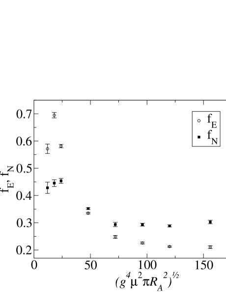
Figure 6.1: Left: The dependence of $f_{E}$ and $f_{N}$ on the field strength parameter $g^{2}\mu R_{A}$. Right: The dependence of $f_{E}$ and $f_{N}$ on lattice spacing for different values of $\mu$.

The energy and multiplicity, parametrized by the two dimensionless ratios

$$f_{E}=\frac{\,\mathrm{d}E/\,\mathrm{d}\eta}{g^{4}\mu^{3}\pi R_{A}^{2}}\quad\textrm{and}\quad f_{N}=\frac{\,\mathrm{d}N/\,\mathrm{d}\eta}{g^{2}\mu^{2}\pi R_{A}^{2}}$$ (6.1)

were calculated numerically using the method outlined in Sec. 5.1. These ratios were found to be approximately independent of the parameters of the calculation ($g$, $\mu$, $R_{A}$ and the lattice spacing $a$) in the strong field limit ($g^{2}\mu$ large enough), as can be seen from Fig. 6.1.

The values found in Ref. [1] were $f_{E}\approx 0.23$ and $f_{N}\approx 0.29$. These fit in with the two phenomenological scenarios outlined in Sec. 2.3 in the following way. Assuming a nuclear transverse area of $140\ \textrm{fm}^{2}$, $g=2$ and taking $g^{2}\mu=2.1\ \textrm{GeV}$ one gets

$$\frac{\,\mathrm{d}N^{\mathrm{init}}_{\mathrm{tot}}}{\,\mathrm{d}\eta}\approx 1100\quad\textrm{and}\quad\frac{\,\mathrm{d}E^{\mathrm{init}}_{T}}{\,\mathrm{d}\eta}\approx 1900\ \textrm{GeV},$$ (6.2)

which fits in well with the hydrodynamical expansion scenario outlined in Sec. 2.3. On the other hand a choice of $g^{2}\mu=1.4\ \textrm{GeV}$ would give

$$\frac{\,\mathrm{d}N^{\mathrm{init}}_{\mathrm{tot}}}{\,\mathrm{d}\eta}\approx 500\quad\textrm{and}\quad\frac{\,\mathrm{d}E^{\mathrm{init}}_{T}}{\,\mathrm{d}\eta}\approx 550\ \textrm{GeV},$$ (6.3)

which would be consistent with with the free streaming scenario, assuming a factor of 2 increase in the multiplicity from the scatterings of the partons and hadronization.

The CPU-time used for producing the results of Ref. [1] was of the order of a few thousand hours on a 2.4 GHz Pentium processor, with comparable amounts of computer resources used in the development phase of the code. The calculations were performed during the winter 2002-2003 using up to five 600 MHz Alpha EV6 processors in the “dynamo” minisupercluster at the Accelerator Laboratory and three desktop 2.4 GHz Pentium machines at the Theory Division, both at the University of Helsinki Department of Physics. The program consisted of approximately 7000 lines of code in ANSI C in addition to general purpose libraries for elementary complex number and SU(3)-matrix operations.

6.2 Rapidity dependence

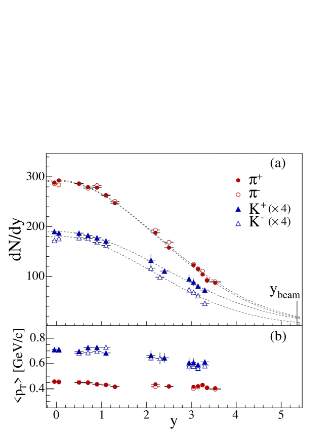
Figure 6.2: BRAHMS results on charged meason rapidity distributions in 5 % most central gold-gold collisions [204]. The dashed lines are Gaussian fits to the data with $\sigma_{\pi^{+}}=2.25\pm 0.02$ (stat) and $\sigma_{\pi^{-}}=2.29\pm 0.02$ (stat). The lower panel shows the mean transverse momentum of the mesons for different rapidities.

The calculations of Ref. [1] were further extended in Ref. [2]. The experimentally found rapidity (or $\ln 1/x$) dependence of the saturation scale discussed in Sec. 3.2 was exploited in a simple extension of the calculation of [1] to study the rapidity dependence of gluon production. The main assumption of the calculation was the following: in the fully boost invariant model described in Sec. 4.1 the only (implicit) dependence on rapidity comes though the strengths of the classical color sources $\rho_{(1,2)}$. It has been experimentally observed that the saturation scale varies with rapidity as $Q_{\mathrm{s}}^{2}(x)\sim{x}^{-\lambda}$. The saturation scale in the McLerran-Venugopalan model is proportional, up to a logarithm, to the source strength, $Q_{\mathrm{s}}\sim g^{2}\mu(\times\ln g^{2}\mu).$ It was argued in Ref. [2] that for central rapidities in heavy ion collisions the dominant ${x}$ scale that should be used to evaluate the saturation scale is given by ${x}_{1,2}\sim e^{\pm y}$ for the two nuclei. One can then study gluon production at the rapidity $y$ by choosing the source strengths as $g^{4}\mu^{2}\sim e^{\pm\lambda y}.$

The result of Ref. [2] was that the multiplicity of produced gluons can be described by very broad Gaussians in $y$ with width $\sigma\approx 6$. This kind of a Gaussian is much broader than the one observed at RHIC energies by the BRAHMS collaboration [204] (see Fig. 6.2), but coincidentally close to the pQCD+saturation model result [206, 207]. The conclusion suggested in Ref. [2] was then that at RHIC energies the rapidity dependence of particle production at central rapidities at AuAu-collisions at RHIC energies is not dominated by saturation physics. It is perhaps more dependent on the kind of high ${x}$ physics (the $(1-x)^{4}$-behavior of the gluon structure functions expected from momentum sum rules) incorporated e.g. in the “saturation model” calculations of Refs. [17, 93, 94] to reproduce the experimentally observed rapidity (or pseudorapidity) dependence.

The CPU-time used for producing the results of Ref. [2] was larger than what was used for Ref. [1] because the computations had to be done separately for different values of the rapidity. The total CPU-time was approximately 5000 hours on a 2.4 GHz Pentium processor. The calculations were performed during the late summer of 2004 mostly using three desktop 2.4 GHz Pentium machines at the Theory Division of the University of Helsinki Department of Physics.

6.3 Quark pair production: 1+1-dimensional toy model

In Ref. [3] the calculation of pair production by classical fields was formulated based on the theory detailed in Ref. [189] and closely following the calculation in the Abelian theory performed in Ref. [188]. It was then argued that the practical numerical solution of the Dirac equation in the forward light cone with the initial condition given at $\tau=0$ is most practically performed using as coodinates $\tau$ and $z$. The implicit discretization scheme required for this numerical solution was then constructed and demonstrated in a 1+1-dimensional toy model.

Figure 6.3: Diagrams contributing to the quark pair prodction amplitude in the 1+1-dimensional toy model.

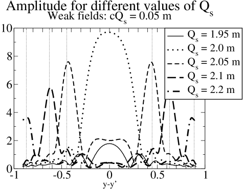
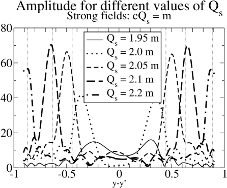
Figure 6.4: Absolute value of the quark pair production amplitude for different values of the oscillation scale $Q_{\mathrm{s}}$. Left: weak fields, the peaks are at the location given by the lowest order perturbative result. Right: strong fields with the same values of $Q_{\mathrm{s}}.$ Peaks near “threshold” $Q_{\mathrm{s}}=2m$ are shifted.

In the gauge $A_{\tau}=0$ that was used in calculating the classical background field the Dirac equation of the 1+1-dimensional toy model is

$$\partial_{\tau}\psi=\frac{\sqrt{\tau^{2}+z^{2}}+\gamma^{0}\gamma^{3}z}{\tau}\left(-\gamma^{0}\gamma^{3}\partial_{z}\psi-im_{\textrm{eff}}\gamma^{0}\psi\right)-i\gamma^{0}\gamma^{3}g\frac{A_{\eta}}{\tau}\psi.$$ (6.4)

The transverse coordinate dependence has been neglected and the mass of the 1+1-dimensional theory corresponds to the transverse mass of the full theory, $m^{2}_{\textrm{eff}}\approx{\mathbf{k}_{T}}^{2}+m^{2}$. The 1+1-dimensional toy model in the $A_{\tau}=0$-gauge only contains one component of the gauge field, $A_{\eta}$. In Ref. [3] this model was studied using two forms for the time dependence of this background field, an exponential decay and a Bessel function:

$$A_{\eta}=cQ_{\mathrm{s}}\tau J_{1}(Q_{\mathrm{s}}\tau).$$ (6.5)

This is the correct time dependence of the perturbative solution to the gauge field equations of motion [131].

For weak fields $c\ll 1$ the amplitude for quark pair production can be computed using the first order in perturbation theory (diagram (a) in Fig. 6.3). The result for the oscillating field of Eq. (6.5) is a peak at

$$2k^{+}k^{-}=(p+q)^{2}=2m_{\textrm{eff}}^{2}\left(1+\cosh(\Delta y)\right)=Q_{\mathrm{s}}^{2}.$$ (6.6)

As is demonstrated in Fig. 6.4, for weak fields the numerical computation of Ref. [3] reproduces this perturbative peak. For stronger fields the numerical solution sums over all the diagrams in Fig. 6.3 and the position of the peak is shifted. The appearence of this peak is not a physical effect. The time dependent field of Eq. (6.5) represents off-shell gluons with invariant mass $Q_{\mathrm{s}}^{2}$ decaying into quark pairs, and the amplitude has a peak where the invariant mass of the pair equals that of the gluon. In the full 3+1-dimensional case the gluons are on shell, and this peak is washed out by integration over the relative transverse momentum of the pair. The effect serves here as a verification that the numerical method for solving the Dirac equation and projecting out the positive energy solutions works.

Chapter 7 Review and outlook

The classical field approximation is a theoretically appealing way to study QCD as it manifests itself in the small ${x}$ proton or nucleus wavefunction and in relativistic heavy ion collisions. The aim of this thesis has been to review how a classical field model can be used to understand the initial stages of a heavy ion collision towards thermalization, starting from a model of the nuclear wavefunction. It has been seen that the classical field model gives a plausible picture of gluon production in the central rapidity region of a heavy ion collision. One can numerically calculate the gluon multiplicity and transverse energy created in the initial stages of the collision. This calculation was the subject of the first article of this thesis [1], and it was shown that the values obtained are compatible with experimental observations within the Bjorken scenario of boost invariant ideal hydrodynamical expansion.

Due to the uncertainty of the appropriate value of the source charge density the results of the classical model do not, however, rule out a free-streaming scenario without the decrease of energy density due to $p\,\mathrm{d}V$-work in the hydronynamical evolution. This uncertainty can be reduced in two ways. Firstly observations of the hadron suppression at large $p_{T}$, the disappearence of away-side jet-like correlations and elliptic flow favor the interpretation in terms of the Bjorken scenario, although hydrodynamical models do have difficulties with HBT radii and there have been attempts to explain elliptic flow without referring to hydrodynamics [209, 137]. Secondly one should in principle be able to independently determine the value of the source strength parameter using data from deep inelastic scattering. Doing this accurately enough to clearly distinguish between $g^{2}\mu=1.4\ \textrm{GeV}$ and $g^{2}\mu=2.1\ \textrm{GeV}$ is, however, not easy.

Inclusion of the longitudinal dimension is important for fully understanding two seemingly unrelated issues. One is the thermalization, or specifically the isotropisation, of the initial gluonic system. The essential assumption of the hydrodynamical model is that the thermal system is isotropic, i.e. has not only transverse but also longitudinal pressure. Explaining the creation of longitudinal pressure, if it can be done in the classical field model, must necessarily involve a full 3+1-dimensional solution of the gauge field equations of motion. The second issue that requires a better treatment of the longitudinal dimension is including the effects of JIMWLK evolution. The approach used in the second article of the present thesis [2], consists of varying the initial conditions of the same 2+1-dimensional calculation to account for the change in the saturation scale at different rapidities. There exists a large body of both analytical and numerical work on this equation, which is not yet fully included in this simple approach.

The question of theoretically understanding of the thermal and chemical equilibration that the experimental results seem to indicate is not as well understood. In the third article of this thesis we have formulated a way to calculate the number of quark pairs produced in the classical field model. The calculation essentially consists of solving the Dirac equation in the background given by the classical gauge fields. Many technical issues concerning, in particular, the longitudinal dimension have been solved in a 1+1-dimensional toy model. The full 3+1-dimensional case, requiring an extensive numerical calculation, has been formulated but not yet implemented numerically.

Acknowledgements

I want to thank K. Kajantie for directing me to this direction of research and advice, K. J. Eskola, F. Gelis and K. Rummukainen for reading this manuscript, and P. Hoyer and P.V. Ruuskanen for discussions. This work has been supported by the Finnish Cultural Foundation and the Magnus Ehrnrooth Foundation as well as the Helsinki Institute of Physics and the Academy of Finland, contract no. 77744.

Appendix A Notations

A.1 Spacetime

The metric in the original $\{t,z,\mathbf{x}_{T}\}$-basis is $g_{\mu\nu}=\textrm{diag}(1,-1,-1,-1).$ Thus $\partial_{i}\partial^{i}=-\partial_{i}\partial_{i}=-\boldsymbol{\nabla}_{T}^{2}$. We define the light cone coordinates $x^{\pm}$ and proper time and spacetime rapidity $\tau,\eta$ as:

$$x^{\pm} = \frac{1}{\sqrt{2}}(t\pm z) = \frac{1}{\sqrt{2}}\tau e^{\pm\eta}$$ (A.1)

$$\tau = \sqrt{t^{2}-z^{2}} = \sqrt{2x^{+}x^{-}}$$

$$\eta = \frac{1}{2}\ln{\frac{t+z}{t-z}} = \frac{1}{2}\ln{\frac{x^{+}}{x^{-}}},$$

which gives the original coordinates in terms of the new ones as

$$t = \frac{1}{\sqrt{2}}(x^{+}+x^{-}) = \tau\cosh{\eta}$$ (A.2)

$$z = \frac{1}{\sqrt{2}}(x^{+}-x^{-}) = \tau\sinh{\eta}.$$

The metric in the light cone coordinates is $\,\mathrm{d}s^{2}=2\,\mathrm{d}x^{+}x^{-}-\,\mathrm{d}\mathbf{x}_{T}^{2}$ and the $\tau,\eta$ coordinates $\,\mathrm{d}s^{2}=\,\mathrm{d}\tau^{2}-\tau^{2}\,\mathrm{d}\eta^{2}-\,\mathrm{d}\mathbf{x}_{T}^{2},$ giving the invariant integration measure $\sqrt{|g|}\,\mathrm{d}^{4}x=\,\mathrm{d}z\,\mathrm{d}t\,\mathrm{d}^{2}\mathbf{x}_{T}=\,\mathrm{d}x^{+}\,\mathrm{d}x^{-}\,\mathrm{d}^{2}\mathbf{x}_{T}=\tau\,\mathrm{d}\eta\,\mathrm{d}\tau\,\mathrm{d}^{2}\mathbf{x}_{T}.$ Any vector, in particular the gauge field $A_{\mu}$, transforms under coordinate transformations in the familiar way

$$A^{\mu^{\prime}}=\frac{\partial x^{\mu^{\prime}}}{\partial x^{\mu}}A^{\mu}\quad A_{\mu^{\prime}}=\frac{\partial x^{\mu}}{\partial x^{\mu^{\prime}}}A_{\mu}.$$ (A.3)

Straightforward application of Eq. (A.3) gives the $\tau,\eta$-components of a vector as

$$A_{\tau} = A^{\tau} = (x^{+}A^{-}+x^{-}A^{+})/\tau$$ (A.4)

$$A_{\eta} = -\tau^{2}A^{\eta} = x^{+}A^{-}-x^{-}A^{+}.$$

A.2 Chromodynamics

We denote the generators of the fundamental representation of the gauge group by $t_{a}$. They are related to the Gell-Mann matrices $\lambda^{a}$ and the Pauli matrices $\sigma^{a}$ by $t_{a}=\lambda^{a}/2$ for ${N_{\mathrm{c}}}=3$ and $t_{a}=\sigma_{a}/2$ for ${N_{\mathrm{c}}}=2$. The generators are normalized as

$$\operatorname{Tr}t_{a}t_{b}=\frac{1}{2}\delta_{ab}$$ (A.5)

$$[t_{a},t_{b}]=if_{abc}t_{c}.$$ (A.6)

The structure constants are completely antisymmetric in their indices [210]. The color indices $a,b,c,\dots$ range from 1 to ${N_{\mathrm{c}}}^{2}-1$, the dimension of the group. They are written here indifferently as superscripts or subscripts. The adjoint representation is generated by $(T_{a})_{bc}=-if_{abc}$.

$$\operatorname{Tr}T_{a}T_{b}={N_{\mathrm{c}}}\delta_{ab},\textrm{ or }T_{a}T_{a}={N_{\mathrm{c}}}\mathbf{1}_{({N_{\mathrm{c}}}^{2}-1)},$$ (A.7)

where $\mathbf{1}_{({N_{\mathrm{c}}}^{2}-1)}$ is the $({N_{\mathrm{c}}}^{2}-1)\times({N_{\mathrm{c}}}^{2}-1)$ identity matrix. The adjoint representation of an SU(${N_{\mathrm{c}}}$)-matrix $U=\exp{i\chi^{a}t_{a}}$ is denoted by $D_{\mathrm{adj}}(U)\equiv\exp{i\chi^{a}T_{a}}$, and is related to the fundamental representation by

$$2\operatorname{Tr}(t_{a}U^{\dagger}t_{b}U)=(D_{\mathrm{adj}}(U))_{ab}.$$ (A.8)

We use the following notation for the dimensions and the Casimirs of the representations:

$$\begin{array}[]{rclcrcl}d_{\mathrm{F}}&=&{N_{\mathrm{c}}}&&d_{\mathrm{A}}&=&{N_{\mathrm{c}}}^{2}-1\\ C_{\mathrm{F}}&=&\frac{{N_{\mathrm{c}}}^{2}-1}{2{N_{\mathrm{c}}}}&&C_{\mathrm{A}}&=&{N_{\mathrm{c}}}\\ \end{array}$$ (A.9)

The action of QCD is

$$S=\int\!\,\mathrm{d}^{4}x\sum_{f}\bar{\psi}_{f}(iD\!\!\!\!/\!-m)\psi_{f},-\frac{1}{2}\operatorname{Tr}F^{\mu\nu}F_{\mu\nu}$$ (A.10)

with the covariant derivative

$$D^{\mu}=\partial^{\mu}+igA^{\mu},$$ (A.11)

giving the fields trength tensor

$$F^{\mu\nu}=-\frac{i}{g}[D^{\mu},D^{\nu}]=\partial^{\mu}A^{\nu}-\partial^{\nu}A^{\mu}+ig[A^{\mu},A^{\nu}]$$ (A.12)

or in components

$$F^{\mu\nu}_{a}=\partial^{\mu}A^{\nu}_{a}-\partial^{\nu}A^{\mu}_{a}-gf^{abc}A^{\mu}_{b}A^{\nu}_{c}.$$ (A.13)

QCD is invariant under gauge transformations, parametrized by a spacetime dependent matrix in the gauge group, $U(x)$:

$$A^{\mu}\to UA^{\mu}U^{\dagger}-\frac{i}{g}U\partial^{\mu}U^{\dagger}.$$ (A.14)

Under these transformations the covariant derivative and the field strength tensor transform as

$$D^{\mu}\to UD^{\mu}U^{\dagger}\ \textrm{ and }\ F^{\mu\nu}\to UF^{\mu\nu}U^{\dagger}.$$ (A.15)

A field configuration that is gauge equivalent to the vacuum is called a pure gauge:

$$A^{\mu}=-\frac{i}{g}U\partial^{\mu}U^{\dagger}.$$ (A.16)

A.3 Gauge fields on the lattice

Figure A.1: The link matrix $U_{\mu}(x)$ connects the lattice site $x$ to $x+\!e_{\mu}\!$ (left). The Hermitian conjugate $U^{\dagger}_{\nu}(x)$ connects lattice points in the negative direction, going from $x+\!e_{\nu}\!$ to $x$.

The fundamental object of lattice gauge field theory is the link matrix $U_{\mu}(x)$ connecting the point $x$ to the neighboring lattice site $x+e_{\mu}$ (see Fig. A.1). The Hermitian conjugate of the link matrix reverses the direction, connecting $x+e_{\mu}$ to $x.$ In terms of the continuum gauge field $A_{\mu}$ we identify the link matrix as $U_{\mu}(x)=e^{igaA_{\mu}(x)}$

A gauge transformation on the lattice transforms the link matrices as

$$U_{\mu}(x)\to V(x)U_{\mu}(x)V^{\dagger}(x\!+\!e_{\mu}\!),$$ (A.17)

and the fermion fields as

$$\psi(x)\to V(x)\psi(x),\quad\bar{\psi}(x)\to\bar{\psi}(x)V^{\dagger},$$ (A.18)

leaving the following combination gauge-invariant

$$\bar{\psi}(x)\gamma^{\mu}U_{\mu}(x)\psi(x\!+\!e_{\mu}\!).$$ (A.19)

A pure gauge field is one that can be gauge transformed to zero, meaning that the link matrices can be transformed to the indentity matrix:

$$U_{\mu}(x)=V(x)V^{\dagger}(x\!+\!e_{\mu}\!).$$ (A.20)

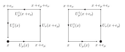
Figure A.2: The plaquettes $U_{\mu,\nu}(x)$ (left) and $U_{\nu,-\mu}(x+\!e_{\mu}\!)$ (right) circle the same contour, but gauge transform on different points, $x$ and $x+\!e_{\mu}\!$ respectively.

A gauge invariant action can be defined using the plaquette

$$U_{\mu,\nu}(x)=U_{\mu}(x)U_{\nu}(x\!+\!e_{\mu}\!)U^{\dagger}_{\mu}(x\!+\!e_{\nu}\!)U^{\dagger}_{\nu}(x).$$ (A.21)

With a subscript $-\mu$ we denote the negative $\mu$-direction. Thus a plaquette around the same contour, but based on a different point (see Fig. A.2) can be written e.g. as

$$U_{\nu,-\mu}(x+\!e_{\mu}\!)=U_{\nu}(x\!+\!e_{\mu}\!)U^{\dagger}_{\mu}(x\!+\!e_{\nu}\!)U^{\dagger}_{\nu}(x)U_{\mu}(x).$$ (A.22)

As can be seen from its definition and the transformation properties of the link matrices, the plaquette gauge transforms at its base point

$$U_{\mu,\nu}(x)\to V(x)U_{\mu,\nu}(x)V^{\dagger}(x).$$ (A.23)

Because of cyclicity, the trace of the plaquette is gauge invariant and independent of the base point

$$\operatorname{Tr}U_{\mu,\nu}(x)=\operatorname{Tr}U_{\nu,-\mu}(x+\!e_{\mu}\!)=\operatorname{Tr}U_{-\mu,-\nu}(x+\!e_{\mu}\!+\!e_{\nu}\!)=\operatorname{Tr}U_{-\nu,\mu}(x+\!e_{\nu}\!).$$ (A.24)

In the continuum limit the plaquette becomes

$$U_{\mu,\nu}=e^{iga^{2}F_{\mu\nu}+\mathcal{O}(a^{3})}.$$ (A.25)

and the pure gauge action $S=-\frac{1}{2}\operatorname{Tr}F_{\mu\nu}^{2}$ can be represented by the Wilson action [211]

$$S=-\frac{2{N_{\mathrm{c}}}}{g^{2}}\sum_{x}\sum_{\mu<\nu}\left(1-\frac{1}{{N_{\mathrm{c}}}}\mathrm{Re}\ \operatorname{Tr}U_{\mu,\nu}\right).$$ (A.26)

In Minkowski space one must choose a different sign for the $0,i$-terms to reproduce the right metric.

Bibliography

- [1] T. Lappi, Phys. Rev. C67, 054903 (2003), [hep-ph/0303076].
- [2] T. Lappi, Phys. Rev. C70, 054905 (2004), [hep-ph/0409328].
- [3] F. Gelis, K. Kajantie and T. Lappi, Phys. Rev. C71, 024904 (2005), [hep-ph/0409058].
- [4] STAR, J. Adams et al., nucl-ex/0501009.
- [5] PHENIX, K. Adcox et al., nucl-ex/0410003.
- [6] BRAHMS, I. Arsene et al., nucl-ex/0410020.
- [7] PHOBOS, B. B. Back et al., nucl-ex/0410022.
- [8] A. Freund, K. Rummukainen, H. Weigert and A. Schafer, Phys. Rev. Lett. 90, 222002 (2003), [hep-ph/0210139].
- [9] PHENIX, K. Adcox et al., Phys. Rev. Lett. 88, 242301 (2002), [nucl-ex/0112006].
- [10] PHENIX, S. S. Adler et al., Phys. Rev. Lett. 91, 172301 (2003), [nucl-ex/0305036].
- [11] PHENIX, S. S. Adler et al., Phys. Rev. C69, 034909 (2004), [nucl-ex/0307022].
- [12] R. J. Fries, J. Phys. G30, S853 (2004), [nucl-th/0403036].
- [13] H. Ehtamo, J. Lindfors and L. D. McLerran, Z. Phys. C18, 341 (1983).
- [14] L. D. McLerran and R. Venugopalan, Phys. Rev. D49, 2233 (1994), [hep-ph/9309289].
- [15] L. D. McLerran and R. Venugopalan, Phys. Rev. D49, 3352 (1994), [hep-ph/9311205].
- [16] L. D. McLerran and R. Venugopalan, Phys. Rev. D50, 2225 (1994), [hep-ph/9402335].
- [17] D. Kharzeev and E. Levin, Phys. Lett. B523, 79 (2001), [nucl-th/0108006].
- [18] D. Kharzeev, E. Levin and L. McLerran, Phys. Lett. B561, 93 (2003), [hep-ph/0210332].
- [19] D. Kharzeev, Y. V. Kovchegov and K. Tuchin, Phys. Rev. D68, 094013 (2003), [hep-ph/0307037].
- [20] D. Kharzeev, E. Levin and M. Nardi, hep-ph/0408050.
- [21] D. Kharzeev, E. Levin and M. Nardi, Nucl. Phys. A730, 448 (2004), [hep-ph/0212316].
- [22] J. P. Blaizot, F. Gelis and R. Venugopalan, hep-ph/0402256.
- [23] J. P. Blaizot, F. Gelis and R. Venugopalan, hep-ph/0402257.
- [24] D. Kharzeev and K. Tuchin, Nucl. Phys. A735, 248 (2004), [hep-ph/0310358].
- [25] A. Krasnitz and R. Venugopalan, Nucl. Phys. B557, 237 (1999), [hep-ph/9809433].
- [26] S. A. Bass et al., Nucl. Phys. A661, 205 (1999), [nucl-th/9907090].
- [27] T. Lappi, hep-ph/0409087.
- [28] M. Gyulassy and L. McLerran, nucl-th/0405013.
- [29] J.-P. Blaizot and F. Gelis, hep-ph/0405305.
- [30] J. D. Bjorken, Phys. Rev. D27, 140 (1983).
- [31] J. P. Blaizot and A. H. Mueller, Nucl. Phys. B289, 847 (1987).
- [32] J.-P. Blaizot, E. Iancu and A. Rebhan, hep-ph/0303185.
- [33] J. L. Nagle and T. S. Ullrich, nucl-ex/0203007.
- [34] J. Schukraft, Lectures at the Cargese Summer School on QCD Perspectives on Hot and Dense Matter, Cargese, France, 6-18 Aug 2001.
- [35] J. Schukraft, Nucl. Phys. A698, 287 (2002).
- [36] STAR, J. Adams et al., Phys. Rev. Lett. 91, 072304 (2003), [nucl-ex/0306024].
- [37] PHENIX, S. S. Adler et al., Phys. Rev. Lett. 91, 072303 (2003), [nucl-ex/0306021].
- [38] BRAHMS, I. Arsene et al., nucl-ex/0403005.
- [39] PHOBOS, B. B. Back et al., Phys. Rev. Lett. 91, 072302 (2003), [nucl-ex/0306025].
- [40] R. Baier, A. Kovner and U. A. Wiedemann, Phys. Rev. D68, 054009 (2003), [hep-ph/0305265].
- [41] D. Kharzeev, E. Levin and L. McLerran, hep-ph/0403271.
- [42] D. Kharzeev, Y. V. Kovchegov and K. Tuchin, hep-ph/0405045.
- [43] M. Gyulassy, I. Vitev, X.-N. Wang and B.-W. Zhang, nucl-th/0302077.
- [44] STAR, C. Adler et al., Phys. Rev. Lett. 90, 082302 (2003), [nucl-ex/0210033].
- [45] PHENIX, S. S. Adler et al., nucl-ex/0408007.
- [46] P. Braun-Munzinger, K. Redlich and J. Stachel, nucl-th/0304013.
- [47] F. Becattini, Z. Phys. C69, 485 (1996).
- [48] F. Becattini and U. W. Heinz, Z. Phys. C76, 269 (1997), [hep-ph/9702274].
- [49] F. Becattini and G. Passaleva, Eur. Phys. J. C23, 551 (2002), [hep-ph/0110312].
- [50] P. Blanchard, S. Fortunato and H. Satz, Eur. Phys. J. C34, 361 (2004), [hep-ph/0401103].
- [51] STAR, J. Adams et al., nucl-ex/0409033.
- [52] P. Huovinen, P. F. Kolb, U. W. Heinz, P. V. Ruuskanen and S. A. Voloshin, Phys. Lett. B503, 58 (2001), [hep-ph/0101136].
- [53] P. F. Kolb and R. Rapp, Phys. Rev. C67, 044903 (2003), [hep-ph/0210222].
- [54] P. F. Kolb, nucl-th/0407066.
- [55] P. F. Kolb, J. Sollfrank and U. W. Heinz, Phys. Rev. C62, 054909 (2000), [hep-ph/0006129].
- [56] F. Retiere and M. A. Lisa, nucl-th/0312024.
- [57] K. J. Eskola, H. Niemi, P. V. Ruuskanen and S. S. Rasanen, Phys. Lett. B566, 187 (2003), [hep-ph/0206230].
- [58] D. Magestro, nucl-ex/0408014.
- [59] G. Aarts and J. Smit, Nucl. Phys. B555, 355 (1999), [hep-ph/9812413].
- [60] M. Salle, J. Smit and J. C. Vink, Phys. Rev. D64, 025016 (2001), [hep-ph/0012346].
- [61] M. Salle, J. Smit and J. C. Vink, Nucl. Phys. B625, 495 (2002), [hep-ph/0012362].
- [62] M. Salle, Phys. Rev. D69, 025005 (2004), [hep-ph/0307080].
- [63] J. Berges, S. Borsanyi and J. Serreau, Nucl. Phys. B660, 51 (2003), [hep-ph/0212404].
- [64] J. Berges and J. Serreau, Phys. Rev. Lett. 91, 111601 (2003), [hep-ph/0208070].
- [65] G. Aarts, D. Ahrensmeier, R. Baier, J. Berges and J. Serreau, Phys. Rev. D66, 045008 (2002), [hep-ph/0201308].
- [66] J. Berges, hep-ph/0409233.
- [67] J. Berges, hep-ph/0401172.
- [68] R. Baier, A. H. Mueller, D. Schiff and D. T. Son, Phys. Lett. B502, 51 (2001), [hep-ph/0009237].
- [69] P. Arnold, J. Lenaghan and G. D. Moore, JHEP 08, 002 (2003), [hep-ph/0307325].
- [70] D. M. Elliott and D. H. Rischke, Nucl. Phys. A671, 583 (2000), [nucl-th/9908004].
- [71] P. Arnold and J. Lenaghan, hep-ph/0408052.
- [72] P. Arnold, hep-ph/0409002.
- [73] P. Arnold, J. Lenaghan, G. D. Moore and L. G. Yaffe, nucl-th/0409068.
- [74] P. Romatschke and M. Strickland, Phys. Rev. D68, 036004 (2003), [hep-ph/0304092].
- [75] P. Romatschke and M. Strickland, hep-ph/0406188.
- [76] P. Romatschke and M. Strickland, hep-ph/0408275.
- [77] P. Romatschke and M. Strickland, hep-ph/0408314.
- [78] P. Arnold, G. D. Moore and L. G. Yaffe, JHEP 11, 001 (2000), [hep-ph/0010177].
- [79] P. Arnold, G. D. Moore and L. G. Yaffe, JHEP 05, 051 (2003), [hep-ph/0302165].
- [80] G. Policastro, D. T. Son and A. O. Starinets, Phys. Rev. Lett. 87, 081601 (2001), [hep-th/0104066].
- [81] X.-N. Wang and M. Gyulassy, Phys. Rev. D44, 3501 (1991).
- [82] PHENIX, K. Adcox et al., Phys. Rev. Lett. 87, 052301 (2001), [nucl-ex/0104015].
- [83] STAR, C. Adler et al., Phys. Rev. Lett. 87, 112303 (2001), [nucl-ex/0106004].
- [84] PHOBOS, B. B. Back et al., Phys. Rev. Lett. 87, 102303 (2001), [nucl-ex/0106006].
- [85] BRAHMS, I. G. Bearden et al., Phys. Lett. B523, 227 (2001), [nucl-ex/0108016].
- [86] BRAHMS, I. G. Bearden et al., Phys. Rev. Lett. 88, 202301 (2002), [nucl-ex/0112001].
- [87] PHOBOS, B. B. Back et al., Phys. Rev. C65, 061901 (2002), [nucl-ex/0201005].
- [88] PHENIX, S. S. Adler et al., nucl-ex/0409015.
- [89] STAR, J. Adams et al., nucl-ex/0407003.
- [90] U. W. Heinz and S. M. H. Wong, Phys. Rev. C66, 014907 (2002), [hep-ph/0205058].
- [91] K. J. Eskola, K. Kajantie, P. V. Ruuskanen and K. Tuominen, Nucl. Phys. B570, 379 (2000), [hep-ph/9909456].
- [92] K. J. Eskola, P. V. Ruuskanen, S. S. Rasanen and K. Tuominen, Nucl. Phys. A696, 715 (2001), [hep-ph/0104010].
- [93] T. Hirano and Y. Nara, nucl-th/0403029.
- [94] T. Hirano and Y. Nara, nucl-th/0404039.
- [95] D. Kharzeev and M. Nardi, Phys. Lett. B507, 121 (2001), [nucl-th/0012025].
- [96] V. A. Khoze and W. Ochs, Int. J. Mod. Phys. A12, 2949 (1997), [hep-ph/9701421].
- [97] A. H. Mueller, Nucl. Phys. B572, 227 (2000), [hep-ph/9906322].
- [98] ZEUS, J. Breitweg et al., Eur. Phys. J. C7, 609 (1999), [hep-ex/9809005].
- [99] ZEUS, S. Chekanov et al., Phys. Rev. D67, 012007 (2003), [hep-ex/0208023].
- [100] L. V. Gribov, E. M. Levin and M. G. Ryskin, Phys. Rept. 100, 1 (1983).
- [101] A. H. Mueller and J.-W. Qiu, Nucl. Phys. B268, 427 (1986).
- [102] A. H. Mueller, Nucl. Phys. B558, 285 (1999), [hep-ph/9904404].
- [103] K. J. Eskola, H. Honkanen, V. J. Kolhinen, J.-w. Qiu and C. A. Salgado, Nucl. Phys. B660, 211 (2003), [hep-ph/0211239].
- [104] K. J. Eskola, V. J. Kolhinen and R. Vogt, J. Phys. G30, S1171 (2004), [hep-ph/0403130].
- [105] K. Golec-Biernat and M. Wusthoff, Phys. Rev. D59, 014017 (1999), [hep-ph/9807513].
- [106] K. Golec-Biernat and M. Wusthoff, Phys. Rev. D60, 114023 (1999), [hep-ph/9903358].
- [107] A. H. Mueller, Nucl. Phys. B415, 373 (1994).
- [108] A. H. Mueller, Nucl. Phys. B437, 107 (1995), [hep-ph/9408245].
- [109] A. H. Mueller and B. Patel, Nucl. Phys. B425, 471 (1994), [hep-ph/9403256].
- [110] B. Andersson, G. Gustafson, A. Nilsson and C. Sjogren, Z. Phys. C49, 79 (1991).
- [111] N. N. Nikolaev and B. G. Zakharov, Z. Phys. C49, 607 (1991).
- [112] M. McDermott, L. Frankfurt, V. Guzey and M. Strikman, Eur. Phys. J. C16, 641 (2000), [hep-ph/9912547].
- [113] S. J. Brodsky, P. Hoyer, N. Marchal, S. Peigne and F. Sannino, Phys. Rev. D65, 114025 (2002), [hep-ph/0104291].
- [114] S. J. Brodsky, R. Enberg, P. Hoyer and G. Ingelman, hep-ph/0409119.
- [115] ZEUS, M. Derrick et al., Z. Phys. C69, 607 (1996), [hep-ex/9510009].
- [116] H1, S. Aid et al., Nucl. Phys. B470, 3 (1996), [hep-ex/9603004].
- [117] ZEUS, M. Derrick et al., Z. Phys. C72, 399 (1996), [hep-ex/9607002].
- [118] H1, C. Adloff et al., Nucl. Phys. B497, 3 (1997), [hep-ex/9703012].
- [119] ZEUS, J. Breitweg et al., Phys. Lett. B407, 432 (1997), [hep-ex/9707025].
- [120] H1, C. Adloff et al., Z. Phys. C76, 613 (1997), [hep-ex/9708016].
- [121] ZEUS, J. Breitweg et al., Eur. Phys. J. C1, 81 (1998), [hep-ex/9709021].
- [122] ZEUS, J. Breitweg et al., Eur. Phys. J. C6, 43 (1999), [hep-ex/9807010].
- [123] A. M. Stasto, K. Golec-Biernat and J. Kwiecinski, Phys. Rev. Lett. 86, 596 (2001), [hep-ph/0007192].
- [124] E665, M. R. Adams et al., Z. Phys. C67, 403 (1995), [hep-ex/9505006].
- [125] E665, M. R. Adams et al., Z. Phys. C65, 225 (1995).
- [126] New Muon, M. Arneodo et al., Nucl. Phys. B487, 3 (1997), [hep-ex/9611022].
- [127] S. K. Wong, Nuovo Cim. A65, 689 (1970).
- [128] Y. V. Kovchegov, Phys. Rev. D54, 5463 (1996), [hep-ph/9605446].
- [129] Y. V. Kovchegov, Phys. Rev. D55, 5445 (1997), [hep-ph/9701229].
- [130] A. Kovner, L. D. McLerran and H. Weigert, Phys. Rev. D52, 6231 (1995), [hep-ph/9502289].
- [131] A. Kovner, L. D. McLerran and H. Weigert, Phys. Rev. D52, 3809 (1995), [hep-ph/9505320].
- [132] J. Jalilian-Marian, A. Kovner, L. D. McLerran and H. Weigert, Phys. Rev. D55, 5414 (1997), [hep-ph/9606337].
- [133] J. Jalilian-Marian, S. Jeon and R. Venugopalan, Phys. Rev. D63, 036004 (2001), [hep-ph/0003070].
- [134] S. Jeon and R. Venugopalan, hep-ph/0406169.
- [135] C. S. Lam and G. Mahlon, Phys. Rev. D61, 014005 (2000), [hep-ph/9907281].
- [136] C. S. Lam and G. Mahlon, Phys. Rev. D64, 016004 (2001), [hep-ph/0102337].
- [137] A. Krasnitz, Y. Nara and R. Venugopalan, Phys. Lett. B554, 21 (2003), [hep-ph/0204361].
- [138] A. Krasnitz, Y. Nara and R. Venugopalan, Nucl. Phys. A717, 268 (2003), [hep-ph/0209269].
- [139] M. Gyulassy and L. D. McLerran, Phys. Rev. C56, 2219 (1997), [nucl-th/9704034].
- [140] C. S. Lam and G. Mahlon, Phys. Rev. D62, 114023 (2000), [hep-ph/0007133].
- [141] J. Jalilian-Marian, A. Kovner, A. Leonidov and H. Weigert, Nucl. Phys. B504, 415 (1997), [hep-ph/9701284].
- [142] J. Jalilian-Marian, A. Kovner, A. Leonidov and H. Weigert, Phys. Rev. D59, 014014 (1999), [hep-ph/9706377].
- [143] J. Jalilian-Marian, A. Kovner and H. Weigert, Phys. Rev. D59, 014015 (1999), [hep-ph/9709432].
- [144] H. Weigert, Nucl. Phys. A703, 823 (2002), [hep-ph/0004044].
- [145] E. Iancu, A. Leonidov and L. D. McLerran, Phys. Lett. B510, 133 (2001), [hep-ph/0102009].
- [146] A. H. Mueller, Phys. Lett. B523, 243 (2001), [hep-ph/0110169].
- [147] E. Iancu and L. D. McLerran, Phys. Lett. B510, 145 (2001), [hep-ph/0103032].
- [148] E. Iancu, K. Itakura and L. McLerran, Nucl. Phys. A724, 181 (2003), [hep-ph/0212123].
- [149] E. Iancu, K. Itakura and L. McLerran, Nucl. Phys. A708, 327 (2002), [hep-ph/0203137].
- [150] J.-P. Blaizot, E. Iancu and H. Weigert, Nucl. Phys. A713, 441 (2003), [hep-ph/0206279].
- [151] K. Rummukainen and H. Weigert, Nucl. Phys. A739, 183 (2004), [hep-ph/0309306].
- [152] E. Iancu, A. Leonidov and L. McLerran, hep-ph/0202270.
- [153] E. Iancu and R. Venugopalan, hep-ph/0303204.
- [154] I. Balitsky, Nucl. Phys. B463, 99 (1996), [hep-ph/9509348].
- [155] W. Buchmuller, M. F. McDermott and A. Hebecker, Nucl. Phys. B487, 283 (1997), [hep-ph/9607290].
- [156] W. Buchmuller, T. Gehrmann and A. Hebecker, Nucl. Phys. B537, 477 (1999), [hep-ph/9808454].
- [157] A. H. Mueller, hep-ph/0111244.
- [158] R. V. Gavai and R. Venugopalan, Phys. Rev. D54, 5795 (1996), [hep-ph/9605327].
- [159] Y. V. Kovchegov, Phys. Rev. D60, 034008 (1999), [hep-ph/9901281].
- [160] C. S. Lam, G. Mahlon and W. Zhu, Phys. Rev. D66, 074005 (2002), [hep-ph/0207058].
- [161] A. Kovner, J. G. Milhano and H. Weigert, Phys. Rev. D62, 114005 (2000), [hep-ph/0004014].
- [162] Y. V. Kovchegov, Nucl. Phys. A692, 557 (2001), [hep-ph/0011252].
- [163] N. Armesto, M. A. Braun, E. G. Ferreiro and C. Pajares, Phys. Rev. Lett. 77, 3736 (1996), [hep-ph/9607239].
- [164] M. Nardi and H. Satz, Phys. Lett. B442, 14 (1998), [hep-ph/9805247].
- [165] H. Satz, hep-ph/0212046.
- [166] S. Digal, S. Fortunato, P. Petreczky and H. Satz, Phys. Lett. B549, 101 (2002), [hep-ph/0207264].
- [167] S. Digal, S. Fortunato and H. Satz, Eur. Phys. J. C32, 547 (2004), [hep-ph/0310354].
- [168] A. Dumitru and L. D. McLerran, Nucl. Phys. A700, 492 (2002), [hep-ph/0105268].
- [169] Y. V. Kovchegov and D. H. Rischke, Phys. Rev. C56, 1084 (1997), [hep-ph/9704201].
- [170] Y. V. Kovchegov and A. H. Mueller, Nucl. Phys. B529, 451 (1998), [hep-ph/9802440].
- [171] A. Makhlin, hep-ph/9608259.
- [172] A. Makhlin, hep-ph/9608261.
- [173] A. Makhlin and E. Surdutovich, Phys. Rev. C58, 389 (1998), [hep-ph/9803364].
- [174] A. Makhlin, Phys. Rev. C63, 044902 (2001), [hep-ph/0007300].
- [175] A. Makhlin, Phys. Rev. C63, 044903 (2001), [hep-ph/0007301].
- [176] A. Makhlin and E. Surdutovich, Phys. Rev. C63, 044904 (2001), [hep-ph/0007302].
- [177] A. Makhlin, hep-ph/0009067.
- [178] J. F. Gunion and G. Bertsch, Phys. Rev. D25, 746 (1982).
- [179] K. J. Eskola and K. Kajantie, Z. Phys. C75, 515 (1997), [nucl-th/9610015].
- [180] F. Gelis and R. Venugopalan, Phys. Rev. D69, 014019 (2004), [hep-ph/0310090].
- [181] E. Shuryak and I. Zahed, Phys. Rev. D67, 014006 (2003), [hep-ph/0206022].
- [182] K. Kajantie and T. Matsui, Phys. Lett. B164, 373 (1985).
- [183] G. Gatoff, A. K. Kerman and T. Matsui, Phys. Rev. D36, 114 (1987).
- [184] Y. Kluger, J. M. Eisenberg, B. Svetitsky, F. Cooper and E. Mottola, Phys. Rev. D45, 4659 (1992).
- [185] F. Cooper, J. M. Eisenberg, Y. Kluger, E. Mottola and B. Svetitsky, Phys. Rev. D48, 190 (1993), [hep-ph/9212206].
- [186] D. D. Dietrich, Phys. Rev. D68, 105005 (2003), [hep-th/0302229].
- [187] D. D. Dietrich, hep-th/0402026.
- [188] A. J. Baltz and L. D. McLerran, Phys. Rev. C58, 1679 (1998), [nucl-th/9804042].
- [189] A. J. Baltz, F. Gelis, L. D. McLerran and A. Peshier, Nucl. Phys. A695, 395 (2001), [nucl-th/0101024].
- [190] N. D. Birrell and P. C. W. Davies, Quantum fields in curved space (Cambridge University Press, 1982).
- [191] A. Krasnitz and R. Venugopalan, Phys. Rev. Lett. 86, 1717 (2001), [hep-ph/0007108].
- [192] A. Krasnitz and R. Venugopalan, Phys. Rev. Lett. 84, 4309 (2000), [hep-ph/9909203].
- [193] A. Krasnitz, Y. Nara and R. Venugopalan, Phys. Rev. Lett. 87, 192302 (2001), [hep-ph/0108092].
- [194] A. Krasnitz, Y. Nara and R. Venugopalan, Nucl. Phys. A727, 427 (2003), [hep-ph/0305112].
- [195] J. Jalilian-Marian, Y. Nara and R. Venugopalan, Phys. Lett. B577, 54 (2003), [nucl-th/0307022].
- [196] J. B. Kogut and L. Susskind, Phys. Rev. D11, 395 (1975).
- [197] J. B. Kogut, Rev. Mod. Phys. 55, 775 (1983).
- [198] A. Krasnitz, Nucl. Phys. B455, 320 (1995), [hep-lat/9507025].
- [199] J. Ambjorn and A. Krasnitz, Phys. Lett. B362, 97 (1995), [hep-ph/9508202].
- [200] J. Ambjorn and A. Krasnitz, Nucl. Phys. B506, 387 (1997), [hep-ph/9705380].
- [201] D. Bodeker, G. D. Moore and K. Rummukainen, Phys. Rev. D61, 056003 (2000), [hep-ph/9907545].
- [202] W. H. Press, S. A. Teukolsky, W. T. Vetterling and B. P. Flannery, Numerical Recipes in C, 2nd ed. (Cambridge University Press, 1992).
- [203] A. Tranberg and J. Smit, JHEP 11, 016 (2003), [hep-ph/0310342].
- [204] BRAHMS, I. G. Bearden, nucl-ex/0403050.
- [205] STAR, J. Adams et al., Phys. Rev. Lett. 92, 112301 (2004), [nucl-ex/0310004].
- [206] K. J. Eskola, K. Kajantie, P. V. Ruuskanen and K. Tuominen, Phys. Lett. B543, 208 (2002), [hep-ph/0204034].
- [207] K. Tuominen, Nucl. Phys. A715, 809 (2003), [hep-ph/0209102].
- [208] K. J. Eskola, K. Kajantie and P. V. Ruuskanen, Eur. Phys. J. C1, 627 (1998), [nucl-th/9705015].
- [209] Y. V. Kovchegov and K. L. Tuchin, Nucl. Phys. A708, 413 (2002), [hep-ph/0203213].
- [210] S. Weinberg, The Quantum Theory of Fields, Vol. 2: Modern Applications (Cambridge University Press, 1996).
- [211] K. G. Wilson, Phys. Rev. D10, 2445 (1974).