Hadronic mass and $q^{2}$ moments of charmless
semileptonic $B$ decay distributions

We report OPE predictions for hadronic mass and $q^{2}$ moments in inclusive semileptonic $B$ decays without charm, taking into account experimental cuts on the charged lepton energy and on the hadronic invariant mass, and address the related theoretical uncertainty.

^∗ On leave of absence from Department of Physics, University of Notre Dame, Notre Dame, IN 46556, USA
and from Petersburg Nuclear Physics Institute, Gatchina, St. Petersburg 188300, Russia

1 Introduction

The precise measurement of the $V_{ub}$ element of the CKM quark mixing matrix from semileptonic $b\to u$ decays is one of the most important goals for the B-factories. The high statistics accumulated by BaBar and Belle has recently made a measurement of the hadronic invariant mass distribution in inclusive $B\to X_{u}\ell\bar{\nu}$ decays possible for the first time [1]. The new generation of analyses is based on fully reconstructed events, which allows high discrimination between charmless events and charmed background, even for hadronic invariant mass $M_{X}\mathop{\mbox{\vbox{\hbox{$>$} \vskip-9.0pt\hbox{$\sim$} \vskip-3.0pt}}}1.7$ GeV. After unfolding detector and selection effects, BaBar has been able to measure the invariant mass distribution and two of its moments with promising accuracy. The measurements are possible even without an upper cut on $M_{X}$, although it is clear that the relative error is smaller if one cuts at $M_{X}^{\rm cut}$ close to the kinematic boundary for charm production (for instance, Ref.[1] adopts 1.86 GeV). The hope is that $M_{X}^{\rm cut}$ can be raised enough to suppress non-perturbative effects that cannot be accounted for by the local Operator Product Expansion (OPE), namely Fermi motion effects related to the $B$ meson distribution function(s), without compromising the experimental accuracy. Eventually, the measurement of the whole $M_{X}$ spectrum with this new experimental technique could provide complementary information on the distribution function and possibly a very clean extraction of $V_{ub}$.

Once accurate measurements of the moments of $B\to X_{u}\ell\bar{\nu}$ distributions are available, the first task is to verify their consistency with moments of $B\to X_{c}\ell\bar{\nu}$ and $B\to X_{s}\gamma$ in the OPE framework. Present analyses of semileptonic and radiative moments [2] show an impressive consistency of all the available data and the non-perturbative parameters they provide agree with independent theoretical and experimental inputs. They determine the $b$ quark mass within about 50 MeV and measure the expectation values of the dominant power suppressed operators with good accuracy.

In this paper we extend a previous analysis of $B\to X_{c}\ell\bar{\nu}$ moments in the kinetic scheme [3] to the $B\to X_{u}\ell\bar{\nu}$ case. The moments in radiative decays in the kinetic scheme have been studied in [4]. Perturbative and non-perturbative corrections to the moments of $B\to X_{u}\ell\bar{\nu}$ are given by the $m_{c}\to 0$ limit of those to the $B\to X_{c}\ell\bar{\nu}$ moments (see [3, 5, 6] and Refs. therein), but the upper cut on the hadronic invariant mass, $M_{X}^{\rm cut}$, requires a dedicated study. We include all non-perturbative corrections through $O(1/m_{b}^{3})$ [7, 8] and perturbative contributions through $O(\alpha_{s}^{2}\beta_{0})$ [5, 6]. We also investigate the range of $M_{X}^{\rm cut}$ for which the local OPE can be considered valid and give estimates of the residual theoretical uncertainty. A peculiarity of the $b\to u$ case is the presence of a logarithmic divergence in the Wilson coefficient of the $1/m_{b}^{3}$ correction [8, 9], related to the mixing between four-quark and the Darwin operators. Fortunately, the hadronic moments are relatively insensitive to the ensuing uncertainty. Finally, unlike the $b\to c$ case, all perturbative and non-perturbative corrections to the $b\to u$ case can be expressed in terms of simple analytic formulas, if only a lower cut on the electron energy is used.

We also consider moments of the $q^{2}$ distribution. Experimentally, a measurement of the $q^{2}$ moments may soon become possible with only a lower cut on $E_{\ell}$. Provided $E_{\ell}^{\rm cut}$ is not higher than say 1.5 GeV, the local OPE prediction should be reliable. That would be a very interesting measurement, as the higher $q^{2}$ moments could efficiently isolate the effect of the Weak Annihilation (WA) contributions which are concentrated at high $q^{2}$ values. From a practical point of view, as we will explain later on, the $q^{2}$ moments can be calculated using the same building blocks as the invariant hadronic mass moments.

The paper is organized as follows: in Section 2 we briefly recall the formalism, define our notation, discuss the kinematics involved in the experimental cuts, and describe the way we perform the calculation. We also provide tables of reference values and approximate expressions, and discuss $q^{2}$ moments. In Section 3 we discuss the theoretical uncertainty of our results and the effect of Fermi motion. Section 4 summarizes our main results. In Appendix A and B we report analytic formulas for the non-perturbative and perturbative corrections to the moments in the case of a cut on the lepton energy only.

2 The calculation

We consider the normalized integer moments of the squared invariant mass,

$$\langle M_{X}^{2n}\rangle=\frac{\int dM_{X}^{2}\ M_{X}^{2n}\ d\Gamma/dM_{X}^{2}}{\int dM_{X}^{2}\ d\Gamma/dM_{X}^{2}}$$ (1)

and introduce the notation

$$U_{1}=\langle M_{X}^{2}\rangle,\ \ \ \ \ \ \ \ \ U_{2,3}=\langle\left(M_{X}^{2}-\langle M_{X}^{2}\rangle\right)^{2,3}\rangle$$ (2)

for the first three central moments. The physical hadronic invariant mass is related to parton level quantities by

$$M_{X}^{2}=\bar{\Lambda}^{2}+2m_{b}\bar{\Lambda}E_{0}+m_{b}^{2}s_{0}$$ (3)

where $\bar{\Lambda}\equiv M_{B}-m_{b}$ ($\bar{\Lambda}$ is defined here to include all power suppressed terms), $E_{0}=1-v\cdot q/m_{b}$, and $s_{0}=(v-q/m_{b})^{2}$, $q^{\mu}$ is the four-momentum of the leptonic pair, and $v_{\mu}$ the four-velocity of the heavy meson. The moments of the parton level quantities $E_{0}$ and $s_{0}$ and of their product are obtained in the local OPE and are expressed in terms of the heavy quark parameters; in particular, they do not depend on $M_{B}$ or, equivalently, on $\bar{\Lambda}$. The building blocks in the calculation of the moments in Eq. (2) are therefore

$${\cal M}_{(i,j)} = \frac{1}{\Gamma_{0}}\int dE_{0}\,ds_{0}\,dE_{\ell}\ s_{0}^{i}\ E_{0}^{j}\ \frac{d^{3}\Gamma}{dE_{0}\,ds_{0}\,dE_{\ell}}$$

$$= M_{(i,j)}+\frac{\alpha_{s}}{\pi}A_{(i,j)}^{(1)}+\frac{\alpha^{2}_{s}\beta_{0}}{\pi^{2}}A_{(i,j)}^{(2)}+...$$

where $\Gamma_{0}=G_{F}^{2}m_{b}^{5}/(192\pi^{3})$ is the total tree-level width, $\beta_{0}=11-2/3\,n_{f}$ with $n_{f}=3$, and $M_{(i,j)}$ contains the tree-level contributions as well as non-perturbative corrections through $O(1/m_{b}^{3})$. We compute the non-perturbative corrections using [7, 8], while the perturbative corrections $A_{(i,j)}^{(1)}$ and $A_{(i,j)}^{(2)}$ are obtained (in the on-shell scheme) using the FORTRAN code accompanying Ref. [5] with a suitably small $m_{c}$ value. The one-loop corrections $A_{(i,j)}^{(1)}$ computed in this way agree with those computed from the results of Ref. [6], where the $u$ quark is massless from the beginning. The numerical results for the BLM corrections $A_{(0,j)}^{(2)}$ are very sensitive to the value of the charm quark mass employed in the code [5], as at small $m_{c}$ the $A_{(0,j)}^{(2)}$ are proportional to $m_{c}^{2}\ln^{2}m_{c}$. The numerical error associated with the choice of $m_{c}=50$ MeV in their computation is certainly acceptable for our purposes (it is below 1% in the BLM correction to the total rate, $A_{(0,0)}^{(2)}$, where it can be estimated using the exact result [10]). In the case where only a cut on the charged lepton energy is imposed, it is also possible to express $M_{(i,j)}$ and $A_{(i,j)}^{(1)}$ in compact analytic form; the expressions relevant for the first three integer moments are given in Appendix A and B. In general, however, we rely on a numerical integration for the perturbative corrections.

As mentioned in the Introduction, we consider here truncated moments subject to a lower cut on the energy of the charged lepton, $E_{\ell}^{\rm cut}$, and to an upper cut on the hadronic invariant mass, $M_{X}^{\rm cut}$. In the following we employ

$$\xi=2\frac{E_{\ell}^{\rm cut}}{m_{b}}.$$ (5)

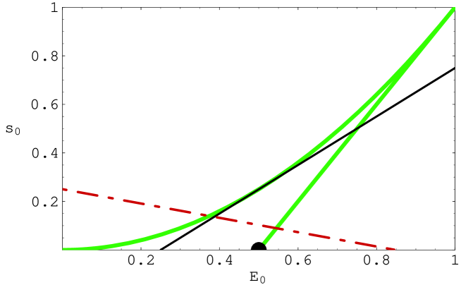
Figure 1: Effect of lepton energy and $M_{X}$ cuts on the $E_{0}-s_{0}$ phase space. See the text for explanations. The cuts employed in the figure are $M_{X}^{\rm cut}=2.4$ GeV and $\xi=0.5$.

It is useful to explain the kinematics with cuts in some detail. The region of integration in the $E_{0}$-$s_{0}$ plane is depicted in Fig. 1: the green (light) solid lines delimit the region of integration without any cut, that is the region between the curves $s_{0}=2E_{0}-1$ and $s_{0}=E_{0}^{2}$. The introduction of a cut in the lepton energy $E_{\ell}^{\rm cut}$ divides this region into three parts that should be treated differently (see e.g. [11]): in the figure these regions are separated by the black (dark) solid line that corresponds to $s_{0}=(1-\xi)(2E_{0}-1+\xi)$. In the first region, between $s_{0}=2E_{0}-1$ and $s_{0}=(1-\xi)(2E_{0}-1+\xi)$ (below the black line), one should use the differential rate calculated with the electron energy cut imposed. There are two regions above the black line, between $s_{0}=(1-\xi)(2E_{0}-1+\xi)$ and $s_{0}=E_{0}^{2}$. In the lower of these two regions, the lepton energy is always above $E_{\ell}^{\rm cut}$, and one should use the differential rate calculated without the cut. Finally, the upper region above the black line is excluded as the lepton energy is always below the cut. Whatever its value, a cut on the lepton energy affects both perturbative and non-perturbative contributions to the moments.

A cut on the hadronic invariant mass $M_{X}^{\rm cut}$ limits the region of integration to the area below the red dash-dotted line, that corresponds to $M_{X}^{2}=(M_{X}^{\rm cut})^{2}$. Increasing the value of $M_{X}^{\rm cut}$, the allowed region of integration expands. For a wide range of values of $M_{X}^{\rm cut}$ and $m_{b}$, as long as the red line does not come close to the $E_{0}$ axis to the left of $E_{0}=1/2$, the introduction of this cut affects only the perturbative corrections to the moments, as it excludes only events characterized by high $s_{0}$ (hard gluon radiation). We limit ourselves to this case and consider only values of $M_{X}^{\rm cut}$ above the lower limit

$$M_{X}^{\rm cut}>\sqrt{M_{B}{\bar{\Lambda}}}\,,$$ (6)

corresponding to the situation in which the cut in ${M_{X}^{2}}$ intersects the $E_{0}$ axis at the value $E_{0}=1/2$ (black dot). Using $m_{b}=4.6$ GeV, for instance, we have $M_{X}^{\rm cut}>1.89$ GeV. In fact, the effect of the $B$ distribution function becomes important within distances of $O(\Lambda_{QCD})$ from the $E_{0}$ axis. As we will see in the next Section, a clean prediction of the moments requires $M_{X}^{\rm cut}$ significantly higher than in the above equation. Table 1 reports our results for the components of ${\cal M}_{(i,j)}$ in the on-shell mass scheme at particular $\xi$ and $M_{X}^{\rm cut}$ values.

i	j	$M_{ij}$	$A^{(1)}_{ij}$	$A^{(2)}_{ij}$
0	0	0.818792	-2.26120	-3.1225
0	1	0.281010	-0.73861	-0.9206
0	2	0.104107	-0.25651	-0.2921
0	3	0.040583	-0.09238	-0.0944
1	0	-0.004709	0.13096	0.2476
1	1	-0.000878	0.05258	0.0979
1	2	0.000058	0.02203	0.0405
2	0	0.002061	0.00496	0.0076
2	1	0.000878	0.00214	0.0032
3	0	0.000115	0.00034	0.0005

Table 1: Various contributions to the building blocks in the on-shell scheme with $E_{\ell}>1$ GeV and $M_{X}<2.5$ GeV. The non-perturbative corrections in $M_{(i,j)}$ are calculated with the default values of the parameters given in Eqs. (7) and $X_{\mu}=28$.

Although we start from on-shell expressions [5, 6], we actually employ the Wilsonian scheme with a hard factorization scale $\mu$, whose optimal value is close to 1 GeV [12]. The Wilson coefficients in this scheme can be determined from the requirement that the observables be $\mu$-independent. The initial condition is that at $\mu\!\to\!0$ one should recover the results in the on-shell scheme. In practice, at low perturbative orders this often reduces to re-expressing the pole-scheme results in terms of the running $\mu$-dependent parameters. In particular, the $\mu$-dependent parameters are the $b$ quark mass $m_{b}(\mu)$, kinetic expectation value $\mu_{\pi}^{2}(\mu)$, and the Darwin expectation value $\rho_{D}^{3}(\mu)$. In the following, our default choice for the non-perturbative parameters evaluated at $\mu=1$ GeV is

$$\ \ \ \ \ \ m_{b}\!=\!4.6\,\mbox{GeV}\ \ \ \mu_{\pi}^{2}\!=\!0.40\,\mbox{GeV}^{2}\ \ \ \mu_{G}^{2}\!=\!0.35\,\mbox{GeV}^{2}$$ (7)

$$\ \ \ \ \rho_{D}^{3}\!=\!0.1\,\mbox{GeV}^{3}\ \ \ \rho_{LS}^{3}\!=\!-0.1\,\mbox{GeV}^{3}\ \ \ \alpha_{s}(m_{b})=0.22\,.$$

The above values for the OPE parameters have been chosen having in mind the central values of the fits to $B\to X_{c}l\nu$ and $B\to X_{s}\gamma$ moments [2] and some additional constraint.

The coefficient function of the Darwin operator that contributes to the $b\!\to\!q\,\ell\nu$ total width at order $1/m_{b}^{3}$ has a logarithmic divergence [8, 9] as $m_{q}\!\to\!0$:

$$C_{D}\simeq-\frac{\Gamma_{0}}{m_{b}^{3}}\left[8\ln\frac{m_{b}^{2}}{m_{q}^{2}}-\frac{77}{6}+{\cal O}\left(\frac{m_{q}^{2}}{m_{b}^{2}}\right)\right].$$ (8)

The singularity originates from the domain of low-momentum final-state quark (i.e., large $q^{2}\!\simeq\!m_{b}^{2}$) and is removed by a one-loop penguin diagram that mixes the four-quark operator $O_{\scriptscriptstyle\rm WA}^{u}=6\bar{b}_{L}^{\alpha}\gamma_{0}b_{L}^{\beta}\,\bar{u}_{L}^{\beta}\gamma^{0}u_{L}^{\alpha}-2\bar{b}_{L}^{\alpha}\vec{\gamma}b_{L}^{\beta}\,\bar{u}_{L}^{\beta}\vec{\gamma}u_{L}^{\alpha}$ (here in its Fierzed form) into the Darwin operator. Let us illustrate how this happens in the total semileptonic width: the lowest order contribution of the Weak Annihilation (WA) operator $O_{\scriptscriptstyle\rm WA}^{u}$ is [16, 17]

$$\delta\Gamma_{\scriptscriptstyle\rm WA}=\Gamma_{0}\ C_{\scriptscriptstyle\rm WA}\ \langle B|O_{\scriptscriptstyle\rm WA}^{u}|B\rangle$$ (9)

where $C_{\scriptscriptstyle\rm WA}=32\pi^{2}/m_{b}^{3}$. In the factorization approximation the matrix element $B_{\scriptscriptstyle\rm WA}\equiv\langle B|O_{\scriptscriptstyle\rm WA}^{u}|B\rangle$ vanishes for $O_{\scriptscriptstyle\rm WA}$ corresponding to zero lepton masses. Including $O(\alpha_{s})$ effects, the above equation becomes

$$\delta\Gamma_{\scriptscriptstyle\rm WA} = \Gamma_{0}\ C_{\scriptscriptstyle\rm WA}\left[\left(1+O(\alpha_{s})\right)B_{\scriptscriptstyle\rm WA}(\mu_{4q})+\frac{\alpha_{s}}{\pi}\,a(\mu_{4q})\langle B|\bar{b}\,t^{a}\,b\sum_{q}\bar{q}\,\gamma_{0}\,t^{a}\,q|B\rangle+...\right]$$ (10)

$$= \Gamma_{0}\left[C_{\scriptscriptstyle\rm WA}\,B_{\scriptscriptstyle\rm WA}(\mu_{4q})-\frac{8\,\rho_{D}^{3}}{m_{b}^{3}}\,\ln\frac{m_{u}^{2}}{\mu_{4q}^{2}}+O(\alpha_{s})\right],$$

where $\mu_{4q}$ is the renormalization scale of the WA operator and $a(\mu_{4q})$ is the contribution of a penguin mixing diagram renormalized in the $\overline{\rm MS}$ scheme. We have used the fact that the Darwin operator is proportional to $g_{s}^{2}\,\bar{b}\,t^{a}\,b\sum_{q}\bar{q}\,\gamma_{0}\,t^{a}q$ by QCD equations of motion, and we have neglected those contributions proportional to the matrix elements of $O_{\scriptscriptstyle\rm WA}^{u}$ and of other operators that come with ${\cal O}(\alpha_{s})$ Wilson coefficients, as they are irrelevant to the present discussion. The constant accompanying the logarithm in Eq. (10) depends on the renormalization scheme; it vanishes in the $\overline{{\rm MS}}$ scheme that we have employed above. We have therefore seen that the inclusion of the WA operator effectively replaces $\ln{m_{b}^{2}}/{m_{u}^{2}}$ in $C_{D}$ by $\ln{m_{b}^{2}}/{\mu_{4q}^{2}}$ plus a constant,

$$C_{D}=-\frac{\Gamma_{0}}{m_{b}^{3}}\left(8\ln\frac{m_{b}^{2}}{\mu_{4q}^{2}}-\frac{77}{6}\right)\,.$$ (11)

Varying the renormalization scale $\mu_{4q}$ adds a piece proportional to $\rho_{D}^{3}$ to the WA expectation value. This contribution is independent of the flavor of the spectator, though, and therefore does not affect the differences between $B^{+}$ and $B^{0}$.

In the following we assume factorization to hold at the scale $\mu_{4q}\!=\!0.8\,\mbox{GeV}$, i.e. $B_{\scriptscriptstyle\rm WA}(0.8\,{\rm GeV})\!\simeq\!0$. A change in $\mu_{4q}$ sets the natural size of the non-factorizable contribution in $B_{\scriptscriptstyle\rm WA}$. To get a crude estimate of how the non-valence (flavor-singlet) non-factorizable component of the expectation value of the WA operator affects the OPE predictions, we may vary $\mu_{4q}$ in the interval $0.4\,\mbox{GeV}\!\mathop{\mbox{\vbox{\hbox{$<$} \vskip-9.0pt\hbox{$\sim$} \vskip-3.0pt}}}\!\mu_{4q}$ $\mathop{\mbox{\vbox{\hbox{$<$} \vskip-9.0pt\hbox{$\sim$} \vskip-3.0pt}}}\!1.7\,\mbox{GeV}$. It is clear, however, that ultimately the size of the WA expectation values in both $B^{0}$ and $B^{+}$ must be determined experimentally. Notice also that, unlike the total width, the parton level moments $M_{(i,j)}$ are not affected by the WA-Darwin mixing for $i,j\neq 0$ (see Appendix A).

In the calculation of the moments we follow [3] closely. In particular, we consider $\bar{\Lambda}={\cal O}(1)$ in the $\Lambda_{QCD}/m_{b}$ expansion and expand in $\Lambda_{QCD}/m_{b}$ and $\alpha_{s}$, neglecting all terms of $O(\alpha_{s}\ \Lambda_{QCD}^{2}/m_{b}^{2})$. This choice makes the hadronic moments sensitive to the choice of $\mu_{4q}$ in Eq. (11). One can parameterize this dependence using $X_{\mu}\equiv 8\ln\frac{m_{b}^{2}}{\mu_{4q}^{2}},$ and vary it in the range $16\leq X_{\mu}\leq 40$, corresponding to the range in $\mu_{4q}$ just discussed, or equivalently use $|B_{\scriptscriptstyle\rm WA}(0.8~{}{\rm GeV})|\leq 0.004\,{\rm GeV}^{3}$. The contribution of the WA operator to the moments can be easily recovered in the following by the replacement $\rho_{D}^{3}\,X_{\mu}\to\rho_{D}^{3}\,X_{\mu}-32\pi^{2}\,B_{\scriptscriptstyle\rm WA}(\mu_{4q})$.

In Table 2 we provide some reference numbers for $U_{1,2,3}$, obtained using $E_{\ell}^{\rm cut}=1$ GeV, $X_{\mu}=28$, and the default values given in Eq. (7) at different values of $M_{X}^{\rm cut}$.

$M_{X}^{\rm cut}$ 2.3 2.5 2.7 3 3.5 $M_{B}$ $U_{1}$ 1.898 1.960 1.997 2.028 2.045 2.047 $U_{2}$ 1.724 1.997 2.062 2.228 2.357 2.377 $U_{3}$ 1.188 1.730 2.338 3.225 4.198 4.416

Table 2: Hadronic moments for $E_{\ell}^{\rm cut}=1~{}\mbox{GeV}$, $B_{\scriptscriptstyle\rm WA}(0.8~{}{\rm GeV})=0$, and the default values given in Eq. (7) at different $M_{X}^{\rm cut}$. The results are in GeV to the appropriate power.

$E_{\ell}^{\rm cut}$ $V$   $B$ $P$ $G$ $D$ $L$   $S$ $Y$ 0 2.179 -3.84 -0.75 0.40 0.84 -0.038 -2.76 10.4 0.6 2.143 -3.80 -0.76 0.42 0.85 -0.035 -2.83 10.6 0.9 2.078 -3.74 -0.80 0.45 0.89 -0.028 -2.96 11.2 1.2 1.973 -3.62 -0.89 0.51 0.96 -0.012 -3.16 12.4 1.5 1.818 -3.40 -1.04 0.60 1.10 0.019 -3.45 14.9

Table 3: Coefficients of the linearized formulas in Eq. (2) for $U_{1}$ at different cuts on the lepton energy without $M_{X}$ cut.

$E_{\ell}^{\rm cut}$ $V$   $B$ $P$ $G$ $D$ $L$   $S$ $Y$ 0 2.832 -0.706 5.11 -0.367 -5.01 -0.04 6.45 -20.8 0.6 2.691 -0.681 4.98 -0.352 -5.07 -0.08 5.89 -21.0 0.9 2.468 -0.452 4.75 -0.329 -5.22 -0.17 5.05 -21.5 1.2 2.173 -0.368 4.39 -0.295 -5.51 -0.30 4.09 -22.9 1.5 1.835 -0.367 3.86 -0.247 -6.04 -0.47 3.33 -26.0

Table 4: Same as in Table 3 but for $U_{2}$.

$E_{\ell}^{\rm cut}$ $V$   $B$ $P$ $G$ $D$ $L$   $S$ $Y$ 0 7.096 1.156 4.72 0.150 20.9 1.3 21.0 35.8 0.6 6.119 1.131 4.62 0.140 20.1 1.2 15.6 35.7 0.9 4.872 0.689 4.55 0.113 18.6 1.1 8.66 35.6 1.2 3.519 0.239 4.52 0.067 16.2 1.0 1.39 35.9 1.5 2.342 -0.104 4.53 0.008 12.8 0.7 -4.30 37.3

Table 5: Same as in Table 3 but for $U_{3}$.

In general, the BLM corrections are almost as relevant and have the same sign as the one-loop perturbative contributions at fixed $\alpha_{s}=0.22$, i.e. they significantly decrease the effective scale of the QCD coupling. It is also convenient to have approximate linearized formulas for a generic moment ${\cal M}$ of the form

$${\cal M}(m_{b},\mu_{\pi}^{2},\mu_{G}^{2},\rho_{D}^{3},\rho_{LS}^{3};\alpha_{s})\mbox{~{}} = \mbox{~{}}V+B\,(m_{b}\!-\!4.6\,\mbox{GeV})+A\,(\alpha_{s}-0.22)\;$$

$$\mbox{~{}}+P\,(\mu_{\pi}^{2}\!-\!0.4\,\mbox{GeV}^{2})+D\,(\rho_{D}^{3}\!-\!0.1\,\mbox{GeV}^{3})\qquad$$

$$\mbox{~{}}+G\,(\mu_{G}^{2}\!-\!0.35\,\mbox{GeV}^{2})+L\,(\rho_{LS}^{3}\!+\!0.1\,\mbox{GeV}^{3})$$

$$\mbox{~{}}+Y\,B_{\scriptscriptstyle\rm WA}(0.8~{}{\rm GeV});$$

The values of $V$ are obtained with the default values of the heavy quark parameters, $B_{\scriptscriptstyle\rm WA}(0.8~{}{\rm GeV})=0$, and are quoted in  GeV to the corresponding power. In Tables 3-5 we report values of the various coefficients with different $E_{\ell}^{\rm cut}$ in the case without an $M_{X}$ cut. For values of $M_{X}^{\rm cut}$ satisfying the bound in Eq. (6) only the perturbative contributions differ from the case without an $M_{X}$ cut. Table 6 therefore shows only the coefficients $V$, $B$, and $S$ for $M_{X}^{\rm cut}=2.5$ GeV and $E_{\ell}^{\rm cut}=0.9$ GeV. The results of our calculation are implemented in a FORTRAN code, available from the authors, that computes hadronic moments in $b\to u$ for arbitrary $E_{\ell}^{\rm cut}$ and for $M_{X}^{\rm cut}$ satisfying Eq. (6).

$V$ $B$ $S$ $U_{1}$ 1.981 -3.56 -3.6 $U_{2}$ 1.939 0.10 1.6 $U_{3}$ 1.743 1.60 -11.7

Table 6: Coefficients of the linearized formulas in Eq. (2) for $U_{1,2,3}$ for $M_{X}^{\rm cut}=2.5$ GeV and $E_{\ell}^{\rm cut}=0.9$ GeV. Only the coefficients that differ from Tables 3-5 are reported.

We can compare the $U_{1}$ values given in Tables 3 and 6 to the preliminary BaBar results of Ref. [1]. With a high $M_{X}$ cut of 5 GeV BaBar find $U_{1}(5~{}{\rm GeV})=2.78\pm 0.82$ GeV², that is in good agreement with our reference value of 2.18 GeV². BaBar also reports a result at low $M_{X}^{\rm cut}=1.86$ GeV which is very close to the lower bound of Eq. (6). In that case their result $U_{1}(1.86~{}{\rm GeV})=1.98\pm 0.20$ GeV² is compatible with the reference value 1.49 GeV² that we obtain at $M_{X}^{\rm cut}=1.9$ GeV, although Fermi motion effects, that shift $U_{1}$ to higher values, have not been included in the calculation (see next Section).

Finally, using our building blocks it is straightforward to study also $q^{2}$ moments. Indeed, replacing $\bar{\Lambda}$ with $-m_{b}$ in the rhs of Eq. (3) one obtains $q^{2}$ and can then calculate the $q^{2}$ moments

$$\langle q^{2n}\rangle=\frac{\int dq^{2}\ q^{2n}\ d\Gamma/dq^{2}}{\int dq^{2}\ d\Gamma/dq^{2}}$$ (13)

in a way similar to the invariant mass moments. Table 7 gives the reference values and the coefficients of the linearized formula of Eq. (2) for the first three moments in the case of $E_{\ell}^{\rm cut}=1.2$ GeV and no cut on $M_{X}$.

  $V$   $B$   $P$   $G$   $D$   $L$   $S$   $10^{3}\,Y$ $\langle q^{2}\rangle$ 7.773 3.058 -0.0193 -0.894 -0.710 -0.186 6.15 -0.084 $\langle q^{4}\rangle$ 81.32 71.35 -0.188 -19.7 -4.26 -4.22 113.6 -2.27 $\langle q^{6}\rangle$ 980.4 1461 -1.417 -381 201 -82.9 1758 -52.2

Table 7: Coefficients of the linearized formulas in Eq. (2) for $\langle q^{2,4,6}\rangle$ with $E_{\ell}^{\rm cut}=1.2$ GeV.

3 Theoretical uncertainty

Let us now consider the various sources of theoretical uncertainty that affect our predictions. First we consider the uncertainty that affects the moments when no upper cut on $M_{X}$ is imposed. If the $E_{\ell}$ cut is not too severe (less than, say, 1.4 GeV), there are four main theoretical systematics:

• uncalculated $O(\alpha_{s}^{2})$ and $O(\alpha_{s}\Lambda^{2,3}_{QCD}/m_{b}^{2,3})$ perturbative contributions to the Wilson coefficients;

• missing $O(1/m_{b}^{4})$ non-perturbative effects;

• the error from the scale in $X_{\mu}$;

• Weak annihilation (WA) contributions.

The first two items are common with the $b\to c$ moments and can be analyzed in a similar way. The last two items, as clarified in the previous Section, are two facets of the same effect, and should not be counted twice. When we include the WA effects as a priori unknown, we use the variation of the scale $\mu_{4q}$ in iii) to estimate the size of its flavor singlet contributions (flavor non-singlet WA effects can be studied from the difference in the moments for charged and neutral $B$). On the other hand, as discussed below, moment measurements allow to place constraints or to detect WA. In this approach fixing $\mu_{4q}$ in $X_{\mu}$ extracts the expectation value of the WA operator normalized (in dimensional regularization) at this point. The remaining uncertainty comes from higher-order corrections to the Wilson coefficients, item i).

In general, we note that $b\to u$ moments are affected by larger theory errors than the $b\to c$ moments. Using the simple recipe given in [3], we estimate the uncertainty related to i) and ii) above by varying $\mu_{\pi}^{2}$, $\mu_{G}^{2}$, and $\alpha_{s}$ by $\pm 20$%, $\rho_{D}^{3}$ and $\rho_{LS}^{3}$ by $\pm$30%, and $m_{b}$ by $\pm$20 MeV in the theoretical predictions in an uncorrelated way. The typical results

$$\delta U_{1}/U_{1}\approx 8\%\ \ \ \delta U_{2}/U_{2}\approx 20\%\ \ \ \delta U_{3}/U_{3}\approx 20\%,$$ (14)

roughly reflect the theory errors due to i) and ii) above, independently of the accuracy with which we know the OPE parameters from [2]. They are driven by the strong sensitivity of $U_{2}$ and $U_{3}$ to $\mu_{\pi}^{2}$ and $\rho_{D}^{3}$.

The uncertainty of Eq. (14) can be estimated in alternative ways. For instance, we can evaluate $U_{1,2,3}$ using a different rearrangement of non-perturbative corrections, namely considering $\bar{\Lambda}$ as an $O(\Lambda_{QCD})$ quantity in the expansion in inverse powers of the $b$ mass. In this case the moments are insensitive to $X_{\mu}$ and to the related error. The results are always within the ranges in Eq. (14). The main step necessary to improve on the above uncertainties is the calculation of perturbative contributions to the Wilson coefficients, of $O(\alpha_{s}^{2})$   and $O(\alpha_{s}/m_{b}^{2,3})$.

For what concerns the value of $B_{\scriptscriptstyle\rm WA}$, as mentioned in the previous section we vary it in the range $|B_{\scriptscriptstyle\rm WA}(0.8~{}{\rm GeV})|\leq 0.004~{}{\rm GeV}^{3}$. This is a rather conservative estimate for the a priori unknown flavor singlet WA contribution, that induces a typical uncertainty of about 2%, 3%, 2% for $U_{1}$, $U_{2}$, $U_{3}$, respectively, although the error can be larger for high $E_{\ell}$ cuts, as it is evident from Tables 3-5.

We recall that WA contributions are concentrated at maximal $q^{2}$, namely at the origin in Fig. 1. In the $(E_{0},s_{0})$ plane the fixed $q^{2}$ contours are straight lines identified by $s_{0}=2E_{0}-1+q^{2}/m_{b}^{2}$. For instance, the r.h.s. boundary of the relevant phase space (the straight green line) corresponds to $q^{2}=0$. WA contributions are therefore characterized by small hadronic invariant mass and can be relevant in the total rate, but are suppressed in the moments of $M_{X}^{2}$.

Turning to the theoretical uncertainty introduced by a cut on $M_{X}$, we have already mentioned in the previous section that low $M_{X}^{\rm cut}$ make the moments sensitive to the $B$ distribution function. A rough but simple way to understand the range of $M_{X}^{\rm cut}$ for which these non-perturbative effects become important is to rewrite Eq. (6) shifting $\bar{\Lambda}$ by the typical width of the distribution function, i.e. $\pm\sqrt{\mu^{2}_{\pi}/3}\approx\pm 0.37$ GeV, to account for the Fermi motion. The result is that distribution function effects become important when $M_{X}^{\rm cut}$ is less than about 2.35 GeV. This result, however, is unlikely to apply to higher moments that are more sensitive to the tail of the distribution function. A detailed estimate would imply a dedicated implementation of the distribution function, which is beyond the scope of the present publication.

A detailed study of similar effects in the photon energy moments of $B\!\to\!X_{s}+\gamma$ [4] showed that if the Wilsonian-type OPE with the hard cutoff at the scale around $1\,\mbox{GeV}$ is used, the inclusion of perturbative corrections affects only marginally the bias induced by Fermi motion. At the same time, the estimates are sensitive to the $1/m_{b}$ corrections that decrease the variance of the light-cone distribution with respect to the heavy quark limit. Based on that experience, we have estimated the Fermi motion effects introduced by the $M_{X}$ cut in the $b\!\to\!u\,\ell\nu$ moments by smearing the tree-level differential rate with an exponential distribution function (see eq.(13) of Ref. [4]) characterized by the low value $\mu_{\pi}^{2}\!\approx\!0.36\,\mbox{GeV}^{2}$, to approximately account for the $1/m_{b}$ contributions to the second moment of the distribution function. Since the calculation of the hadronic moments is sensitive to the tail of the distribution, this estimate depends critically on the functional form adopted. In this respect, our choice of the exponential form leads to more conservative estimates than, say, with a Gaussian ansatz. Comparing the moments at $M_{X}^{\rm cut}=M_{B}$ to those at various $M_{X}^{\rm cut}$, we find that the Fermi motion may alter $U_{1}$ by $\sim 6\%$ at $M_{X}^{\rm cut}=2.5$ GeV and by $\sim 3\%$ at $M_{X}^{\rm cut}=2.7$ GeV. The higher moments are of course more sensitive: $U_{2}$ may vary by $30\%$ at $M_{X}^{\rm cut}=2.5$ GeV and by $\sim 20\%$ at $M_{X}^{\rm cut}=2.7$ GeV, while $U_{3}$ is dramatically affected – $O(1)$ effects – below $M_{X}^{\rm cut}=$2.7 GeV; the Fermi motion effects might become comparable to the other uncertainties only above $M_{X}^{\rm cut}=3$ GeV. Such high $M_{X}^{\rm cut}$ values are certainly challenging for present experiments, but preliminary studies indicate the possibility of measuring the moments with interesting accuracy even for $M_{X}^{\rm cut}$ well above the charm threshold [15].

Finally, let us discuss the uncertainty in the evaluation of the $q^{2}$ moments. We have already mentioned that these moments are very sensitive to the WA contributions, and therefore can be used to detect or place constraints on them. The flavor non-singlet WA contributions can be studied by comparing the $q^{2}$ moments (or other decay characteristics) measured in charged and neutral $B$ decays separately [16]. For precision studies it is important to control the flavor singlet component of WA as well. They can be constrained by comparing the OPE predictions with data. In that respect, we need to consider only the uncertainties listed under i) and ii); regarding them in the same way as for the hadronic moments, the results are

$$\delta\langle q^{2}\rangle/\langle q^{2}\rangle\approx 3\%\ \ \ \delta\langle q^{4}\rangle/\langle q^{4}\rangle\approx 6\%\ \ \ \delta\langle q^{6}\rangle/\langle q^{6}\rangle\approx 9\%$$ (15)

and are dominated by perturbative effects. As mentioned in the previous section, the sensitivity of the various moments to the WA contributions can be understood from their $X_{\mu}$ dependence: varying $B_{\scriptscriptstyle\rm WA}(0.8~{}{\rm GeV})$ in the usual range and using the linearized formula of Eq. (2), we obtain a shift of approximately $4\%$, 11%, 21%, for the first three $q^{2}$ moments, respectively. Since we only consider $q^{2}$ moments without cuts on $M_{X}$, we do not have Fermi motion effects.

4 Summary

We have calculated the first three moments of the hadronic invariant mass distribution in charmless semileptonic decays in a Wilsonian scheme characterized by a hard cutoff $\mu\sim 1$ GeV. Our calculation includes all known perturbative and non-perturbative effects, through $O(\alpha_{s}^{2}\beta_{0})$ and $O(1/m_{b}^{3})$ and is implemented in a FORTRAN code available from the authors. As required by the present experimental situation, we have considered cuts on the lepton energy and on the invariant hadronic mass and have obtained approximate formulas that summarize the dependence of the moments on the OPE parameters.

The theoretical uncertainty of our OPE predictions ranges from 5% to 30%, but an upper cut on $M_{X}$ introduces a dependence on the Fermi motion of the $b$ quark in the meson. While we have performed a first estimate of these effects, the subject requires a more detailed investigation that we postpone to a future publication. Moreover, as the constraints on the shape of the distribution function are likely to improve in the future, our estimates of the Fermi motion effects should not be considered as an irreducible uncertainty. Conversely, the $M_{X}$ spectrum and its truncated moments can themselves be used to constrain the distribution function, especially in the tail that is not accessible in radiative decays.

We find that the bias introduced by the distribution function is not important for the first hadronic moment, if the $M_{X}$ cut is placed above 2.5–2.7 GeV. In that case its theoretical uncertainty is in the 10% range. The prediction for the second central moment, $U_{2}$, is subject to a 20% uncertainty even without a cut on $M_{X}$. For cuts on $M_{X}$ higher than $\sim 2.7~{}$GeV, the Fermi motion uncertainty on $U_{2}$ may be as high as 20%. Finally, the third central moment, $U_{3}$, is very sensitive to Fermi motion and can be predicted with a meaningful accuracy ($\sim 20\%$) only if the cut on $M_{X}$ is higher than $\sim 3.2~{}$GeV.

We have also considered $q^{2}$ moments which could soon be measurable and are particularly sensitive to WA. They can be predicted with good accuracy in the local OPE, provided the cut on the lepton energy is sufficiently low, $E_{\ell}^{\rm cut}\mathop{\mbox{\vbox{\hbox{$<$} \vskip-9.0pt\hbox{$\sim$} \vskip-3.0pt}}}1.5$ GeV. We have shown how it is possible to constrain both the flavor singlet and the flavor non-singlet WA contributions. In view of their potential interest, they should therefore be measured with $E_{\ell}^{\rm cut}$ as low as possible.

Appendix A: non-perturbative corrections

Here we give explicit expressions for the lowest order and OPE contributions to $M_{ij}$, in the case of a lower cut on the charged lepton energy. They agree with Ref. [18] for $\xi=0$.

$$M_{(0,0)} = 1+\xi^{4}-2\xi^{3}-\frac{1}{6}\frac{\mu^{2}_{G}}{m_{b}^{2}}\left(5\xi^{4}+8\xi^{3}+9\right)+\frac{1}{6}\frac{\mu^{2}_{\pi}}{m_{b}^{2}}\left(5\xi^{4}-3\right)+\frac{\rho^{3}_{LS}}{m_{b}^{3}}\frac{\xi^{4}+9}{6}$$

$$+\frac{\rho^{3}_{D}}{m_{b}^{3}}\left(\frac{\xi^{4}}{6}+\frac{8\xi^{3}}{3}-4\xi^{2}-8\xi-8\ln(1-\xi)+\frac{77}{6}-X_{\mu}\right)$$

$$M_{(0,1)} = \frac{-2\xi^{5}+15\xi^{4}-20\xi^{3}+7}{20}+\frac{1}{12}\frac{\mu^{2}_{G}}{m_{b}^{2}}\left(\xi^{2}-4\xi-6\right)\xi^{3}-\frac{1}{12}\frac{\mu^{2}_{\pi}}{m_{b}^{2}}\left(\xi^{5}-6\xi^{4}-2\xi^{3}+6\right)$$

$$+\frac{1}{60}\frac{\rho^{3}_{LS}}{m_{b}^{3}}\left(-\xi^{5}+10\xi^{4}+30\xi^{3}+6\right)+\frac{1}{60}\frac{\rho^{3}_{D}}{m_{b}^{3}}\left(-\xi^{5}+10\xi^{4}+90\xi^{3}-134\right)$$

$$M_{(0,2)} = \frac{1}{60}\left(\xi^{6}-9\xi^{5}+30\xi^{4}-30\xi^{3}+8\right)+\frac{1}{360}\frac{\mu^{2}_{G}}{m_{b}^{2}}\left(-5\xi^{6}+24\xi^{5}-60\xi^{4}-60\xi^{3}+26\right)$$

$$+\frac{1}{360}\frac{\mu^{2}_{\pi}}{m_{b}^{2}}\left(5\xi^{6}-36\xi^{5}+120\xi^{4}-86\right)+\frac{1}{360}\frac{\rho^{3}_{D}}{m_{b}^{3}}\left(\xi^{6}-12\xi^{5}+30\xi^{4}+120\xi^{3}-48\right)$$

$$+\frac{1}{360}\frac{\rho^{3}_{LS}}{m_{b}^{3}}\left(\xi^{6}-12\xi^{5}+30\xi^{4}+120\xi^{3}-28\right)$$

$$M_{(0,3)} = \frac{-2\xi^{7}+21\xi^{6}-84\xi^{5}+175\xi^{4}-140\xi^{3}+30}{560}$$

$$+\frac{\mu^{2}_{G}}{m_{b}^{2}}\frac{\left(5\xi^{7}-28\xi^{6}+84\xi^{5}-175\xi^{4}-70\xi^{3}+72\right)}{1680}$$

$$+\frac{\mu^{2}_{\pi}}{m_{b}^{2}}\frac{\left(-5\xi^{7}+42\xi^{6}-168\xi^{5}+490\xi^{4}-210\xi^{3}-156\right)}{1680}$$

$$+\frac{\rho^{3}_{LS}}{m_{b}^{3}}\frac{\left(-\xi^{7}+14\xi^{6}-42\xi^{5}+140\xi^{4}+210\xi^{3}-104\right)}{1680}$$

$$+\frac{\rho^{3}_{D}}{m_{b}^{3}}\frac{\left(-\xi^{7}+14\xi^{6}-42\xi^{5}+420\xi^{4}-70\xi^{3}-48\right)}{1680}$$

$$M_{(1,0)} = \frac{1}{12}\frac{\mu^{2}_{G}}{m_{b}^{2}}\left(-2\xi^{5}-5\xi^{4}+4\xi^{3}+3\right)+\frac{1}{60}\frac{\mu^{2}_{\pi}}{m_{b}^{2}}\left(14\xi^{5}-15\xi^{4}+20\xi^{3}-39\right)$$

$$+\frac{1}{60}\frac{\rho^{3}_{LS}}{m_{b}^{3}}\left(-2\xi^{5}-35\xi^{4}+60\xi^{3}-3\right)+\frac{1}{60}\frac{\rho^{3}_{D}}{m_{b}^{3}}\left(-2\xi^{5}+65\xi^{4}-140\xi^{3}+177\right)$$

$$M_{(2,0)} = \frac{1}{45}\frac{\mu^{2}_{\pi}}{m_{b}^{2}}\left(\xi^{6}-9\xi^{5}+30\xi^{4}-30\xi^{3}+8\right)+\frac{1}{45}\frac{\rho^{3}_{D}}{m_{b}^{3}}\left(-2\xi^{6}+9\xi^{5}-15\xi^{4}+30\xi^{3}-31\right)$$

$$+\frac{1}{45}\frac{\rho^{3}_{LS}}{m_{b}^{3}}\left(-\xi^{6}-15\xi^{5}+45\xi^{4}-30\xi^{3}+1\right)$$

$$M_{(3,0)} = \frac{1}{210}\frac{\rho^{3}_{D}}{m_{b}^{3}}\left(-2\xi^{7}+21\xi^{6}-84\xi^{5}+175\xi^{4}-140\xi^{3}+30\right)$$

$$M_{(1,1)} = \frac{1}{180}\frac{\mu^{2}_{G}}{m_{b}^{2}}\left(5\xi^{6}-3\xi^{5}-45\xi^{4}+30\xi^{3}+13\right)+\frac{1}{180}\frac{\mu^{2}_{\pi}}{m_{b}^{2}}\left(-7\xi^{6}+27\xi^{5}+15\xi^{4}-30\xi^{3}-23\right)$$

$$+\frac{1}{180}\frac{\rho^{3}_{D}}{m_{b}^{3}}\left(\xi^{6}-21\xi^{5}+165\xi^{4}-150\xi^{3}+71\right)+\frac{1}{180}\frac{\rho^{3}_{LS}}{m_{b}^{3}}\left(\xi^{6}+15\xi^{5}-15\xi^{4}+30\xi^{3}-13\right)$$

$$M_{(2,1)} = \frac{1}{420}\frac{\mu^{2}_{\pi}}{m_{b}^{2}}\left(-2\xi^{7}+21\xi^{6}-84\xi^{5}+175\xi^{4}-140\xi^{3}+30\right)$$

$$+\frac{1}{420}\frac{\rho^{3}_{D}}{m_{b}^{3}}\left(4\xi^{7}-21\xi^{6}+28\xi^{5}+35\xi^{4}-74\right)$$

$$+\frac{\rho^{3}_{LS}}{m_{b}^{3}}\frac{\left(6\xi^{7}+77\xi^{6}-420\xi^{5}+735\xi^{4}-420\xi^{3}+22\right)}{1260}$$

$$M_{(1,2)} = \frac{\mu^{2}_{G}}{m_{b}^{2}}\frac{\left(-10\xi^{7}+21\xi^{6}+56\xi^{5}-245\xi^{4}+140\xi^{3}+38\right)}{1680}$$

$$+\frac{1}{240}\frac{\mu^{2}_{\pi}}{m_{b}^{2}}\left(2\xi^{7}-11\xi^{6}+8\xi^{5}+55\xi^{4}-60\xi^{3}-2\right)$$

$$+\frac{\rho^{3}_{LS}}{m_{b}^{3}}\frac{\left(-6\xi^{7}-91\xi^{6}+84\xi^{5}+735\xi^{4}-420\xi^{3}-134\right)}{5040}$$

$$+\frac{\rho^{3}_{D}}{m_{b}^{3}}\frac{\left(-2\xi^{7}+35\xi^{6}-364\xi^{5}+1155\xi^{4}-700\xi^{3}+30\right)}{1680}$$

Appendix B: ${\cal O}(\alpha_{s})$ corrections to the moments

We report here analytic formulas for the ${\cal O}(\alpha_{s})$ perturbative corrections to the building blocks $M_{ij}$ defined in Eq. (2) when a lower cut on the lepton energy is applied. The expressions are valid in the on-shell scheme for the $b$ quark mass and they agree with Ref. [18] for $\xi=0$. We employ the short-hand $L_{\xi}=\ln(1-\xi)$.

$$A^{(1)}_{(0,0)} = -\frac{4}{9}\pi^{2}\xi^{4}+\frac{47\xi^{4}}{18}+\frac{8\pi^{2}\xi^{3}}{9}-\frac{59\xi^{3}}{9}+\frac{50\xi^{2}}{9}-\frac{52\xi}{9}-\frac{2\pi^{2}}{3}+\frac{25}{6}+\frac{4\xi^{3}}{3}\left(2-\xi\right)\mbox{Li}_{2}(\xi)$$

$$+L_{\xi}\left(-\frac{8\xi^{4}}{9}+\frac{32\xi^{3}}{9}-\frac{14\xi^{2}}{3}+\frac{70\xi}{9}-\frac{52}{9}\right)+L_{\xi}^{2}\left(-\frac{2\xi^{4}}{3}+\frac{4\xi^{3}}{3}-\frac{2}{3}\right)$$

$$A^{(1)}_{(0,1)} = \frac{2\pi^{2}\xi^{5}}{45}-\frac{103\xi^{5}}{450}-\frac{\pi^{2}\xi^{4}}{3}+\frac{7\xi^{4}}{4}+\frac{4\pi^{2}\xi^{3}}{9}-\frac{1213\xi^{3}}{360}+\frac{191\xi^{2}}{72}-\frac{421\xi}{180}$$

$$+L_{\xi}\left(\frac{4\xi^{5}}{45}-\frac{91\xi^{4}}{180}+\frac{91\xi^{3}}{90}-\frac{83\xi^{2}}{45}+\frac{323\xi}{90}-\frac{421}{180}\right)$$

$$+L_{\xi}^{2}\left(\frac{\xi^{5}}{15}-\frac{\xi^{4}}{2}+\frac{2\xi^{3}}{3}-\frac{7}{30}\right)+\mbox{Li}_{2}(\xi)\left(\frac{2\xi^{5}}{15}-\xi^{4}+\frac{4\xi^{3}}{3}\right)-\frac{7\pi^{2}}{30}+\frac{1381}{900}$$

$$A^{(1)}_{(0,2)} = -\frac{1}{135}\pi^{2}\xi^{6}+\frac{329\xi^{6}}{8100}+\frac{\pi^{2}\xi^{5}}{15}-\frac{497\xi^{5}}{1350}-\frac{2\pi^{2}\xi^{4}}{9}$$

$$+\frac{3757\xi^{4}}{2700}+\frac{2\pi^{2}\xi^{3}}{9}-\frac{71057\xi^{3}}{32400}+\frac{1121\xi^{2}}{675}-\frac{782\xi}{675}-\frac{4\pi^{2}}{45}+\frac{2257}{3600}$$

$$+L_{\xi}\left(-\frac{2\xi^{6}}{135}+\frac{19\xi^{5}}{180}-\frac{37\xi^{4}}{180}+\frac{73\xi^{3}}{180}-\frac{77\xi^{2}}{60}+\frac{484\xi}{225}-\frac{782}{675}\right)$$

$$+L_{\xi}^{2}\left(-\frac{\xi^{6}}{90}+\frac{\xi^{5}}{10}-\frac{\xi^{4}}{3}+\frac{\xi^{3}}{3}-\frac{4}{45}\right)+\mbox{Li}_{2}(\xi)\left(-\frac{\xi^{6}}{45}+\frac{\xi^{5}}{5}-\frac{2\xi^{4}}{3}+\frac{2\xi^{3}}{3}\right)$$

$$A^{(1)}_{(0,3)} = \frac{\pi^{2}\xi^{7}}{630}-\frac{5231\xi^{7}}{529200}-\frac{\pi^{2}\xi^{6}}{60}+\frac{5237\xi^{6}}{50400}+\frac{\pi^{2}\xi^{5}}{15}-\frac{24163\xi^{5}}{50400}-\frac{5\pi^{2}\xi^{4}}{36}+\frac{123257\xi^{4}}{100800}$$

$$+\frac{\pi^{2}\xi^{3}}{9}-\frac{49307\xi^{3}}{30240}+\frac{116689\xi^{2}}{100800}-\frac{32143\xi}{50400}-\frac{\pi^{2}}{28}+\frac{289223}{1058400}$$

$$+L_{\xi}\left(\frac{\xi^{7}}{315}-\frac{137\xi^{6}}{5040}+\frac{99\xi^{5}}{1400}-\frac{361\xi^{4}}{3360}+\frac{205\xi^{3}}{504}-\frac{2413\xi^{2}}{2100}+\frac{9077\xi}{6300}-\frac{32143}{50400}\right)$$

$$+L_{\xi}^{2}\left(\frac{\xi^{7}}{420}-\frac{\xi^{6}}{40}+\frac{\xi^{5}}{10}-\frac{5\xi^{4}}{24}+\frac{\xi^{3}}{6}-\frac{1}{28}\right)+\mbox{Li}_{2}(\xi)\left(\frac{\xi^{7}}{210}-\frac{\xi^{6}}{20}+\frac{\xi^{5}}{5}-\frac{5\xi^{4}}{12}+\frac{\xi^{3}}{3}\right)$$

$$A^{(1)}_{(1,0)} = \frac{\xi^{5}}{50}-\frac{7\xi^{4}}{45}-\frac{37\xi^{3}}{90}+\frac{127\xi^{2}}{90}-\frac{16\xi}{15}+\frac{91}{450}+L_{\xi}\left(-\frac{\xi^{5}}{10}+\frac{8\xi^{4}}{9}-\frac{5\xi^{3}}{3}+\frac{35\xi}{18}-\frac{16}{15}\right)$$

$$A^{(1)}_{(2,0)} = \frac{31\xi^{6}}{4050}-\frac{11\xi^{5}}{135}+\frac{1207\xi^{4}}{2700}-\frac{1912\xi^{3}}{2025}+\frac{574\xi^{2}}{675}-\frac{199\xi}{675}+\frac{5}{324}$$

$$+L_{\xi}\left(\frac{13\xi^{6}}{1350}-\frac{13\xi^{5}}{150}+\frac{4\xi^{4}}{45}+\frac{61\xi^{3}}{135}-\frac{7\xi^{2}}{6}+\frac{449\xi}{450}-\frac{199}{675}\right)$$

$$A^{(1)}_{(1,1)} = \frac{7\xi^{6}}{900}-\frac{31\xi^{5}}{450}+\frac{301\xi^{4}}{900}-\frac{202\xi^{3}}{225}+\frac{1007\xi^{2}}{900}-\frac{263\xi}{450}+\frac{9}{100}$$

$$+L_{\xi}\left(\frac{\xi^{6}}{60}-\frac{77\xi^{5}}{450}+\frac{5\xi^{4}}{9}-\frac{19\xi^{3}}{45}-\frac{29\xi^{2}}{36}+\frac{127\xi}{90}-\frac{263}{450}\right)$$

$$A^{(1)}_{(2,1)} = -\frac{937\xi^{7}}{264600}+\frac{2791\xi^{6}}{75600}-\frac{103\xi^{5}}{504}+\frac{22087\xi^{4}}{37800}-\frac{32167\xi^{3}}{37800}+\frac{1027\xi^{2}}{1680}-\frac{2291\xi}{12600}+\frac{1081}{132300}$$

$$+L_{\xi}\left(-\frac{13\xi^{7}}{6300}+\frac{41\xi^{6}}{1800}-\frac{23\xi^{5}}{450}-\frac{43\xi^{4}}{360}+\frac{13\xi^{3}}{20}-\frac{1837\xi^{2}}{1800}+\frac{158\xi}{225}-\frac{2291}{12600}\right)$$

$$A^{(1)}_{(1,2)} = -\frac{659\xi^{7}}{176400}+\frac{367\xi^{6}}{9450}-\frac{143\xi^{5}}{700}+\frac{14873\xi^{4}}{25200}-\frac{14521\xi^{3}}{15120}+\frac{1759\xi^{2}}{2100}-\frac{536\xi}{1575}+\frac{7421}{176400}$$

$$+L_{\xi}\left(-\frac{\xi^{7}}{280}+\frac{19\xi^{6}}{450}-\frac{37\xi^{5}}{225}+\frac{2\xi^{4}}{9}+\frac{9\xi^{3}}{40}-\frac{89\xi^{2}}{90}+\frac{907\xi}{900}-\frac{536}{1575}\right)$$

$$A^{(1)}_{(3,0)} = -\frac{311\xi^{7}}{66150}+\frac{11\xi^{6}}{252}-\frac{689\xi^{5}}{3150}+\frac{10117\xi^{4}}{18900}-\frac{6259\xi^{3}}{9450}+\frac{2561\xi^{2}}{6300}-\frac{323\xi}{3150}+\frac{377}{132300}$$

$$+L_{\xi}\left(-\frac{\xi^{7}}{525}+\frac{\xi^{6}}{50}-\frac{\xi^{5}}{75}-\frac{19\xi^{4}}{90}+\frac{29\xi^{3}}{45}-\frac{119\xi^{2}}{150}+\frac{103\xi}{225}-\frac{323}{3150}\right)$$

References

- [1] B. Aubert et al. [BABAR Coll.], arXiv:hep-ex/0408068.
- [2] B. Aubert et al. [BABAR Coll.], Phys. Rev. Lett. 93 (2004) 011803 [hep-ex/0404017]; C. W. Bauer et al., Phys. Rev. D 70 (2004) 094017 [hep-ph/0408002] v3; O. Buchmueller and H. Flaecher, contribution to the CKM-2005 Workshop, San Diego, march 2005, http://ckm2005.ucsd.edu/WG/WG2/thu3/henning-WG2-S2.pdf and arXiv:hep-ph/0507253.
- [3] P. Gambino and N. Uraltsev, Eur. Phys. J. C 34 (2004) 181 [arXiv:hep-ph/0401063].
- [4] D. Benson, I. I. Bigi and N. Uraltsev, Nucl. Phys. B 710 (2005) 371 [arXiv:hep-ph/0410080].
- [5] V. Aquila, P. Gambino, G. Ridolfi and N. Uraltsev, arXiv:hep-ph/0503083.
- [6] F. De Fazio and M. Neubert, JHEP 9906, 017 (1999) [arXiv:hep-ph/9905351].
- [7] I. Bigi, N. Uraltsev and A. Vainshtein, Phys. Lett. B293 (1992) 430 and Phys. Rev. Lett. 71 (1993) 496; B. Blok, L. Koyrakh, M. Shifman and A. Vainshtein, Phys. Rev. D49 (1994) 3356; A. V. Manohar and M. B. Wise, Phys. Rev. D 49 (1994) 1310.
- [8] M. Gremm and A. Kapustin, Phys. Rev. D55 (1997) 6924.
- [9] B. Blok, R. D. Dikeman and M. A. Shifman, Phys. Rev. D 51 (1995) 6167 [arXiv:hep-ph/9410293].
- [10] T. van Ritbergen, Phys. Lett. B 454 (1999) 353 [arXiv:hep-ph/9903226]; M. E. Luke, M. J. Savage and M. B. Wise, Phys. Lett. B 343 (1995) 329 [arXiv:hep-ph/9409287]; P. Ball, M. Beneke and V. M. Braun, Phys. Rev. D 52 (1995) 3929 [arXiv:hep-ph/9503492].
- [11] A. F. Falk and M. E. Luke, Phys. Rev. D 57 (1998) 424 [arXiv:hep-ph/9708327].
- [12] I. I. Y. Bigi, M. A. Shifman, N. Uraltsev and A. I. Vainshtein, Phys. Rev. D 56 (1997) 4017 [arXiv:hep-ph/9704245] and Phys. Rev. D 52 (1995) 196 [arXiv:hep-ph/9405410].
- [13] D. Benson, I. I. Bigi, T. Mannel and N. Uraltsev, Nucl. Phys. B 665 (2003) 367 [arXiv:hep-ph/0302262].
- [14] A. Czarnecki and K. Melnikov, Phys. Rev. Lett. 88 (2002) 131801 [arXiv:hep-ph/0112264].
-
[15]
M. Battaglia, talk at BaBar workshop, SLAC, december 2004;
K. Tackmann, talk at CKM 2005, San Diego, march 2005, http://ckm2005.ucsd.edu/WG/WG2/fri2/tackman1-WG2-S4.pdf. - [16] I. I. Y. Bigi and N. G. Uraltsev, Nucl. Phys. B 423 (1994) 33 [arXiv:hep-ph/9310285].
- [17] M. B. Voloshin, Phys. Lett. B 515 (2001) 74 [arXiv:hep-ph/0106040].
- [18] A. F. Falk, M. E. Luke and M. J. Savage, Phys. Rev. D 53 (1996) 2491 [arXiv:hep-ph/9507284].