KamLAND neutrino spectra in energy and time:
Indications for reactor power variations
and constraints on the georeactor

Abstract

The Kamioka Liquid scintillator Anti-Neutrino Detector (KamLAND) is sensitive to the neutrino event spectrum from (mainly Japanese) nuclear reactors in both the energy domain and the time domain. While the energy spectrum of KamLAND events allows the determination of the neutrino oscillation parameters, the time spectrum can be used to monitor known and unknown neutrino sources. By using available monthly-binned data on event-by-event energies in KamLAND and on reactor powers in Japan, we perform a likelihood analysis of the neutrino event spectra in energy and time, and find significant indications in favor of time variations of the known reactor sources, as compared with the hypothetical case of constant reactor neutrino flux. We also find that the KamLAND data place interesting upper limits on the power of a speculative nuclear reactor operating in the Earth’s core (the so-called georeactor); such limits are strengthened by including solar neutrino constraints on the neutrino mass and mixing parameters. Our results corroborate the standard interpretation of the KamLAND signal as due to oscillating neutrinos from known reactor sources.

I Introduction

The Kamioka Liquid scintillator Anti-Neutrino Detector (KamLAND) KamL ; Grat is sensitive to oscillations Pont ; Maki of reactor neutrinos Bemp over long baselines ($\langle L\rangle\sim 180$ km). The neutrino disappearance effect observed in KamLAND Kam1 ; Kam2 ; Kam3 provides an independent confirmation of the matter-enhanced adiabatic solution Adia ; Matt to the solar neutrino problem Bahc ; Home ; SAGE ; GALL ; GNOx ; SKso ; SNO1 ; SNO2 at large mixing angle (LMA), with best-fit oscillation parameters $(\delta m^{2},\sin^{2}\theta_{12})\simeq(7.9\times 10^{-5}\mathrm{\ eV}^{2},0.31)$ Kam2 ; SNO2 in standard notation PDG4 . In addition, the current KamLAND statistics and energy resolution allow to track the oscillatory pattern of reactor neutrinos in the energy domain for about half a period Kam2 .

Being a real-time detector, KamLAND can also track neutrino source variations in the time domain. In particular, significant power variations of some Japanese reactors occurred during data taking Grat , leading to expected variations in the KamLAND neutrino event rate Kam2 . The KamLAND sensitivity to time variations was estimated to reach potentially the $\sim 2.3\sigma$ level through the unbinned test proposed in Unbi , where only time information (and no energy information) was considered.

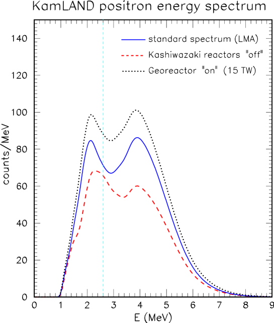
Figure 1: KamLAND absolute spectrum (without backgrounds) as a function of prompt energy. Solid curve: standard spectrum for best-fit LMA parameters. Dashed curve: spectrum with no contributions from the Kashiwazaki reactor power plant. Dotted curve: spectrum with additional contribution from a 15 TW georeactor. The vertical line indicates the analysis threshold (2.6 MeV).

There is also, in principle, an interesting interplay between time and energy information in KamLAND. In the presence of neutrino oscillations, time variations of reactors placed at different distances produce time variations of the energy spectrum. Figure 1 shows, e.g., that by “switching off” one of the most powerful nuclear reactor plants in Japan (namely, Kashiwazaki) one gets not only an overall decrease of the spectrum normalization, but also a slight displacement of the dip in the oscillatory pattern. In the same figure, one can also see the effect of a hypothetical reactor at the center of the Earth (the so-called georeactor Geo1 ), which would increase the KamLAND spectrum by a factor which is constant in time but, in general, not uniform in energy. A joint analysis in the energy and time domain would be appropriate to study such effects.

So far, the KamLAND collaboration has published only one test of the time-variation hypothesis, which makes use of a relatively coarse time binning and of no energy information. The results are shown in the first figure of Ref. Kam2 , where the observed event rates—grouped in five data points—are plotted against the unoscillated reactor neutrino flux, and a positive (expected) correlation is seen to emerge. However, the statistical difference between the two extreme cases in this test (with and without time variations of the neutrino flux) is only $\Delta\chi^{2}=3.3$ Grat , i.e., smaller than $2\sigma$. At a similar significance level, the extrapolation to “zero reactor power” is consistent with the known background, but yields poor constraints on possible unidentified sources such as the georeactor Kam2 .

The power of a time-variation test—as the one described in Kam2 —can be improved by exploiting additional information. For instance, daily data about individual Japanese reactor operations are available to the KamLAND collaboration, through an agreement with the power companies Ku03 . In principle, these data allow one to perform detailed likelihood analyses of the event spectra not only in the energy domain (as those, e.g., in Kam1 ; Kam2 ; SKso ; SNO2 ; Fo03 ; Ia03 ; Schw ; Ricc ; Smir ; Ba04 ; Va04 ; Al04 ; Ma05 ; Go05 ; St05 ) but also in the time domain, thus providing statistically more powerful tests of reactor power variations and of the georeactor hypothesis. Unfortunately, daily reactor data are classified Ku03 .

Recently, monthly-binned data from nuclear reactors and from KamLAND have become publicly available. In particular, average Japanese reactor powers in each calendar month can be found at JAIF . The sequence of published KamLAND events Kam3 in monthly bins, together with the corresponding detector livetime (in seconds), can be found in File . The availability of these data has prompted us to extend the likelihood analysis of KamLAND data in the energy domain (event by event) Kam1 ; Kam2 ; Schw so as to include the time domain (monthly binned). We find that the joint maximum-likelihood analysis in energy and time can provide a significant ($\sim 3\sigma$) indication in favor of time variations of reactor powers, as compared with the case of average constant powers. In addition, we find no indication in favor of a georeactor contribution, and we set upper bounds on its power. In both cases, we discuss the role of additional solar neutrino constraints on $(\delta m^{2},\sin^{2}\theta_{12})$. Our results corroborate the standard interpretation of the KamLAND signal as due to flavor oscillations of neutrinos coming from known reactor sources.

The structure of this paper is as follows. In Sec. II we reproduce, as a preliminary but relevant check, the official KamLAND unbinned likelihood analysis in the energy domain Kam2 ; Kam3 . In sec. III we extend the analysis to the (monthly binned) time domain, and show that significant indications in favor of reactor time variations emerge from the data. In Sec. IV we discuss the effects of a hypothetical georeactor, and set upper bounds on its power. We summarize our results in Sec. V.

A final remark is in order. Our results, although encouraging, cannot—and must not—be taken as a substitute for future, official KamLAND tests of hypotheses about the reactor sources. In fact, as described in the following, our approach involves some unavoidable approximations, which could be easily removed by the KamLAND collaboration—possibly leading to somewhat different results. Nevertheless, we think that our approximate analysis in the energy-time domain may represent an interesting step beyond previous KamLAND data analyses, where the time information is absent.

II Likelihood analysis in energy

The KamLAND experiment has collected so far $N_{\mathrm{obs}}=258$ events in a fiducial mass $M=543.7$ tons, during a total livetime $\Delta t=515.1$ days Kam2 :

$$M\cdot\Delta t=0.766\mathrm{\ kTy}.$$ (1)

Details on the likelihood analysis of the energy spectrum of such events are available at Kam3 . In this Section we reproduce the results of the official KamLAND likelihood analysis in energy Kam2 , before generalizing it to the time domain in Sec. III.

In general, the KamLAND unbinned likelihood function $\mathcal{L}$ can be written as Kam1 ; Kam2 ; Schw :

$$\mathcal{L}=\mathcal{L}_{\mathrm{rate}}\times\mathcal{L}_{\mathrm{shape}}\times\mathcal{L}_{\mathrm{syst}}\ ,$$ (2)

where the three factors embed information on the total event rate, on the spectrum shape, and on systematic uncertainties. The evaluation of $\mathcal{L}$ implies a detailed calculation of the absolute spectrum of events (signal plus background), whose ingredients are briefly described below.

II.1 Reactor input

The reactor signal in KamLAND is essentially generated by 20 nuclear reactor power plants (16 in Japan and 4 in Korea) located at different distances $L_{j}$ and characterized by different thermal powers $P_{j}^{\mathrm{th}}$ Grat . For Japanese reactors ($j=1,\dots,16$), the sequence of monthly-averaged thermal powers $P_{jm}^{\mathrm{th}}$ (where $m$ is a monthly index) can be recovered from the corresponding sequence of average electric powers $P_{jm}^{\mathrm{el}}$ available in JAIF , by using the relation $P^{\mathrm{th}}\simeq 3\,P^{\mathrm{el}}$ Prop . The time interval of interest for the current KamLAND analysis spans $m=1,\dots,23$ months, from March 2002 to January 2004 included Kam2 ; File . In each month, the KamLAND detector livetime $\Delta t_{m}$ (with $\sum_{m}\Delta t_{m}=\Delta t$) is given in File . The average thermal power of the $j$-th Japanese reactor during the total KamLAND livetime $\Delta t$ can thus be approximately estimated as

$$P^{\mathrm{th}}_{j}\simeq\frac{\sum_{m=1}^{23}P^{\mathrm{th}}_{jm}\Delta t_{m}}{\Delta t}\ ,$$ (3)

where we are implicitly neglecting variations of the reactor powers (and of the detector livetime) over time scales shorter than a month. We have not found monthly information about the four Korean reactor plants ($j=17,\dots,20$), which we simply assume to have constant powers ($P^{\mathrm{th}}_{jm}=P^{\mathrm{th}}_{j}$), where $P^{\mathrm{th}}_{j}$ is taken as a typical fraction (80%) of the nominal thermal power quoted in Grat . For all reactors, the average fuel components $q_{f}$ ($f=1,\dots,4$) are taken as Kam2

$${}^{235}\mathrm{U}:\,^{238}\mathrm{U}:\,^{239}\mathrm{Pu}:\,^{241}\mathrm{Pu}=0.563:0.079:0.301:0.057$$ (4)

at all times, with average fission energies $E_{f}=201.7$, 210.0, 205.0, and 212.4 MeV, respectively Boeh . We do not have enough information to implement fuel burn-up corrections Kam2 ; Mura to individual reactors.

Within the above approximations, the time-averaged differential neutrino flux at KamLAND (number of neutrinos per unit of time, area, and energy) is then given by Bemp

$$\frac{d\phi}{dE_{\nu}}\simeq\sum_{j=1}^{20}\sum_{f=1}^{4}\frac{P^{\mathrm{th}}_{j}}{4\pi L_{j}^{2}}\frac{q_{f}}{E_{f}}\frac{dN_{f}}{dE_{\nu}}\ ,$$ (5)

where we assume, for the $f$-th spectral component, the parametrization Voge

$$\frac{dN_{f}}{dE_{\nu}}=\exp(a_{0}^{f}+a_{1}^{f}E_{\nu}+a_{2}^{k}E_{\nu}^{2})\ ,$$ (6)

the $a_{h}^{f}$ coefficients being reported in Voge . In the presence of oscillations, each $j$-th reactor term in Eq. (5) must be multiplied by the corresponding neutrino survival probability $P_{ee}(E_{\nu},L_{j})$.

We have made two reassuring checks of the above reactor power input. As a first check, we have estimated the total integrated thermal power flux over the detector livetime,

$$\sum_{j,m}\frac{P_{jm}^{\mathrm{th}}\Delta t_{m}}{4\pi L^{2}_{j}}=697\mathrm{\ J/cm}^{2}\ ,$$ (7)

in good agreeement with the official KamLAND value of 701 J/cm² Kam2 .

As a second check, we have calculated the so-called integrated fission number flux Kam3 ,

$$\sum_{j,f}\frac{q_{f}}{E_{f}}\frac{P_{j}^{\mathrm{th}}\Delta t}{4\pi L^{2}_{j}}\ ,$$ (8)

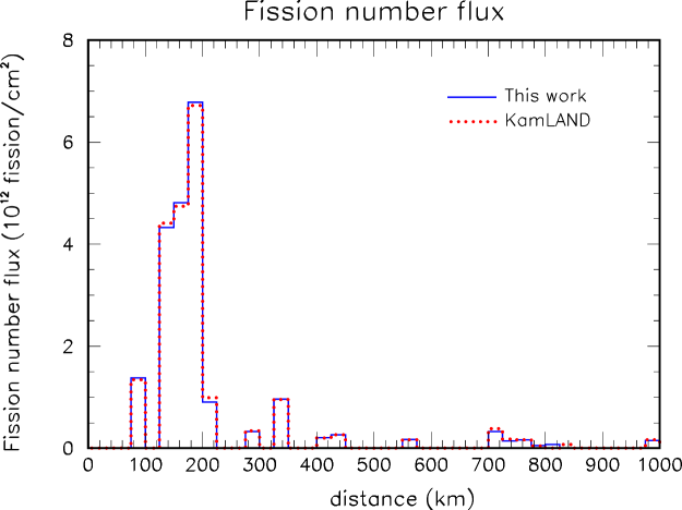
Figure 2: Absolute fission number flux at KamLAND, as a function of the reactor distance. Dotted histogram: KamLAND estimate. Solid histogram: this work.

and its (binned) distribution over the reactor distance $L$. Figure 2 shows that our results are very close to the official KamLAND ones, as taken from Kam3 .

II.2 Detection input

Given the differential neutrino flux in Eq. (5), the time-averaged energy spectrum of reactor events in KamLAND (number of expected events per unit of prompt positron energy $E$) is given by

$$S(E)=\varepsilon\,n\,M\,\Delta t\int dE_{\nu}\,\frac{d\phi}{dE_{\nu}}\int dE^{\prime}\,\frac{d\sigma(E_{\nu},E^{\prime})}{dE^{\prime}}\,r(E,E^{\prime})\ ,$$ (9)

where $\varepsilon=0.898$ is the overall efficiency (after all cuts Kam2 ), $n$ is the target density ($0.848\times 10^{29}$ protons/ton) Kam2 , $r(E,E^{\prime})$ is the energy resolution function (with Gaussian width equal to $7\%(E^{\prime}/\mathrm{MeV})^{1/2}$) Kam3 , and $\sigma$ is the inverse beta decay cross section, estimated as

$$\frac{d\sigma(E_{\nu},E^{\prime})}{dE^{\prime}}\simeq\sigma(E_{\nu})\,\delta(E_{\nu}-E^{\prime}-0.782~{}\mathrm{MeV})\ ,$$ (10)

with $\sigma(E_{\nu})$ taken from Beac . In $r(E,E^{\prime})$, we allow for a systematic offset of the prompt (true) energy scale,

$$E^{\prime}\to E^{\prime}(1+\alpha)\ ,$$ (11)

with standard deviation $\sigma_{\alpha}=2\times 10^{-2}$ Kam2 .

Above the current analysis threshold ($E_{\mathrm{thr}}=2.6$ MeV), we estimate a total of 377.3 reactor events in the absence of oscillations. This value is about $3\%$ higher than the official KamLAND estimate (365.2 events Kam2 ); we obtain a $+3\%$ difference also in comparison with older data Kam1 (89.7 events against the official 86.8 estimate Kam1 ). We have not been able to trace the source of this modest systematic difference, which we choose to compensate “ad hoc” in the following, through a fudge factor $f=0.97$ multiplying the right hand side of Eq. (9).

Finally, one must consider the background energy spectrum $B(E)$ expected over the livetime $\Delta t$. This spectrum has three main components, as described in detail in Kam2 ; Kam3 : the accidental background $B_{1}$, the ⁸He-⁹Li background $B_{2}$, and the ¹³C$(\alpha,n)^{16}$O background $B_{3}$. While $B_{1}$ and $B_{2}$ can be estimated with very small uncertainties Kam2 (that we set to zero), the normalization of the third background is poorly known in both its low-energy ($<5.4$ MeV) and high-energy ($>5.4$ MeV) components Kam3 ($B_{3}^{\prime}$ and $B_{3}^{\prime\prime}$, respectively). We then assume free normalization factors ($\alpha^{\prime}$ and $\alpha^{\prime\prime}$) for such components. In conclusion, we take the absolute background spectrum as

$$B(E)=B_{1}(E)+B_{2}(E)+\alpha^{\prime}B_{3}^{\prime}(E)+\alpha^{\prime\prime}B_{3}^{\prime\prime}(E)\ ,$$ (12)

where the $B_{1}$, $B_{2}$, $B_{3}^{\prime}$ and $B_{3}^{\prime\prime}$ components are taken from Kam3 , while $\alpha^{\prime}$ and $\alpha^{\prime\prime}$ are free (positive) parameters.

II.3 Likelihood function and oscillation parameters

The absolute energy spectrum of events expected above the analysis threshold can always be factorized into the total number of events $N_{\mathrm{theo}}$ times the probability distribution in energy $D(E)$, namely

$$S(E)+B(E)=N_{\mathrm{theo}}\cdot D(E)$$ (13)

with

$$\int_{E_{\mathrm{thr}}}dE\,D(E)=1\ .$$ (14)

We remind that both $N_{\mathrm{theo}}$ and $D(E)$ depend on the systematic energy offset $\alpha$, as well as on the free background parameters $\alpha^{\prime}$ and $\alpha^{\prime\prime}$. In the presence of oscillations, they also depend on the the mass-mixing parameters $(\delta m^{2},\sin^{2}\theta_{12})$.

Given the previous definitions, the first likelihood factor in Eq. (2) can be written as (see also Schw ):

$$\mathcal{L}_{\mathrm{rate}}=\frac{1}{\sqrt{2\pi}\sigma_{\mathrm{rate}}}\exp\left[-\frac{1}{2}\left(\frac{N_{\mathrm{theo}}(\delta m^{2},\,\sin^{2}\theta_{12}\,;\,\alpha,\,\alpha^{\prime},\,\alpha^{\prime\prime})-N_{\mathrm{obs}}}{\sigma_{\mathrm{rate}}}\right)^{2}\right]$$ (15)

where $N_{\mathrm{obs}}=258$ is the total number of observed events Kam2 , and the total error is the sum of the statistical and systematic ($s=6.5\%$ Kam2 ; Kam3 ) uncertainties,

$$\sigma_{\mathrm{rate}}^{2}=N_{\mathrm{theo}}+(s\,N_{\mathrm{theo}})^{2}\ .$$ (16)

The second likelihood factor in Eq. (2) is the product of the probability that the $i$-th event ($i=1,\dots,N_{\mathrm{obs}}$) occurs with the observed energy $E_{i}$,

$$\mathcal{L}_{\mathrm{shape}}=\prod_{i=1}^{\mathrm{258}}D(E_{i}\,|\,\delta m^{2},\,\sin^{2}\theta_{12}\,;\,\alpha,\,\alpha^{\prime},\,\alpha^{\prime\prime})\ ,$$ (17)

where the energy set $\{E_{i}\}$ is given in Kam3 . The third and last likelihood factor in Eq. (2) embeds the penalty for the systematic offset $\alpha$ in Eq. (11),

$$\mathcal{L}_{\mathrm{syst}}=\frac{1}{\sqrt{2\pi}\sigma_{\alpha}}\exp\left[{-\frac{1}{2}\left(\frac{\alpha}{\sigma_{\alpha}}\right)^{2}}\right]\ .$$ (18)

In general, further penalty factors could account for additional KamLAND systematics (not included here for lack of detailed published information).

Finally, the standard $\chi^{2}$ function is obtained as

$$\chi^{2}(\delta m^{2},\sin^{2}\theta_{12})=-2\ln\max_{\{\alpha,\alpha^{\prime},\alpha^{\prime\prime}\}}\mathcal{L}(\delta m^{2},\,\sin^{2}\theta_{12}\,;\,\alpha,\,\alpha^{\prime},\,\alpha^{\prime\prime})\ .$$ (19)

Bounds on the oscillation parameters can be found by plotting isolines of the function

$$\Delta\chi^{2}=\chi^{2}-\min_{\{\delta m^{2},s^{2}_{12}\}}\chi^{2}\ .$$ (20)

The values $\Delta\chi^{2}=4.61$, 5.99, 9.21, and 11.83 correspond to 90, 95, 99, and 99.73% C.L. for two degrees of freedom.

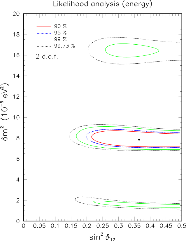
Figure 3: Bounds on the oscillation parameters from a maximum-likelihood analysis of the KamLAND energy spectrum (event-by-event).

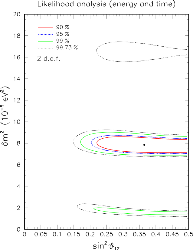
Figure 4: Bounds on the oscillation parameters from a maximum-likelihood analysis of the KamLAND information in energy (event-by-event) and time (monthly binned).

Figure 3 shows the bounds on the oscillation parameters from our likelihood analysis of the KamLAND energy spectrum. The confidence level isolines are in very good agreement with the official ones reported in Fig. 4(a) of Kam2 , modulo the different scales chosen for the axes. These results, together with the previous checks in this Section, demonstrate that we can reproduce, to a good accuracy, both the input and the output of the official KamLAND likelihood analysis of the energy spectrum. This check is also relevant to appreciate, in the next Section, the (small) differences induced by including the time information in the likelihood analysis.

III Likelihood analysis in energy and time

The information reported in File allows to separate the global KamLAND set of 258 event-by-event energies into 23 monthly subsets $I_{m}$,

$$\{E_{i}\}_{i=1,\dots,258}=\bigcup_{m=1,\dots,23}\{E_{i}\}_{i\in I_{m}}\ ,$$ (21)

with corresponding detector livetimes $\Delta t_{m}$. The goal of this section is to include such time information, together with the set of monthly thermal reactor powers $\{P_{jm}^{\mathrm{th}}\}$, into a maximum likelihood analysis. The generalization is straightforward: monthly neutrino fluxes $\phi_{m}$, signal spectra $S_{m}$, background spectra $B_{m}$, and probability distributions $D_{m}$ are defined as

$$\frac{d\phi_{m}}{dE_{\nu}}\simeq\sum_{j=1}^{20}\sum_{f=1}^{4}\frac{P^{\mathrm{th}}_{jm}}{4\pi L_{j}^{2}}\frac{q_{f}}{E_{f}}\frac{dN_{f}}{dE_{\nu}}\ ,$$ (22)

$$S_{m}(E)=\varepsilon\,n\,M\,\Delta t_{m}\int dE_{\nu}\,\frac{d\phi_{m}}{dE_{\nu}}\int dE^{\prime}\,\frac{d\sigma(E_{\nu},E^{\prime})}{dE^{\prime}}\,r(E,E^{\prime})\ ,$$ (23)

$$B_{m}(E)=B(E)\,\frac{\Delta t_{m}}{\Delta t}\ ,$$ (24)

$$S_{m}(E)+B_{m}(E)=N_{\mathrm{theo}}\,D_{m}(E)\ ,$$ (25)

respectively, fulfilling the relations

$$\sum_{m}S_{m}(E) = S(E)\ ,$$ (26)

$$\sum_{m}B_{m}(E) = B(E)\ ,$$ (27)

and the probability normalization condition

$$\sum_{m}\int_{E_{\mathrm{thr}}}dE\,D_{m}(E)=1\ .$$ (28)

The likelihood of the spectral shape information acquires then an explicit (monthly) time dependence,

$$\mathcal{L}_{\mathrm{shape}}=\prod_{m}\,\prod_{i\in I_{m}}D_{m}(E_{i})\ ,$$ (29)

while the functional forms of $\mathcal{L}_{\mathrm{rate}}$ and $\mathcal{L}_{\mathrm{syst}}$ remain the same as in Eqs. (15) and (18), respectively. We have thus all the ingredients to calculate a likelihood function in energy (event-by-event) and time (monthly-binned).

Notice that the likelihood function in energy and time reduces to the energy-only likelihood function in the limit of constant reactor powers $(P_{jm}^{\mathrm{th}}\equiv P_{j}^{\mathrm{th}})$, up to an irrelevant overall factor (the product of $\Delta t_{m}/\Delta t$ ratios); this limit provides a useful cross-check of the numerical results.

III.1 Constraints on the oscillation parameters

We start the discussion of the time-dependent effects in a case where they are (currently) not expected to play a significant role, namely, in the determination of the oscillation parameters $(\delta m^{2},\sin^{2}\theta_{12})$. The KamLAND bounds on these two parameters are basically dominated by two different pieces of information: the energy spectrum shape and its normalization. In particular, the $\delta m^{2}$ parameter governs the oscillation phase, which is strongly constrained by the observation of half-period of oscillations Kam2 ; St05 . This observation is still dominated by statistical errors Berg , which currently hide subleading time-dependent effects, such as a possible shift of the “oscillation dip” for strong reactor power variations (as shown in Fig. 1). On the other hand, the $\sin^{2}\theta_{12}$ parameter governs the oscillation amplitude, whose bounds are dominated by normalization systematics Berg , which are not reduced by adding time information. Therefore, within current uncertainties, we do not expect the mass-mixing bounds from the energy spectrum analysis (Fig. 3) to be significantly changed by adding time information.

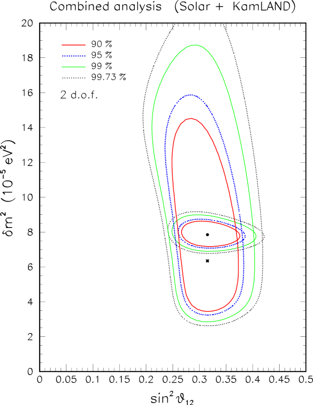
Figure 5: Bounds on the oscillation parameters from all current solar neutrino data Prog , and their combination with the KamLAND bounds in Fig. 4.

Figure 4 shows the results of our likelihood analysis in energy and time, which confirms the above expectations. A comparison with Fig. 3 reveals appreciable changes only in the “high-$\delta m^{2}$” allowed region (so-called LMA-II solution Fo03 ), which appears to be slightly more disfavored by adding time information. This trend allows to exclude with more confidence the LMA-II solution in combination with solar data (which, by themselves, still allow relatively high values of $\delta m^{2}$ SNO2 ). For the sake of completeness, and for later purposes, we show in Fig. 5 the oscillation parameter bounds from our analysis of all current solar neutrino data Prog (including the latest full SNO spectral results SNO2 ) plus the KamLAND likelihood analysis in time and energy. The bounds in Fig. 5 contain, to our knowledge, the largest amount of solar and reactor neutrino information which is publicly available at present.

III.2 Probing time variations of the reactor neutrino flux

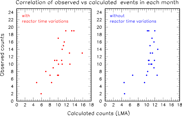
Figure 6: Monthly counts of events observed in KamLAND, plotted against the corresponding theoretical counts (calculated for the global best-fit LMA parameters in Fig. 5). Left panel: time variations of reactor powers included. Right panel: variations excluded (average powers used). The positive correlation between observed and calculated counts appears to be more pronounced in the first case. In both cases, monthly KamLAND livetimes are included.

Variations of the reactor powers and of the livetime efficiency generate time variations of the event rate in KamLAND. Therefore, theoretical event rates including (not including) time information are expected to track more (less) faithfully the observed event rates. In Fig. 6 we plot the observed monthly counts in KamLAND, with respect to our calculated counts, with and without reactor power variations. The comparison of the two panels shows at a glance that the correlation among the 23 points is more evident when monthly reactor powers $(P_{jm}^{\mathrm{theo}})$ are included, with respect to the hypothetical case of constant reactor powers ($P_{jm}^{\mathrm{th}}\equiv P_{j}^{\mathrm{th}})$. Quantitatively, the correlation index decreases from 0.73 (left panel) to 0.58 (right panel). In the right panel, the correlation would be further reduced for hypothetically constant detector livetimes $(\Delta t_{m}=\Delta t/23)$, since all points would then collapse onto a single vertical line (not shown).

The significant covariance between observed and calculated counts—when time information is fully included—suggests that KamLAND is indeed tracking reactor neutrino flux variations. In this sense, Figure 6 qualitatively agrees with the correlation test shown in the first figure of Kam2 . We refrain, however, from fitting a “straight line” through the points in the left panel of Fig. 6, since we know of no clear way to include the point-by-point systematics and the large statistical fluctuations in such a linear fit. A maximum-likelihood test of time variations appears to be more appropriate, both to deal with small monthly counts and to include event-by-event energies and systematics.

In order to test the null hypothesis of no time variations against the hypothesis of actual time variations of the reactor neutrino flux, we introduce an auxiliary variable $\eta$, interpolating between the two cases. In this way, the hypothesis test is transformed into a parameter estimation test Lyon . Formally, we assume that parameter $\eta$ modulates all reactor powers through the equation

$$\tilde{P}_{jm}^{\mathrm{th}}(\eta)=P_{j}^{\mathrm{th}}+\eta\,\Delta P_{jm}^{\mathrm{th}}\ ,$$ (30)

where $\Delta P_{jm}^{\mathrm{th}}=P_{jm}^{\mathrm{th}}-P_{j}^{\mathrm{th}}$ are the actual power variations in each month. Thus $\eta$ continuously “switches on” reactor neutrino flux variations from the null case $\eta=0$ (no time variations) to the real case $\eta=1$ (actual time variations).

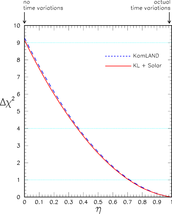
Figure 7: Bounds on the parameter $\eta$, which interpolates between the extreme cases of no time variations of reactor powers ($\eta=0$) and actual time variations of reactor powers ($\eta=1$). The value $\eta=1$ is significantly preferred over $\eta=0$. Bounds at 1, 2, and $3\sigma$ can be obtained at $\Delta\chi^{2}=1$, 4, and 9 (dotted horizontal lines). The results are dominated by the maximum likelihood analysis of KamLAND data in energy and time (dashed line) and are not appreciably affected by including solar neutrino data. The oscillation parameters $(\delta m^{2},\sin^{2}\theta_{12})$ are marginalized in both cases.

By using reactors powers $\tilde{P}_{jm}^{\mathrm{th}}(\eta)$ defined as in the above equation, we build a likelihood function in energy and time $\mathcal{L}(\delta m^{2},\sin^{2}\theta_{12},\eta)$, and marginalize it with respect to the oscillation parameters. The results are shown in Fig. 7, in terms of the function $\Delta\chi^{2}(\eta)$. The hypothetical case of constant averaged reactor powers $(\eta=0)$ is definitely disfavored by KamLAND data, as compared with any case including time variations ($0<\eta<1$). In particular, the difference with respect to the case of actual time variations ($\eta=1$) amounts to about $3\sigma$ ($\Delta\chi^{2}\simeq 9$). We conclude that the results in Fig. 7 (and, to some extent, in Fig. 6) can be taken as a statistically significant indication that reactor neutrino flux variations have been seen in KamLAND.

Finally, it is interesting to note that, in Fig. 7, the addition of solar neutrino information (through an additional $\Delta\chi^{2}$ function which depends on $(\delta m^{2},\sin^{2}\theta_{12})$ but not on $\eta$) does not significantly change the overall bounds on $\eta$. In other words, as also observed in the previous subsection, energy and time information are largely decoupled in KamLAND (at present). The energy information indicates nonzero oscillation parameters, while the time information indicates nonzero variations of the reactor signal rate, with no appreciable cross-talk between these two pieces of information. Only with much smaller errors one might hope to see mixed effects (e.g., time-dependent changes of the energy spectrum dip). However, as we shall see in the next section, such “decoupling” of the oscillation parameters is not necessarily preserved in nonstandard cases, e.g., in a scenario with a hypothetical georeactor.

IV Constraints on the georeactor

It has been proposed Geo1 that there could be enough Uranium in the Earth’s core to naturally start a nuclear fission chain over geological timescales, with a typical power (at the current epoch) of 3–10 TW Geo1 , and possibly up to $\sim 30$ TW Geo2 . The latter value is probably too high to be credible, since the addition of a typical radiogenic contribution of $\sim 20$ TW Fior (not to count other sources Ande ) would exceed the total Earth heat flux (estimated to be $\sim 44$ TW in Poll and recently revised down to $\sim 31$ TW in Hofm ). A georeactor power of $\sim 10$ TW is, however, comparable to the global Earth heat flux uncertainty Ande , and thus cannot be currently excluded by energy-budget arguments. On the other hand, there are independent geochemical and geophysical arguments which seem to disfavor any significant Uranium content in the core McDo . Despite being largely ignored in the Earth science literature, the georeactor hypothesis has attracted some attention in the particle physics literature Geos ; APSR .

In the KamLAND data analysis, a hypothetical georeactor can induce several effects. First, it increases the overall expected event rate. Second, it distorts the spectrum shape, both because its natural fuel composition can be significantly different from that of man-made reactors, and because the oscillation phase for $L=R_{\oplus}$ is different than for $L\sim O(100)$ km. Third, the georeactor signal is constant, while man-made reactors induce, in general, a variable signal in KamLAND. Therefore, we expect that a maximum likelihood analysis of the KamLAND data in energy and time, including the bounds on the oscillation parameters from solar neutrino data, can provide interesting constraints of the georeactor hypothesis. Technically, we implement the georeactor hypothesis by adding (in the KamLAND data analysis) a 21-th reactor at $L=6400$ km, with arbitrary constant power $P_{\mathrm{geo}}$. For definiteness, we assume a current georeactor fuel ratio ${}^{235}\mathrm{U}:{}^{238}\mathrm{U}\simeq 0.75:0.25$, with no significant Pu contribution Geo2 .

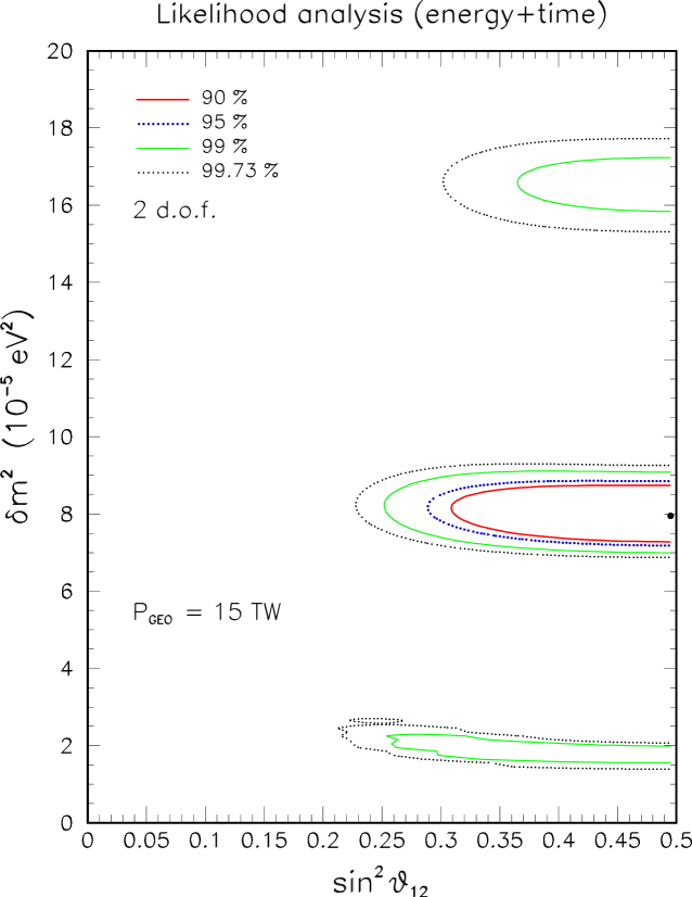
Figure 8: As in Fig. 4, but adding the contribution from a hypothetical georeactor with $P_{\mathrm{geo}}=15$ TW.

Figure 8 shows the bounds on the oscillation parameters from our KamLAND maximum-likelihood analysis in energy and time, for the illustrative case $P_{\mathrm{geo}}=15$ TW. The “wavy” contours of the lowest-$\delta m^{2}$ allowed region in Fig. 8 reflect the “ripples” created by georeactor neutrino oscillations on top the KamLAND energy spectrum (not shown). For the two allowed regions at higher values of $\delta m^{2}$, such (higher-frequency) ripples are smeared away by the finite KamLAND energy resolution, and the contours are smooth. More importantly, all the three allowed regions in Fig. 8 appear to be shifted to larger values of $\sin^{2}\theta_{12}$, as compared with the standard (no georeactor) case in Fig. 4. This behavior is qualitatively expected, since larger mixing is needed to suppress the excess event rate due to the georeactor. For increasing $P_{\mathrm{geo}}$, we should then expect an increasing tension with solar neutrino data, which fix $\sin^{2}\theta_{12}$ around the value $\sim 0.3$ (as shown in Fig. 5) independently of $P_{\mathrm{geo}}$.

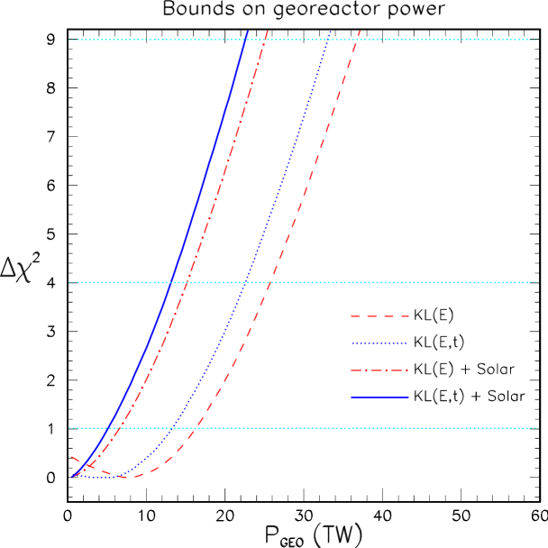
Figure 9: Bounds on the georeactor power from increasingly detailed analyses (with marginalized oscillation parameters). From right to left, the $\Delta\chi^{2}$ curves refer to: KamLAND analysis in energy; KamLAND analysis in energy and time; KamLAND analysis in energy plus solar neutrino data; KamLAND analysis in energy and time, plus solar neutrino data. At 95% C.L. ($2\sigma$), the strongest upper bound (leftmost curve) is $P_{\mathrm{geo}}\lesssim 13$ TW.

Let us now consider the results of a maximum-likelihood analysis where $P_{\mathrm{geo}}$ is free, and the oscillation parameters are marginalized away. The results are shown in Fig. 9, in terms of the function $\Delta\chi^{2}(P_{\mathrm{geo}})$. From right to left, the four curves refer to increasingly informative and powerful analyses: (1) KamLAND likelihood in energy; (2) KamLAND likelihood in energy and time; (3) KamLAND likelihood in energy, plus solar neutrino data; (4) KamLAND likelihood in energy and time, plus solar neutrino data. One can see that solar neutrino data can provide powerful (although indirect) constraints, by forbidding the large values of $\sin^{2}\theta_{12}$ preferred for $P_{\mathrm{geo}}>0$. To a lesser extent, the time information in KamLAND (consistent with known reactor source variations) also disfavor any additional constant georeactor contribution. In all four cases, we find no statistically significant evidence for $P_{\mathrm{geo}}>0$, and can thus place meaningful upper bounds on its value. In particular, the most complete and powerful analysis in Fig. 9 (leftmost curve) provides the bound $P_{\mathrm{geo}}\lesssim 13$ TW at $2\sigma$ (95% C.L.), not too far from the typical expected range of a few TW Geo1 . Basically, such bound tells us that, at $\sim 2\sigma$ level, the georeactor contribution should not exceed twice the KamLAND normalization uncertainty (i.e., $\sim 13\%$).

As a final remark we add that, since known reactor power variations help in constraining a constant (hypothetical) georeactor neutrino flux, they can also be expected to help in constraining the constant (guaranteed Fior ) geoneutrino flux below the current analysis threshold. In other words, as emphasized in Mori , a maximum likelihood analysis in both energy and time should provide a powerful tool for the statistical separation of the expected geoneutrino signal in KamLAND. Similarly, one might try to extend the current bounds on a (hypothetical) constant antineutrino flux from the Sun Anti in the energy region where reactors provide a time-variable signal.

Summarizing, we find that the inclusion of the (monthly-binned) time information in the KamLAND analysis corroborates the usual interpretation of the data, in terms of an oscillation-suppressed neutrino flux generated from known (time-variable) reactor sources. We find no indication for additional constant contribution from a natural georeactor, and place an upper limit $P_{\mathrm{geo}}\lesssim 13$ TW at 95% C.L. In any case, as emphasized in the Introduction, more refined and official KamLAND likelihood analyses (including, e.g., daily data about the detector and the reactors) will be crucial to improve and check such conclusions.

V Conclusions

So far, published KamLAND data analyses have been focussed to the energy spectrum of neutrino events. In this work, after checking that we can reproduce in detail the official KamLAND likelihood analysis in energy, we have tried to add the time information to the analysis. In particular, by including monthly-binned data on Japanese reactor powers, KamLAND event-by-event energies, and detector livetimes, we find that the case of actual time variations of reactor powers is significantly preferred ($\sim 3\sigma$) over the hypothetical case of no time variations. This interesting indication is basically unaltered by adding solar neutrino constraints on the oscillation parameters. We have also considered the effect of a hypothetical georeactor with power $P_{\mathrm{geo}}$ in the analysis. We find increasingly tighter upper bounds as more data (from time variations and from solar neutrinos) are included, down to $P_{\mathrm{geo}}\lesssim 13$ TW at 95% C.L.

Our analysis supports the standard interpretation of the observed KamLAND neutrino events as generated by known reactors sources and affected by flavor oscillations with mass-mixing parameters consistent with solar neutrino data. Implications for a hypothetical constant neutrino source in the Earth interior (the georeactor) start to emerge. Other constant-flux sources (e.g., geoneutrinos or solar antineutrinos) might be usefully constrained in a similar way. We hope that these encouraging results may motivate other independent analyses of the reactor information in the time domain, especially by the KamLAND collaboration that, by using the complete and fully controlled data set, can certainly provide more reliable results and explore interesting new facets of the topics touched in this work.

- (1) A. Suzuki, in the Proceedings of the Nobel Symposium on Neutrino Physics (Haga Slott, Enköping, Sweden, 2004) ed. by L. Bergström, O. Botner, P. Carlson, P.O. Hulth, and T. Ohlsson, to appear in Physica Scripta (2005). Slides available at: www.physics.kth.se/nobel2004 .
- (2) G. Gratta, talk at Neutrino 2004, 21st International Conference on neutrino Physics and Astrophysics (Paris, France, 2004). Slides available at: neutrino2004.in2p3.fr .
- (3) B. Pontecorvo, Zh. Eksp. Teor. Fiz. 53, 1717 (1968) [Sov. Phys. JETP 26, 984 (1968)].
- (4) Z. Maki, M. Nakagawa, and S. Sakata, Prog. Theor. Phys. 28, 870 (1962).
- (5) C. Bemporad, G. Gratta, and P. Vogel, Rev. Mod. Phys. 74, 297 (2002).
- (6) KamLAND Collaboration, K. Eguchi et al., Phys. Rev. Lett. 90, 021802 (2003).
- (7) KamLAND Collaboration, K. Eguchi et al., Phys. Rev. Lett. 94, 081801 (2005).
- (8) KamLAND 2nd data release, www.awa.tohoku.ac.jp/KamLAND/datarelease/2ndresult.html .
- (9) L. Wolfenstein, in Neutrino ’78, 8th International Conference on Neutrino Physics and Astrophysics (Purdue U., West Lafayette, Indiana, 1978), ed. by E.C. Fowler (Purdue U. Press, 1978), p. C3.
- (10) L. Wolfenstein, Phys. Rev. D 17, 2369 (1978); S.P. Mikheev and A.Yu. Smirnov, Yad. Fiz. 42, 1441 (1985) [Sov. J. Nucl. Phys. 42, 913 (1985)].
- (11) J.N. Bahcall, Neutrino Astrophysics (Cambridge University Press, Cambridge, UK, 1989).
- (12) Homestake Collaboration, B.T. Cleveland, T. Daily, R. Davis Jr., J.R. Distel, K. Lande, C.K. Lee, P.S. Wildenhain, and J. Ullman, Astrophys. J. 496, 505 (1998).
- (13) SAGE Collaboration, J.N. Abdurashitov et al., J. Exp. Theor. Phys. 95, 181 (2002) [Zh. Eksp. Teor. Fiz. 95, 211 (2002)].
- (14) T. Kirsten for the GALLEX/GNO Collaboration, in the Proceedings of Neutrino 2002, 20th International Conference on Neutrino Physics and Astrophysics (Munich, Germany, 2002), edited by F. von Feilitzsch and N. Schmitz, Nucl. Phys. B Proc. Suppl. 118, 33 (2003).
- (15) GNO Collaboration, M. Altmann et al., hep-ex/0504037.
- (16) SK Collaboration, M.B. Smy et al., Phys. Rev. D 69, 011104 (2004).
- (17) SNO Collaboration, S.N. Ahmed et al., Phys. Rev. Lett. 92, 181301 (2004).
- (18) SNO Collaboration, B. Aharmim et al., nucl-ex/0502021.
- (19) Review of Particle Physics, S. Eidelman et al., Phys. Lett. B 592, 1 (2004).
- (20) E. Lisi, A. Palazzo, and A.M. Rotunno, Astropart. Phys. 21, 511 (2004).
- (21) J.M. Herndon, Proc. Natl. Acad. Sci. U.S.A. 93(2), 646 (1996); ibidem 100(6), 3047 (2003); see also the website www.nuclearplanet.com .
- (22) K. Inoue, private communication (2003).
- (23) G.L. Fogli, E. Lisi, A. Marrone, D. Montanino, A. Palazzo, and A.M. Rotunno, Phys. Rev. D 67, 073002 (2003).
- (24) A. Ianni, J. Phys. G 29, 2107 (2003).
- (25) T. Schwetz, Phys. Lett. B 577, 120 (2003).
- (26) G. Fiorentini, T. Lasserre, M. Lissia, B. Ricci and S. Schönert, Phys. Lett. B 558, 15 (2003).
- (27) P.C. de Holanda and A.Yu. Smirnov, JCAP 0302, 001 (2003).
- (28) J.N. Bahcall, M.C. Gonzalez-Garcia, and C. Peña-Garay, JHEP 0408, 016 (2004).
- (29) M. Maltoni, T. Schwetz, M.A. Tortola, and J.W.F. Valle, New J. Physics 6, 122 (2004).
- (30) P. Aliani, V. Antonelli, M. Picariello, and E. Torrente-Lujan, Phys. Rev. D 013005 (2004).
- (31) A.B. Balantekin, V. Barger, D. Marfatia, S. Pakvasa, and H. Yuksel, Phys. Lett. B 608, 115 (2005).
- (32) A. Bandyopadhyay, S. Choubey, S. Goswami, S.T. Petcov, and D.P. Roy, Phys. Lett. B 608, 115 (2005).
- (33) A. Strumia and F. Vissani, hep-ph/0503246.
- (34) Japan Atomic Industrial Forum, www.jaif.or.jp/english/aij/index2.html (Operating Records of Nuclear Power Plants in Japan). The information on this web page was free until March 2005; currently it requires subscription.
- (35) Monthly-binned KamLAND data on the detector livetime and on event-by-event energies are summarized in the file monthly_sort_energy.dat, currently available at Kam3 .
- (36) Proposal for U.S. participation in KamLAND, available at: kamland.lbl.gov/TalksPaper .
- (37) F. Bohem and P. Vogel, Physics of Massive Neutrinos (Cambridge University Press, New York, 1992).
- (38) H. Murayama and A. Pierce, Phys. Rev. D 65, 013012 (2002).
- (39) P. Vogel and J. Engel, Phys. Rev. D 39, 3378 (1989).
- (40) P. Vogel and J. Beacom, Phys. Rev. D 60, 053003 (1999).
- (41) G.L. Fogli, E. Lisi and D. Montanino, Phys. Rev. D 54, 2048 (1996).
- (42) B. Berger, in the 40th Rencontres de Moriond, Electroweak Interactions and Unified Theories (La Thuile, Italy, 2005). Slides available at: moriond.in2p3.fr/EW/2005 .
- (43) G.L. Fogli, E. Lisi, A. Marrone, and A. Palazzo, work in progress.
- (44) L. Lyons, “Selecting between two hypotheses,” Oxford University Report No. OUNP-99-12.
- (45) J.M. Herndon and D. A. Edgerley, hep-ph/0501216.
- (46) See G. Fiorentini, M. Lissia, F. Mantovani and R. Vannucci, hep-ph/0501111, and references therein.
- (47) D. Anderson, “Energetics of the Earth and the missing heat source mistery,” available at www.mantleplumes.org/Energetics.html .
- (48) H.N. Pollack, S.J. Hurter, and J.R. Johnson, Rev. Geophys. 31, 267 (1993).
- (49) A.M. Hofmeister and R.E. Criss, Tectonophysics 395, 159 (2005).
- (50) W.F. McDonough, Compositional Models for the Earth’s Core, in “Treatise on Geochemistry,” Vol. II, edited by R.W. Carlson (Elsevier-Pergamon, Oxford, 2003); website: www.treatiseongeochemistry.com .
- (51) See, e.g., R.S. Raghavan, hep-ex/0208038; R.J. de Meijer, E.R. van der Graaf, and K.P. Jungmann, physics/0404046; G. Domogatski, V. Kopeikin, L. Mikaelian, and V. Sinev, hep-ph/0407148.
- (52) American Physical Society, Multidivisional Neutrino Study: Report of the Reactor Working Group (2004), available at www.aps.org/neutrino .
- (53) G.L. Fogli, E. Lisi, A. Palazzo and A. M. Rotunno, hep-ph/0405139.
- (54) KamLAND Collaboration, K. Eguchi et al., Phys. Rev. Lett. 92, 071301 (2004).