Cosmological Family Asymmetry and CP violation

Abstract

We discuss how the cosmological baryon asymmetry can be achieved by the lepton family asymmetries of heavy Majorana neutrino decays and they are related to CP violation in neutrino oscillation, in the minimal seesaw model with two heavy Majorana neutrinos. We derive the most general formula for CP violation in neutrino oscillation in terms of the heavy Majorana masses and Yukawa mass term. It is shown that the formula is very useful to classify several models in which $e-$, $\mu-$ and $\tau-$leptogenesis can be separately realized and to see how they are connected with low energy CP violaton. To make the models predictive, we take texture with two zeros in the Dirac neutrino Yukawa matrix. In particular, we find some interesting cases in which CP violation in neutrino oscillation can happen while lepton family asymmetries do not exist at all. On the contrary, we can find $e-$, $\mu-$ and $\tau-$leptogenesis scenarios in which the cosmological CP violation and low energy CP violation measurable via neutrino oscillations are very closely related to each other. By determining the allowed ranges of the parameters in the models, we predict the sizes of CP violation in neutrino oscillation and $|V_{e3}^{MNS}|$. Finally, the leptonic unitarity triangles are reconstructed.

I Introduction

CP violations in the neutrino seesaw models have recently attracted much attention because the measurements of CP violation via neutrino oscillation are being planned in future experiments and there may exist a connection between the low energy neutrino CP violation and the matter and anti-matter asymmetry of the universe through the leptogenesis scenario in the seesaw models [1]. In contrast to the quark sector, since the number of independent CP violating phases in the neutrino seesaw models is more than one[2], it is not straightforward to discriminate the CP violating phases contributing to the leptogenesis from the low energy experiments [3]. One can show that the CP violation phases at high energy can contribute to the low energy effective Majorana mass matrix and thus they may be concerned with a CP violating phase called $\delta$ in the standard parametrization of MNS matrix, which is measurable from CP violation in neutrino oscillation. One might think that non-zero $\delta$ may play a role in CP violation for leptogenesis in the neutrino seesaw models. However, this is not always the case, because several independent CP phases contribute to both the leptogenesis CP violation at high energy and CP violation of neutrino oscillation at low energy. There is the case in which while at low energy the total effect of many CP phases are cancelled but at high energy cosmological CP violation remains. There is the opposite case in which the cosmological CP violation vanishes while CP violation at low energy is non-zero. Considering the situation, it is important to study CP violation phenomena as much as possible both at high energy and low energy. In the previous work [4], it was shown that the lepton family asymmetries $Y_{e}$,$Y_{\mu}$ and $Y_{\tau}$ which are generated by heavy Majorana neutrinos decays are sensitive to one of the many CP violating phases. Though the total lepton asymmetry $Y=Y_{e}+Y_{\mu}+Y_{\tau}$ remains as a constant, flavor composition of the asymmetries $Y_{e}:Y_{\mu}:Y_{\tau}$ can vary by changing the phase. As a particulary interesting case, the amount and the sign of each lepton family asymmetry $Y_{i}$ can be very different from the total lepton asymmetry as $|Y|\ll|Y_{\mu}|,|Y_{\tau}|$. One can also find the case [4], the lepton asymmetry $Y$ could be dominated by a particular lepton family asymmetry as $Y\sim Y_{\mu}$ or $Y\sim Y_{\tau}$. If this is the case, it indicates the interesting scenario of baryogenesis that the matter in the present universe was originated by the second or the third family of leptons. Interestingly, the models proposed in [5] correspond to the $\mu$ or $\tau$ family number dominant leptogenesis scenarios. In this work, we study how such scenario can be probed by low energy flavor violating processes such as neutrino oscillations. The paper is organized as follows. In section II, we study how CP violating phases are related to lepton family asymmetries. The reason why, in general, the family asymmetries can be different from the total lepton number asymmetry is shown in a comprehensive way. Then we show how they have some impact on the CP violation in the neutrino mixings by deriving the formula for low energy CP violation neutrino mixings in terms of the fundamental parameters for the minimal seesaw model. The analytical formulae for MNS matrix are given both for normal and inverted cases. In section III, we focus on the textures with two zeros in Yukawa mass terms. By using the mixing angles and mass squared diffrences determined by neutrino oscillation experiments, we determine the parameters of the models and make prediction on $|V_{e3}^{MNS}|$ and CP violation in neutrino oscillation. Based on this numerical fit, we reconstruct the leptonic unitarity triangles. Section IV is devoted to summary and discussion.

II CP violation related to the lepton family asymmetry

We start with the lepton family asymmetries generated from heavy Majorana neutrino decays, which are defined by [4],

$$\epsilon_{i}^{k}=\frac{\Gamma[N^{k}\rightarrow l_{i}^{-}\phi^{+}]-\Gamma[N^{k}\rightarrow l_{i}^{+}\phi^{-}]}{\Gamma[N^{k}\rightarrow l_{i}^{-}\phi^{+}]+\Gamma[N^{k}\rightarrow l_{i}^{+}\phi^{-}]},$$ (1)

where $i=(e,\mu,\tau)$ and $N^{k}$ denotes $k-$ th heavy Majorana neutrino. The total lepton number asymmetry from $N^{k}$ is [1],

$$\epsilon^{k}=\sum_{i=e,\mu,\tau}\epsilon_{i}^{k}{\rm Br}(N^{k}\rightarrow{l_{i}}^{\pm}\phi^{\mp}),$$ (2)

where ${\rm Br}$ denotes the tree level branching fraction. For our purpose, let us focus on the seesaw model with two heavy Majorana neutrinos [5][6][7][8],

$${\cal L}_{m}=-y_{\nu}^{ik}\overline{L_{i}}N_{k}\tilde{\phi}-y_{l}^{i}\overline{L_{i}}l_{R_{i}}{\phi}-\frac{1}{2}\overline{N_{k}}^{c}M_{k}N_{k}+h.c.,$$ (3)

where $i=e,\mu,\tau$ and $k=1,2$. $L_{i},l_{R},\phi$ are $SU(2)$ lepton doublet fields, charged lepton singlet fields and Higgs scalar, respectively. Here we take a basis in which both charged lepton and singlet Majorana neutrino mass matrices are real and diagonal. In this basis, the lepton family asymmetries given in Eq.(1) can be written as [4],

$$\epsilon_{i}^{k} = \frac{1}{8\pi}\sum\limits_{k^{\prime}\neq k}\left[I(x_{k^{\prime}k})\frac{{\rm Im}[(y_{\nu}^{\dagger}y_{\nu})_{kk^{\prime}}(y_{\nu})^{*}_{ik}(y_{\nu})_{ik^{\prime}}]}{|(y_{\nu})_{ik}|^{2}}\right.$$ (4)

$$\left.+\frac{1}{1-x_{k^{\prime}k}}\frac{{\rm Im}[(y_{\nu}^{\dagger}y_{\nu})_{k^{\prime}k}(y_{\nu})^{*}_{ik}(y_{\nu})_{ik^{\prime}}]}{|(y_{\nu})_{ik}|^{2}}\right],$$

where $x_{k^{\prime}k}=\frac{M_{k^{\prime}}^{2}}{M^{2}_{k}}$ and $I(x)$ is given as [1][9],

$$I(x) = \sqrt{x}\left[1+\frac{1}{1-x}+(1+x)\ln\frac{x}{1+x}\right]$$ (7)

$$= \left\{\begin{array}[]{ll}-\frac{3}{2}x^{-1/2}&\ \ \ {\rm for}\ \ x\gg 1,\\ -2x^{3/2}&\ \ \ {\rm for}\ \ x\ll 1.\end{array}\right.$$

It is convenient to write $3\times 2$ matrix Dirac mass $m_{D}=y_{\nu}\frac{v}{\sqrt{2}}$ as,

$$m_{D}=\left(\begin{array}[]{cc}{\bf m_{D1}},&{\bf m_{D2}}\end{array}\right)=\left(\begin{array}[]{cc}m_{De1}&m_{De2}\\ m_{D\mu 1}&m_{D\mu 2}\\ m_{D\tau 1}&m_{D\tau 2}\end{array}\right)=\left(\begin{array}[]{cc}{\bf u_{1}},{\bf u_{2}}\end{array}\right)\left(\begin{array}[]{cc}m_{D1}&0\\ 0&m_{D2}\end{array}\right),$$ (15)

where two unit vectors are introduced,

$${\bf u_{i}}=\frac{\bf m_{Di}}{m_{Di}},$$ (16)

with $m_{Di}=|{\bf m_{Di}}|$. Without loss of generality, we can take ${\bf u_{1}}$ and ${\bf u_{2}}$ to be real and complex, respectively. Then, three CP violating phases correspond to arg($u_{2i}$) ($i=e$, $\mu$, and $\tau$). With the definitions, one can write,

$${\rm Br}(N^{k}\rightarrow{l_{i}}^{\mp}\phi^{\pm})=|u_{ik}|^{2},$$

$$\epsilon_{i}^{1}{\rm Br}(N^{1}\rightarrow{l_{i}}^{\mp}\phi^{\pm})=$$

$$\frac{(m_{D2})^{2}}{4\pi v^{2}}\left(I\left(\frac{M_{2}^{2}}{M_{1}^{2}}\right){\rm Im}[({\bf u_{1}^{\dagger}\cdot u_{2}})u_{i1}^{\ast}u_{i2}]+\frac{M_{1}^{2}}{M_{1}^{2}-M_{2}^{2}}{\rm Im}[({\bf u_{1}^{\dagger}\cdot u_{2}})^{\ast}u_{i1}^{\ast}u_{i2}]\right),$$

$$\epsilon_{i}^{2}{\rm Br}(N^{2}\rightarrow{l_{i}}^{\mp}\phi^{\pm})=$$

$$-\frac{(m_{D1})^{2}}{4\pi v^{2}}\left(I\left(\frac{M_{1}^{2}}{M_{2}^{2}}\right){\rm Im}[({\bf u_{1}^{\dagger}\cdot u_{2}})u_{i1}^{\ast}u_{i2}]+\frac{M_{2}^{2}}{M_{2}^{2}-M_{1}^{2}}{\rm Im}[({\bf u_{1}^{\dagger}\cdot u_{2}})^{\ast}u_{i1}^{\ast}u_{i2}]\right).$$

(17)

It is interesting to note that the lepton family asymmetries are related to the following combinations of Yukawa terms,

$$A_{12}^{e}=({\bf u_{1}^{\dagger}\cdot u_{2}}){u}_{e1}^{\ast}{u}_{e2},$$

$$A_{12}^{\mu}=({\bf u_{1}^{\dagger}\cdot u_{2}}){u}_{\mu 1}^{\ast}{u}_{\mu 2},$$

$$A_{12}^{\tau}=({\bf u_{1}^{\dagger}\cdot u_{2}}){u}_{\tau 1}^{\ast}{u}_{\tau 2},$$ (18)

$$B_{12}^{e}=({\bf u_{1}^{\dagger}\cdot u_{2}})^{\ast}{u}_{e1}^{\ast}{u}_{e2},$$

$$B_{12}^{\mu}=({\bf u_{1}^{\dagger}\cdot u_{2}})^{\ast}{u}_{\mu 1}^{\ast}{u}_{\mu 2},$$

$$B_{12}^{\tau}=({\bf u_{1}^{\dagger}\cdot u_{2}})^{\ast}{u}_{\tau 1}^{\ast}{u}_{\tau 2},$$ (19)

where $A_{12}^{i}=B_{12}^{i}\exp(2i\gamma)$ with $\gamma={\rm arg}({\bf u_{1}^{\dagger}\cdot u_{2}})$. In addition, $A_{12}$ and $B_{12}$ satisfy the following sum rules,

$$A_{12}^{e}+A_{12}^{\mu}+A_{12}^{\tau}=({\bf u_{1}^{\dagger}\cdot u_{2}})^{2},$$

$$B_{12}^{e}+B_{12}^{\mu}+B_{12}^{\tau}=|({\bf u_{1}^{\dagger}\cdot u_{2}})|^{2}.$$ (20)

The relations are shown in Fig.1, where $\gamma=\frac{\pi}{4}$ is taken. They are quadrangles in complex plane. The imaginary part of $A$ is related to CP asymmetry of leptogenesis.

Figure 1: Schematic view of quadrangles.

The ratios of lepton family asymmetry to the total lepton asymmetry are written as;

$$\frac{\epsilon^{1}_{i}}{\epsilon^{1}} = \frac{I(\frac{M_{2}^{2}}{M_{1}^{2}}){\rm Im}A_{12}^{i}+\frac{M_{1}^{2}}{M_{1}^{2}-M_{2}^{2}}{\rm Im}B_{12}^{i}}{I(\frac{M_{2}^{2}}{M_{1}^{2}})({\rm Im}A_{12}^{e}+{\rm Im}A_{12}^{\mu}+{\rm Im}A_{12}^{\tau})},$$

$$\frac{\epsilon^{2}_{i}}{\epsilon^{2}} = \frac{I(\frac{M_{1}^{2}}{M_{2}^{2}}){\rm Im}A_{21}^{i}+\frac{M_{2}^{2}}{M_{2}^{2}-M_{1}^{2}}{\rm Im}B_{21}^{i}}{I(\frac{M_{1}^{2}}{M_{2}^{2}})({\rm Im}A_{21}^{e}+{\rm Im}A_{21}^{\mu}+{\rm Im}A_{21}^{\tau})}.$$ (21)

In the model with two heavy Majorana neutrinos $N_{1}$ and $N_{2}$ with large hierarchical mass, e.g., $M_{1}\ll M_{2}$, the family asymmetries from the lightest heavy Majorana neutrinos decay are approximately given as,

$$\frac{\epsilon^{1}_{e}}{\epsilon^{1}}\approx \frac{{\rm Im}A_{12}^{e}}{{\rm Im}(A_{12}^{e}+A_{12}^{\mu}+A_{12}^{\tau})},$$

$$\frac{\epsilon^{1}_{\mu}}{\epsilon^{1}}\approx \frac{{\rm Im}A_{12}^{\mu}}{{\rm Im}(A_{12}^{e}+A_{12}^{\mu}+A_{12}^{\tau})},$$

$$\frac{\epsilon^{1}_{\tau}}{\epsilon^{1}}\approx \frac{{\rm Im}A_{12}^{\tau}}{{\rm Im}(A_{12}^{e}+A_{12}^{\mu}+A_{12}^{\tau})}.$$

Therefore one-family dominant leptogenesis can be realized when the quadrangle is replaced by a line which is determined by one of $A^{e}_{12},A^{\mu}_{12}$ and $A^{\tau}_{12}$ with a non-trivial CP violating phase. If this is the case, the imaginary parts of $A^{e}_{12}$, $A^{\mu}_{12}$ and $A^{\tau}_{12}$ are related to e-leptogenesis, $\mu$-leptogenesis and $\tau$-leptogenesis, respectively. We also note that the imaginary part of $\sum_{a}A^{a}$ can be smaller than the imaginary part of $A^{a}$. If this is the case, each family asymmetry is much larger than the total lepton asymmetry. Now let us discuss how the family asymmetry is related to the CP violation in neutrino oscillations,

$$P(\nu_{\mu}\to\nu_{e})-P(\bar{\nu_{\mu}}\to\bar{\nu_{e}})=4J\left(\sin\frac{\Delta m_{12}^{2}L}{2E}+\sin\frac{\Delta m_{23}^{2}L}{2E}+\sin\frac{\Delta m_{31}^{2}L}{2E}\right),$$ (23)

where $J$ is Jarlskog invariant [10] defined as,

$$J={\rm Im}\left(V^{MNS}_{e1}V^{MNS\ast}_{\mu 1}V^{MNS\ast}_{e2}V^{MNS}_{\mu 2}\right).$$ (24)

In the basis where the charged lepton mass matrix is diagonal, $J$ is related to the following quantity [3],

$$\Delta={\rm Im}\left((m_{eff}m_{eff}^{\dagger})_{e\mu}(m_{eff}m_{eff}^{\dagger})_{\mu\tau}(m_{eff}m_{eff}^{\dagger})_{\tau e}\right),$$ (25)

where $m_{eff}=-m_{D}\frac{1}{M}m_{D}^{T}$, and the relation between $J$ and $\Delta$ is given as,

$$J=\frac{\Delta}{(n_{1}^{2}-n_{2}^{2})(n_{2}^{2}-n_{3}^{2})(n_{3}^{2}-n_{1}^{2})},$$ (26)

where $n_{i}^{2}$ are three mass eigenvalues of $m_{eff}m_{eff}^{\dagger}$. To facilitate the calculation of $\Delta$, we introduce three $2\times 2$ hermitian matrices $H_{e}$,$H_{\mu}$ and $H_{\tau}$,

$$H_{i}=\left(\begin{array}[]{cc}\frac{|m_{Di1}|^{2}}{M_{1}}&\frac{m_{Di1}m_{Di2}^{\ast}}{\sqrt{M_{1}M_{2}}}\\ \frac{m_{Di1}^{\ast}m_{Di2}}{\sqrt{M_{1}M_{2}}}&\frac{|m_{Di2}|^{2}}{M_{2}}\end{array}\right),\quad(i=e,\mu,\tau),$$ (29)

and $\Delta$ is obtained by simply taking trace of the product of $H$s,

$$\Delta={\rm ImTr}\left({H^{\ast}H_{e}H^{\ast}H_{\mu}H^{\ast}H_{\tau}}\right),$$ (30)

with $H=H_{e}+H_{\mu}+H_{\tau}$. The formula given in terms of $2\times 2$ matrices $H$ is useful and can be generalized to the seesaw model including any number ($n_{M}$) of heavy Majorana neutrinos by replacing $2\times 2$ matrices $H$ in Eq.(29) by $n_{M}\times n_{M}$ matrices. Eq.(30) shows that CP violations in neutrino oscillation is related to the imaginary part of $H_{e12}$, $H_{\mu 12}$ and $H_{\tau 12}$. We introduce the following parameters with mass dimension,

$$X_{i}=\frac{m_{Di}^{2}}{M_{i}},\quad(i=1,2).$$ (31)

By substituting Eq.(29) into Eq.(30), we obtain,

$$\Delta= \left(1-{\bf|u_{1}^{\dagger}\cdot u_{2}|^{2}}\right)\times$$

$$\Biggl{(}X_{1}^{4}X_{2}^{2}\left({\rm Im}[\left(u_{e1}^{\ast}u_{e2}u_{\mu 1}u_{\mu 2}^{\ast}\right)|u_{\tau 1}|^{2}+\left(u_{\mu 1}^{\ast}u_{\mu 2}u_{\tau 1}u_{\tau 2}^{\ast}\right)|u_{e1}|^{2}+\left(u_{\tau 1}^{\ast}u_{\tau 2}u_{e1}u_{e2}^{\ast}\right)|u_{\mu 1}|^{2}]\right)$$

$$+X_{1}^{3}X_{2}^{3}\left({\rm Im}[(u_{e1}^{\ast}u_{e2})({\bf u_{1}^{\dagger}\cdot u_{2}})(|u_{\tau 1}u_{\mu 2}|^{2}-|u_{\mu 1}u_{\tau 2}|^{2})\right.$$

$$\left.\qquad\qquad\qquad\qquad+(u_{\mu 1}^{\ast}u_{\mu 2})({\bf u_{1}^{\dagger}\cdot u_{2}})(|u_{e1}u_{\tau 2}|^{2}-|u_{\tau 1}u_{e2}|^{2})\right.$$

$$\left.\qquad\qquad\qquad\qquad+(u_{\tau 1}^{\ast}u_{\tau 2})({\bf u_{1}^{\dagger}\cdot u_{2}})(|u_{\mu 1}u_{e2}|^{2}-|u_{e1}u_{\mu 2}|^{2})]\right)$$

$$-X_{1}^{2}X_{2}^{4}\left({\rm Im}[\left(u_{e1}^{\ast}u_{e2}u_{\mu 1}u_{\mu 2}^{\ast}\right)|u_{\tau 2}|^{2}+\left(u_{\mu 1}^{\ast}u_{\mu 2}u_{\tau 1}u_{\tau 2}^{\ast}\right)|u_{e2}|^{2}+\left(u_{\tau 1}^{\ast}u_{\tau 2}u_{e1}u_{e2}^{\ast}\right)|u_{\mu 2}|^{2}]\right)\Biggr{)}.$$

This is the most general formula to express the low energy CP violation measurable via neutrino oscillation in terms of the Majorana masses and the Yukawa terms in the seesaw model and a main result of the paper. In the model with two heavy Majorana neutrinos, the same quantity is computed by within two zeros texture models in [5]. For the most general case, $J$ is obtained by using bi-unitary parametrization of $m_{D}$ [6]. It is worthwhile to note that the terms proportional to $X_{1}^{3}X_{2}^{3}$ are related to the family asymmetries because they are proportional to ${\rm Im}A_{12}^{e},{\rm Im}A_{12}^{\mu}$ and ${\rm Im}A_{12}^{\tau}$. However, the terms proportional to $X_{1}^{4}X_{2}^{2}$ and $X_{1}^{2}X_{2}^{4}$ are not directly related to ${\rm Im}A^{a}$. Now, let us study the following two interesting cases.
(1) ${\bf u_{1}^{\dagger}\cdot u_{2}}=0$.
This corresponds to the case that there is no leptogenesis and any family asymmetries are vanishing. However, CP violation in neutrino oscillation can occur in this case because $\Delta$ is not vanishing,

$$\Delta=X_{1}^{2}X_{2}^{2}(X_{1}^{2}-X_{2}^{2}){\rm Im}\left(u_{\tau 1}^{\ast}u_{\tau 2}u_{e1}u_{e2}^{\ast}\right).$$ (33)

(2) ${\bf u_{1}^{\dagger}\cdot u_{2}}=u_{1a}^{\ast}u_{2a}\quad(a=e,\mu,\tau)$.
Each case for $a$ corresponds to one family dominant leptogenesis, such as e-leptogenesis, $\mu$-letogenesis or $\tau$-leptogenesis. This implies that the lepton asymmetry is dominated by one particular family asymmetry. In order to see how the scenarios of leptogenesis are connected with the low energy CP violation parametrized by $\Delta$, we consider the Dirac neutrino Yukawa matrix containing two zeros which makes the scenarios more predictable. In this class of the models, the light neutrino mass matrix given by $m_{eff}$ can be parametrized by five independent parameters. From the experimental results on three mixing angles and two mass squared differences, the five parameters including a CP phase are strongly constrained. In table 1 and table 2, we classify the models with two zeros texture into type I and II depending on the positions of the two zeros in the neutrino Dirac Yukawa matrix. As one can see from table 1, for type I models, $\Delta$ is generally non-vanishing and proportional to ${{\rm Im}}(u_{a1}^{\ast}u_{a2})^{2}$, which implies that there exists a strong correlation between low energy CP violation and leptogenesis. In contrast to the type I models, for the type II models, the low energy CP violating parameter $\Delta$ is vanishing and thus it is difficult to trace the origin of cosmological family asymmetries from the measurement of the CP violation in neutrino oscillation.

Table 1: Type I texture models and low energy CP violation

Type		$\Delta$
Type I (a) e-leptogenesis	$\left(\begin{array}[]{cc}u_{e1}&u_{e2}\\ u_{\mu 1}&0\\ 0&u_{\tau 2}\\ \end{array}\right)$	$(1-|u_{e1}u_{e2}|^{2})X_{1}^{3}X_{2}^{3}{\rm Im}(u_{e1}^{\ast}u_{e2})^{2}(-|u_{\tau 2}|^{2}|u_{\mu 1}|^{2})$
Type I(b) e-leptogenesis	$\left(\begin{array}[]{cc}u_{e1}&u_{e2}\\ 0&u_{\mu 2}\\ u_{\tau 1}&0\end{array}\right)$	$(1-|u_{e1}u_{e2}|^{2})X_{1}^{3}X_{2}^{3}{\rm Im}(u_{e1}^{\ast}u_{e2})^{2}|u_{\tau 1}|^{2}|u_{\mu 2}|^{2}.$
Type I (a) $\mu$ leptogenesis	$\left(\begin{array}[]{cc}u_{e1}&0\\ u_{\mu 1}&u_{\mu 2}\\ 0&u_{\tau 2}\\ \end{array}\right)$	$(1-|u_{\mu 1}u_{\mu 2}|^{2})X_{1}^{3}X_{2}^{3}{\rm Im}(u_{\mu 1}^{\ast}u_{\mu 2})^{2}(|u_{\tau 2}|^{2}|u_{e1}|^{2})$
Type I (b) $\mu$ leptogenesis	$\left(\begin{array}[]{cc}0&u_{e2}\\ u_{\mu 1}&u_{\mu 2}\\ u_{\tau 1}&0\\ \end{array}\right)$	$(1-|u_{\mu 1}u_{\mu 2}|^{2})X_{1}^{3}X_{2}^{3}{\rm Im}(u_{\mu 1}^{\ast}u_{\mu 2})^{2}(-|u_{e2}|^{2}|u_{\tau 1}|^{2})$
Type I (a) $\tau$ leptogenesis	$\left(\begin{array}[]{cc}u_{e1}&0\\ 0&u_{\mu 2}\\ u_{\tau 1}&u_{\tau 2}\\ \end{array}\right)$	$(1-|u_{\tau 1}u_{\tau 2}|^{2})X_{1}^{3}X_{2}^{3}{\rm Im}(u_{\tau 1}^{\ast}u_{\tau 2})^{2}(-|u_{e1}|^{2}|u_{\mu 2}|^{2})$
Type I (b) $\tau$ leptogenesis	$\left(\begin{array}[]{cc}0&u_{e2}\\ u_{\mu 1}&0\\ u_{\tau 1}&u_{\tau 2}\end{array}\right)$	$(1-|u_{\tau 1}u_{\tau 2}|^{2})X_{1}^{3}X_{2}^{3}{\rm Im}(u_{\tau 1}^{\ast}u_{\tau 2})^{2}(|u_{e2}|^{2}|u_{\mu 1}|^{2})$

III Neutrino mass spectrum and their mixings

First we examine the neutrino mass spectrum. The eigenvalue equation for $m_{eff}$ is given by $\rm{det}(m_{eff}m_{eff}^{\dagger}-\lambda)=0$, where $\lambda$ denotes the eigenvalues for mass squared matrix and can be determined by the following equations,

$$\lambda^{3}-\lambda^{2}{\rm Tr}\left({m_{D}\frac{1}{M}m_{D}^{T}m_{D}^{\ast}\frac{1}{M}m_{D}^{\dagger}}\right)+\lambda\left(\frac{{\rm det}(m_{D}^{\dagger}m_{D})}{M_{1}M_{2}}\right)^{2}=0.$$ (34)

Three mass eiegenvalues of $m_{eff}$ are related with the MNS matrix through the following equation,

$$V^{MNS\dagger}m_{eff}V^{MNS\ast}=\left(\begin{array}[]{ccc}n_{1}&0&0\\ 0&n_{2}&0\\ 0&0&n_{3}\\ \end{array}\right).$$ (38)

We note that, in the minimal seesaw model with two heavy Majorana neutrinos, there are one massless neutrino and two massive neutrino whose masses are given by,

$$n_{\pm}^{2} = \frac{X_{1}^{2}+X_{2}^{2}+2X_{1}X_{2}Re.({\bf u_{1}^{\dagger}\cdot u_{2}})^{2}}{2}$$ (39)

$$\pm\frac{\sqrt{\left(X_{1}^{2}+X_{2}^{2}+2X_{1}X_{2}{\rm Re}.({\bf u_{1}^{\dagger}\cdot u_{2}})^{2}\right)^{2}-4X_{1}^{2}X_{2}^{2}\left(1-|{\bf u_{1}^{\dagger}\cdot u_{2}}|^{2}\right)^{2}}}{2}.$$

For the normal hierarchical case, the mass spectrum is given by,

$$n_{1}^{2} = 0,$$

$$n_{2}^{2} = \Delta m_{sol}^{2}=n_{-}^{2},$$

$$n_{3}^{2} = \Delta m_{atm}^{2}+\Delta m_{sol}^{2}=n_{+}^{2},$$ (40)

and for the inverted mass hierarchical case [7], it is

$$n_{1}^{2} = \Delta m_{atm}^{2}-\Delta m_{sol}^{2}=n_{-}^{2},$$

$$n_{2}^{2} = \Delta m_{atm}^{2}=n_{+}^{2},$$

$$n_{3}^{2} = 0.$$ (41)

Now, let us consider how to obtain the MNS matrix $V^{MNS}$. The diagonalization of $m_{eff}$ can be implemented by two steps. First, we decouple a massless state by rotating $m_{eff}$ with a unitary transformation $V$. Then, the rotated mass matrix contains nontrivial two by two part which is diagonalized by another unitary matrix $K$. The MNS matrix is then given by their product as follows,

$$V^{MNS}=VK.$$ (42)

In fact, the unitary matrix $V$ can be found from the following relations:
for the normal hierachical case, denoting it as $V_{N}$,

$${V_{N}}^{\dagger}m_{D} =\left(\begin{array}[]{cc}0&0\\ 0&\ast\\ \ast&\ast\\ \end{array}\right),$$ (46)

and for the inverted hierarcical case, denoting it as $V_{I}$

$$V_{I}^{\dagger}m_{D} =\left(\begin{array}[]{cc}\ast&\ast\\ 0&\ast\\ 0&0\\ \end{array}\right).$$ (50)

Using the two unit vectors defined in Eq.(16), the matrix $V_{N}$ and $V_{I}$ can be written as,

$$V_{N}=\left(\begin{array}[]{ccc}\frac{{\bf u_{2}^{\ast}\times u_{1}^{\ast}}}{\sqrt{1-{\bf|u_{1}^{\dagger}\cdot u_{2}|^{2}}}},&\frac{\bf u_{2}-(u_{1}^{\dagger}\cdot u_{2})u_{1}}{\sqrt{1-{\bf|u_{1}^{\dagger}\cdot u_{2}|^{2}}}},&{\bf u_{1}}\end{array}\right),$$ (52)

$$V_{I}=\left(\begin{array}[]{ccc}{\bf u_{1}},&\frac{\bf u_{2}-(u_{1}^{\dagger}\cdot u_{2})u_{1}}{\sqrt{1-{\bf|u_{1}^{\dagger}\cdot u_{2}|^{2}}}},&\frac{{\bf u_{2}^{\ast}\times u_{1}^{\ast}}}{\sqrt{1-{\bf|u_{1}^{\dagger}\cdot u_{2}|^{2}}}}\end{array}\right).$$ (54)

From Eq.(46) and Eq.(50), we indeed see that a massless state is decoupled as,

$$Z_{N}=V_{N}^{\dagger}m_{eff}V_{N}^{\ast}=\left(\begin{array}[]{ccc}0&0&0\\ 0&Z_{N22}&Z_{N23}\\ 0&Z_{N23}&Z_{N33}\\ \end{array}\right),$$ (58)

where,

$$Z_{N22} = -X_{2}\left(1-|{\bf u_{1}^{\dagger}\cdot u_{2}}|^{2}\right),$$

$$Z_{N33} = -\left(X_{1}+X_{2}({\bf u_{1}^{\dagger}\cdot u_{2}})^{2}\right),$$

$$Z_{N23} = -X_{2}\sqrt{1-|{\bf u_{1}^{\dagger}\cdot u_{2}}|^{2}}\left({\bf u_{1}^{\dagger}\cdot u_{2}}\right).$$ (59)

For the inverted hierachical case,

$$V_{I}^{\dagger}m_{eff}V_{I}^{\ast}=\left(\begin{array}[]{ccc}Z_{I11}&Z_{I12}&0\\ Z_{I12}&Z_{I22}&0\\ 0&0&0\\ \end{array}\right),$$ (63)

where,

$$Z_{I11}=Z_{N33},\quad Z_{I12}=Z_{N23},\quad Z_{I22}=Z_{N22}.$$ (64)

Finally, the unitary matrix $K$ is obtained from diagonalizing the $2\times 2$ submatrix of $Z$. It can be parametrized by an angle $\theta$ and two phases $\phi$ and $\alpha$. The final form for $V^{MNS}$ for the normal hierarchical case is prsented as,

$$V_{N}^{MNS}=$$

$$\left(\begin{array}[]{ccc}\frac{u_{\mu 2}^{\ast}u_{\tau 1}^{\ast}-u_{\tau 2}^{\ast}u_{\mu 1}^{\ast}}{\sqrt{1-|\bf u_{1}^{\dagger}\cdot u_{2}|^{2}}}&\frac{u_{e2}-u_{e1}\bf u_{1}^{\dagger}\cdot u_{2}}{\sqrt{1-|\bf u_{1}^{\dagger}\cdot u_{2}|^{2}}}&u_{e1}\\ \frac{u_{\tau 2}^{\ast}u_{e1}^{\ast}-u_{e2}^{\ast}u_{\tau 1}^{\ast}}{\sqrt{1-|\bf u_{1}^{\dagger}\cdot u_{2}|^{2}}}&\frac{u_{\mu 2}-u_{\mu 1}\bf u_{1}^{\dagger}u_{2}}{\sqrt{1-|\bf u_{1}^{\dagger}\cdot u_{2}|^{2}}}&u_{\mu 1}\\ \frac{u_{e2}^{\ast}u_{\mu 1}^{\ast}-u_{\mu 2}^{\ast}u_{e1}^{\ast}}{\sqrt{1-|\bf u_{1}^{\dagger}\cdot u_{2}|^{2}}}&\frac{u_{\tau 2}-u_{\tau 1}\bf u_{1}^{\dagger}u_{2}}{\sqrt{1-|\bf u_{1}^{\dagger}\cdot u_{2}|^{2}}}&u_{\tau 1}\\ \end{array}\right)\left(\begin{array}[]{ccc}1&0&0\\ 0&\cos\theta_{N}&\sin\theta_{N}e^{(-i\phi_{N})}\\ 0&-\sin\theta_{N}e^{i\phi_{N}}&\cos\theta_{N}\\ \end{array}\right)\left(\begin{array}[]{ccc}1&0&0\\ 0&e^{i\alpha_{N}}&0\\ 0&0&e^{-i\alpha_{N}}\\ \end{array}\right),$$ (74)

(75)

where $\theta_{N}$, $\phi_{N}$ and $\alpha_{N}$ are given as,

$$\tan 2\theta_{N} = \left(\frac{2|Z_{N22}^{\ast}Z_{N23}+Z_{N23}^{\ast}Z_{N33}|}{|Z_{N33}|^{2}-|Z_{N22}|^{2}}\right),$$

$$= \frac{2X_{2}\sqrt{1-|{\bf u_{1}^{\dagger}\cdot u_{2}}|^{2}}|X_{1}{\bf(u_{1}^{\dagger}\cdot u_{2})^{\ast}}+X_{2}{\bf u_{1}^{\dagger}\cdot u_{2}}|}{X_{1}^{2}+X_{2}^{2}(2|{\bf u_{1}^{\dagger}\cdot u_{2}}|^{2}-1)+2X_{1}X_{2}{\rm Re.}({\bf u_{1}^{\dagger}\cdot u_{2}})^{2}}.$$

$$\phi_{N} = {\it arg}.(Z_{N22}^{\ast}Z_{N23}+Z_{N23}^{\ast}Z_{N33}),$$

$$= {\it arg}.(X_{1}{\bf(u_{1}^{\dagger}\cdot u_{2})^{\ast}}+X_{2}{\bf(u_{1}^{\dagger}\cdot u_{2}})),$$

$$2\alpha_{N} = {\it arg}.[\cos^{2}\theta Z_{N22}+\sin^{2}\theta Z_{N33}\exp(-2i\phi)-$$ (76)

$$\sin 2\theta Z_{N23}\exp(-i\phi)].$$

The mixing angle $\theta_{N}$ can be unambiguously determined by requiring the condition, $\sin\theta_{N}\cos\theta_{N}\geq 0$, so that the normal mass hierarchy ($n_{2}^{2}\leq n_{3}^{2}$) is maintained. For the inverted hierarchical case, MNS matrix becomes,

$$V_{I}^{MNS}$$

$$=\left(\begin{array}[]{ccc}\frac{u_{e2}-u_{e1}\bf u_{1}^{\dagger}\cdot u_{2}}{\sqrt{1-|\bf u_{1}^{\dagger}\cdot u_{2}|^{2}}}&u_{e1}&\frac{u_{\mu 2}^{\ast}u_{\tau 1}^{\ast}-u_{\tau 2}^{\ast}u_{\mu 1}^{\ast}}{\sqrt{1-|\bf u_{1}^{\dagger}\cdot u_{2}|^{2}}}\\ \frac{u_{\mu 2}-u_{\mu 1}\bf u_{1}^{\dagger}\cdot u_{2}}{\sqrt{1-|\bf u_{1}^{\dagger}\cdot u_{2}|^{2}}}&u_{\mu 1}&\frac{u_{\tau 2}^{\ast}u_{e1}^{\ast}-u_{e2}^{\ast}u_{\tau 1}^{\ast}}{\sqrt{1-|\bf u_{1}^{\dagger}\cdot u_{2}|^{2}}}\\ \frac{u_{\tau 2}-u_{\tau 1}\bf u_{1}^{\dagger}u_{2}}{\sqrt{1-|\bf u_{1}^{\dagger}\cdot u_{2}|^{2}}}&u_{\tau 1}&\frac{u_{e2}^{\ast}u_{\mu 1}^{\ast}-u_{\mu 2}^{\ast}u_{e1}^{\ast}}{\sqrt{1-|\bf u_{1}^{\dagger}\cdot u_{2}|^{2}}}\end{array}\right)\left(\begin{array}[]{ccc}\cos\theta_{I}&\sin\theta_{I}e^{(-i\phi_{I})}&0\\ -\sin\theta_{I}e^{i\phi_{I}}&\cos\theta_{I}&0\\ 0&0&1\end{array}\right)\left(\begin{array}[]{ccc}e^{i\alpha_{I}}&0&0\\ 0&e^{-i\alpha_{I}}&0\\ 0&0&1\\ \end{array}\right),$$ (86)

(87)

where $\theta_{I}$ $\phi_{I}$ and $\alpha_{I}$ have the same expressions as the normal hierarchical case given in terms of $X_{1},X_{2},{\bf u_{1}}$ and ${\bf u_{2}}$. The condition, $\sin\theta_{I}\cos\theta_{I}\geq 0$ ( $n_{1}^{2}\leq n_{2}^{2}$), is required for inverted hierachical case. Having established how to construct MNS matrix, we study the flavor mixings of two zeros texture models which are discussed in the previous section. We first study zero of MNS matrix elements of type II models. The type II models predict that one of the MNS matrix elements is zero. Because experimental constraints allow $|V_{e3}^{MNS}|$ can be vanishing, among type II models, only e-leptogenesis and inverted hierarchycal case is allowed.

Table 2: Type II texture models and MNS matrix

type	(a)          (b)	$V^{MNSN}$	$V^{MNSI}$
type II (e-leptogenesis)	$\left(\begin{array}[]{cc}u_{e1}&u_{e2}\\ 0&u_{\mu 2}\\ 0&u_{\tau 2}\end{array}\right)\quad\left(\begin{array}[]{cc}u_{e1}&u_{e2}\\ u_{\mu 1}&0\\ u_{\tau 1}&0\end{array}\right)$	$\left(\begin{array}[]{ccc}0&\ast&\ast\\ \ast&\ast&\ast\\ \ast&\ast&\ast\end{array}\right)$	$\left(\begin{array}[]{ccc}\ast&\ast&0\\ \ast&\ast&\ast\\ \ast&\ast&\ast\end{array}\right)$
type II ($\mu$ -leptogenesis)	$\left(\begin{array}[]{cc}0&u_{e2}\\ u_{\mu 1}&u_{\mu 2}\\ 0&u_{\tau 2}\end{array}\right)\quad\left(\begin{array}[]{cc}u_{e1}&0\\ u_{\mu 1}&u_{\mu 2}\\ u_{\tau 1}&0\end{array}\right)$	$\left(\begin{array}[]{ccc}\ast&\ast&\ast\\ 0&\ast&\ast\\ \ast&\ast&\ast\end{array}\right)$	$\left(\begin{array}[]{ccc}\ast&\ast&\ast\\ \ast&\ast&0\\ \ast&\ast&\ast\end{array}\right)$
type II ($\tau$ -leptogenesis)	$\left(\begin{array}[]{cc}0&u_{e2}\\ 0&u_{\mu 2}\\ u_{\tau 1}&u_{\tau 2}\end{array}\right)\quad\left(\begin{array}[]{cc}u_{e1}&0\\ u_{\mu 1}&0\\ u_{\tau 1}&u_{\tau 2}\end{array}\right)$	$\left(\begin{array}[]{ccc}\ast&\ast&\ast\\ \ast&\ast&\ast\\ 0&\ast&\ast\end{array}\right)$	$\left(\begin{array}[]{ccc}\ast&\ast&\ast\\ \ast&\ast&\ast\\ \ast&\ast&0\end{array}\right)$

About the type I models, in general, we do not have zero of the MNS matrix elements. Therefore, we need to carry out the detailed numerical study on the mixing angles, which will be presented in the next section.

IV Numerical Analysis

IV.1 Determination of parameters

From neutrino oscillation experiments, two mixing angles, the upper bound on $|V_{e3}^{MNS}|$ and two neutrino mass squared differences have been determined [11][12], which are taken as inputs. Because in models with two zeros for $m_{D}$, the effective low energy mass matrix $m_{eff}$ can be presented in terms of five independent parameters including a CP phase, all these parameters can be severely constrained from the experimental results mentioned above. In this class of models, the allowed ranges for $V_{e3}^{MNS}$ and Jarlskog invariant $J$ [10] may be predicted. In this section, we determine the allowed ranges for the parameters and predict $|V_{e3}^{MNS}|$ and CP violation in neutrino oscillations $|J|$. Based on this analysis, we can construct the possible forms of the unitarity triangle of leptonic sector.
We first show how two parameters $X_{1}$ and $X_{2}$ with mass dimensions can be fixed by using $\Delta m^{2}$ and ${\bf u_{1}^{\dagger}\cdot u_{2}}$ as inputs. Writing ${\bf u_{1}^{\dagger}\cdot u_{2}}$ as,

$${\bf u_{1}^{\dagger}\cdot u_{2}}=\cos\beta e^{i\gamma},$$ (88)

where $0\leq\cos\beta$ and $-\pi\leq\gamma\leq\pi$, and using Eq.(39), we can write $X_{1}+X_{2}$ and $|X_{1}-X_{2}|$ as,

$$X_{1}+X_{2} = \sqrt{n_{+}^{2}+n_{-}^{2}+2n_{+}n_{-}\cos 2\gamma+\frac{4n_{+}n_{-}}{\sin^{2}\beta}\sin^{2}\gamma},$$

$$|X_{1}-X_{2}| = \sqrt{n_{+}^{2}+n_{-}^{2}+2n_{+}n_{-}\cos 2\gamma-\frac{4n_{+}n_{-}}{\sin^{2}\beta}\cos^{2}\gamma}.$$ (89)

Choosing either $X_{1}\leq X_{2}$ or $X_{1}\geq X_{2}$, we may write $X_{1}$ and $X_{2}$ in terms of $\beta$, $\gamma$ and neutrino masses. (See Eq.(40) and Eq.(41)). For numerical analysis, we use $\Delta m^{2}_{sol.}=7.1\times 10^{-5}$ (eV²) and $\Delta m^{2}_{atm.}=2.6\times 10^{-3}$(eV²). Here, we note that the inputs $(\beta,\gamma,\Delta m^{2}_{sol.},\Delta m^{2}_{atm.})$ are sufficient for determining $\sin\theta_{N,I}$ and $\phi_{N,I}$ in $K$ with the help of Eq.(76). We also note that $\cos\beta$ is bounded as,

$$\cos\beta\leq\frac{(n_{+}-n_{-})}{\sqrt{n_{+}^{2}+n_{-}^{2}+2n_{+}n_{-}\cos 2\gamma}}.$$ (90)

Next we illustrate how one can fit the models with two zeros in $m_{D}$ by using the experimental results. As an example, we take type I(a) $\tau$-leptogenesis model which is listed in table 1. In the model, $u_{\tau 1}$, $u_{e1}$ and $u_{\mu 2}$ can be taken to be real and positive and $u_{\tau 2}$ is a complex variable. From the $\tau$-leptogenesis assumption,

$$u_{\tau 1}u_{\tau 2}=\cos\beta\exp(i\gamma).$$ (91)

By considering the range of the parameters; $\cos\beta\leq u_{\tau 1}\leq 1,|\gamma|\leq\pi,0\leq\beta\leq\frac{\pi}{2}$, one can numerically generate $u_{\tau 1}$, $\gamma$ and $\beta$ as,

$$u_{\tau 1} = \cos\beta+\frac{k}{N_{k}}(1-\cos\beta)\quad(k=0\sim N_{k}),$$

$$\gamma = -\pi+2\frac{(n_{g}-1)\pi}{N_{g}},(n_{g}=1\sim N_{g}),$$

$$\beta = \frac{(n_{\beta}-1)\pi}{2N_{\beta}}\quad(n_{\beta}=1\sim N_{\beta}),$$ (92)

where the number of divisions for each variable are taken to be $N_{\beta}=N_{g}=50$ and $N_{k}=10$. Then, we generate $(N_{k}+1)N_{g}N_{\beta}$ sets of $(\beta,\gamma,u_{\tau 1})$. The other parameters in $u_{ai}$ can be determined as,

$$u_{\tau 2} = \frac{\cos\beta\exp(i\gamma)}{u_{\tau 1}},$$

$$u_{e1} = \sqrt{1-|u_{\tau 1}|^{2}},$$

$$u_{\mu 2} = \sqrt{1-|u_{\tau 2}|^{2}}.$$ (93)

By fixing the parameters $(\beta,\gamma,u_{\tau 1})$ which is equivalent to giving a set of three intergers $(n_{\beta},n_{g},k)$ , we can generate all the elements of MNS matrix through Eq.(93), Eq.(89), Eq.(88) and Eq.(75) $\sim$ Eq.(87). To show how we determine the parameters by taking into account of the experimental constraints, it is convenient to represent a set of the integers $(n_{\beta},n_{g},k)$ with an interger $N$ defined as,

$$N=kN_{\beta}N_{g}+(n_{g}-1)N_{\beta}+n_{\beta}.$$ (94)

For a given $N$, one can extract a set of three integer numbers $(n_{\beta},n_{g},k)$ as follows,

$$k = [\frac{N}{N_{g}N_{\beta}}],$$

$$N^{\prime} = {\rm Mod}.[N,N_{g}N_{\beta}],$$

$$n_{g} = [\frac{N^{\prime}}{N_{\beta}}]+1,$$

$$n_{\beta} = {\rm Mod}.[N^{\prime},N_{\beta}],$$ (95)

where $[x]$ denotes the maximum integer which is not larger than $x$. By taking $N$ in horizontal axis, we show the prediction for the absolute values of MNS matrix elements in vertical axis as shown in Fig.2. A point of horizontal axis corresponds to a set of parameters for ($\beta,\gamma,u_{\tau 1}$). We also show the experimentally allowed range for MNS matrix elements both at $90\%$ confidence level and at $3\sigma$ level taken from [12]. One can find $N$ which leads to the MNS matrix elements consistent with experiments. Then, we can determine $(n_{\beta},n_{g},k)$ by Eq.(95) and $(\beta,\gamma,u_{\tau 1})$ by Eq.(93), respectively.

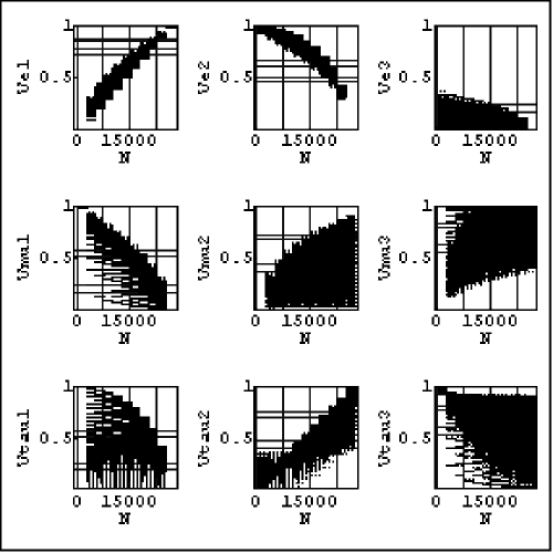
Figure 2: $|V^{MNS}_{ij}|$ for $\tau$ leptogenesis model type I(a) with normal hierarchy and $X_{1}\leq X_{2}$.

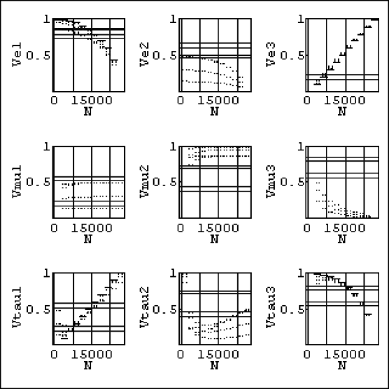
Figure 3: $|V^{MNS}_{ij}|$ for $\tau$ leptogenesis model type I(a) with inverted hierarchy and $X_{1}\leq X_{2}$.

In Fig.3, we show the fit for the inverted heirachical case. By finding $N$ which reproduces the manignitude of five MNS matrix elements simultaneously, we can determine the parameters of the model. In this way, one can find $N$ which puts MNS matrix elements within experimentally allowed range. In table III, we show our fit based on the experimental determination of the mixing angles at $90\%$ CL. Only four types of textures are allowed and all the types correspond to normal hierarchical case and either $\mu$ or $\tau$ leptogenesis case. $|V^{MNS}_{e3}|$ is determined to be non-zero and the upper bound for CP violation $|J|$ is obtained. In table IV, we relax experimental constraints by using $3\sigma$ allowed range. In this case, more textures are allowed and the allowed ranges are larger than previous case. In addition to the previous allowed textures, the type II e-leptogenesis (inverted hierarchical) case are allowed. As for the type I $\mu$ and $\tau$ leptogenesis, the inverted hierachical cases can be also fitted. Let us summarize the fitted results for each texture as follows.

type	$|V^{MNS}_{e1}|$	$|V^{MNS}_{e2}|$	$|V^{MNS}_{e3}|$	$|V^{MNS}_{\mu 3}|$	$|V^{MNS}_{\tau 3}|$	$|J|$
exp. ($90\%$)	$0.79\sim 0.86$	$0.50\sim 0.61$	$0\sim 0.16$	$0.63\sim 0.79$	$0.60\sim 0.77$
I(a) $\mu$ normal $X_{1}\leq X_{2}$	$0.79\sim 0.86$	$0.50\sim 0.61$	$0.058\sim 0.11$	$0.63\sim 0.79$	$0.60\sim 0.77$	$0\sim 0.023$
I(b) $\mu$ normal $X_{2}\leq X_{1}$	$0.79\sim 0.86$	$0.50\sim 0.61$	$0.058\sim 0.11$	$0.64\sim 0.79$	$0.61\sim 0.77$	$0\sim 0.024$
I(a) $\tau$ normal $X_{1}\leq X_{2}$	$0.79\sim 0.86$	$0.50\sim 0.61$	$0.054\sim 0.10$	$0.63\sim 0.79$	$0.61\sim 0.77$	$0\sim 0.022$
I(b) $\tau$ normal $X_{2}\leq X_{1}$	$0.79\sim 0.86$	$0.50\sim 0.61$	$0.054\sim 0.10$	$0.63\sim 0.79$	$0.61\sim 0.77$	$0\sim 0.022$

Table 3: The predictions for $|V^{MNS}_{ij}|$ and $|J|$. The magnitutes of the $V^{MNS}_{ij}$ given in the second row correspond to experimental constraints at $90\%$ CL taken from [12].

type	$|V^{MNS}_{e1}|$	$|V^{MNS}_{e2}|$	$|V^{MNS}_{e3}|$	$|V^{MNS}_{\mu 3}|$	$|V^{MNS}_{\tau 3}|$	$|J|$
exp.($3\sigma$)	$0.73\sim 0.88$	$0.47\sim 0.67$	$0\sim 0.23$	$0.56\sim 0.84$	$0.54\sim 0.82$
I(a) $\mu$ normal $X_{1}\leq X_{2}$	$0.73\sim 0.88$	$0.47\sim 0.67$	$0.046\sim 0.13$	$0.57\sim 0.83$	$0.54\sim 0.82$	$0\sim 0.028$
I(b) $\mu$ normal $X_{2}\leq X_{1}$	$0.73\sim 0.88$	$0.47\sim 0.67$	$0.047\sim 0.13$	$0.57\sim 0.83$	$0.54\sim 0.82$	$0\sim 0.028$
I(a) $\tau$ normal $X_{1}\leq X_{2}$	$0.73\sim 0.88$	$0.47\sim 0.67$	$0.044\sim 0.13$	$0.56\sim 0.84$	$0.54\sim 0.82$	$0\sim 0.027$
I(b) $\tau$ normal $X_{2}\leq X_{1}$	$0.73\sim 0.88$	$0.47\sim 0.67$	$0.043\sim 0.12$	$0.56\sim 0.84$	$0.54\sim 0.82$	$0\sim 0.027$
I(a) $\mu$ inverted $X_{1}\leq X_{2}$	$0.86\sim 0.87$	$0.48\sim 0.49$	$0.027\sim 0.14$	$0.63\sim 0.82$	$0.56\sim 0.77$	$0.0055\sim 0.027$
I(b) $\mu$ inverted $X_{2}\leq X_{1}$	$0.86\sim 0.87$	$0.48\sim 0.49$	$0.022\sim 0.14$	$0.57\sim 0.84$	$0.54\sim 0.82$	$0.0044\sim 0.028$
I(a) $\tau$ inverted $X_{1}\leq X_{2}$	$0.86\sim 0.87$	$0.48\sim 0.49$	$0.027\sim 0.13$	$0.59\sim 0.84$	$0.54\sim 0.80$	$0.0055\sim 0.026$
I(b) $\tau$ inverted $X_{2}\leq X_{1}$	$0.86\sim 0.87$	$0.48\sim 0.49$	$0.021\sim 0.13$	$0.57\sim 0.84$	$0.55\sim 0.82$	$0.0039\sim 0.027$
II(a) e inverted $X_{1}\leq X_{2}$	$0.87$	$0.49\sim 0.50$	$0$	$0.57\sim 0.84$	$0.55\sim 0.82$	$0$
II(b) e inverted $X_{2}\leq X_{1}$	$0.87$	$0.49\sim 0.50$	$0$	$0.57\sim 0.84$	$0.55\sim 0.82$	$0$

Table 4: The predictions for $|V^{MNS}_{ij}|$ and $|J|$. The magnitutes of the $V^{MNS}_{ij}$ given in the second row correspond to experimental constraints at $3\sigma$ taken from [12].

• Type II e-leptogenesis scenarios. In this class of models, because $|V^{MNS}_{e3}|=0$, CP violation in neutrino oscillation $J$ is vanishing in spite of non-zero $\gamma$.

• Type I $\mu$ and $\tau$ leptogenesis for normal hierarchical case. In this class of models, $V^{MNS}_{e3}$ is non-vanishing. About CP violation phase, the allowed range of $|J|$ is from zero to some non-vanishing value.

• Type I $\mu$ and $\tau$ leptogenesis for inverted hierarchical case. In this class of models, both $V^{MNS}_{e3}$ and $|J|$ are non-vanishing.

IV.2 $|V^{MNS}_{e3}|$ versus $|J|$

To clarify the differences of predictions between inverted hierarchical case and normal hierarchical case, we have plotted $|V^{MNS}_{e3}|$ versus $|J|$ in Figs. 4-6. When $|V^{MNS}_{e3}|\ll 1$, $J$ is approximately proportional to $|V^{MNS}_{e3}|$. By choosing the standard parametrization of MNS matrix, we obtain,

$$J=(1-s_{13}^{2})s_{13}c_{12}s_{12}c_{23}s_{23}\sin\delta,$$ (96)

with $V^{MNS}_{e3}=s_{13}\exp(-i\delta)$.

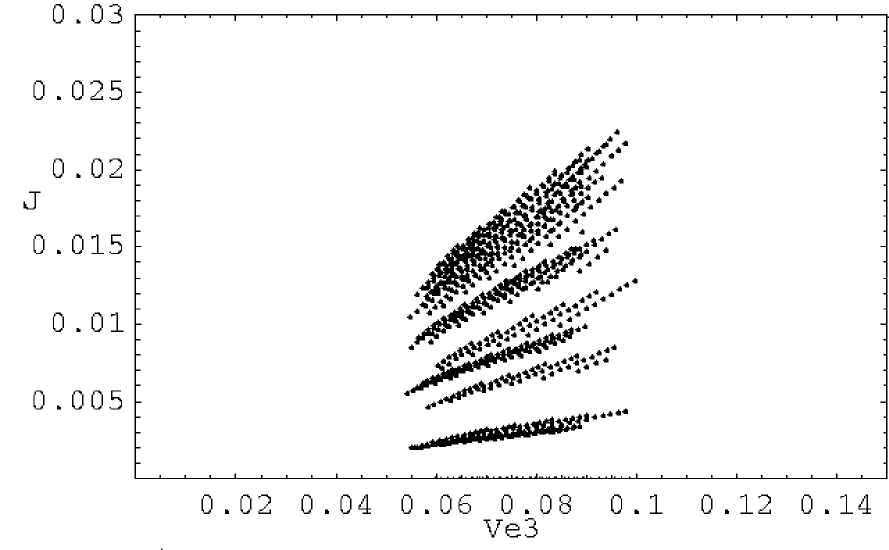
Figure 4: $|J|$ and $|V^{MNS}_{e3}|$ for $\tau$ leptogenesis model type I(a) with normal hierarchy and $X_{1}\leq X_{2}$. ($90\%$)

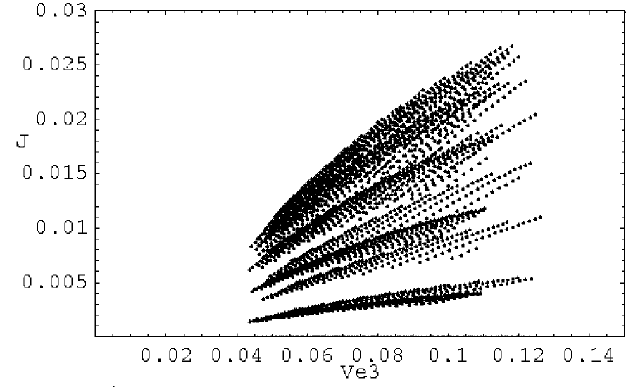
Figure 5: $|J|$ and $|V^{MNS}_{e3}|$ for $\tau$ leptogenesis model type I(a) with normal hierarchy and $X_{1}\leq X_{2}$. ($3\sigma$)

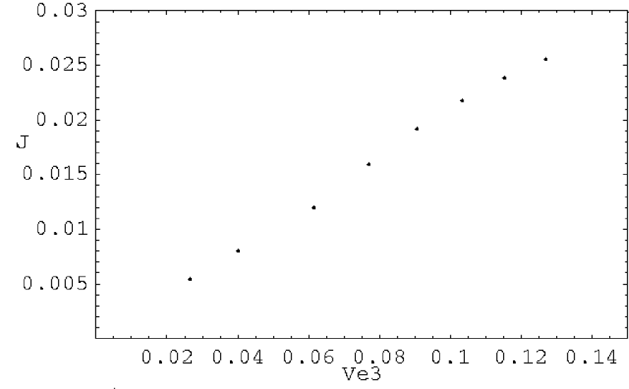
Figure 6: $|J|$ and $|V^{MNS}_{e3}|$ for $\tau$ leptogenesis model type I(a) with inverted hierarchy and $X_{1}\leq X_{2}$.

In Figs. 4-6, within good approximation, we can find the linear correlation between $|J|$ and $|V^{MNS}_{e3}|$. One can read $|\sin\delta|$ from the slope since

$$|\sin\delta|\simeq\frac{1}{c_{12}s_{12}c_{23}s_{23}}\frac{|J|}{s_{13}}.$$ (97)

In type I models with normal hierachy, $\mu-$ and $\tau-$leptogenesis are allowed. The allowed range for $\sin\delta$ is,

$$0\leq|\sin\delta|\lesssim 1.$$ (98)

For type I with inverted hierachy, $\sin\delta$ is almost maximal,

$$|\sin\delta|\simeq 1,$$ (99)

which implies that CP violating phase $\gamma$ takes some non-vanishing definite value. By fitting the data of neutrino mixings, we have determined the allowed ranges for the parameters which are presented in table 5.

Table 5: The parameters which are determined by fitting with mixing angles. The values in parentheses are obtained by fitting with the magnitudes of MNS elements based on $3\sigma$ based fit taken from [12]. The others correspond to $90\%$ CL level fit in [12].

			$|\gamma|$	$\beta$
II(a) $e$ inv. $X_{1}\leq X_{2}$	$(0.30)\leq|u_{\mu 2}|^{2}\leq(0.67)$	$(0.33)\leq|u_{\tau 2}|^{2}\leq(0.70)$	$(1.4)\sim(1.8)$	$(1.5)$
II(b) $e$ inv. $X_{1}\geq X_{2}$	$(0.30)\leq|u_{\mu 1}|^{2}\leq(0.67)$	$(0.33)\leq|u_{\tau 1}|^{2}\leq(0.70)$	$(1.4)\sim(1.8)$	$(1.5)$
I(a) $\mu$ nor. $X_{1}\leq X_{2}$	$0.085\leq|u_{e1}|^{2}\leq 0.29$	$0.24\leq|u_{\tau 2}|^{2}\leq 0.68$	$0\sim 3.1$	$0.60\sim 1.1$
	$(0.050)\leq|u_{e1}|^{2}\leq(0.37)$	$(0.16)\leq|u_{\tau 2}|^{2}\leq(0.75)$	$(0)\sim(3.1)$	$(0.47)\sim(1.1)$
I(a) $\mu$ inv. $X_{1}\leq X_{2}$	$(0.97)\leq|u_{e1}|^{2}\leq(1.0)$	$(0.40)\leq|u_{\tau 2}|^{2}\leq(0.68)$	$(1.4)\sim(1.8)$	$(1.5)$
I(b) $\mu$ nor. $X_{1}\geq X_{2}$	$0.25\leq|u_{\tau 1}|^{2}\leq 0.68$	$0.082\leq|u_{e2}|^{2}\leq 0.29$	$0\sim 3.1$	$0.60\sim 1.1$
	$(0.16)\leq|u_{\tau 1}|^{2}\leq(0.75)$	$(0.050)\leq|u_{e2}|^{2}\leq(0.37)$	$(0)\sim(3.1)$	$(0.47)\sim(1.1)$
I(b) $\mu$ inv.$X_{1}\geq X_{2}$	$(0.33)\leq|u_{\tau 1}|^{2}\leq(0.70)$	$(0.97)\leq|u_{e2}|^{2}\leq(1.0)$	$(1.4)\sim(1.8)$	$(1.5)$
I(a) $\tau$ nor. $X_{1}\leq X_{2}$	$0.093\leq|u_{e1}|^{2}\leq 0.29$	$0.28\leq|u_{\mu 2}|^{2}\leq 0.71$	$0\sim 3.1$	$0.63\sim 1.1$
	$(0.054)\leq|u_{e1}|^{2}\leq(0.38)$	$(0.18)\leq|u_{\mu 2}|^{2}\leq(0.78)$	$(0)\sim(3.1)$	$(0.50)\sim(1.2)$
I(a) $\tau$ inv. $X_{1}\leq X_{2}$	$(0.98)\leq|u_{e1}|^{2}\leq(1.0)$	$(0.30)\leq|u_{\mu 2}|^{2}\leq(0.64)$	$(1.4)\sim(1.8)$	$(1.5)$
I(b) $\tau$ nor. $X_{1}\geq X_{2}$	$0.28\leq|u_{\mu 1}|^{2}\leq 0.71$	$0.092\leq|u_{e2}|^{2}\leq 0.29$	$0\sim 3.1$	$0.63\sim 1.1$
	$(0.18)\leq|u_{\mu 1}|^{2}\leq(0.78)$	$(0.054)\leq|u_{e2}|^{2}\leq(0.37)$	$(0)\sim(3.1)$	$(0.50)\sim(1.2)$
I(b) $\tau$ inv.$X_{1}\geq X_{2}$	$(0.30)\leq|u_{\mu 1}|^{2}\leq(0.67)$	$(0.97)\leq|u_{e2}|^{2}\leq(1.0)$	$(1.4)\sim(1.8)$	$(1.5)$

IV.3 Unitarity triangle

Further one can reconstruct the unitarity triangles of the models with two zeros texture which can satisfy the experimental constraints. We focus on the unitarity triangle of $\mu-e$ sector

$$V^{MNS}_{e1}V^{MNS\ast}_{\mu 1}+V^{MNS}_{e2}V^{MNS\ast}_{\mu 2}+V^{MNS}_{e3}V^{MNS\ast}_{\mu 3}=0,$$

$$V^{MNS}_{e1}V^{MNS\ast}_{\mu 1}=-c_{13}\left(c_{12}s_{12}c_{23}+c_{12}^{2}s_{23}s_{13}\exp(-i\delta)\right),$$

$$V^{MNS}_{e2}V^{MNS\ast}_{\mu 2}=c_{13}\left(s_{12}c_{12}c_{23}-s_{12}^{2}s_{23}s_{13}\exp(-i\delta)\right),$$

$$V^{MNS}_{e3}V^{MNS\ast}_{\mu 3}=+c_{13}s_{13}s_{23}\exp(-i\delta).$$ (100)

First we show the triangle schematically in Fig. 7. The triangle can be drawn inside a parallelogram as shown in Fig. 7. We note that,

$$\rm{OB:AB}=c_{12}^{2}:s_{12}^{2},$$ (101)

and $\delta$ is argument between $V_{e3}^{MNS}$ and real axis.

Figure 7: Schematic view of unitarity triangle

In Fig.8 and in Fig.9, we have shown the triangle corresponding to the type I(a) $\tau$ leptogenesis for normal and inverted hierarchical case, respectively. As we have already noted, the inverted hierachical case, $\sin\delta$ is almost maximal. Therefore the argument of $V_{e3}$ with respect to real axis is 90 degree. For normal hierachical case, $|\sin\delta|$ is smaller than $1$. Because only the magnitude of $V^{MNS}$ is known, we have two fold ambiguities for $\delta$ even if the sizes of $s_{12}$, $s_{23}$, $|V_{e3}^{MNS}|$ and $|J|$ are given. In Fig. 8, we plot two triangles which correspond to $\delta$ and $-\delta$. Two triangles which are related to each other by reflection with respect to real axis can be distinguished by measuring the sign of $J$.

Figure 8: Unitarity triangles for $\tau$ leptogenesis model type I(a) with normal hierarchy which correspond to $|V_{e1}|\simeq 0.80,|V_{e2}|\simeq 0.60,|V_{e3}|\simeq 0.098,|V_{\mu 1}|\simeq 0.41,|V_{\mu 2}|\simeq 0.65,|V_{\mu 3}|\simeq 0.64,|V_{\tau 3}|\simeq 0.76,|J|\simeq 0.0044$, $|\sin\delta|\simeq 0.19$, $|\gamma|\simeq 3.0$ and $\beta\simeq 0.94$.

Figure 9: Unitarity triangles for $\tau$ leptogenesis model type I(a) inverted hierarchy which correspond to $|V_{e1}|\simeq 0.86,|V_{e2}|\simeq 0.49,|V_{e3}|\simeq 0.13,|V_{\mu 1}|\simeq 0.40,|V_{\mu 2}|\simeq 0.70,|V_{\mu 3}|\simeq 0.59,|V_{\tau 3}|\simeq 0.80,|J|\simeq 0.026$, $|\sin\delta|\simeq 1.0,|\gamma|\simeq 1.6$ and $\beta\simeq 1.5$.

V Summary and Discussions

In this work, we study CP violation in neutrino oscillations and its possible connection with lepton family asymmetries generated from heavy Majorana neutrino decays. We have derived a general formula for CP violation in neutrino oscillations in terms of heavy Majorana mass terms and Dirac mass terms. We identify the two zeros texture models in which lepton asymmetry is dominated by a particular family asymmetry. We have explored the e-leptogenesis, $\mu-$leptogenesis and $\tau-$leptogenesis scenarios and determined the allowed range of parameters from the neutrino experimental results. Using the $90\%$ and $3\sigma$ bound on the magnitude of mixing angles measured at experiments, we have constrained the parameters of the models. Based on the analysis above, we have predicted the possible ranges of $|V_{e3}^{MNS}|$ and the low energy CP violation observable $|J|$. We have found that in the models with two zeros in $m_{D}$ and inverted hierarchy, $|\sin\delta|$ is predicted to be almost maximal. Once those two unknown quantities are determined in future neutrino oscillation experiments, we could compare them with our predictions. Because the sign of J would be determined from the measurment of CP violation via neutrino oscillations, we can conclude whether the sign of CP violation at low energy is consistent with CP violation required in cosmology [3] [5] [6].

VI Acknowledgement

We thank Z. Xiong and Z. Xing for discussions. We also thank the Yukawa Institute for Theoretical Physics at Kyoto University, where this work was initiated during the workshop YITP-W-04-08 on $``$Summer Institute 2004” and YITP-W-04-21 on $``$CP violatioin and matter and anti-matter asymmetry”. This work is supported by the kakenhi of MEXT, Japan, No. 16028213(T.M.). SKK is supported in part by BK21 program of the Ministry of Education in Korea and in part by KOSEF Grant No. R01-2003-000-10229-0.

References

- [1] M. Fukugita and T. Yanagida, Phys. Lett. B174, 45 (1986).
- [2] T. Endoh, T. Morozumi, A. Purwanto and T. Onogi, Phys. Rev. D64, 013006 (2001), Erratum-ibid.D64:059904,2001.
- [3] G.C. Branco, T. Morozumi, B. Nobre, and M. N. Rebelo, Nucl. Phys. B617, 475 (2001).
- [4] T. Endoh, T. Morozumi, and Z. Xiong, Prog. Theor. Phys. 111, 123 (2004).
- [5] P.H. Frampton, S.L. Glashow, and T. Yanagida, Phys. Lett. B548, 119 (2002).
- [6] T. Endoh, S. Kaneko, S.K. Kang, T. Morozumi, and M. Tanimoto, Phys. Rev. Lett. 89, 231601 (2002).
- [7] W. Guo and Z. Xing, Phys. Lett. B583, 163 (2004).
- [8] J. Mei and Z. Xing, Phys. Rev. D69, 013006 (2000).
- [9] L. Covi, E. Roulet, and F. Vissani, Phys. Lett. B384, 169 (1996).
- [10] C. Jarlskog, Phys. Rev. Lett. 55, 1039 (1985).
- [11] M. Fukugita and M. Tanimoto, Phys. Lett. B515, 30 (2001).
- [12] M.C. Gonzalez-Garcia and C. Pena-Garay, Phys. Rev. D68, 093003 (2003).