Collider phenomenology of Higgs bosons in Left-Right symmetric Randall-Sundrum models

Abstract:

We investigate the collider phenomenology of a left-right symmetric Randall-Sundrum model with fermions and gauge bosons in the bulk. We find that the model is allowed by precision electroweak data as long as the ratio of the (unwarped) Higgs vev to the curvature scale is $v/k\leq 1/4$. In that region there can be substantial modifications to the Higgs properties. In particular, the couplings to $WW$ and $ZZ$ are reduced, the coupling to gluons is enhanced, and the coupling to $\gamma\gamma$ can receive shifts in either direction. The Higgs mass bound from LEP II data can potentially be relaxed to $m_{H}\gtrsim 80$ GeV.

1 Introduction

While the Standard Model (SM) is a spectacularly successful description of high energy particle phenomena, it leaves unexplained why the Electroweak scale is much smaller than the GUT or Planck scales. Recently, it has been proposed that this hierarchy might be explained by the presence of additional compactified dimensions. These could be TeV scale and flat [1, 2], or Planck scale with a warped geometry [3]. In this second scenario, the Randall-Sundrum (RS) model, there is a single extra dimension and the spacetime has the geometry of five-dimensional Anti-de Sitter space, $AdS_{5}$, compactified on an orbifolded circle, $S^{1}/Z_{2}$. One 3-brane is localized on each end of the orbifold, and the warping between them generates the Electroweak scale.

In the original RS model, all SM fields are localized on the TeV (or IR) brane. The observable phenomenology in this case comes from the new spin-2 graviton resonances [4]. However, there is no reason for the fermions and gauge fields not to propagate in the bulk [5, 6, 7, 8]. Indeed, bulk fermions have a zero mode which is exponentially localized near one of the branes. Choosing ${\mathcal{O}}(1)$ Lagrangian parameters for different fermions can select exponentially different overlaps on the IR brane, and hence different masses, providing a possible explanation of the fermion mass hierarchy [7, 9, 10]. There have been many investigations into the phenomenology of this model [11, 12, 13, 14, 15]. One important conclusion is that simply putting the SM gauge group in the bulk produces a large Peskin-Takeuchi $T$-parameter [16]. The can be fixed by expanding the gauge group to be left-right symmetric, $SU(2)_{L}\times SU(2)_{R}\times U(1)_{B-L}$ [17] or by introducing brane localized kinetic terms for the fermions [18]. It is also possible to extend this to a Grand Unified group which then contains a dark matter candidate [19, 20].

More recently, there has been a proposal that no Higgs is needed in this model, as the geometry can set the gauge boson masses [21, 22, 23], as well as the fermion masses [24]. The most straightforward application of this model produces large electroweak corrections, and does not preserve tree-level unitarity in longitudinal gauge boson scattering at finite center-of-mass scattering energies [25, 26, 27, 28, 29, 30, 31, 32, 33]. They do, however, contain a rich collider phenomenology which is largely independent of those considerations [34]. There have been several variations on the model, including deconstructing the extra dimension [35, 36, 37, 38, 39, 40, 41], adding additional dimensions [42], and adding additional branes [43].

The Higgsless models can be obtained as the limit of a model with a Higgs where the vev, $v$, is taken to be large compared to the $AdS$ curvature $k$; that is $v/k\gg 1$. The fact that Higgsless scenarios have difficulty accommodating the precision electroweak observables leads to the speculation that the agreement may be improved by including the effects of a finite Higgs vev.

Additionally, analysis of the Higgs scenario, $v/k\ll 1$ show that this model is allowed by precision electroweak data. However, in this case, with Kaluza-Klein (KK) masses, $m_{KK}\approx 2-3{\ \rm TeV}$, we have $v/k\approx 1/4$, which is not particularly small. In fact, this is expected from RS effective field theory arguments which tell us that all Lagrangian level mass parameters should be of the same order, $M_{\rm Pl}$. Hence, it makes sense to study the corrections to collider observables induced by a finite, but not large, Higgs vev.

In this paper we will examine the numerical behavior of explicit solutions for the gauge and fermion wavefunctions in RS with a finite and arbitrary value for $v/k$. From this we can extract both the small vev limit and the Higgsless limit.

Note that the RS models can be thought of as large $N$ 4D conformal gauge theories through the $AdS/CFT$ correspondence [44]. Analyses have also been performed on the CFT side of the Higgsless model [45], and the Higgs model [46, 47]. Note also that there is potentially a term that mixes the Higgs field with the scalar curvature, inducing mixing between the Higgs and radion states [48, 49]. However, the coefficient of this term can be set to zero, which we will do here.

In Section 2 we develop the formalism that will be employed in this paper. Section 3 shows the behavior of the Kaluza-Klein spectra as the Higgs vev is varied. We investigate the gauge couplings and precision electroweak constraints in Section 4, and the corrections to Higgs properties in Section 5. Section 6 concludes.

2 Formalism

We work in a slice of $AdS_{5}$, with metric (in conformal coordinates)

$$ds^{2}=\left(\frac{R}{z}\right)^{2}(dx^{2}-dz^{2})$$ (1)

where $R=1/k$ is the inverse of the curvature scale. There is one brane located at $z=R$ (the Planck or UV brane), and a second brane at $R^{\prime}=(M_{\rm Pl}/TeV)R$ (the TeV or IR brane). This gives $\log(R^{\prime}/R)\sim 35$. We define $\epsilon=R/R^{\prime}\sim 10^{-15}$ for later convenience.

We are interested in models with a bulk $SU(2)_{L}\times SU(2)_{R}\times U(1)_{B-L}$ gauge symmetry. The additional $SU(2)_{R}$ factor over the SM provides a bulk custodial $SU(2)_{\rm c}$, which can successfully protect the $T$ parameter [17]. The bulk gauge action we consider is then

$$S_{bulk}=\int d^{5}x\sqrt{g}\left(\frac{-1}{4g^{2}_{5L}}F^{L}_{MN}F^{MN}_{L}+\frac{-1}{4g^{2}_{5R}}F^{R}_{MN}F^{MN}_{R}+\frac{-1}{4g^{2}_{5B}}F^{B}_{MN}F^{MN}_{B}\right)$$ (2)

(Note that there is also a term for the gluon fields, which must also be bulk fields. However, this term is unimportant for this paper). We will make use of the ratios of gauge couplings

$$\kappa=g_{5R}/g_{5L},\qquad\lambda=g_{5B}/g_{5L}.$$ (3)

Clearly, this group needs to be broken to $U(1)_{\rm EM}$. We accomplish this by separating the breaking into two sectors. On the Planck brane we break $SU(2)_{R}\times U(1)_{B-L}\rightarrow U(1)_{Y}$. Since the UV brane is the only place where the $SU(2)_{\rm c}$ is broken, we can see why the effects on the $T$ parameter will be small. On the TeV brane we break $SU(2)_{L}\times SU(2)_{R}\rightarrow SU(2)_{D}$, where $SU(2)_{D}$ is the diagonal subgroup of $SU(2)_{L}$ and $SU(2)_{R}$.

We will work in the $A^{5}=0$ (unitary) gauge. The gauge condition can potentially be complicated by the fact that the brane localized Goldstone modes, the $G^{i}$ can mix with the $A^{5}$ modes. This means that the physical longitudinal polarization for each vector is a combination of bulk and brane modes. However, for the breaking pattern used here there is no zero mode for any of the $A^{5}$ fields, and hence no extra physical zero-mode scalar. We can therefore safely work in the gauge where $A^{5}=G^{i}=0$.

We now ask what drives the breaking on each brane. On the Planck brane all degrees of freedom will have Planck scale masses, so we can ignore them. We can then implement the breaking with boundary conditions to good approximation. This leads to the boundary conditions at $z=R$

$$\partial_{z}\left(\frac{\kappa}{\lambda}A_{R}-A_{B}\right) =0, \partial_{z}A_{L} =0,\hfill$$

$$A_{B}-\frac{\kappa}{\lambda}A_{R}^{3} =0, A_{R}^{\pm} =0.$$ (4)

On the TeV brane, the masses will be TeV scale, so we should look at the Higgs sector in detail. The simplest structure that will create the breaking pattern is a real Higgs that is a bidoublet under $SU(2)_{L}\times SU(2)_{R}$. This leads to the boundary conditions at $z=R^{\prime}$

$$\partial_{z}(A_{L}+\kappa A_{R}) =0, \partial_{z}A_{B}=0,\hfill$$

$$\partial_{z}(\kappa A_{L}-A_{R}) =-\frac{g^{2}_{5L}v^{2}}{4}(\kappa A_{L}-A_{R}).$$ (5)

Note that in the $v/k\to\infty$ limit we obtain the usual Higgsless boundary conditions. Instead of the real bidoublet, we could also use the complex bidoublet familiar from Left-Right symmetric models with minimal changes. See Appendix A for details.

To write down the effective 4D theory we expand the 5D fields into Kaluza Klein (KK) fields.

$$A(x,z)=\sum_{n}\zeta^{(n)}_{A}(z)A^{(n)}(x)$$ (6)

We can now obtain the gauge boson wavefunctions by solving the equation of motion subject to the boundary conditions (4) and (5). The generic solution for the wavefunctions is

$$\zeta_{A}^{(n)}(z)=z(A_{A}^{(n)}J_{1}(m_{n}z)+B_{A}^{(n)}Y_{1}(m_{n}z)).$$ (7)

Here the label $A$ refers to the particular gauge field being expanded. One of the coefficients, $A^{(n)}$ and $B^{(n)}$, and the mass are determined by inserting eq. (7) into eqs. (4) and (5). The other coefficient is fixed by the normalization condition. We will use 4D canonical normalization for all fields, giving

$$N_{W}^{(n)2}=\int_{R}^{R^{\prime}}\frac{dz}{z}R\left(|\zeta^{(n)}_{A^{\pm}_{L}}(z)|^{2}+|\zeta^{(n)}_{A^{\pm}_{R}}(z)|^{2}\right),$$ (8)

for the charged gauge bosons, and

$$N_{Z}^{(n)2}=\int_{R}^{R^{\prime}}\frac{dz}{z}R\left(|\zeta^{(n)}_{A^{0}_{L}}(z)|^{2}+|\zeta^{(n)}_{A^{0}_{R}}(z)|^{2}+|\zeta^{(n)}_{B_{R}}(z)|^{2}\right),$$ (9)

for the neutral tower.

The fermion sector of the theory is more intricate. First, we will need to arrange the SM fermions into representations of $SU(2)_{R}$. There are two ways to do this in the RS model. The most straightforward is to pair corresponding $SU(2)_{L}$ singlets into a single $SU(2)_{R}$ doublet. So, e.g $u_{R}$ and $d_{R}$ become $\begin{pmatrix}u_{R}&d_{R}\end{pmatrix}^{\top}$. The other option is to make each right-handed field part of a different $SU(2)_{R}$ doublet. So $u_{R}\to\begin{pmatrix}u_{R}&d^{\prime}_{R}\end{pmatrix}^{\top}$, etc.. Orbifold projections are then required to insure that there is no light mode for the new fermion states. The first option follows more naturally from Grand Unified theories, and allows the possibility of an explicit $Z_{2}$ symmetry that exchanges the Left and Right gauge groups. The second makes it easier to obtain top-bottom splitting and to suppress corrections to the $Zb\bar{b}$ vertex, and is compatible with the GUT scenario in [20]. Here we will study the case where there is an explicit $Z_{2}$, and hence choose to combine right-handed fields into a single $SU(2)_{R}$ multiplet.

We write the 5D fermion as two 4D Majorana fermions, $\Psi_{i}=(\psi_{i}\ \chi_{i})^{\top}$. The orbifold conditions tell us that one component must be even and the other odd [6]. We will pick the $\psi_{i}$ to be even for fields corresponding to the left-hand SM fermions, and the $\chi_{i}$ even for the right-handed ones. The Yukawa couplings to $\phi$, the Higgs on the IR brane, will connect the left and right-handed zero modes and lift them. These couplings are

$$S_{IR}=\sum_{f}\int d^{4}x\left(\frac{R}{z}\right)^{4}\lambda_{f}\phi\left(\psi^{f}_{Ri}\chi^{f}_{Li}+\bar{\chi}^{f}_{Li}\bar{\psi}^{f}_{Ri}+\psi^{f}_{Li}\chi^{f}_{Ri}+\bar{\chi}^{f}_{Ri}\bar{\psi}^{f}_{Li}\right).$$ (10)

Here $f$ labels the fermion flavor. Eq. (10) induces the boundary conditions at $z=R^{\prime}$

$$\psi^{f}_{L}=-\lambda_{f}v\psi^{f}_{R}\qquad\chi^{f}_{R}=\lambda_{f}v\chi^{f}_{L}.$$ (11)

This is equivalent to introducing a Dirac mass $\lambda_{f}v$ on the IR brane. Note that this is $SU(2)_{D}$ symmetric, and hence can not generate different masses for the up and down-type quarks. That splitting must be generated on the UV brane, which is the only place where the custodial symmetry is broken. It was demonstrated in [24] that the simplest way to do this with a complex fermion is to introduce brane-localized fermions that can mix with the bulk states. So we include a contribution to the brane action for each SM right-handed fermion

$$S_{\rm UV}=\int d^{4}x\sum_{f}\left(-i\bar{\xi}^{f}\bar{\sigma}^{\mu}\partial_{\mu}\xi^{f}-i\eta^{f}\bar{\sigma}^{\mu}\partial_{\mu}\bar{\eta}^{f}+F(\eta^{f}\xi^{f}+\bar{\eta}^{f}\bar{\xi}^{f})+M_{f}R^{1/2}(\psi^{f}_{R}\xi+\bar{\xi}\bar{\psi}^{f}_{R})_{z=R}\right)$$ (12)

where $\xi_{i}$ and $\eta_{i}$ are the brane localized states, $\psi_{Ri}$ is the component of the bulk state that has a zero mode, and the index $f$ runs over all SM right-handed fermions. This leads to the boundary condition

$$\psi^{f}_{L}=0\qquad\chi^{f}_{R}=m_{n}M^{f2}_{m}/F^{2}\psi^{f}_{R}.$$ (13)

The fermion KK expansion will take the form

$$\chi=\sum_{n}g^{(n)}(z)z^{3/2}\chi^{(n)}(x),\qquad\bar{\psi}=\sum_{n}f^{(n)}(z)z^{3/2}\bar{\psi}^{(n)}(x).$$ (14)

Again, we will normalize these canonically, giving

$$\int\frac{dz}{z}\chi^{(n)*}(z)\chi^{(m)}(z)=\delta_{nm},$$ (15)

and similarly for the $\psi^{(n)}$. Note that 5D fermions are achiral, so we can always write down a mass term in the bulk

$$m_{5}^{f}\bar{\Psi}\Psi\equiv c^{f}k\bar{\Psi}_{f}\Psi_{f}.$$ (16)

Note that the mass itself must be $Z_{2}$-odd, since $\bar{\Psi}\Psi$ is. Even in the presence of this mass term there is still a 4D zero mode for the orbifold even components of $\Psi$ when $v=0$. The $c^{f}$ determine the shape of the wavefunction in the extra dimension. This would-be zero mode wavefunction is

$$f_{f}^{(0)}(z)=A_{f}^{(0)}\left(\frac{z}{R}\right)^{c^{f}-1/2}$$ (17)

We can see that for $c>1/2$ the zero mode is localized to the Planck brane, and for $c<1/2$ it is localized to the TeV brane.

3 Kaluza-Klein spectra

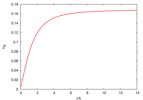
Figure 1: Behavior of the first charged boson mass (corresponding to the observed $W$) as a function of v/k at fixed k. The linear behavior at small $v/k$ corresponds to the ordinary Higgsed model limit, and the flat behavior as $v/k\to\infty$ to the Higgsless limit.

We can solve Eq. (7) subject to (4) and (5) to obtain $x_{W}^{(n)}\equiv m_{W}^{(n)}/k\epsilon$. Figure 1 shows the behavior of $x_{W}^{(1)}$ as a function of $v/k$. Demanding that $m_{W}^{(1)}=m_{W}$ sets the mass scale $k\epsilon$. In the region with $v/k$ small we have $x_{W}^{(1)}\approx\frac{g}{2}\frac{v}{k}$ giving the standard result $k\epsilon\approx\frac{2}{g}m_{W}\frac{k}{v}$. This reflects the fact that as $v/k$ gets small, the KK scale gets large. When $v/k$ is large, $x_{W}^{(1)}$ asymptotes to the Higgsless value $x_{W}^{(1)2}=1/\log(R^{\prime}/R)$ [22].

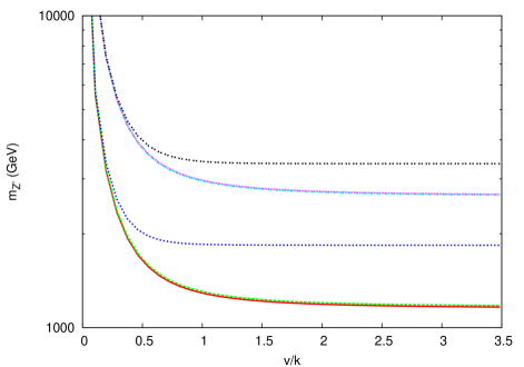
Figure 2: Masses of the first six neutral boson KK excitations lying above the SM $Z$ as a function of $v/k$ with the $W$ and $Z$ masses held fixed at their physical values.

Once this scale has been set, we can solve for the rest of the KK gauge boson masses. For the neutral sector this depends on the additional parameter, $\lambda$. We can solve Eq (7) for the neutral gauge sector for $\lambda$ in terms of $x_{Z}^{(1)}$, the mass of the observed $Z$ boson. We will use this to choose $\lambda$, and hence with our choice of input parameters the on-shell definition of the weak mixing angle, $\sin^{2}\theta_{\rm os}\equiv 1-m_{W}^{2}/m_{Z}^{2}$, is automatically set to the experimental value $\sin^{2}\theta_{\rm os}=0.222$ [50]. These inputs completely determine the gauge KK mass spectrum. Figure 2 shows this spectrum for neutral bosons. Note that each KK level in the $v/k$ small region starts as a degenerate triplet and splits into the doublet-singlet structure seen in Higgsless theories as $v/k$ gets large. These masses are large enough that these states are not bounded by direct detection constraints at the Tevatron[51]. Also, the couplings to light fermions are small enough that they also avoid the LEP II contact interaction constraints [29].

The fermion masses depend on both the brane localized Yukawa couplings to the Higgs and the bulk masses. Eq. (11) shows that the Yukawa couplings provide an effective Dirac mass on the IR brane, and it is this mass that controls the lowest fermion mass (i.e. the mass of the observed SM particle). Hence, the relevant dimensionless parameter is $\lambda_{i}v/k$ (where $\lambda_{i}$ is the relevant Yukawa coupling), rather than $v/k$. In this paper we consider the case where the fermion mass hierarchy generated by the different bulk masses, and not the Yukawas. To correctly produce the top mass, the top/bottom Yukawa must be order 1. We will assume that the other generations have universal Yukawa couplings $\lambda_{\rm light}$. Since we are assuming an explicit $Z_{2}$ symmetry that exchanges the $SU(2)_{L}$ and $SU(2)_{R}$ we have $c^{f}_{L}=-c^{f}_{R}\equiv c^{f}$ (the minus sign arises from the choice of orbifold parities). We will pick the parameters $c^{f}$ to produce the correct fermion masses for a given Yukawa coupling and Higgs vev. In the quark sector we pick the $c^{f}$ to match the up-type masses. We then introduce mixing with $UV$ brane fermions as in Eq. (12) to generate the up-down splitting. In the lepton sector we simply match the charged lepton masses by picking the $c^{f}$, and leave the neutrinos massless. We can then solve for the KK masses, shown in Fig. 3. Note that a large Dirac mass on the IR brane makes the first KK excitation light. This behavior corresponds to that seen in [20]. To avoid light KK leptons we will need $y_{\rm light}\lesssim 1/2$. The values of the $c^{f}$ depend on the value of $v/k$, but not strongly. As an example point, at $v/k\sim 1/10$ we have $c^{t}=0.43$, $c^{c}=0.53$, $c^{u}=0.63$, $c^{\tau}=0.52$, $c^{\mu}=0.58$, and $c^{e}=0.66$. In the Higgsless regime these are all shifted up by about $0.03$.

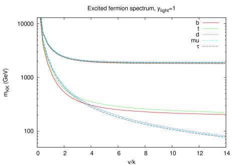
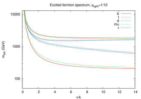
Figure 3: Masses of the first two excited KK fermions as a function of $v/k$ for several species. Note that the mass of the first excitation depends strongly on the IR-brane mass term, but the second excitation does not.

4 Gauge-fermion couplings

Here we will examine how the shifts in couplings of the $W$ and $Z$ to fermions depend on the Higgs vev. The 5D covariant derivative acting on a fermion $\psi$ is (suppressing Lorentz indices)

$$D\psi=\left(\partial_{M}+\int_{R}^{R^{\prime}}\frac{dz}{z}g_{5L}\left(A_{L\mu}T_{L}+\kappa A_{R\mu}T_{R}+\lambda Q_{B-L}A_{B\mu}\right)\right)\psi$$ (18)

with $Q_{B-L}=(B-L)/2$. The electromagnetic charge is $Q=T^{3}_{L}+T^{3}_{R}+Q_{B-L}$. We can rewrite the pieces of $D$ corresponding to the neutral gauge boson couplings as

$$g_{5L}(I^{f}_{3L}-\lambda I^{f}_{B})\left(T^{3}_{L}+\frac{\kappa I^{f}_{3R}-\lambda I^{f}_{B}}{I^{f}_{3L}-\lambda I^{f}_{B}}T^{3}_{R}+\frac{\lambda I^{f}_{B}}{I^{f}_{3L}-\lambda I^{f}_{B}}Q\right).$$ (19)

Where the $I^{f}_{i}=\int_{R}^{R^{\prime}}dz/z\,\zeta_{i}\bar{\psi}_{f}\psi_{f}$ encode the extra dimensional physics. This can be matched onto the covariant derivative from the effective 4D theory

$$g_{Z_{1}f\bar{f}}(T^{3}_{L}+\sin^{2}\theta_{R,f}T^{3}_{R}-\sin^{2}\theta_{\rm eff,f}Q).$$ (20)

This identifies the strength of the $Z$ coupling to fermion $f$ as $g_{Z_{1}f\bar{f}}=g_{5L}(I^{3}_{L}-\lambda I_{B})$, the effective weak mixing angle for that coupling $\sin^{2}\theta_{\rm eff,f}=-\lambda I_{B}/(I^{3}_{L}-\lambda I_{B})$, and a new quantity that measures the strength of the right-handed couplings: $\sin^{2}\theta_{R,f}=(\kappa I^{3}_{R}-\lambda I_{B})/(T^{3}_{L}-\lambda I_{B})$. We can also write an expression similar to Eq. (19) for the charged sector

$$g_{5L}I^{f}_{\pm L}\left(T^{\pm}_{L}+\frac{\kappa I^{f}_{\pm R}}{I^{f}_{\pm L}}T^{\pm}_{R}\right),$$ (21)

giving the strength of the left and right handed couplings.

Note that the wavefunctions for all electroweak particles, with the single exception of the zero mode photon, have non-trivial dependence on the extra dimension. In particular the different flavors of fermions will have different wavefunctions that can be probed by the $W$ and $Z$. Hence, all quantities defined above will depend on the fermion species, as indicated by the label $f$.

Since the photon wavefunction is flat in the extra dimension, the electromagnetic coupling is simply given by (using the normalization from Eq. (9))

$$e^{2}=\frac{g_{5L}^{2}}{R\log(R^{\prime}/R)}\frac{\kappa^{2}\lambda^{2}}{\kappa^{2}+\lambda^{2}+\kappa^{2}\lambda^{2}}.$$ (22)

We can use this to define the 5D coupling in terms of the fine structure constant $\alpha$ by

$$\frac{g_{5L}^{2}}{R}=4\pi\alpha\log(R^{\prime}/R)\left(1+\frac{1}{\lambda^{2}}+\frac{1}{\kappa^{2}}\right).$$ (23)

The advantage of this definition is that it is the only coupling that is independent of the fermion species, and allows us to relate $g_{5L}$ to the measured quantity $\alpha$ without ambiguity.

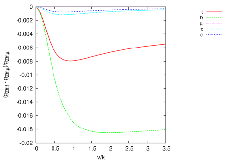
Figure 4: Shifts in the coupling of fermions to the $Z$ induced by the $Z$ wavefunction distortions. The large shift to the $Zb\bar{b}$ coupling is the dominant constraint on $v/k$.

With these definitions we can find the shifts in the couplings. Fig 4 shows the shift in $g_{Zf\bar{f}}$ as a function of $v/k$. Note that the shifts are only large for the third generation quarks. This is expected since they are the only fermions with substantial overlap on the IR brane where the $W$ and $Z$ wavefunctions are distorted. The difference in effects between the top and bottom is due to the $SU(2)_{R}$ violating mixings on the Planck brane, which separately distort the $t$ and $b$ wavefunctions. Imposing the LEP and SLD bound on the shift in the $Zb\bar{b}$ vertex of $\sim 1\%$ [50], we find that $v/k<1/2$. This gives $k\epsilon>800{\ \rm GeV}$, and $v\epsilon<400{\ \rm GeV}$, and hence KK masses of roughly $2$ TeV. This constraint is weaker than that quoted in [17]. The discrepancy can be traced to the different values of $c^{t}$ used, which is due to the allowance here of a larger Lagrangian level Yukawa coupling ($\sim 5$), near the purturbativity bound (that the 4D coupling not exceed $4\pi$). If we reduce the top Yukawa coupling and $c^{t}$ to that in [17], the bound from the $Zb\bar{b}$ coupling would shift to about $v/k\leq 1/4$, corresponding to a KK mass $\sim 4$ TeV, in agreement with [17]. It turns out that the only Higgs properties that follow that is affected by this difference are the corrections to $gg\rightarrow h$ and $h\rightarrow\gamma\gamma$. Since they only depend on this difference at the $20\%$ level, this point is not crucial, and one could simply adopt the stronger bound.

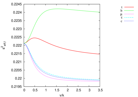
Figure 5: Corrections to the effective weak mixing angle for couplings of fermions to the $Z$ on the $Z$-pole.

In Fig. 5 we see the shifts in the effective weak mixing angle in $Z$-pole observables relative to the on-shell value. The experimental error on this measurement is $\pm 0.00036$ [50], so for $v/k\leq 1/4$ the model shifts correspond to a $2\sigma$ deviation.

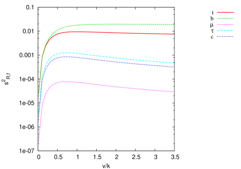
Figure 6: The effective size of the right-handed currents induced by the $SU(2)_{R}$ gauge bosons.

Fig. 6 shows $\sin^{2}\theta_{R}$, the magnitude of the right handed couplings to SM fermions relative to the left handed coupling. Note that the boundary conditions in Eq. 4 cause this to vanish for Planck brane localized fermions. Indeed we see that the closer the fermion to the UV brane, the smaller the effect. In all cases, however, the effect is unobservable in the allowed region $v/k\leq 1/4$.

5 Higgs couplings

We now investigate the shifts in couplings of particles to the physical Higgs boson. As shown above, the main effects come from distortions of the gauge wavefunctions near the IR brane. Schematically, the coupling of a Higgs to two bulk modes will simply be the product of the bulk wavefunctions evaluated at the IR brane, times a Lagrangian parameter. So for the coupling to gauge bosons we have

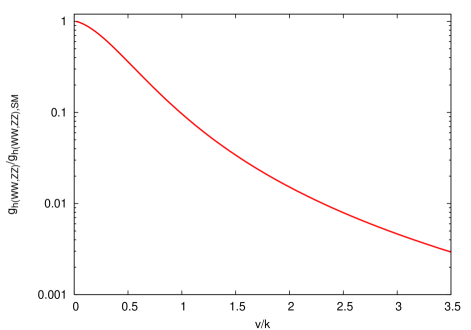
Figure 7: Coupling of the Higgs to vector boson pairs compared to the SM value as a function of $v/k$. Again, the $W$ and $Z$ coupling strengths are nearly identical due to the custodial symmetry.

$$g_{hWW}=\frac{g_{5L}v}{2m_{W}}\frac{1}{1+\kappa^{2}}\left(\zeta^{(1)}_{A^{\pm}_{L}}(R^{\prime})-\kappa\zeta^{(1)}_{A^{\pm}_{R}}(R^{\prime})\right)^{2},$$ (24)

and

$$g_{hZZ}=\frac{g_{5L}v}{2m_{Z}}\frac{1}{1+\kappa^{2}}\left(\zeta^{(1)}_{A^{3}_{L}}(R^{\prime})-\kappa\zeta^{(1)}_{A^{3}_{R}}(R^{\prime})\right)^{2}.$$ (25)

The wavefunction suppression near the TeV brane will decrease these couplings, with $g_{h(WW,ZZ)}\to 0$ as $v/k\to\infty$. This coupling is shown in Fig. 7. This reduction will weaken the LEP bound on the Higgs mass [52]. For $v/k\leq 1/4$ the constraint is relaxed only a few GeV. However, the bound is moves rapidly after that point, so for $v/k=1/2$ the bound is $80{\ \rm GeV}$.

Using the above relations we can find the width for the decay into vector pairs, which is simply

$$\Gamma(h\rightarrow(WW,ZZ))=\left(\frac{1}{2}\right)\frac{g^{2}_{h(WW,ZZ)}m_{(W,Z)}^{3}}{64\pi m_{h}^{2}}(\xi-4)^{1/2}(12-4\xi+\xi^{2}),$$ (26)

with $\xi=m_{h}^{2}/m_{W,Z}^{2}$, and the first factor of $1/2$ is a symmetry factor relevant only for the $ZZ$ final state.

The decay modes where one vector is off-shell can also be important [53]. These decay widths are

$$\Gamma(h\rightarrow WW^{*}) =\frac{3g^{2}_{hWW}g^{2}m_{H}}{512\pi^{3}}H_{W}(m_{W}/m_{H}),$$ (27)

$$\Gamma(h\rightarrow ZZ^{*}) =\frac{g^{2}_{hZZ}g^{2}m_{H}}{2048\pi^{3}\cos^{4}\theta}\left(7-\frac{40}{3}\sin^{2}\theta_{W}+\frac{160}{9}\sin^{4}\theta_{W}\right)H_{Z}(m_{Z}/m_{H}),$$ (28)

where

$$H_{W,Z}(x)=\int_{2x}^{1+x^{2}}dy\frac{(y^{2}-4x^{2})^{1/2}}{(1-y^{2})^{2}+x^{4}\Gamma^{2}_{W,Z}/M_{W,Z}^{2}}(y^{2}-12x^{2}y+8x^{2}+12x^{4}),$$ (29)

and we have ignored the corrections to the $Wf\bar{b}$ and $Zf\bar{f}$ couplings which are small for $v/k\leq 1/4$. It is necessary to include the effects of the finite widths, $\Gamma_{W,Z}$, to match onto Eq. (26).

The fermion couplings to the Higgs are similar; they take the form of the fermion wavefunctions evaluated on the TeV brane times a Yukawa coupling. Specifically,

$$\lambda_{f,n}=\lambda_{f}\left(\chi^{f(n)}_{L}(R^{\prime})\psi^{f(n)}_{R}(R^{\prime})-\psi^{f(n)}_{L}(R^{\prime})\chi^{f(n)}_{R}(R^{\prime})\right).$$ (30)

Note that, since the Kaluza-Klein excitations are localized near the TeV brane, this coupling will be enhanced by the factor $\sqrt{\log(R^{\prime}/R)}$. In the case of the 3rd generation quarks, which have ${\mathcal{O}}(1)$ Lagrangian level Yukawa couplings, these enhancements make the couplings quite large, though in all cases they are less than $4\pi$, and hence perturbative. (Of course, with large couplings the higher order effects are likely to be important, but for the purposes of this paper the rough size indicated by the tree-level result is sufficient). The width into fermion pairs is simply

$$\Gamma(h\to f\bar{f})=\frac{N_{c}\lambda^{2}_{f,1}m_{h}}{32\pi}\left(1-\frac{4m_{f}^{2}}{m_{h}^{2}}\right)^{3/2},$$ (31)

where $N_{c}$ counts the fermion’s color degrees of freedom.

Finally, two of the most important couplings for the discovery of the Higgs boson at the LHC are the Higgs-glue-glue, and Higgs-gamma-gamma vertices. These couplings are absent at tree-level, but are generated radiatively by loops containing fermions and $W$-bosons. In the present model, these vertices receive corrections from two sources. First, the KK excitations of all fermion species can run in the loop (along with the $W$ KK excitations in the case of the $\gamma\gamma$ couplings); since these have substantial couplings to the Higgs these corrections can be large. Second, the suppression in $g_{HWW}$ from the distortion of the $W$ wavefunction can suppress the coupling of the Higgs to two photons. We can calculate in the effective 4D theory obtained by doing the Kaluza-Klein reduction. After doing this, all of the information about the extra dimensional physics is contained in the masses and couplings of the KK states. Hence, to calculate these contributions, we can adapt the formulae from [54] (see also [55]), which computed these shifts in the context of Universal Extra Dimensions, by simply replacing the masses and couplings.

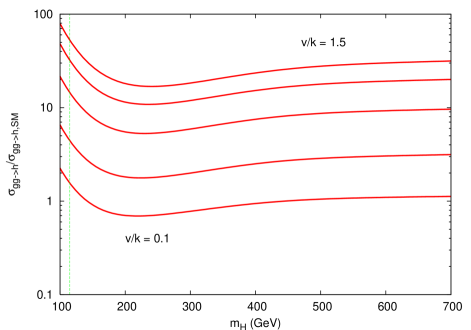
Figure 8: Ratio (at lowest order) of the production cross section for $gg\to h$ compared with the value in the SM. The different curves correspond to the values of $v/k$ from top to bottom of (1.5, 1.1, 0.8, 0.4, 0.1). Here we have taken $y_{\rm light}=1/10$.

The parton level cross section for producing a Higgs from gluon fusion is

$$\sigma_{gg\to h}=\frac{G_{F}[\alpha_{s}(m_{H})]^{2}}{32\sqrt{2}\pi m_{H}^{4}}\left|\sum_{i}F^{i}\right|^{2}.$$ (32)

Here the sum runs over all KK states (including the zero modes) of all colored fermions, with $i$ labeling the flavor. The kinematic function $F^{i}$ is

$$F^{i}=2m_{i}\sum_{n}m_{i,n}\lambda_{i,n}\{-2+(m_{H}^{2}-4m_{i,n}^{2})C_{0}(m_{i,n})\},$$ (33)

where $C_{0}(x)$ is an abbreviation for the three-point scalar Passarino-Veltman function [56]

$$C_{0}(x)=C_{0}(m_{H}^{2},0,0;x,x,x).$$ (34)

This can be expressed simply as [54]

$$C_{0}(m^{2})=\left\{\begin{array}[]{r@{\quad:\quad}l}-\frac{2}{m_{H}^{2}}\left[\arcsin\left(\frac{1}{\sqrt{\tau}}\right)\right]^{2}&\tau\geq 1\\ \frac{1}{2m_{H}^{2}}\left[\ln\left(\frac{1+\sqrt{1-\tau}}{1-\sqrt{1-\tau}}\right)\right]^{2}&\tau<1\end{array}\right.,$$ (37)

with $\tau=4m^{2}/m_{H}^{2}$. Figure 8 shows the ratio of the $gg\to h$ cross-section to that of the Standard Model as a function of the Higgs mass for $y_{\rm light}=1/10$. As expected, there can be large corrections, even in the small $v/k$ region.

For the decay $h\to\gamma\gamma$ we have

$$\Gamma_{h\to\gamma\gamma}=\frac{\alpha^{2}}{\pi^{3}m_{H}m_{W}^{2}}\left|\sum_{i}F^{i}\right|^{2}$$ (38)

where the $F^{i}$ are as in Eq. (33) for fermions and the sum over $i$ now includes a contribution from the $W$

$$F^{W}_{\rm SM}=\frac{g_{hWW}}{g_{gWW,SM}}\left(\frac{1}{2}m_{H}^{2}+3m_{W}^{2}-3m_{W}^{2}(m_{H}^{2}-2m_{W}^{2})C_{0}(m_{W}^{2}))\right),$$ (39)

There are also contributions from the KK modes of the $W$. For those we can not simply use the formulae from [54], since the Universal Extra Dimension setup considered there contains contributions from KK modes of the Goldstone bosons. Those modes are absent here, so that contribution must be re-calculated. We find

$$F^{W}=\sum_{n}\frac{g_{hW^{(n)}W^{(n)}}}{g_{hWW,SM}}\left(\frac{m_{H}^{2}}{2}+4m_{W}^{2}-[3m_{W}^{2}(m_{H}^{2}-2m_{W^{(n)}}^{2})-2m_{H}^{2}m_{W^{(n)}}^{2}]C_{0}(m_{W}^{2})\right),$$ (40)

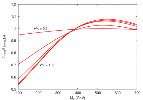
Figure 9: Ratio of the decay of a Higgs to $\gamma\gamma$ compared with the value in the SM. The different curves correspond to the values of $v/k$ from bottom to top on the left edge of the graph of (1.5, 1.1, 0.8, 0.4, 0.1). Again, we have taken $y_{\rm light}=1/10$.

This decay mode is shown in Fig. 9. Note that there is some suppression for low Higgs masses.

Putting all of this together we can compute the branching ratios, shown in Fig 10 for $v/k=1/10$, $y_{\rm light}=1/10$. Several features are visible. First, the $WW$ and $ZZ$ coupling suppression results in a delayed dominance of these modes, although they do dominate eventually for all allowed values of $v/k$. Second, the $Z_{2}$ left-right symmetry requires the $b$ and $t$ couplings to be equal, and hence the width to $b\bar{b}$ is always larger than the width to $t\bar{t}$ (they would, of course, be equal if $m_{t}=m_{b}$). Finally, this enhancement in the $b$ coupling suppresses all other modes. In particular, the $h\to\gamma\gamma$ mode is unobservable. Note that even if the $b$ coupling were not enhanced, the $\gamma\gamma$ mode would be reduced over a large region of parameter space by the $hWW$ coupling suppression. This means searches for Higgs bosons at the LHC which depend on the $h\to\gamma\gamma$ decay mode will have a reduced signal, and will possibly not be viable if this model is correct.

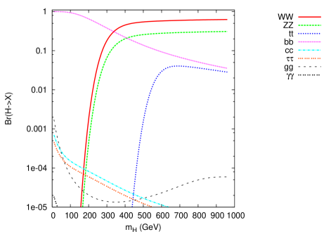
Figure 10: Partial widths (top) and branching ratios (bottom) for Higgs decay into various channels as a function of the Higgs mass at fixed $v/k=1/10$ and $y_{\rm light=1/10}$.

It has been observed that Higgsless models with KK masses $\gtrsim 1{\ \rm TeV}$ show a breakdown of perturbative unitarity in longitudinal gauge boson scattering [28]. Of course, in a purely Higgsed 4D model, unitarity is maintained to arbitrarily high scales. It is therefore interesting to see the behavior of the amplitude for $W_{L}W_{L}\to W_{L}W_{L}$ [57] as a function of $v/k$. This is shown in Fig. 11 for a fixed Higgs mass of $150{\ \rm GeV}$. Note both the rapid falloff and the fact that, in the region $v/k\leq 1/4$, unitarity is maintained to scales above 6 TeV.

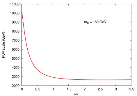
Figure 11: The center-of-mass energy at which tree-level perturbative unitarity is violated in $W^{+}_{L}W^{-}_{L}\to W^{+}_{L}W^{-}_{L}$ scattering.

6 Conclusion

In this paper we have investigated the effects of a finite Higgs vev in the Left-Right symmetric Randall-Sundrum model with fermions and gauge bosons in the bulk. The main effects come from distortions of the $W$ and $Z$ wavefunctions near the IR brane. We found that the model is free of existing constraints as long as $v/k\lesssim 1/4$. In this region the Higgs coupling to the gauge bosons can be suppressed by a factor of up to $1/3$, and the Higgs couplings to $gg$ and $\gamma\gamma$ can be substantially shifted. This results in a new pattern of branching ratios as a function of $m_{H}$.

It has been shown previously that the precision electroweak observables can be shifted by inclusion of brane localized kinetic terms for the gauge bosons and fermions [14, 12, 18]. This will shift the allowed region of $v/k$, but will not qualitatively alter the properties of the Higgs couplings. Additionally, it would be interesting to consider the effects of non-zero Higgs-radion mixing, which has been set to zero here.

In this model it may be difficult to discover the Higgs, since the $\gamma\gamma$ mode is invisible over much of the parameter space and the massive gauge boson couplings to the Higgs are reduced. However, when it is found the properties of the Higgs will be an important tool in mapping out the parameters of the full model.

Appendix A Bidoublet Higgs

Instead of the real bidoublet used in Section 2, we could use a complex bidoublet Higgs field, producing a version of the Two Higgs Doublet Model. We can parameterize this field as

$$\varphi=\begin{pmatrix}\varphi_{1}^{0}&\varphi_{1}^{+}\\ \varphi_{2}^{-}&\varphi_{2}^{0}\\ \end{pmatrix}$$ (41)

The most general form of the potential for complex bidoublet field is [58]

$$V(\varphi) =-\mu^{2}{\rm Tr}\varphi^{\dagger}\varphi+\lambda_{1}({\rm Tr}\varphi^{\dagger}\varphi)^{2}+\lambda_{2}{\rm Tr}\varphi^{\dagger}\varphi\varphi^{\dagger}\varphi+\frac{1}{2}\lambda_{3}({\rm Tr}\varphi^{\dagger}\tilde{\varphi}+{\rm Tr}\tilde{\varphi}^{\dagger}\varphi)^{2}$$

$$+\frac{1}{2}\lambda_{4}({\rm Tr}\varphi^{\dagger}-{\rm Tr}\tilde{\varphi}^{\dagger}\varphi)^{2}+\lambda_{5}{\rm Tr}\varphi^{\dagger}\varphi\tilde{\varphi}^{\dagger}\tilde{\varphi}+\frac{1}{2}\lambda_{6}({\rm Tr}\varphi^{\dagger}\tilde{\varphi}\varphi^{\dagger}\tilde{\varphi}+{\rm Tr}\tilde{\varphi}^{\dagger}\varphi\tilde{\varphi}^{\dagger}\varphi),$$ (42)

where $\tilde{\varphi}=\sigma_{2}\varphi^{*}\sigma_{2}$, and $\sigma_{2}$ is the ordinary Pauli matrix. We expect that there will be solutions where the neutral fields acquire vevs, so we try $\langle\varphi^{0}_{1}\rangle=v_{1}$, $\langle\varphi^{0}_{2}\rangle=v_{2}$. Stability of this solution requires the two conditions $\partial V/\partial v_{1,2}=0$, where all fields are evaluated at their vevs. These then imply

$$\left({v_{1}}^{2}-{v_{2}}^{2}\right)\left(-4\,{\lambda_{3}}-{\lambda_{5}}+{\lambda_{2}}-{\lambda_{6}}\right)=0.$$ (43)

There is no symmetry that can require the second factor to vanish, so we can see that aside from a vanishingly small and unnatural region of parameter space we have $v^{2}_{1}=v^{2}_{2}\equiv v^{2}/2$. The second stability condition then gives

$$v^{2}=\frac{1}{2}\,{\frac{{\mu}^{2}}{4\,{\lambda_{3}}+2\,{\lambda_{1}}+{\lambda_{2}}+{\lambda_{5}}+{\lambda_{6}}}}.$$ (44)

Inserting this solution into Eq. (42) we can read off that the mass eigenstates are

$$h \equiv\Re(\varphi^{0}_{1}+\varphi^{0}_{2}) H \equiv\Re(\varphi^{0}_{1}-\varphi^{0}_{2})$$

$$A \equiv\Im(\varphi^{0}_{1}+\varphi^{0}_{2}) G^{0} \equiv\Im(\varphi^{0}_{1}-\varphi^{0}_{2})$$

$$h^{+} \equiv\varphi^{+}_{1}+\varphi^{+}_{2} G^{+} \equiv\varphi^{+}_{1}-\varphi^{+}_{2}.$$ (45)

The $G^{i}$ are the would-be Goldstone fields, and hence have no mass terms in the potential. Furthermore, the structure of the potential requires $m_{H}=m_{h^{+}}$. However, there are enough parameters that the masses are otherwise arbitrary. To parameterize this, we can write

$$m_{h}^{2}=\lambda_{h}v^{2},\qquad m_{H}^{2}=m_{h^{+}}^{2}=\lambda_{H}v^{2},\qquad m_{A}^{2}=\lambda_{A}v^{2}.$$ (46)

CP symmetry tells us that there is no three-point vertex coupling two gauge bosons to the CP-odd scalar. Hence, restricting ourselves to the neutral sector, we find the analysis from the main part of the paper goes through with minimal changes.

References

- [1] N. Arkani-Hamed, S. Dimopoulos, and G. R. Dvali, The hierarchy problem and new dimensions at a millimeter, Phys. Lett. B429 (1998) 263–272, [hep-ph/9803315].
- [2] I. Antoniadis, A possible new dimension at a few TeV, Phys. Lett. B246 (1990) 377–384.
- [3] L. Randall and R. Sundrum, A large mass hierarchy from a small extra dimension, Phys. Rev. Lett. 83 (1999) 3370–3373, [hep-ph/9905221].
- [4] H. Davoudiasl, J. L. Hewett, and T. G. Rizzo, Phenomenology of the Randall-Sundrum gauge hierarchy model, Phys. Rev. Lett. 84 (2000) 2080, [hep-ph/9909255].
- [5] H. Davoudiasl, J. L. Hewett, and T. G. Rizzo, Bulk gauge fields in the Randall-Sundrum model, Phys. Lett. B473 (2000) 43–49, [hep-ph/9911262].
- [6] Y. Grossman and M. Neubert, Neutrino masses and mixings in non-factorizable geometry, Phys. Lett. B474 (2000) 361–371, [hep-ph/9912408].
- [7] H. Davoudiasl, J. L. Hewett, and T. G. Rizzo, Experimental probes of localized gravity: On and off the wall, Phys. Rev. D63 (2001) 075004, [hep-ph/0006041].
- [8] A. Pomarol, Gauge bosons in a five-dimensional theory with localized gravity, Phys. Lett. B486 (2000) 153–157, [hep-ph/9911294].
- [9] T. Gherghetta and A. Pomarol, Bulk fields and supersymmetry in a slice of ads, Nucl. Phys. B586 (2000) 141–162, [hep-ph/0003129].
- [10] J. L. Hewett, F. J. Petriello, and T. G. Rizzo, Precision measurements and fermion geography in the randall-sundrum model revisited, JHEP 09 (2002) 030, [hep-ph/0203091].
- [11] C. Csaki, J. Erlich, and J. Terning, The effective lagrangian in the Randall-Sundrum model and electroweak physics, Phys. Rev. D66 (2002) 064021, [hep-ph/0203034].
- [12] M. Carena, T. M. P. Tait, and C. E. M. Wagner, Branes and orbifolds are opaque, Acta Phys. Polon. B33 (2002) 2355, [hep-ph/0207056].
- [13] M. Carena, E. Ponton, T. M. P. Tait, and C. E. M. Wagner, Opaque branes in warped backgrounds, Phys. Rev. D67 (2003) 096006, [hep-ph/0212307].
- [14] H. Davoudiasl, J. L. Hewett, and T. G. Rizzo, Brane localized kinetic terms in the Randall-Sundrum model, Phys. Rev. D68 (2003) 045002, [hep-ph/0212279].
- [15] S. J. Huber, Flavor violation and warped geometry, Nucl. Phys. B666 (2003) 269–288, [hep-ph/0303183].
- [16] M. E. Peskin and T. Takeuchi, A new constraint on a strongly interacting Higgs sector, Phys. Rev. Lett. 65 (1990) 964–967.
- [17] K. Agashe, A. Delgado, M. J. May, and R. Sundrum, RS1, custodial isospin and precision tests, JHEP 08 (2003) 050, [hep-ph/0308036].
- [18] M. Carena, A. Delgado, E. Ponton, T. M. P. Tait, and C. E. M. Wagner, Warped fermions and precision tests, Phys. Rev. D71 (2005) 015010, [hep-ph/0410344].
- [19] K. Agashe and G. Servant, Warped unification, proton stability and dark matter, Phys. Rev. Lett. 93 (2004) 231805, [hep-ph/0403143].
- [20] K. Agashe and G. Servant, Baryon number in warped GUTs: Model building and (dark matter related) phenomenology, hep-ph/0411254.
- [21] C. Csaki, C. Grojean, H. Murayama, L. Pilo, and J. Terning, Gauge theories on an interval: Unitarity without a Higgs, Phys. Rev. D69 (2004) 055006, [hep-ph/0305237].
- [22] C. Csaki, C. Grojean, L. Pilo, and J. Terning, Towards a realistic model of Higgsless electroweak symmetry breaking, Phys. Rev. Lett. 92 (2004) 101802, [hep-ph/0308038].
- [23] Y. Nomura, Higgsless theory of electroweak symmetry breaking from warped space, JHEP 11 (2003) 050, [hep-ph/0309189].
- [24] C. Csaki, C. Grojean, J. Hubisz, Y. Shirman, and J. Terning, Fermions on an interval: Quark and lepton masses without a Higgs, Phys. Rev. D70 (2004) 015012, [hep-ph/0310355].
- [25] R. Barbieri, A. Pomarol, and R. Rattazzi, Weakly coupled Higgsless theories and precision electroweak tests, Phys. Lett. B591 (2004) 141–149, [hep-ph/0310285].
- [26] H. Davoudiasl, J. L. Hewett, and T. G. Rizzo, Brane localized curvature for warped gravitons, JHEP 08 (2003) 034, [hep-ph/0305086].
- [27] T. Ohl and C. Schwinn, Unitarity, BRST symmetry and Ward identities in orbifold gauge theories, Phys. Rev. D70 (2004) 045019, [hep-ph/0312263].
- [28] H. Davoudiasl, J. L. Hewett, B. Lillie, and T. G. Rizzo, Higgsless electroweak symmetry breaking in warped backgrounds: Constraints and signatures, Phys. Rev. D70 (2004) 015006, [hep-ph/0312193].
- [29] H. Davoudiasl, J. L. Hewett, B. Lillie, and T. G. Rizzo, Warped Higgsless models with IR-brane kinetic terms, JHEP 05 (2004) 015, [hep-ph/0403300].
- [30] J. L. Hewett, B. Lillie, and T. G. Rizzo, Monte carlo exploration of warped Higgsless models, JHEP 10 (2004) 014, [hep-ph/0407059].
- [31] C. Schwinn, Higgsless fermion masses and unitarity, Phys. Rev. D69 (2004) 116005, [hep-ph/0402118].
- [32] G. Cacciapaglia, C. Csaki, C. Grojean, and J. Terning, Oblique corrections from Higgsless models in warped space, Phys. Rev. D70 (2004) 075014, [hep-ph/0401160].
- [33] J. Hirn and J. Stern, The role of spurions in Higgs-less electroweak effective theories, Eur. Phys. J. C34 (2004) 447–475, [hep-ph/0401032].
- [34] A. Birkedal, K. Matchev, and M. Perelstein, Collider phenomenology of the Higgsless models, hep-ph/0412278.
- [35] R. S. Chivukula, E. H. Simmons, H.-J. He, M. Kurachi, and M. Tanabashi, Universal non-oblique corrections in Higgsless models and beyond, Phys. Lett. B603 (2004) 210–218, [hep-ph/0408262].
- [36] R. S. Chivukula, E. H. Simmons, H.-J. He, M. Kurachi, and M. Tanabashi, The structure of corrections to electroweak interactions in Higgsless models, Phys. Rev. D70 (2004) 075008, [hep-ph/0406077].
- [37] R. S. Chivukula, E. H. Simmons, H.-J. He, M. Kurachi, and M. Tanabashi, Deconstructed Higgsless models with one-site delocalization, hep-ph/0502162.
- [38] R. S. Chivukula, H.-J. He, M. Kurachi, E. H. Simmons, and M. Tanabashi, Ideal fermion delocalization in Higgsless models, hep-ph/0504114.
- [39] R. Sekhar Chivukula, E. H. Simmons, H.-J. He, M. Kurachi, and M. Tanabashi, Electroweak corrections and unitarity in linear moose models, hep-ph/0410154.
- [40] R. Casalbuoni, S. De Curtis, and D. Dominici, Moose models with vanishing S parameter, Phys. Rev. D70 (2004) 055010, [hep-ph/0405188].
- [41] N. Evans and P. Membry, Higgless W unitarity from decoupling deconstruction, hep-ph/0406285.
- [42] S. Gabriel, S. Nandi, and G. Seidl, 6D Higgsless standard model, hep-ph/0406020.
- [43] G. Cacciapaglia, C. Csaki, C. Grojean, M. Reece, and J. Terning, Top and bottom: A brane of their own, hep-ph/0505001.
- [44] J. M. Maldacena, The large N limit of superconformal field theories and supergravity, Adv. Theor. Math. Phys. 2 (1998) 231–252, [hep-th/9711200].
- [45] G. Burdman and Y. Nomura, Holographic theories of electroweak symmetry breaking without a Higgs boson, Phys. Rev. D69 (2004) 115013, [hep-ph/0312247].
- [46] K. Agashe, R. Contino, and A. Pomarol, The minimal composite Higgs model, hep-ph/0412089.
- [47] K. Agashe, R. Contino, and R. Sundrum, Top compositeness and precision unification, hep-ph/0502222.
- [48] G. F. Giudice, R. Rattazzi, and J. D. Wells, Graviscalars from higher-dimensional metrics and curvature- higgs mixing, Nucl. Phys. B595 (2001) 250–276, [hep-ph/0002178].
- [49] C. Csaki, M. L. Graesser, and G. D. Kribs, Radion dynamics and electroweak physics, Phys. Rev. D63 (2001) 065002, [hep-th/0008151].
- [50] LEP Collaboration, A combination of preliminary electroweak measurements and constraints on the standard model, hep-ex/0312023.
- [51] D0 Collaboration, V. M. Abazov et. al., Search for heavy particles decaying into electron positron pairs in p anti-p collisions, Phys. Rev. Lett. 87 (2001) 061802, [hep-ex/0102048].
- [52] ALEPH Collaboration, R. Barate et. al., Search for the standard model higgs boson at lep, Phys. Lett. B565 (2003) 61–75, [hep-ex/0306033].
- [53] T. G. Rizzo, Decays of heavy Higgs bosons, Phys. Rev. D22 (1980) 722.
- [54] F. J. Petriello, Kaluza-klein effects on Higgs physics in universal extra dimensions, JHEP 05 (2002) 003, [hep-ph/0204067].
- [55] J. F. Gunion, H. E. Haber, G. L. Kane, and S. Dawson, The Higgs hunter’s guide, . SCIPP-89/13.
- [56] G. Passarino and M. J. G. Veltman, One loop corrections for e+ e- annihilation into mu+ mu- in the weinberg model, Nucl. Phys. B160 (1979) 151.
- [57] M. J. Duncan, G. L. Kane, and W. W. Repko, W W physics at future colliders, Nucl. Phys. B272 (1986) 517.
- [58] J. F. Gunion, J. Grifols, A. Mendez, B. Kayser, and F. I. Olness, Higgs bosons in left-right symmetric models, Phys. Rev. D40 (1989) 1546.