Predictions of $pp,\bar{p}p$ total cross section and
$\rho$ ratio at LHC and cosmic-ray energies

Abstract

We propose to use rich informations on the $pp,\bar{p}p$ total cross sections $\sigma_{\rm tot}$ below $N(\sim 10)$GeV in order to predict the total cross section and $\rho$ ratio at very high energies. Using the FESR as a constraint for high energy parameters, we search for the simultaneous best fit to the data points of $\sigma_{\rm tot}$ and $\rho$ ratio up to some energy (e.g., ISR, Tevatron) to determine the high-energy parameters. We then predict $\sigma_{\rm tot}$ and $\rho$ in the LHC and high-energy cosmic-ray regions. Using the data up to $\sqrt{s}=1.8$TeV(Tevatron), we predict $\sigma_{\rm tot}^{pp}$ and $\rho^{pp}$ at the LHC energy($\sqrt{s}=14$TeV) as $106.3\pm 5.1_{\rm syst}\pm 2.4_{\rm stat}$mb and $0.126\pm 0.007_{\rm syst}\pm 0.004_{\rm stat}$, respectively. The predicted values of $\sigma_{\rm tot}$ in terms of the same parameters are in good agreement with the cosmic-ray experimental data sample up to $P_{lab}\sim 10^{8\sim 9}$GeV by Block, Halzen, and Stanov.

Recently[1], we have proposed to use rich informations on $\pi p$ total cross sections below N($\sim$10 GeV) in addition to high-energy data to discriminate whether these cross sections increase like log $\nu$ or log${}^{2}\ \nu$ at high energies[2]. The FESR which was derived in the spirit of the $P^{\prime}$ sum rule[3] as well as the $n=1$ moment FESR([4], [5]) have been required to constrain the high-energy parameters. We then searched for the best fit of $\sigma_{\rm tot}^{(+)}$ above 70GeV in terms of high-energy parameters constrained by the two FESR. We then arrived at the conclusion that our analysis prefers the log${}^{2}\nu$ behaviours consistent with the Froissart-Martin unitarity bound[6].

As for the $\bar{p}p$ and $pp$ total cross sections, there are a lot of data including cosmic-ray data up to $\sqrt{s}\sim$ several times of $10^{4}$GeV compared with data up to $\sqrt{s}\sim$30GeV for $\pi N$ scattering. Therefore, it is very valuable if one could investigate the high-energy behaviours at LHC and cosmic-ray regions[8] using the similar approach as ref. [1].

(The purpose of this Letter):   The purpose of this Letter is to predict $\sigma_{\rm tot}^{(+)}$, the $\bar{p}p$, $pp$ total cross sections and $\rho^{(+)}$, the ratio of the real to imaginary part of the forward scattering amplitude at the LHC and the higher-energy cosmic-ray regions, using the experimental data for $\sigma_{\rm tot}^{(+)}$ and $\rho^{(+)}$ for 70GeV$<P_{lab}<P_{large}$ as inputs. We first choose $P_{large}=2100$GeV corresponding to ISR region($\sqrt{s}\simeq 60$GeV). Secondly we choose $P_{large}=2\times 10^{6}$GeV corresponding to the Tevatron collider ($\sqrt{s}\simeq 2$TeV). In a recent paper, Block and Halzen[7] emphasized the importance of $\rho$ for the evidence for saturation of the Froissart-Martin bound[6]. We also use the $\rho$ ratio as input data in addition to FESR as a constraint. We searched for the simultaneous best fit of $\sigma_{\rm tot}^{(+)}$ and $\rho^{(+)}$ in terms of high-energy parameters $c_{0},c_{1},c_{2}$ and $\beta_{P^{\prime}}$ constrained by the FESR. It turns out that the prediction of $\sigma_{\rm tot}^{(+)}$ agrees with $pp$ experimental data at these cosmic-ray energy regions[8, 22] within errors in the first case ( ISR ). It has to be noted that the energy range of predicted $\sigma_{\rm tot}^{(+)}$, $\rho^{(+)}$ is several orders of magnitude larger than the energy region of $\sigma_{\rm tot}^{(+)}$, $\rho^{(+)}$ input (see Fig. 1). If we use data up to Tevatron (the second case), the situation is much improved, although there are some systematic uncertainties coming from the data at $\sqrt{s}=1.8$TeV (see Fig. 2).

FESR(1): Firstly we derive the FESR in the spirit of the $P^{\prime}$ sum rule [3]. Let us consider the crossing-even forward scattering amplitude defined by

$$F^{(+)}(\nu) = \frac{f^{\bar{p}p}(\nu)+f^{pp}(\nu)}{2}\ \ {\rm with}\ \ Im\ F^{(+)}(\nu)=\frac{k\ \sigma^{(+)}_{\rm tot}(\nu)}{4\pi}\ .$$ (1)

We also assume

$$Im\ F^{(+)}(\nu) = Im\ R(\nu)+Im\ F_{P^{\prime}}(\nu)$$ (2)

$$= \frac{\nu}{M^{2}}\left(c_{0}+c_{1}{\rm log}\frac{\nu}{M}+c_{2}{\rm log}^{2}\frac{\nu}{M}\right)+\frac{\beta_{P^{\prime}}}{M}\left(\frac{\nu}{M}\right)^{\alpha_{P^{\prime}}}\ \ \ \ \$$

at high energies ($\nu>N$). We have defined the functions $R(\nu)$ and $F_{P^{\prime}}(\nu)$ by replacing $\mu$ by M in Eq. (3) of ref.[1]. Here, $M$ is the proton( anti-proton) mass and $\nu,\ k$ are the incident proton(anti-proton) energy, momentum in the laboratory system, respectively.

Since the amplitude is crossing-even, we have

$$R(\nu) = \frac{i\nu}{2M^{2}}\left\{2c_{0}+c_{2}\pi^{2}+c_{1}\left({\rm log}\frac{e^{-i\pi}\nu}{M}+{\rm log}\frac{\nu}{M}\right)\right.$$ (3)

$$\left.+c_{2}\left({\rm log}^{2}\frac{e^{-i\pi}\nu}{M}+{\rm log}^{2}\frac{\nu}{M}\right)\right\}\ ,\ \ \ \ \ \ \$$

$$F_{P^{\prime}}(\nu) = -\frac{\beta_{P^{\prime}}}{M}\left(\frac{(e^{-i\pi}\nu/M)^{\alpha_{P^{\prime}}}+(\nu/M)^{\alpha_{P^{\prime}}}}{{\rm sin}\pi\alpha_{P^{\prime}}}\right),$$ (4)

and subsequently obtain

$$Re\ R(\nu) = \frac{\pi\nu}{2M^{2}}\left(c_{1}+2c_{2}{\rm log}\frac{\nu}{M}\right)\ ,\ \ \$$ (5)

$$Re\ F_{P^{\prime}}(\nu) = -\frac{\beta_{P^{\prime}}}{M}\left(\frac{\nu}{M}\right)^{0.5}\ ,\ \ \$$ (6)

substituting $\alpha_{P^{\prime}}=\frac{1}{2}$ in Eq. (4). Let us define

$$\tilde{F}^{(+)}(\nu) = F^{(+)}(\nu)-R(\nu)-F_{P^{\prime}}(\nu)\sim\nu^{\alpha(0)}\ (\alpha(0)<0)\ .$$ (7)

Using the similar technique to ref.[1], we obtain

$$Re\ \tilde{F}^{(+)}(M) = \frac{2P}{\pi}\int_{0}^{\infty}\frac{\nu Im\ \tilde{F}^{(+)}(\nu)}{k^{2}}d\nu\$$ (8)

$$= \frac{2P}{\pi}\int_{0}^{M}\frac{\nu}{k^{2}}Im\ F^{(+)}(\nu)d\nu+\frac{1}{2\pi^{2}}\int_{0}^{\overline{N}}\sigma_{\rm tot}^{(+)}(k)dk\$$

$$-\frac{2P}{\pi}\int_{0}^{N}\frac{\nu}{k^{2}}\left\{Im\ R(\nu)+\frac{\beta_{P^{\prime}}}{M}\left(\frac{\nu}{M}\right)^{0.5}\right\}d\nu\ ,$$

where $\overline{N}=\sqrt{N^{2}-M^{2}}\simeq N$. Let us call Eq. (8) as the FESR(1).

(FESR(2)): The second FESR corresponding to $n=1$ [5] is:

$$\int_{0}^{M}\nu Im\ F^{(+)}(\nu)d\nu+\frac{1}{4\pi}\int_{0}^{\overline{N}}k^{2}\sigma_{\rm tot}^{(+)}(k)dk$$

$$=\int_{0}^{N}\nu Im\ R(\nu)d\nu+\int_{0}^{N}\nu Im\ F_{P^{\prime}}(\nu)d\nu\ \ \ .\ \ \$$ (9)

We call Eq. (9) as the FESR(2) which we use in our analysis.

(The $\rho^{(+)}$ ratio): The $\rho^{(+)}$ ratio, the ratio of the real to imaginary part of $F^{(+)}(\nu)$ is obtained from Eqs. (2), (5) and (6) as

$$\rho^{(+)}(\nu) = \frac{Re\ F^{(+)}(\nu)}{Im\ F^{(+)}(\nu)}=\frac{Re\ R(\nu)+Re\ F_{P^{\prime}}(\nu)}{Im\ R(\nu)+Im\ F_{P^{\prime}}(\nu)}$$ (10)

$$= \frac{\frac{\pi\nu}{2M^{2}}\left(c_{1}+2c_{2}{\rm log}\frac{\nu}{M}\right)-\frac{\beta_{P^{\prime}}}{M}\left(\frac{\nu}{M}\right)^{0.5}}{\frac{k\sigma_{\rm tot}^{(+)}(\nu)}{4\pi}}\ .\ \ \$$

(General approach):   The FESR(1)(Eq. (8)) has some problem. i.e., there are the so-called unphysical regions coming from boson poles below the $\bar{p}p$ threshold. So, the contributions from unphysical regions of the first term of the right-hand side of Eq. (8) have to be calculated. Reliable estimates, however, are difficult. Therefore, we will not adopt the FESR(1).

On the other hand, contributions from the unphysical regions to the first term of the left-hand side of FESR(2)(Eq. (9)) can be estimated to be an order of 0.1% compared with the second term. Thus, it can easily be neglected.

Therefore, the FESR(2)(Eq. (9)), the formula of $\sigma_{\rm tot}^{(+)}$(Eqs. (1) and (2)) and the $\rho^{(+)}$ ratio (Eq. (10)) are our starting points. Armed with the FESR(2), we express high-energy parameters $c_{0},c_{1},c_{2},\beta_{P^{\prime}}$ in terms of the integral of total cross sections up to $N$. Using this FESR(2) as a constraint for $\beta_{P^{\prime}}=\beta_{P^{\prime}}(c_{0},c_{1},c_{2})$, the number of independent parameters is three. We then search for the simultaneous best fit to the data points of $\sigma_{\rm tot}^{(+)}(k)$ and $\rho^{(+)}(k)$ for 70GeV$\leq k\leq P_{large}$ to determine the values of $c_{0},c_{1},c_{2}$ giving the least $\chi^{2}$. We thus predict the $\sigma_{\rm tot}$ and $\rho^{(+)}$ in LHC energy and high-energy cosmic-ray regions.

(Data):   We use rich data[9] of $\sigma^{\bar{p}p}$ and $\sigma^{pp}$ to evaluate the relevant integrals of cross sections appearing in FESR(2). We connect the each data point of $k^{2}\sigma_{\rm tot}^{\bar{p}p}$ and $k^{2}\sigma_{\rm tot}^{pp}$ with the next point by a straight line in order, from $k=0$ to $k=\overline{N}$, and regard the area of this polygonal line graph as the relevant integral in the region $0\leq k\leq\overline{N}$. The integral of $k^{2}\sigma_{\rm tot}^{(+)}(k)$ is given by averaging those of $k^{2}\sigma_{\rm tot}^{\bar{p}p}(k)$ and $k^{2}\sigma_{\rm tot}^{pp}(k)$. We have obtained

$$\frac{1}{4\pi}\int_{0}^{\overline{N}}k^{2}\sigma_{\rm tot}^{(+)}(k)dk = 3403\pm 20\ {\rm GeV}.$$ (11)

for $\overline{N}=10$GeV (which corresponds to $\sqrt{s}=E_{cm}=4.54$GeV). The error of the integral, which is from the error of each data point, is very small (less than 1%), and thus, we regard the central value as an exact one in the following analysis.

When $\sigma^{\bar{p}p}_{\rm tot}$ and $\sigma^{pp}_{\rm tot}$ data points are listed at the same value of $k$, we make the $\sigma_{\rm tot}^{(+)}(k)$ data point by averaging these values. Totally, 37 points are obtained in the energy region, $0.54{\rm GeV}\leq k\leq 2100$GeV. The data point of maximum value $k=2094.03$GeV($\sqrt{s}=62.7$GeV) comes from ISR[10]. There are 12 points in the $70$GeV$\leq k\leq 2100$GeV (11.5GeV $\leq\sqrt{s}\leq$ 62.7GeV). There are no data reported in the wide range of $2100{\rm GeV}\leq k\leq 1\times 10^{5}$GeV. There are 6 points[11, 12, 15, 14, 13] of $\sigma^{\bar{p}p}_{\rm tot}$ in the Tevatron-collider energy region, $1\times 10^{5}{\rm GeV}\leq k\leq 2\times 10^{6}$GeV.

It is necessary to pay special attention to treat the data with the maximum $k=1.7266\times 10^{6}$GeV($\sqrt{s}=1.8$TeV) in this energy range, which comes from the three experiments E710[13]$/$E811[14] and CDF[15]. The former two experiments are mutually consistent and their averaged $\bar{p}p$ cross section is $\sigma_{\rm tot}^{\bar{p}p}=72.0\pm 1.7$mb, which deviates from the result of CDF experiment $\sigma_{\rm tot}^{\bar{p}p}=80.03\pm 2.24$mb.

Again there are no data reported in the range $2\times 10^{6}{\rm GeV}\leq k\leq 2\times 10^{7}$GeV. There are 7 points of $\sigma^{pp}_{\rm tot}$ with somewhat large errors, reported in the cosmic-ray energy region, $2\times 10^{7}{\rm GeV}\leq k\leq 5\times 10^{8}$GeV (6TeV $\leq\sqrt{s}\leq$ 30TeV), coming from cosmic-ray experiments[8, 22]. Totally we obtain 25 points of $\sigma^{(+)}_{\rm tot}$ in $k\geq$ 70GeV. We have not included the cosmic-ray data in our analysis. Thus, 18 points of $\sigma^{(+)}_{\rm tot}$ are used in the analyses.

The data of $\rho^{\bar{p}p}(k)(=Re\ f^{\bar{p}p}(k)/Im\ f^{\bar{p}p}(k))$ and $\rho^{pp}(k)(=Re\ f^{pp}(k)/Im\ f^{pp}(k))$ are reported in ref.[9]. When both data points are listed at the same value of $k$, we can make the $\rho^{(+)}(k)(=Re\ F^{(+)}(k)/Im\ F^{(+)}(k))$ data point. We obtain 9 points of $\rho^{(+)}$ in the energy region, $70{\rm GeV}\leq k\leq 2100$GeV. No data are reported in the range $2100{\rm GeV}\leq k\leq 1\times 10^{5}$GeV. The two points of $\rho^{\bar{p}p}$ are reported in Tevatron-collider energy region, $1\times 10^{5}{\rm GeV}\leq k\leq 2\times 10^{6}$GeV ( at $k=1.5597\times 10^{5}$GeV($\sqrt{s}=541$GeV)[17] and $k=1.7266\times 10^{6}$GeV($\sqrt{s}=$1.8TeV)[13] ). We regard these two points as the $\rho^{(+)}$ data. As a result, we obtain 11 points of $\rho^{(+)}$ up to Tevatron-collider energy region, $70{\rm GeV}\leq k\leq 2\times 10^{6}$GeV.

In the actual analyses, we use $Re\ F^{(+)}$ instead of $\rho^{(+)}(=Re\ F^{(+)}/Im\ F^{(+)})$. The data points of $Re\ F^{(+)}(k)$ are made by multiplying $\rho^{(+)}(k)$ by $Im\ F^{(+)}(k)=\frac{k}{8\pi}(\sigma_{\rm tot}^{\bar{p}p}(k)+\sigma_{\rm tot}^{pp}(k))$. The values of $\sigma^{\bar{p}p}_{\rm tot}$ and $\sigma^{pp}_{\rm tot}$ at the relevant values of $k$ are obtained as follows: For $k<1500$GeV, they are determined by the formula given in ref.[9](see the footnote 4). Two experimental values[12, 13] of $\sigma^{\bar{p}p}$ in the Tevatron region are used.

(Analysis):   As was explained in the general approach, both $\sigma_{\rm tot}^{(+)}$ and $Re\ F^{(+)}$ data in 70GeV $\leq k\leq P_{large}$ are fitted simultaneously through the formula Eq. (2) and Eq. (10) with the FESR(2)(Eq. (9)) as a constraint. FESR(2) with Eq. (11) gives us

$$8.87 = c_{0}+2.04c_{1}+4.26c_{2}+0.367\beta_{P^{\prime}}\ ,$$ (12)

which is used as a constraint of $\beta_{P^{\prime}}=\beta_{P^{\prime}}(c_{0},c_{1},c_{2})$, and the fitting is done by three parameters $c_{0},c_{1}$ and $c_{2}$.

We have done for the following three cases:
fit 1):    The fit to the data up to ISR energy region, 70GeV $\leq k\leq$ 2100GeV, which includes 12 points of $\sigma_{\rm tot}^{(+)}$ and 7 points of $\rho^{(+)}$.
fit 2):    The fit to the data up to Tevatron-collider energy region, 70GeV$\leq k\leq 2\times 10^{6}$GeV. For $k=1.7266\times 10^{6}$GeV($\sqrt{s}=1.8$TeV), the E710$/$E811 datum is used. There are 18 points of $\sigma_{\rm tot}^{(+)}$ and 9 points of $\rho^{(+)}$.
fit 3):    The same as fit 2, except for the CDF value at $\sqrt{s}=1.8$TeV used.

(Results of the fit):   The results are shown in Fig. 1(Fig. 2) for the fit 1(fit 2 and fit 3). The $\chi^{2}/d.o.f$ are given in Table 1. The reduced $\chi^{2}$ and the respective $\chi^{2}$-values devided by the number of data points for $\sigma_{\rm tot}^{(+)}$ and $\rho^{(+)}$ are less than or equal to unity. The fits are successful in all cases. There are some systematic differences between fit 2 and fit 3, which come from the experimental uncertainty of the data at $\sqrt{s}=1.8$TeV mentioned above.

Table 1: The values of $\chi^{2}$ for the fit 1 (fit up to ISR energy) and the fit 2 and fit 3 (fits up to Tevatron-collider energy). $N_{F}$ and $N_{\sigma}(N_{\rho})$ are the degree of freedom and the number of $\sigma^{(+)}_{\rm tot}(\rho^{(+)})$ data points in the fitted energy region.

	$\chi^{2}/N_{F}$	$\chi^{2}_{\sigma}/N_{\sigma}$	$\chi^{2}_{\rho}/N_{\rho}$
fit 1	10.6/15	3.6/12	7.0/7
fit 2	16.5/23	8.1/18	8.4/9
fit 3	15.9/23	9.0/18	6.9/9

Figure 1: Predictions for $\sigma^{(+)}$ and $\rho^{(+)}$ in terms of the fit 1. The fit is done for the data up to the ISR energy, in the region 70GeV$\leq$ $k$ $\leq$ 2100GeV (11.5GeV $\leq\sqrt{s}\leq$ 62.7GeV) which is shown by the arrow in each figure. Total cross section $\sigma^{(+)}_{\rm tot}$

in (a) all energy region, versus log${}_{10}P_{lab}/$GeV, (b) low energy region (up to ISR energy), versus $P_{lab}/$GeV and (c) high energy (Tevatron-collider, LHC and cosmic-ray energy) region, versus center of mass energy $E_{cm}$ in TeV unit. (d) gives the $\rho^{(+)}(=Re\ F^{(+)}/Im\ F^{(+)})$ in high energy region, versus $E_{cm}$ in terms of TeV. The thin dot-dashed lines represent the one standard deviation.

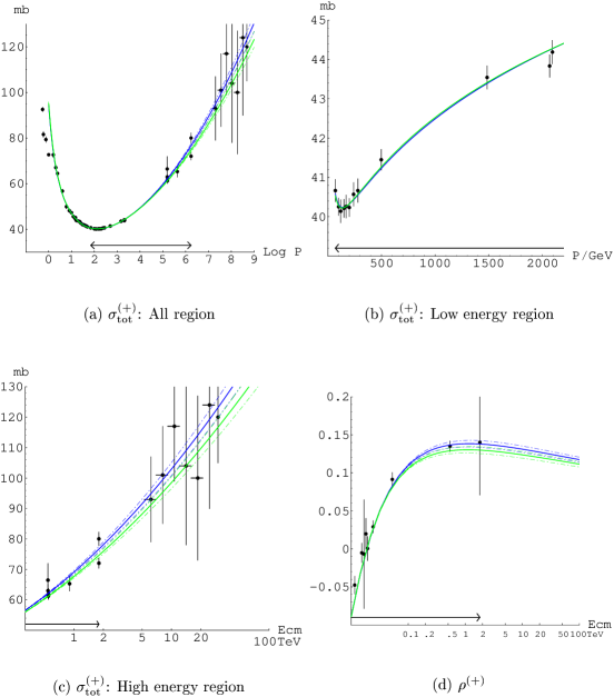
Figure 2: Predictions for $\sigma^{(+)}$ and $\rho^{(+)}$ in terms of the fit 2(shown by green lines) and fit 3(shown by blue lines). The fit is done for the data up to Tevatron-collider energy, in the region 70GeV$\leq$ $k$ $\leq$ $2\times 10^{6}$GeV(11.5GeV $\leq\sqrt{s}\leq$ 1.8TeV) which is shown by the arrow. For $k=1.7266\times 10^{6}$GeV($\sqrt{s}=E_{\rm cm}=1.8$TeV), the averaged datum of E710[13]/E811[14], $\sigma_{\rm tot}^{\bar{p}p}=72.0\pm 1.7$mb, is used in fit 2, while the $\sigma_{\rm tot}^{\bar{p}p}=80.03\pm 2.24$mb of CDF[15] is used in fit 3. For each figure, see the caption in Fig.1.

The best-fit values of the parameters are given in Table 2. Here the errors of one standard deviation are also given.

Table 2: The best-fit values of parameters in the fit 1, fit 2 and fit 3.

	$c_{2}$	$c_{1}$	$c_{0}$	$\beta_{P^{\prime}}$
fit 1	$0.0411\pm 0.0199$	$-0.074\mp 0.287$	$5.92\pm 1.07$	$7.96\mp 1.55$
fit 2	$0.0412\pm 0.0041$	$-0.076\mp 0.069$	$5.93\pm 0.28$	$7.95\mp 0.44$
fit 3	$0.0484\pm 0.0043$	$-0.181\mp 0.071$	$6.33\pm 0.29$	$7.37\mp 0.45$

(Predictions for $\sigma^{(+)}$ and $\rho^{(+)}$ at LHC and cosmic-ray energy region):   By using the values of parameters in Table 2, we can predict the $\sigma_{\rm tot}^{(+)}$ and $\rho^{(+)}$ in higher energy region, as are shown, respectively in (c) and (d) of Fig. 1 and 2. The thin dot-dashed lines represent the one standard deviation.

As is seen in (c) and (d) of Fig. 1, the fit 1 leads to the prediction of $\sigma_{\rm tot}^{(+)}$ and $\rho^{(+)}$ with somewhat large errors in the Tevatron-collider energy region, although the best-fit curves are consistent with the present experimental data in this region. Furthermore, the predicted values of $\sigma_{\rm tot}^{(+)}$ agree with $pp$ experimental data at the cosmic-ray energy regions[8, 22] within errors (see (a),(c) of Fig. 1). The best-fit curve gives $\chi^{2}/$(number of data) to be 13.0/16, and the prediction is successful. As was mentioned in the purpose of this Letter, it has to be noted that the energy range of predicted $\sigma_{\rm tot}^{(+)}$ is several orders of magnitude larger than the energy region of the $\sigma_{\rm tot}^{(+)}$, $\rho^{(+)}$ input. If we use data up to Tevatron-collider energy region as in the fit 2 and fit 3, the situation is much improved (see (a),(c) of Fig. 2), although there is systematic uncertainty depending on the treatment of the data at $\sqrt{s}=1.8$TeV.

The best-fit curve gives $\chi^{2}/$(number of data) from cosmic-ray data, 1.3/7(1.0/7) for fit 2(fit 3).

We can predict the values of $\sigma_{\rm tot}^{(+)}$ and $\rho^{(+)}$ at LHC energy, $\sqrt{s}$=$E_{cm}$=14TeV and at very high energy of cosmic-ray region. The relevant energies are very high, and the $\sigma_{\rm tot}^{(+)}$ and $\rho^{(+)}$ can be regarded to be equal to the $\sigma_{\rm tot}^{pp}$ and $\rho^{pp}$. The results are shown in Table 3.

Table 3: The predictions of $\sigma_{\rm tot}^{(+)}$ and $\rho^{(+)}$ at LHC energy $\sqrt{s}=E_{cm}=14$TeV($P_{lab}$=1.04$\times 10^{8}$GeV), and at a very high energy $P_{lab}=5\cdot 10^{20}$eV ($\sqrt{s}$=$E_{cm}$=967TeV.) in cosmic-ray region.

	$\sigma_{\rm tot}^{(+)}$($\sqrt{s}$=14TeV)	$\rho^{(+)}$($\sqrt{s}$=14TeV)	$\sigma_{\rm tot}^{(+)}$($P_{lab}$=$5\cdot 10^{20}$eV)	$\rho^{(+)}$($P_{lab}$=$5\cdot 10^{20}$eV)
fit 1	$103.8\pm 14.3$mb	$0.122\stackrel{{\scriptstyle+0.018}}{{\scriptstyle-0.024}}$	$188\pm 43$mb	$0.099\stackrel{{\scriptstyle+0.011}}{{\scriptstyle-0.017}}$
fit 2	$103.8\pm 2.3$mb	$0.122\pm 0.004$	$189\pm 8$mb	$0.100\pm 0.003$
fit 3	$108.9\pm 2.4$mb	$0.129\pm 0.004$	$204\pm 8$mb	$0.104\pm 0.003$

The prediction by the fit 1 in which data up to the ISR energy are used as input has somewhat large(fairly large) errors at LHC energy(at high energy of cosmic ray). By including the data up to the Tevatron collider, the prediction of fit 2(using E710/E811 datum) is smaller than that of fit 3(using CDF datum). We regard the difference between the results of fit 2 and fit 3 as the systematic uncertainties of our predictions. As a result, we predict

$$\sigma_{\rm tot}^{pp} = 106.3\pm 5.1_{\rm syst}\pm 2.4_{\rm stat}\ {\rm mb},\ \ \rho^{pp}=0.126\pm 0.007_{\rm syst}\pm 0.004_{\rm stat}\ \ \ \ \ \ \ \$$ (13)

at LHC energy($\sqrt{s}=E_{cm}=14$TeV). We obtain fairly large systematic errors coming from the experimental unceratinty at $\sqrt{s}=1.8$ TeV.

The predicted central value of $\sigma_{\rm tot}^{pp}$ is in good agreement with Block and Halzen[18] $\sigma_{\rm tot}^{pp}=107.4\pm 1.2$ mb, $\rho^{pp}=0.132\pm 0.001$. In contrary to our results( see Fig. 2(a), (c)), however, their values are not affected so much about CDF, E710/E811 discrepancy. Our prediction has also to be compared with Cudell et al.[23] $\sigma_{\rm tot}^{pp}=111.5\pm 1.2_{\rm syst}\stackrel{{\scriptstyle+4.1}}{{\scriptstyle-2.1}}_{\rm stat}$ mb, $\rho^{pp}=0.1361\pm 0.0015_{\rm syst}\stackrel{{\scriptstyle+0.0058}}{{\scriptstyle-0.0025}}_{\rm stat}$, who’s fitting techniques favours the CDF point at $\sqrt{s}=1.8$ TeV.

Finally we emphasize that precise measurements of both $\sigma_{\rm tot}^{pp}$ and $\rho^{pp}$ in the coming LHC experiments will resolve the FNAL discrepancy of $\sigma_{\rm tot}^{pp}$ ( Fig. 2(a), (c)). The LHC measurements would also clarify which is the best solution among the three high-energy cosmic-ray samples[20, 21, 22].
Note added in proof: After completion of the hep-ph/0505058, we were informed that M. M. Block and F. Halzen[18] have also done the similar work based on the same spirit of duality using different method independently. We were also informed by M. J. Menon[19] about other cosmic-ray analyses by Gaisser et al.[20] and N. N. Nikolaev[21] besides M. M. Block et al.[22] which are used as cosmic-ray data in this Letter.

References

- [1] K. Igi and M. Ishida, Phys. Rev. D 66 (2002) 034023.
- [2] J. R. Cudell et al., Phys. Rev. D 61 (2000) 034019.
- [3] K. Igi, Phys. Rev. Lett. 9 (1962) 76.
- [4] K. Igi and S. Matsuda, Phys. Rev. Lett. 18 (1967) 625.
- [5] R. Dolen, D. Horn and C. Schmid, Phys. Rev. 166 (1968) 1768. This paper includes references on earlier papers on FESR.
-
[6]
M. Froissart, Phys. Rev. 123 (1961) 1053.
A. Martin, Nuovo Cim. 42 (1966) 930. - [7] M. M. Block and F. Halzen, Phys. Rev. D 70 (2004) 091901.
-
[8]
M. Honda et al., Phys. Rev. Lett. 70 (1993) 525.
R. M. Baltrusaitis et al., Phys. Rev. Lett. 52 (1984) 1380. - [9] Particle Data Group, S. Eidelman et al., Phys. Lett. B 592 (2004) 313.
-
[10]
G. Carboni et al., Nucl. Phys. B 254 (1984) 697.
U. Amaldi et al., Nucl. Phys. B 145 (1978) 367. -
[11]
G. Arnison et al., UA1 Collaboration, Phys. Lett. B 128 (1983) 336.
R. Battiston et al., UA4 Collaboration, Phys. Lett. B 117 (1982) 126.
M. Bozzo et al., UA4 Collaboration, Phys. Lett. B 147 (1984) 392.
G. J. Alner et al., UA5 Collaboration, Zeit. Phys. C 32 (1986) 153. - [12] C. Augier et al., Phys. Lett. B 344 (1995) 451.
- [13] N. A. Amos et al., E-710 Collaboration, Phys. Rev. Lett. 68 (1992) 2433.
- [14] C. Avila et al., E-811 Collaboration, Phys. Lett. B 445 (1999) 419.
- [15] F. Abe et al., CDF Collaboration, Phys. Rev. D 50 (1994) 5550.
- [16] N. Amos et al., Nucl. Phys. B 262 (1985) 689.
- [17] C. Augier et al., Phys. Lett. B 316 (1993) 448.
- [18] M. M. Block and F. Halzen, hep-ph/0506031.
- [19] E. G. S. Luna and M. J. Menon, Phys. Lett. B 565(2003) 123.
- [20] T. K. Gaisser et al., Phys. Rev. D 36 (1987) 1350
- [21] N. N. Nikolaev, Phys. Rev. D 48 (1993) R1904.
- [22] M. M. Block et al., Phys. Rev. D 62 (2000) 077501.
- [23] J. R. Cudell et al., Phys. Rev. Lett. 89 (2002) 201801.