The Last of the Finite Loop Amplitudes in QCD

Abstract

We use on-shell recursion relations to determine the one-loop QCD scattering amplitudes with a massless external quark pair and an arbitrary number ($n-2$) of positive-helicity gluons. These amplitudes are the last of the unknown infrared- and ultraviolet-finite loop amplitudes of QCD. The recursion relations are similar to ones applied at tree level, but contain new non-trivial features corresponding to poles present for complex momentum arguments but absent for real momenta. We present the relations and the compact solutions to them, valid for all $n$. We also present compact forms for the previously-computed one-loop $n$-gluon amplitudes with a single negative helicity and the rest positive helicity.

I Introduction

The computation of new one-loop amplitudes in perturbative gauge theories, and in QCD in particular, will be a prerequisite for theoretical studies related to the experimental program at CERN’s upcoming Large Hadron Collider (LHC). The discovery and study of new physics beyond the standard $SU(3)\times SU(2)\times U(1)$ model of particle interactions will depend on our ability to calculate higher-order corrections to a wide variety of processes in its component gauge theories. Computations of tree-level scattering amplitudes are a first but insufficient step. The size and scale-variation of the strong coupling constant imply that a basic quantitative understanding must also include the one-loop amplitudes which enter into next-to-leading order corrections to cross sections. Such corrections are also required to build a theoretical base for a program of precision measurements at hadron colliders GloverReview . Precision measurements at the SLAC Linear Collider (SLC) and CERN’s Large Electron Positron (LEP) collider have proven the power of such a program in advancing our understanding of short-distance physics.

Recent years have seen important progress in this theoretical program; yet a wide and seemingly hostile province still severs us from our goal, encouraging us to seek additional tools for performing the required calculations. The last year in particular has seen new progress in the computation of tree-level CSW ; Higgs ; Currents ; RSVNewTree ; BCFRecurrence ; BCFW ; LuoWen ; BFRSV ; BadgerMassive and one-loop BST ; BCF7 ; NeqFourSevenPoint ; BCFII ; NeqFourNMHV ; OtherGaugeCalcs gauge-theory amplitudes stimulated by Witten’s proposal WittenTopologicalString of a weak–weak coupling duality between ${\cal N}=4$ supersymmetric gauge theory and the topological open-string $B$ model in twistor space, generalizing Nair’s earlier description Nair of the simplest gauge-theory amplitudes. Further investigations along these lines have revealed new aspects of the underlying twistor structure of gauge theory RSV ; Gukov ; BBK ; CSWII ; CSWIII ; BBKR ; CachazoAnomaly . For a recent review, see ref. CSReview .

Recursion relations, originally introduced by Berends and Giele BGRecurrence , have long been recognized as an efficient and elegant method for computing tree-level amplitudes. Other related approaches OtherNumerical , as well as various computer-driven approaches such as MADGRAPH Madgraph , have also been employed. Recently, Britto, Cachazo and Feng wrote down BCFRecurrence recursion relations, employing only on-shell amplitudes (at complex values of the external momenta). These relations were stimulated by the compact forms of seven- and higher-point tree amplitudes NeqFourSevenPoint ; NeqFourNMHV ; RSVNewTree that emerged from infrared consistency equations UniversalIR . They were shown to yield compact expressions for next-to-maximally-helicity-violating (NMHV) tree amplitudes LuoWen . The same authors and Witten gave a simple and elegant proof BCFW of the relation using special complex continuations of the external momenta.

The proof, which we review in section III, is actually quite general, and applies to any rational function of the external spinors satisfying certain scaling and factorization properties. Indeed, it has since been applied to amplitudes with massive particles BadgerMassive , and in gravity as well GravityRecurrence . The generality of the proof suggested that it should be useful for finding on-shell recursion relations at one loop. We previously wrote down OnShellRecurrenceI such relations for the (infrared and ultraviolet) finite $n$-gluon amplitudes in QCD, ${\cal A}_{n}^{{(1)}}(1^{\pm},2^{+},3^{+},\ldots,n^{+})$, for which all gluons (or all but one) have the same helicity. Unlike the situation for massless tree amplitudes, in an application to general loop amplitudes in a non-supersymmetric theory, factorization in complex momenta is qualitatively different from that in real momenta. Accordingly, we had to address new issues, in particular the appearance of double poles in the complex analytic continuation.

In this paper, we examine another application of such on-shell relations, to one-loop $n$-point amplitudes with one pair of massless external quarks and $(n-2)$ positive-helicity gluons, ${\cal A}_{n}^{{(1)}}(1_{\bar{q}}^{-},2_{q}^{+},3^{+},\ldots,n^{+})$. This set of helicity amplitudes, together with the above $n$-gluon amplitudes and their partners under parity, are zero identically at tree level due to supersymmetry Ward identities Susy . This is because massless quarks differ from gluinos only in color manipulations which are essentially trivial at tree level. At one loop, the difference in color factors between quarks and gluinos permit the amplitudes to be non-vanishing. However, any infrared and ultraviolet divergences would have to be proportional to the corresponding tree amplitude, which vanishes. Hence this set of helicity amplitudes is finite. Because all the “zeroes” have been filled in at one loop, none of the corresponding two-loop helicity amplitudes can be finite. For example, the first two-loop four-gluon scattering amplitude to be computed TwoLooppppp , ${\cal A}_{4}^{{(2)}}(1^{+},2^{+},3^{+},4^{+})$, has infrared divergences similar to a typical one-loop amplitude. Thus the amplitudes we compute in this paper represent the last finite loop amplitudes to be computed in massless QCD.

We calculated the five-point amplitude, ${\cal A}_{n}^{{(1)}}(1_{\bar{q}}^{-},2_{q}^{+},3^{+},4^{+},5^{+})$ (together with all the other helicity configurations) long ago TwoQuarkThreeGluon , but no other results in this class of amplitudes exist in pure QCD. On the other hand, related QED and mixed QED/QCD amplitudes, containing a massless external $e^{+}e^{-}$ pair and arbitrarily many positive-helicity photons or gluons, were computed by Mahlon MahlonQED ; Mahlon .

In the recursive approach to the finite quark-gluon amplitudes that we take, we must treat a new type of pole in addition to the double poles encountered in the pure-gluon case OnShellRecurrenceI . These are poles where the collinear limit in real momenta is not singular, yet nonetheless a single pole arises for complex momenta. We shall call these “unreal” poles. An understanding of these unreal poles is essential for constructing correct recursion relations. In this paper we will not provide a first principles derivation of the unreal poles, but will instead take a pragmatic approach. First we determine the unreal pole contributions to the recursion relation by reconstructing the known five-point amplitudes TwoQuarkThreeGluon . Then we use our determination of the unreal poles at five points to write down a pair of recursion relations for an arbitrary number of external legs. We find compact solutions to the two relations, valid for all $n$. For a subset of the amplitudes, we also find a set of recursion relations in which unreal poles are absent.

To confirm these relations we perform non-trivial consistency checks of the factorization properties of the solutions. As an additional cross check, we use our QCD amplitudes to compute mixed QED/QCD and pure QED amplitudes, by carrying out sums over appropriate permutations of the gluon momenta. The permutation sums are designed to remove non-abelian self-couplings, thus allowing a quark-anti-quark pair to mimic an electron-positron pair. We then compare the permutation sums with Mahlon’s earlier results for the same amplitudes MahlonQED ; Mahlon .

As a side benefit of our analysis we also find a compact form for the previously computed Mahlon one-loop $n$-gluon amplitudes with a single negative helicity and the rest positive. This form is obtained from the quark amplitudes by taking the momenta of the quark and anti-quark to be collinear, and making use of the known Neq4Oneloop ; BernChalmers ; OneloopSplit factorization properties.

On-shell recursion relations may provide a technique, complementary to the unitarity-based method of Dunbar and the authors Neq4Oneloop ; UnitarityMachinery ; TwoLooppppp (and its more recent refinements BCFII ), for the calculation of one-loop QCD amplitudes. The unitarity-based method applies most easily to terms in the amplitudes that have discontinuities. Computation of these terms requires only knowledge of tree amplitudes evaluated in four dimensions. The unitarity-based method can also be applied to computation of rational terms, by computing the cuts at higher order in $\epsilon$ UnitarityMachinery ; TwoLooppppp ; but doing so requires knowledge of tree amplitudes with two legs in $D=4-2\epsilon$ dimensions. These are equivalent to amplitudes with massive scalars UnitarityMachinery ; SelfDual , to which on-shell recursion relations have also been applied recently BadgerMassive .

This paper is organized as follows. In section II, we introduce the notation used in the remainder of the paper, and describe the color organization of one-loop QCD amplitudes with an external $q\bar{q}$ pair, in terms of color-stripped objects called primitive amplitudes. In section III, we review the general construction of recursion relations, as well as summarize the known factorization properties of one-loop amplitudes, which dictate the structure of the relations. The recursion relations for the quark amplitudes are built using a known set of amplitudes which we present in section IV. In section V, we construct our relations for the finite quark amplitudes, solve them, and discuss the factorization properties of the solutions. We provide additional cross checks on the solutions in section VI.

II Notation

We will organize the calculation of one-loop two-quark $(n-2)$-gluon amplitudes in terms of primitive amplitudes TwoQuarkThreeGluon . Each color-ordered amplitude in a trace-based color decomposition TreeColor ; BGSix ; MPX ; TreeReview ; BKColor ; TwoQuarkThreeGluon is built out of several primitive amplitudes.

For tree-level amplitudes with a quark pair in the fundamental representation and $(n-2)$ external gluons, the color decomposition is BGSix ; MPX ; TreeReview ,

$${\cal A}_{n}^{(0)}(1_{\bar{q}},2_{q},3,\ldots,n)\ =\ g^{n-2}\sum_{\sigma\in S_{n-2}}(T^{a_{\sigma(3)}}\ldots T^{a_{\sigma(n)}})_{i_{2}}^{~{}{\bar{\imath}}_{1}}\ A_{n}^{(0)}(1_{\bar{q}},2_{q};\sigma(3),\ldots,\sigma(n))\,,$$ (1)

where $S_{n-2}$ is the permutation group on $n-2$ elements, $j^{h_{j}}$ denotes the $j$-th momentum $k_{j}$ and helicity $h_{j}$, and the superscript “(0)” signifies that these are leading-order tree amplitudes. The $T^{a}$ are fundamental representation SU$(N_{c})$ color matrices normalized so that $\,{\rm Tr}(T^{a}T^{b})=\delta^{ab}$. The color-ordered amplitude $A_{n}^{(0)}$ is related to tree-level all-gluon amplitudes by supersymmetry Ward identities Susy . Because the color indices have been stripped off from the partial amplitudes, there is no need to distinguish a quark leg $q$ from an anti-quark leg $\bar{q}$; charge conjugation relates the two choices.

At one loop an additional trace of gluon color matrices $T^{a_{i}}$ may survive. The general color decomposition for fundamental representation quarks is TwoQuarkThreeGluon ,

$${\cal A}_{n}(1_{\bar{q}},2_{q},3,\ldots,n)\ =\ {g^{n}\over(4\pi)^{2}}\sum_{j=1}^{n-1}\sum_{\sigma\in S_{n-2}/S_{n;j}}{\rm Gr}_{n;j}^{(\bar{q}q)}(\sigma(3,\ldots,n))\ A_{n;j}(1_{\bar{q}},2_{q};\sigma(3,\ldots,n))\ ,$$ (2)

where we have extracted a loop factor of $1/(4\pi)^{2}$, and the color structures ${\rm Gr}_{n;j}^{(\bar{q}q)}$ are defined by,

$${\rm Gr}_{n;1}^{(\bar{q}q)}(3,\ldots,n)\ = N_{c}\ (T^{a_{3}}\ldots T^{a_{n}})_{i_{2}}^{~{}{\bar{\imath}}_{1}}\,,$$

$${\rm Gr}_{n;2}^{(\bar{q}q)}(3;4,\ldots,n)\ = 0\ ,$$ (3)

$${\rm Gr}_{n;j}^{(\bar{q}q)}(3,\ldots,j+1;j+2,\ldots,n)\ = \,{\rm Tr}(T^{a_{3}}\ldots T^{a_{j+1}})\ \ (T^{a_{j+2}}\ldots T^{a_{n}})_{i_{2}}^{~{}{\bar{\imath}}_{1}}\,,\quad j=3,\ldots,n-2,$$

$${\rm Gr}_{n;n-1}^{(\bar{q}q)}(3,\ldots,n)\ = \,{\rm Tr}(T^{a_{3}}\ldots T^{a_{n}})\ \ \delta_{i_{2}}^{~{}{\bar{\imath}}_{1}}\,.$$

Here $S_{n;j}=Z_{j-1}$ is the subgroup of $S_{n-2}$ that leaves ${\rm Gr}_{n;j}^{(\bar{q}q)}$ invariant. When the permutation $\sigma$ acts on a list of indices, it is to be applied to each index separately: $\sigma(3,\ldots,n)\equiv\sigma(3),\ldots,\sigma(n)$, etc. We refer to $A_{n;1}$ as the leading-color partial amplitude, and to the $A_{n;j>1}$ as subleading-color, because for large $N_{c}$, $A_{n;1}$ alone gives the leading contribution to the color-summed correction to the cross section, obtained by interfering ${\cal A}_{n}^{(0)}$ with ${\cal A}_{n}$. The explicit $N_{c}$ in the definition of the leading-color structure ${\rm Gr}_{n;1}^{(\bar{q}q)}$ — which is otherwise identical to the tree color structure — ensures that $A_{n;1}$ is ${\cal O}(1)$ for large $N_{c}$. (For super-Yang-Mills theory, where the fermions are adjoint-representation gluinos, one should use the same color decomposition as for gluons BKColor . However, the particular helicity amplitudes considered in this paper vanish for super-Yang-Mills theory.)

We describe the amplitudes using the spinor helicity formalism SpinorHelicity ; TreeReview . In this formalism amplitudes are expressed in terms of spinor inner-products,

$$\left\langle j\,l\right\rangle=\langle j^{-}|l^{+}\rangle=\bar{u}_{-}(k_{j})u_{+}(k_{l})\,,\hskip 56.9055pt\left[j\,l\right]=\langle j^{+}|l^{-}\rangle=\bar{u}_{+}(k_{j})u_{-}(k_{l})\,,$$ (4)

where $u_{\pm}(k)$ is a massless Weyl spinor with momentum $k$ and plus or minus chirality. Our convention is that all legs are outgoing. The notation used here follows the standard QCD literature, with $\left[i\,j\right]={\mathop{\rm sign}\nolimits}(k_{i}^{0}k_{j}^{0})\left\langle j\,i\right\rangle^{*}$ so that,

$$\left\langle i\,j\right\rangle\left[j\,i\right]=2k_{i}\cdot k_{j}=s_{ij}\,.$$ (5)

(Note that the square bracket $\left[i\,j\right]$ differs by an overall sign compared to the notation commonly used in twistor-space studies WittenTopologicalString .)

We denote the sums of cyclicly-consecutive external momenta by

$$K^{\mu}_{i\cdots j}\equiv k_{i}^{\mu}+k_{i+1}^{\mu}+\cdots+k_{j-1}^{\mu}+k_{j}^{\mu},$$ (6)

where all indices are mod $n$ for an $n$-parton amplitude. The invariant mass of this vector is $s_{i\cdots j}=K_{i\cdots j}^{2}$. Special cases include the two- and three-particle invariant masses, which are denoted by

$$s_{ij}\equiv K_{i,j}^{2}\equiv(k_{i}+k_{j})^{2}=2k_{i}\cdot k_{j},\qquad\quad s_{ijk}\equiv(k_{i}+k_{j}+k_{k})^{2}.$$ (7)

In color-ordered amplitudes, only invariants with cyclicly-consecutive arguments need appear, e.g. $s_{i,i+1}$ and $s_{i,i+1,i+2}$. We also write, for the sum of massless momenta belonging to a set $A$,

$$K^{\mu}_{A}\equiv\sum_{a_{i}\in A}k_{a_{i}}^{\mu}\,.$$ (8)

Spinor strings, such as

$$\left\langle\smash{i}{\vphantom{1}}^{+}\right|{{\raise 0.91666pt\hbox to9.20833pt{\hss/\hss}\hbox to0.0pt{\hss$K$}}_{A}}\left|\smash{j}{\vphantom{1}}^{+}\right\rangle=\sum_{a\in A}\left[i\,a\right]\left\langle a\,j\right\rangle\,,\hskip 56.9055pt\left\langle\smash{i}{\vphantom{1}}^{-}\right|{{\raise 0.91666pt\hbox to9.20833pt{\hss/\hss}\hbox to0.0pt{\hss$K$}}_{A}}\left|\smash{j}{\vphantom{1}}^{-}\right\rangle=\sum_{a\in A}\left\langle i\,a\right\rangle\left[a\,j\right]\,,$$ (9)

and

$$\left\langle\smash{i}{\vphantom{1}}^{-}\right|{(a+b)}\left|\smash{j}{\vphantom{1}}^{-}\right\rangle = \left\langle i\,a\right\rangle\left[a\,j\right]+\left\langle i\,b\right\rangle\left[b\,j\right]\,,$$

$$\left\langle\smash{i}{\vphantom{1}}^{-}\right|{(a+b)(c+d)}\left|\smash{j}{\vphantom{1}}^{+}\right\rangle = \left\langle i\,a\right\rangle\left\langle\smash{a}{\vphantom{1}}^{+}\right|{(c+d)}\left|\smash{j}{\vphantom{1}}^{+}\right\rangle+\left\langle i\,b\right\rangle\left\langle\smash{b}{\vphantom{1}}^{+}\right|{(c+d)}\left|\smash{j}{\vphantom{1}}^{+}\right\rangle\,,$$ (10)

will also make appearances.

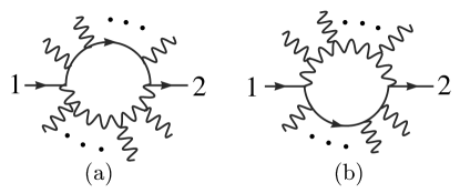
Figure 1: In diagram (a) the fermion line (following the arrow) turns left on entering the loop and is an $L$ type primitive amplitude. In diagram (b) the fermion line turns right and is an $R$ type.

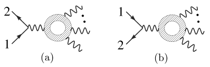
Figure 2: In diagram (a) the external fermion line passes to the “left” of the loop, following the fermion arrow, and is designated an $L$ type. In (b) it passes to the “right” and is an $R$ type. A gluon, fermion or scalar can circulate in the loop. The same decomposition also holds even if we emit additional gluons off the external fermion lines.

As noted above, we can write the one-loop color-ordered amplitudes in the fermionic case more compactly in terms of primitive amplitudes. Each primitive amplitude corresponds to the set of all color-ordered diagrams with specified internal states, and a specified orientation of the fermion line along the loop TwoQuarkThreeGluon .

First consider the case depicted in fig. 1, where the fermion line entering the diagram is part of the loop. Upon entering, the fermion line can turn either “left” and circulate clockwise, or turn “right” and circulate counter-clockwise around the loop. The two orientations correspond to separate primitive amplitudes which we designate as “$L$” and “$R$”. They would carry the same color factor were the fermions in the adjoint representation, but carry different ones when the fermions are in the fundamental representation. This division is therefore gauge invariant. The second case, shown in fig. 2, is where the external fermion line does not enter the loop. This case may also be divided into “left” and “right” pieces, which we again label by “$L$” and “$R$”. Here the division is based on whether the loop passes to the left or right of the fermion line.

The primitive amplitudes for ${\bar{q}}qgg\cdots g$ are,

$$\matrix{&A_{n}^{L,[J]}(1_{\!f},3,4,\ldots,j,2_{\!f},j+1,\ldots,n),\hfill\cr&A_{n}^{R,[J]}(1_{\!f},3,4,\ldots,j,2_{\!f},j+1,\ldots,n),\hfill\cr}\hskip 28.45274ptJ=1,{\textstyle{1\over 2}}\displaystyle,0,$$ (11)

where $J={1\over 2}$ and $J=0$ denote the contributions with a closed fermion loop and closed complex scalar loop, respectively. The second fermion has been placed in the $j^{\rm th}$ position, but assigned the label 2. Since the primitive amplitudes can be used to build amplitudes with any color representation for the fermions, instead of labelling the fermionic legs by $q$ and $\bar{q}$ we label them by $f$ to denote a generic fermion in any color representation. The normalization is such that two helicity states (Weyl fermions or complex scalars) circulate in the loop. Diagrams without closed fermion or scalar loops are assigned to $J=1$; they may or may not contain a closed gluon loop, as the two types of diagrams mix under gauge transformations. For notational simplicity, we shall suppress the superscript “$[1]$”,

$$A_{n}^{L}\equiv A_{n}^{L,[1]}\,,\hskip 56.9055ptA_{n}^{R}\equiv A_{n}^{R,[1]}\,.$$ (12)

The primitive amplitudes (11) are not all independent. The set of diagrams where the incoming leg $1$ turns left is related (up to a sign) to a corresponding set where it turns right. This relation is via a reflection which flips over each diagram, reversing the cyclic ordering:

$$A_{n}^{R,[J]}(1_{\!f},3,4,\ldots,2_{\!f},\ldots,n-1,n)=(-1)^{n}A_{n}^{L,[J]}(1_{\!f},n,n-1,\ldots,2_{\!f},\ldots,4,3).$$ (13)

In addition, the super-Yang-Mills partial amplitudes for two gluinos and $n-2$ gluons $A_{n}^{\rm SUSY}\equiv A_{n;1}^{\rm SUSY}$ are given by the sum (with all cyclic orderings identical)

$$A_{n}^{\rm SUSY}\ \equiv\ A_{n;1}^{\rm SUSY}=A_{n}^{L}\ +\ A_{n}^{R}\ +\ A_{n}^{L,[1/2]}\ +\ A_{n}^{R,[1/2]},$$ (14)

because the “left” and “right” diagrams have the same group-theory weight for an adjoint-representation fermion. Due to supersymmetric cancellations between “left” and “right” primitive amplitudes, $A_{n}^{\rm SUSY}$ is always simpler than either $A_{n}^{L}$ or $A_{n}^{R}$. Equation (14) allows one to obtain one of the four terms on the right with no effort, given $A_{n}^{\rm SUSY}$. In the case of the finite amplitudes we are considering in this paper, $A_{n}^{\rm SUSY}$ vanishes. We will choose to eliminate $A_{n}^{R}$, and compute $A_{n}^{L}$.

Finally, the following fermion-loop contributions vanish,

$$A_{n}^{R,[1/2]}(1_{\!f},2_{\!f},3,4,\ldots,n) = A_{n}^{L,[1/2]}(1_{\!f},n,\ldots,4,3,2_{\!f})=0,$$

$$A_{n}^{R,[1/2]}(1_{\!f},3,2_{\!f},4,\ldots,n) = A_{n}^{L,[1/2]}(1_{\!f},n,\ldots,4,2_{\!f},3)=0,$$ (15)

and similarly for the scalar-loop contributions. The restriction to “left” or “right” diagrams combines with the ordering of the external legs to leave only tadpole and massless external bubble diagrams behind; but these are zero in dimensional regularization.

For scalars and fermions in the fundamental representation circulating in the loop, the leading-color contribution to eq. (2), $A_{n;1}$, is given in terms of primitive amplitudes by,

$$A_{n;1}(1_{\bar{q}},2_{q};3,\ldots,n) = A_{n}^{L}(1_{\!f},2_{\!f},3,\ldots,n)-{1\over N_{c}^{2}}A_{n}^{R}(1_{\!f},2_{\!f},3,\ldots,n)$$ (16)

$$+{n_{\mskip-2.0muf}\over N_{c}}A_{n}^{L,[1/2]}(1_{\!f},2_{\!f},3,\ldots,n)+{n_{\mskip-2.0mus}\over N_{c}}A_{n}^{L,[0]}(1_{\!f},2_{\!f},3,\ldots,n)\,.$$

For QCD the number of scalars vanishes, $n_{\mskip-2.0mus}=0$, while $n_{\mskip-2.0muf}$ is the number of light quark flavors. (Our fundamental representation scalars are normalized so that they carry the same number of states as Dirac fermions, $4N_{c}$.)

As explained in ref. TwoQuarkThreeGluon , the subleading-color partial amplitudes $A_{n;j>1}$ appearing in eq. (2) may be expressed as a permutation sum over primitive amplitudes,

$$\hskip-85.35826ptA_{n;j}(1_{\bar{q}},2_{q};3,\ldots,j+1;j+2,j+3,\ldots,n)$$ (17)

$$= (-1)^{j-1}\sum_{\sigma\in COP\{\alpha\}\{\beta\}}\Biggl{[}A_{n}^{L,[1]}(\sigma(1_{\!f},2_{\!f},3,\ldots,n))$$

$$-{n_{\mskip-2.0muf}\over N_{c}}A_{n}^{R,[1/2]}(\sigma(1_{\!f},2_{\!f},3,\ldots,n))-{n_{\mskip-2.0mus}\over N_{c}}A_{n}^{R,[0]}(\sigma(1_{\!f},2_{\!f},3,\ldots,n))\Biggr{]}\ ,$$

where $\alpha_{i}\in\{\alpha\}\equiv\{j+1,j,\ldots,4,3\}$, $\beta_{i}\in\{\beta\}\equiv\{1,2,j+2,j+3,\ldots,n-1,n\}$, and $COP\{\alpha\}\{\beta\}$ is the set of all permutations of $\{1,2,\ldots,n\}$ with leg $1$ held fixed that preserve the cyclic ordering of the $\alpha_{i}$ within $\{\alpha\}$ and of the $\beta_{i}$ within $\{\beta\}$, while allowing for all possible relative orderings of the $\alpha_{i}$ with respect to the $\beta_{i}$. For example if $\{\alpha\}=\{4,3\}$ and $\{\beta\}=\{1,2,5\}$ (the case required for $A_{5;3}$), then $COP\{\alpha\}\{\beta\}$ contains the twelve elements

$$(1,2,5,4,3),\quad(1,2,4,5,3),\quad(1,4,2,5,3),\quad(1,2,4,3,5),\quad$$

$$(1,4,3,2,5),\quad(1,4,2,3,5),\quad(1,2,5,3,4),\quad(1,2,3,5,4),\quad$$ (18)

$$(1,3,2,5,4),\quad(1,2,3,4,5),\quad(1,3,4,2,5),\quad(1,3,2,4,5).\quad$$

Thus, all partial amplitudes appearing in eq. (2) are expressible as sums over primitive amplitudes and it is sufficient to compute the primitive amplitudes in order to fully specify the complete color-dressed amplitudes.

For the case at hand, where all external gluons carry the same helicity, a supersymmetry identity Susy may be used to prove that the fermion loop and scalar loop are the same up to a sign,

$$A_{n}^{L,[0]}(1_{\!f}^{-},2^{+},\ldots,j_{\!f}^{+},\ldots,n^{+}) = -A_{n}^{L,[1/2]}(1_{\!f}^{-},2^{+},\ldots,j_{\!f}^{+},\ldots,n^{+})$$ (19)

$$\equiv A_{n}^{s}(1_{\!f}^{-},2^{+},\ldots,j_{\!f}^{+},\ldots,n^{+})\,.$$

Thus, by computing the closed scalar-loop primitive amplitude we obtain also the closed fermion-loop primitive amplitude.

We shall find it convenient to compute the combinations

$$A_{n}^{s}\,,\hskip 28.45274pt\hbox{and}\hskip 28.45274ptA_{n}^{L-s}\equiv A_{n}^{L}-A_{n}^{s}\,,$$ (20)

instead of $A_{n}^{s}$ and $A_{n}^{L}$.

Furthermore, combining reflection symmetry and supersymmetry leads to,

$$\hskip-48.36958ptA_{n}^{L}(1_{\!f}^{-},2^{+},\ldots,j_{\!f}^{+},\ldots,n^{+})=(-1)^{n}A_{n}^{R}(1_{\!f}^{-},n^{+},\ldots,j_{\!f}^{+},\ldots,2^{+})$$

$$= (-1)^{n}\Bigl{[}A_{n}^{\rm SUSY}(1_{\!f}^{-},n^{+},\ldots,j_{\!f}^{+},\ldots,2^{+})-A_{n}^{L}(1_{\!f}^{-},n^{+},\ldots,j_{\!f}^{+},\ldots,2^{+})$$

$$\hphantom{=(-1)^{n}\Bigl{[}]}-A_{n}^{L,[1/2]}(1_{\!f}^{-},n^{+},\ldots,j_{\!f}^{+},\ldots,2^{+})-A_{n}^{R,[1/2]}(1_{\!f}^{-},n^{+},\ldots,j_{\!f}^{+},\ldots,2^{+})\Bigr{]}$$

$$= (-1)^{n}\Bigl{[}-A_{n}^{L}(1_{\!f}^{-},n^{+},\ldots,j_{\!f}^{+},\ldots,2^{+})$$

$$\hphantom{=(-1)^{n}\Bigl{[}]}+A_{n}^{L,[0]}(1_{\!f}^{-},n^{+},\ldots,j_{\!f}^{+},\ldots,2^{+})+A_{n}^{R,[0]}(1_{\!f}^{-},n^{+},\ldots,j_{\!f}^{+},\ldots,2^{+})\Bigr{]}$$

$$= (-1)^{n}\Bigl{[}-A_{n}^{L}(1_{\!f}^{-},n^{+},\ldots,j_{\!f}^{+},\ldots,2^{+})$$

$$\hphantom{=(-1)^{n}\Bigl{[}]}+A_{n}^{s}(1_{\!f}^{-},n^{+},\ldots,j_{\!f}^{+},\ldots,2^{+})+(-1)^{n}A_{n}^{s}(1_{\!f}^{-},2^{+},\ldots,j_{\!f}^{+},\ldots,n^{+})\Bigr{]},$$

so that

$$A_{n}^{L-s}(1_{\!f}^{-},2^{+},\ldots,j_{\!f}^{+},\ldots,n^{+})=(-1)^{n+1}A_{n}^{L-s}(1_{\!f}^{-},n^{+},\ldots,j_{\!f}^{+},\ldots,2^{+}),$$ (22)

which we can use to obtain $A_{n}^{L-s}$ for $j>\lceil(n+1)/2\rceil$ ($\lceil x\rceil$ is the smallest integer greater than or equal to $x$). Note also that, as discussed above, $A_{n}^{s}$ vanishes if $j=n$ or $j=n-1$.

In summary, for amplitudes with a single quark pair with identical helicity gluon legs, there are two independent classes of primitive amplitudes that need to be computed,

$$A_{n}^{L-s}(1_{\!f}^{-},2^{+},\ldots,j_{\!f}^{+},\ldots,n^{+})\,,\hskip 28.45274pt\hbox{and}\hskip 28.45274ptA_{n}^{s}(1_{\!f}^{-},2^{+},\ldots,j_{\!f}^{+},\ldots,n^{+})\,.$$ (23)

III Review of Recursion Relations

III.1 On-Shell Recursion Relations for Trees

The on-shell recursion relations rely on general properties of complex functions as well as factorization properties of scattering amplitudes. The proof BCFW of the relations relies on a parameter-dependent shift of two of the external massless spinors, here labelled $k$ and $l$, in an $n$-point process,

$${\tilde{\lambda}}_{k} \rightarrow{\tilde{\lambda}}_{k}-z{\tilde{\lambda}}_{l}\,,$$ (24)

$$\lambda_{l} \rightarrow\lambda_{l}+z\lambda_{k}\,,$$

where $z$ is a complex number. The corresponding momenta (labeled by $p_{i}$ instead of $k_{i}$ in this section) are shifted as well,

$$p_{k}^{\mu} \rightarrow p_{k}^{\mu}(z)=p_{k}^{\mu}-{z\over 2}{\left\langle\smash{k}{\vphantom{1}}^{-}\right|{\gamma^{\mu}}\left|\smash{l}{\vphantom{1}}^{-}\right\rangle},$$ (25)

$$p_{l}^{\mu} \rightarrow p_{l}^{\mu}(z)=p_{l}^{\mu}+{z\over 2}{\left\langle\smash{k}{\vphantom{1}}^{-}\right|{\gamma^{\mu}}\left|\smash{l}{\vphantom{1}}^{-}\right\rangle}\,,$$

so that they remain massless, $p_{k}^{2}(z)=0=p_{l}^{2}(z)$, and overall momentum conservation is maintained. The shift also implies,

$${\raise-1.31944pt\hbox to5.03125pt{\hss/\hss}\hbox to0.0pt{\hss$p$}}_{k} \rightarrow{\raise-1.31944pt\hbox to5.03125pt{\hss/\hss}\hbox to0.0pt{\hss$p$}}_{k}(z)={\raise-1.31944pt\hbox to5.03125pt{\hss/\hss}\hbox to0.0pt{\hss$p$}}_{k}-z\,\bigl{(}\,{|l^{-}\rangle\langle k^{-}|+|k^{+}\rangle\langle l^{+}|}\,\bigr{)}\,,$$ (26)

$${\raise-1.31944pt\hbox to5.03125pt{\hss/\hss}\hbox to0.0pt{\hss$p$}}_{l} \rightarrow{\raise-1.31944pt\hbox to5.03125pt{\hss/\hss}\hbox to0.0pt{\hss$p$}}_{l}(z)={\raise-1.31944pt\hbox to5.03125pt{\hss/\hss}\hbox to0.0pt{\hss$p$}}_{l}+z\,\bigl{(}\,{|l^{-}\rangle\langle k^{-}|+|k^{+}\rangle\langle l^{+}|}\,\bigr{)}\,.$$

Define a parameter-dependent continuation of an on-shell amplitude,

$$A(z)=A(p_{1},\ldots,p_{k}(z),p_{k+1},\ldots,p_{l}(z),\ldots,p_{n}),$$ (27)

evaluated at a particular set of complex momenta. When $A$ is a tree amplitude or finite one-loop amplitude, $A(z)$ is a rational function of $z$. The physical amplitude is given by $A(0)$.

Consider the contour integral,

$${1\over 2\pi i}\oint_{C}{dz\over z}\,A(z)\,,$$ (28)

where the contour is taken around the circle at infinity. If $A(z)\rightarrow 0$ as $z\rightarrow\infty$, as in the tree-level cases BCFRecurrence ; BCFW ; LuoWen ; GravityRecurrence ; BadgerMassive , then there is no “surface term”; that is, the integral (28) vanishes. Evaluating the integral as a sum of residues, we can then solve for $A(0)$ to obtain,

$$A(0)=-\sum_{{\rm poles}\ \alpha}\mathop{\rm Res}_{z=z_{\alpha}}{A(z)\over z}\,.$$ (29)

As explained in ref. BCFW , if $A(z)$ only has simple poles, each residue is given by factorizing the shifted amplitude on the appropriate pole in momentum invariants, so that at tree level,

$$A(0)=\sum_{r,s,h}A^{h}_{L}(z=z_{rs}){i\over K_{r\cdots s}^{2}}A^{-h}_{R}(z=z_{rs})\,,$$ (30)

where $h=\pm 1$ labels the helicity of the intermediate state. There is generically a double sum, labeled by $r,s$, over momentum poles, with legs $k$ and $l$ always appearing on opposite sides of the pole. The squared momentum associated with that pole, $K_{r\cdots s}^{2}$, is evaluated in the unshifted kinematics; whereas the on-shell amplitudes $A_{L}$ and $A_{R}$ are evaluated in kinematics that have been shifted by eq. (24) with $z=z_{rs}$, where

$$z_{rs}=-{K_{r\cdots s}^{2}\over\left\langle\smash{k}{\vphantom{1}}^{-}\right|{{\raise 0.91666pt\hbox to9.20833pt{\hss/\hss}\hbox to0.0pt{\hss$K$}}_{r\ldots s}}\left|\smash{l}{\vphantom{1}}^{-}\right\rangle}\,.$$ (31)

To extend the approach to one loop OnShellRecurrenceI , the sum (30) should also be taken over the two ways of assigning the loop to $A_{L}$ and $A_{R}$. This formula assumes that there are no additional poles present in the amplitude other than the standard poles for real momenta. At tree level it is possible to demonstrate the absence of additional poles, but at loop level it is not true.

For the case of a fermionic pole, there is a sign subtlety similar to the situation with maximally-helicity-violating (MHV) vertices Currents . The correct fermionic propagator is, of course, $i{\raise 0.97221pt\hbox to5.52084pt{\hss/\hss}\hbox to0.0pt{\hss$k$}}/k^{2}$. As is the case for MHV vertices, the /$k$ is supplied by the amplitudes appearing on both sides of the pole. In these amplitudes, each momentum is directed outwards. Thus when we link two amplitudes across the pole we would obtain a numerator factor of the form $|k_{1}^{+}\rangle\langle k_{2}^{+}|$, where $k_{2}=-k_{1}$. This is not quite right since the same momentum argument should appear in both spinors, i.e., $|k_{1}^{+}\rangle\langle k_{1}^{+}|\neq|k_{1}^{+}\rangle\langle(-k_{1})^{+}|$. To correct this we flip the sign of the momentum in the spinor $\langle k_{2}^{+}|$.

Because of the general structure of multiparticle factorization BernChalmers , only standard single poles in $z$ arise from multiparticle channels, even at one loop. However, as was pointed out in ref. OnShellRecurrenceI , double poles in $z$ do arise at one loop due to collinear factorization. The splitting amplitudes with helicity configuration $(+{}+{}+)$ and $(-{}-{}-)$ (in an all-outgoing helicity convention) can lead to double poles in $z$, because their dependence on the spinor products takes the form $\left[a\,b\right]/\left\langle a\,b\right\rangle^{2}$ for $(+{}+{}+)$, or its complex conjugate $\left\langle a\,b\right\rangle/\left[a\,b\right]^{2}$ for $(-{}-{}-)$ Neq4Oneloop . As discussed in ref. OnShellRecurrenceI , this behavior alters the form of the recursion relation in an essential manner. In general, underneath the double pole sits an object of the form,

$${\left[a\,b\right]\over\left\langle a\,b\right\rangle}\,,$$ (32)

which we call an “unreal pole” since there is no pole present when real momenta are used; it only appears, as a single pole, when we continue to complex momenta. As we shall discuss in section V, the finite quark amplitudes exhibit similar phenomena, except that in the quark case we shall also encounter unreal poles not directly associated with a double pole.

III.2 One-loop Factorization Properties

In order to build on-shell recursion relations, we need the factorization properties of one-loop amplitudes for complex momenta. It is useful to first review the factorization properties for real momenta, which we know from general arguments TreeReview ; BernChalmers ; OneloopSplit . Although a good starting point, this is in general insufficient due to the appearance of unreal poles.

As the real momenta of two external legs become collinear, any one-loop amplitude in massless gauge theory will factorize as,

$$A_{n}^{{(1)}}\buildrel a\parallel b\over{\relbar\mskip-0.5mu\joinrel\mskip-0.5mu\relbar\mskip-0.5mu\joinrel\longrightarrow}\ \sum_{\lambda=\pm} \hbox{}\hskip-9.95863pt\biggl{(}\mathop{\rm Split}\nolimits^{(0)}_{-\lambda}(a^{\lambda_{a}},b^{\lambda_{b}};z)\,A_{n-1}^{{(1)}}(\ldots,(a+b)^{\lambda},\ldots)$$ (33)

$$\hphantom{\biggl{(})}+\mathop{\rm Split}\nolimits^{{(1)}}_{-\lambda}(a^{\lambda_{a}},b^{\lambda_{b}};z)\,A_{n-1}^{(0)}(\ldots,(a+b)^{\lambda},\ldots)\biggr{)}\,,$$

where $a$ and $b$ are nearest neighbors in the cyclic ordering of legs. (When they are not nearest neighbors, there is no universal factorization behavior, but also no collinear singularity.) There are three distinct kinds of collinear limits to consider: two gluons becoming collinear; a gluon becoming collinear with a quark (or anti-quark); and a quark and anti-quark becoming collinear (in the case that they are adjacent). These limits simplify in the case at hand, where all external gluons have positive helicity, due to vanishing of relevant $(n-1)$-point tree amplitudes. The required splitting amplitudes are tabulated in ref. Neq4Oneloop .

First consider the case when two cyclically adjacent gluons, $a$ and $b$, become collinear. In this case $A_{n}^{L}$ behaves as,

$$A_{n}^{L}(\ldots,a^{+},b^{+},\ldots)\buildrel a\parallel b\over{\relbar\mskip-0.5mu\joinrel\mskip-0.5mu\relbar\mskip-0.5mu\joinrel\longrightarrow}\ \mathop{\rm Split}\nolimits^{(0)}_{-}(a^{+},b^{+};z)\,A_{n-1}^{L}(\ldots,(a+b)^{+},\ldots)$$ (34)

$$+\mathop{\rm Split}\nolimits^{{(1)}:g}_{+}(a^{+},b^{+};z)\,A_{n-1}^{(0)}(\ldots,(a+b)^{-},\ldots)\,,$$

where $\mathop{\rm Split}\nolimits^{{(1)}:g}$ is the one-loop splitting amplitude with a gluon circulating in the loop. Similarly, $A_{n}^{s}$ behaves as,

$$A_{n}^{s}(\ldots,a^{+},b^{+},\ldots)\buildrel a\parallel b\over{\relbar\mskip-0.5mu\joinrel\mskip-0.5mu\relbar\mskip-0.5mu\joinrel\longrightarrow}\ \mathop{\rm Split}\nolimits^{(0)}_{-}(a^{+},b^{+};z)\,A_{n-1}^{s}(\ldots,(a+b)^{+},\ldots)$$ (35)

$$+\mathop{\rm Split}\nolimits^{{(1)}:s}_{+}(a^{+},b^{+};z)\,A_{n-1}^{(0)}(\ldots,(a+b)^{-},\ldots)\,,$$

where $\mathop{\rm Split}\nolimits^{{(1)}:s}$ is the one-loop splitting amplitude with a scalar circulating in the loop. In both cases, the remaining two terms, with opposite intermediate-gluon helicity, vanish because $\mathop{\rm Split}\nolimits^{(0)}_{+}(a^{+},b^{+};z)$ and $A_{n-1}^{(0)}(\pm,+,+,\ldots,+)$ are zero. Now Neq4Oneloop ,

$$\mathop{\rm Split}\nolimits^{{(1)}:g}_{+}(a^{+},b^{+};z)=\mathop{\rm Split}\nolimits^{{(1)}:s}_{+}(a^{+},b^{+};z),$$ (36)

thanks to a supersymmetry Ward identity Susy . Taking the difference we see that in this limit the $A_{n}^{L-s}$ class of amplitudes to be computed has a very simple structure,

$$A_{n}^{L-s}(\ldots,a^{+},b^{+},\ldots)\buildrel a\parallel b\over{\relbar\mskip-0.5mu\joinrel\mskip-0.5mu\relbar\mskip-0.5mu\joinrel\longrightarrow}\ \mathop{\rm Split}\nolimits^{(0)}_{-}(a^{+},b^{+};z)\,A_{n-1}^{L-s}(\ldots,(a+b)^{+},\ldots)\,.$$ (37)

In the limit that a gluon becomes collinear with the negative-helicity fermion, for either $A_{n}^{L}$ or $A_{n}^{s}$ we find, thanks to helicity conservation on a fermion line, that,

$$A_{n}^{L,s}(a_{\!f}^{-},b^{+},\ldots)\buildrel a\parallel b\over{\relbar\mskip-0.5mu\joinrel\mskip-0.5mu\relbar\mskip-0.5mu\joinrel\longrightarrow}\mathop{\rm Split}\nolimits^{(0)}_{(f)+}(a_{\!f}^{-},b^{+};z)\,A_{n-1}^{L,s}((a+b)_{\!f}^{-},\ldots)\,.$$ (38)

Again taking the difference, we obtain,

$$A_{n}^{L-s}(a_{\!f}^{-},b^{+},\ldots)\buildrel a\parallel b\over{\relbar\mskip-0.5mu\joinrel\mskip-0.5mu\relbar\mskip-0.5mu\joinrel\longrightarrow}\mathop{\rm Split}\nolimits^{(0)}_{(f)+}(a_{\!f}^{-},b^{+};z)\,A_{n-1}^{L-s}((a+b)_{\!f}^{-},\ldots)\,.$$ (39)

A similar expression holds for the limit in which a gluon becomes collinear with the positive-helicity fermion.

Finally, if the quark and anti-quark are adjacent, the amplitude factorizes onto the finite one-loop pure-glue amplitudes,

$$A_{n}^{L,s}(a_{\!f}^{-},b_{\!f}^{+},\ldots)\buildrel a\parallel b\over{\relbar\mskip-0.5mu\joinrel\mskip-0.5mu\relbar\mskip-0.5mu\joinrel\longrightarrow}\ \mathop{\rm Split}\nolimits^{(0)}_{-}(a_{\!f}^{-},b_{\!f}^{+};z)\,A_{n-1}^{{(1)}}((a+b)^{+},\ldots)$$ (40)

$$\hbox{}+\mathop{\rm Split}\nolimits^{(0)}_{+}(a_{\!f}^{-},b_{\!f}^{+};z)\,A_{n-1}^{(1)}((a+b)^{-},\ldots)\,.$$

The gluon and scalar loop contributions to $A_{n-1}^{(1)}(\pm,+,+,\ldots,+)$ are the same by supersymmetry Susy . Hence the difference $A_{n}^{L-s}$ is finite in this limit,

$$A_{n}^{L-s}(a_{\!f}^{-},b_{\!f}^{+},\ldots)\buildrel a\parallel b\over{\relbar\mskip-0.5mu\joinrel\mskip-0.5mu\relbar\mskip-0.5mu\joinrel\longrightarrow}\ \hbox{non-singular}\,.$$ (41)

In the case of multiparticle factorization, the vanishing of $A_{n}^{(0)}(1_{\bar{q}}^{-},2_{q}^{+},3^{+},\ldots,n^{+})$ implies that we can only factorize on a gluon pole,

$$\hbox{}\hskip-11.38109ptA_{n}^{L,s}(1_{\!f}^{-},2^{+},\ldots,j_{\!f}^{+},\ldots,m^{+},\ldots,n^{+})\buildrel K_{1\cdots m}^{2}\rightarrow 0\over{\relbar\mskip-0.5mu\joinrel\mskip-0.5mu\relbar\mskip-0.5mu\joinrel\longrightarrow}$$ (42)

$$\hskip 14.22636ptA_{m+1}^{(0)}(1_{\!f}^{-},2^{+},\ldots,j_{\!f}^{+},\ldots,m^{+},(-K_{1\ldots m})^{-}){i\over K_{1\ldots m}^{2}}A_{n-m+1}^{{(1)}}(K_{1\ldots m}^{+},(m+1)^{+},\ldots,n^{+})\,,$$

with $m\geq 3$. Again $A_{n}^{L-s}$ has a non-singular limit,

$$A_{n}^{L-s}(1_{\!f}^{-},2^{+},\ldots,j_{\!f}^{+},\ldots,m^{+},\ldots,n^{+})\buildrel K_{1\cdots m}^{2}\rightarrow 0\over{\relbar\mskip-0.5mu\joinrel\mskip-0.5mu\relbar\mskip-0.5mu\joinrel\longrightarrow}{\rm non\hbox{-\kern-0.20004pt}{}singular}\,,$$ (43)

since once again the behavior of the $L$ and $s$ pieces are identical and cancel in the $L-s$ difference.

Because of the appearance of unreal poles (32) this is not the entire story. Unfortunately, as yet there are no general theorems to guide us on the factorization properties in this new class of poles. As shown in ref. OnShellRecurrenceI for the finite one-loop pure-glue amplitudes, factorization on the unreal poles is not solely into products of lower-point amplitudes; other factors arise. For the finite quark amplitudes we shall find, just as in ref. OnShellRecurrenceI , a systematic set of correction factors. In section V we will comment on different types of factors that appear.

IV Review of Known Finite QCD amplitudes

In this section, we collect previously-known results for tree and one-loop finite amplitudes, which feed into the recursive formulæ for the finite quark amplitudes to be discussed in section V.

We will need the tree-level MHV amplitudes ParkeTaylor ; TreeReview ,

$$A_{n}^{(0)}(1^{+},2^{+},\ldots,m_{1}^{-},\ldots,m_{2}^{-},\ldots,n^{+})=i{\left\langle m_{1}\,m_{2}\right\rangle^{4}\over\left\langle 1\,2\right\rangle\left\langle 2\,3\right\rangle\cdots\left\langle n\,1\right\rangle}\,,$$ (44)

and

$$A_{n}^{(0)}(1_{\!f}^{-},2^{+},\ldots,j_{\!f}^{+},\ldots,m^{-},\ldots,n^{+})=i{\left\langle 1\,m\right\rangle^{3}\left\langle j\,m\right\rangle\over\left\langle 1\,2\right\rangle\left\langle 2\,3\right\rangle\cdots\left\langle n\,1\right\rangle}\,,$$ (45)

where we use the generic fermion label $f$ again, and where the omitted labels refer to positive-helicity gluons.

We will also need the one-loop pure-gluon amplitudes, either with all helicities positive, or with a single negative helicity. For the all-positive case with $n\geq 4$ legs, Chalmers and the authors AllPlusA ; AllPlus wrote a conjecture  based on collinear limits,

$$A_{n}^{(1)}(1^{+},2^{+},\ldots,n^{+})={i\over 3}{H_{n}\over\left\langle 1\,2\right\rangle\left\langle 2\,3\right\rangle\cdots\left\langle(n-1)\,n\right\rangle\left\langle n\,1\right\rangle}\,,$$ (46)

where

$$H_{n}=-\sum_{1\leq i_{1}<i_{2}<i_{3}<i_{4}\leq n}\,{\rm Tr}_{-}\Bigl{[}{\raise 0.97221pt\hbox to5.52084pt{\hss/\hss}\hbox to0.0pt{\hss$k$}}_{i_{1}}{\raise 0.97221pt\hbox to5.52084pt{\hss/\hss}\hbox to0.0pt{\hss$k$}}_{i_{2}}{\raise 0.97221pt\hbox to5.52084pt{\hss/\hss}\hbox to0.0pt{\hss$k$}}_{i_{3}}{\raise 0.97221pt\hbox to5.52084pt{\hss/\hss}\hbox to0.0pt{\hss$k$}}_{i_{4}}\Bigr{]}\,,$$ (47)

and

$$\,{\rm Tr}_{-}\Bigl{[}{\raise 0.97221pt\hbox to5.52084pt{\hss/\hss}\hbox to0.0pt{\hss$k$}}_{i_{1}}{\raise 0.97221pt\hbox to5.52084pt{\hss/\hss}\hbox to0.0pt{\hss$k$}}_{i_{2}}{\raise 0.97221pt\hbox to5.52084pt{\hss/\hss}\hbox to0.0pt{\hss$k$}}_{i_{3}}{\raise 0.97221pt\hbox to5.52084pt{\hss/\hss}\hbox to0.0pt{\hss$k$}}_{i_{4}}\Bigr{]} = {1\over 2}\,{\rm Tr}[(1-\gamma_{5}){\raise 0.97221pt\hbox to5.52084pt{\hss/\hss}\hbox to0.0pt{\hss$k$}}_{i_{1}}{\raise 0.97221pt\hbox to5.52084pt{\hss/\hss}\hbox to0.0pt{\hss$k$}}_{i_{2}}{\raise 0.97221pt\hbox to5.52084pt{\hss/\hss}\hbox to0.0pt{\hss$k$}}_{i_{3}}{\raise 0.97221pt\hbox to5.52084pt{\hss/\hss}\hbox to0.0pt{\hss$k$}}_{i_{4}}]$$ (48)

$$= \left\langle i_{1}\,i_{2}\right\rangle\left[i_{2}\,i_{3}\right]\left\langle i_{3}\,i_{4}\right\rangle\left[i_{4}\,i_{1}\right]\,.$$

The conjecture was proven by Mahlon Mahlon . In eq. (46) we have extracted an overall factor of $1/(4\pi)^{2}$ compared with ref. AllPlus , to be consistent with the normalization in eq. (2) for the quark amplitudes, and we have set a multiplicity-counting parameter $N_{p}$ to 2, to match the number of color-stripped bosonic states defined to be circulating in the loop in the amplitudes $A_{n}^{s}$. More generally, the overall prefactor $N_{p}$ is just the difference between the number of bosonic and fermionic states circulating in the loop.

For $n=3$ the proper vertex where legs $1$ and $2$ are the external legs is OnShellRecurrenceI ,

$$A_{3}^{(1)}(1^{+},2^{+},3^{+}) = -{i\over 3}{\left[1\,2\right]\left[2\,3\right]\left[3\,1\right]\over K_{12}^{2}}\,.$$ (49)

It is useful to expose the kinematic pole, so we define the vertex,

$$V_{3}^{(1)}(1^{+},2^{+},3^{+})\equiv K_{12}^{2}\,A_{3}^{(1)}(1^{+},2^{+},3^{+})=-{i\over 3}\left[1\,2\right]\left[2\,3\right]\left[3\,1\right]\,.$$ (50)

The single negative-helicity amplitudes may also be required as inputs into the quark recursion relation. The four-point amplitude was first calculated using string-based methods and is given by BKStringBased ,

$$A_{4}^{(1)}(1^{-},2^{+},3^{+},4^{+}) = {i\over 3}\,{\left\langle 2\,4\right\rangle\left[2\,4\right]^{3}\over\left[1\,2\right]\left\langle 2\,3\right\rangle\left\langle 3\,4\right\rangle\left[4\,1\right]}\,.$$ (51)

The five-point amplitude with a single negative-helicity leg was also first calculated using string-based methods and is given by GGGGG ; AllPlusA ,

$$A_{5}^{(1)}(1^{-},2^{+},3^{+},4^{+},5^{+})={i\over 3}\,{1\over\left\langle 3\,4\right\rangle^{2}}\Biggl{[}-{\left[2\,5\right]^{3}\over\left[1\,2\right]\left[5\,1\right]}+{\left\langle 1\,4\right\rangle^{3}\left[4\,5\right]\left\langle 3\,5\right\rangle\over\left\langle 1\,2\right\rangle\left\langle 2\,3\right\rangle\left\langle 4\,5\right\rangle^{2}}-{\left\langle 1\,3\right\rangle^{3}\left[3\,2\right]\left\langle 4\,2\right\rangle\over\left\langle 1\,5\right\rangle\left\langle 5\,4\right\rangle\left\langle 3\,2\right\rangle^{2}}\Biggr{]}\,.$$ (52)

The $n$-point generalization was then obtained by Mahlon Mahlon via off-shell recursive methods. We recently used an on-shell recursion relation to obtain compact representations of the six- and seven-point amplitudes OnShellRecurrenceI . The six-point amplitude is,

$$A_{6}^{(1)}(1^{-},2^{+},3^{+},4^{+},5^{+},6^{+})$$

$$\hskip 14.22636pt={i\over 3}\,\Biggl{[}{{\left\langle\smash{1}{\vphantom{1}}^{-}\right|{(2+3)}\left|\smash{6}{\vphantom{1}}^{-}\right\rangle}^{3}\over\left\langle 1\,2\right\rangle\left\langle 2\,3\right\rangle{\left\langle 4\,5\right\rangle}^{2}\,s_{123}\,\left\langle\smash{3}{\vphantom{1}}^{-}\right|{(1+2)}\left|\smash{6}{\vphantom{1}}^{-}\right\rangle}\hbox{}+{{\left\langle\smash{1}{\vphantom{1}}^{-}\right|{(3+4)}\left|\smash{2}{\vphantom{1}}^{-}\right\rangle}^{3}\over{\left\langle 3\,4\right\rangle}^{2}\left\langle 5\,6\right\rangle\left\langle 6\,1\right\rangle\,s_{234}\,\left\langle\smash{5}{\vphantom{1}}^{-}\right|{(3+4)}\left|\smash{2}{\vphantom{1}}^{-}\right\rangle}$$

$$\hskip 56.9055pt\hbox{}+{{\left[2\,6\right]}^{3}\over\left[1\,2\right]\left[6\,1\right]\,s_{345}}\Biggl{(}{\left[2\,3\right]\left[3\,4\right]\over\left\langle 4\,5\right\rangle\,\left\langle\smash{5}{\vphantom{1}}^{-}\right|{(3+4)}\left|\smash{2}{\vphantom{1}}^{-}\right\rangle}-{\left[4\,5\right]\left[5\,6\right]\over\left\langle 3\,4\right\rangle\,\left\langle\smash{3}{\vphantom{1}}^{-}\right|{(1+2)}\left|\smash{6}{\vphantom{1}}^{-}\right\rangle}+{\left[3\,5\right]\over\left\langle 3\,4\right\rangle\left\langle 4\,5\right\rangle}\Biggr{)}$$

$$\hskip 56.9055pt\hbox{}-{{\left\langle 1\,3\right\rangle}^{3}\left[2\,3\right]\left\langle 2\,4\right\rangle\over{\left\langle 2\,3\right\rangle}^{2}{\left\langle 3\,4\right\rangle}^{2}\left\langle 4\,5\right\rangle\left\langle 5\,6\right\rangle\left\langle 6\,1\right\rangle}+{{\left\langle 1\,5\right\rangle}^{3}\left\langle 4\,6\right\rangle\left[5\,6\right]\over\left\langle 1\,2\right\rangle\left\langle 2\,3\right\rangle\left\langle 3\,4\right\rangle{\left\langle 4\,5\right\rangle}^{2}{\left\langle 5\,6\right\rangle}^{2}}$$

$$\hskip 56.9055pt-{{\left\langle 1\,4\right\rangle}^{3}\left\langle 3\,5\right\rangle\left\langle\smash{1}{\vphantom{1}}^{-}\right|{(2+3)}\left|\smash{4}{\vphantom{1}}^{-}\right\rangle\over\left\langle 1\,2\right\rangle\left\langle 2\,3\right\rangle{\left\langle 3\,4\right\rangle}^{2}{\left\langle 4\,5\right\rangle}^{2}\left\langle 5\,6\right\rangle\left\langle 6\,1\right\rangle}\Biggr{]}\,.$$ (53)

In section V, we give a compact expression for all $n$.

The known results for the fermionic four-point amplitudes KunsztEtAl are,

$$A_{4}^{L-s}(1_{\!f}^{-},2_{\!f}^{+},3^{+},4^{+}) = -{i\over 2}{\left\langle 1\,2\right\rangle\left[2\,4\right]\over\left\langle 2\,3\right\rangle\left\langle 3\,4\right\rangle}\,,$$

$$A_{4}^{s}(1_{\!f}^{-},2_{\!f}^{+},3^{+},4^{+}) = -{i\over 3}{\left\langle 1\,4\right\rangle\left[2\,4\right]\over\left\langle 3\,4\right\rangle^{2}}\,,$$ (54)

and for the five-point fermionic amplitudes TwoQuarkThreeGluon ,

$$A_{5}^{L-s}(1_{\!f}^{-},2_{\!f}^{+},3^{+},4^{+},5^{+}) = {i\over 2}{\left\langle 1\,2\right\rangle\left[2\,3\right]\left\langle 3\,1\right\rangle+\left\langle 1\,4\right\rangle\left[4\,5\right]\left\langle 5\,1\right\rangle\over\left\langle 2\,3\right\rangle\left\langle 3\,4\right\rangle\left\langle 4\,5\right\rangle\left\langle 5\,1\right\rangle}\,,$$

$$A_{5}^{s}(1_{\!f}^{-},2_{\!f}^{+},3^{+},4^{+},5^{+}) = -{i\over 3}\Biggl{(}{\left\langle 1\,3\right\rangle\left[3\,4\right]\left\langle 4\,1\right\rangle^{2}\over\left\langle 1\,2\right\rangle\left\langle 3\,4\right\rangle^{2}\left\langle 4\,5\right\rangle\left\langle 5\,1\right\rangle}+{\left\langle 1\,4\right\rangle\left\langle 2\,4\right\rangle\left[4\,5\right]\left\langle 5\,1\right\rangle\over\left\langle 1\,2\right\rangle\left\langle 2\,3\right\rangle\left\langle 3\,4\right\rangle\left\langle 4\,5\right\rangle^{2}}$$

$$\hskip 28.45274pt+{\left[2\,3\right]\left[2\,5\right]\over\left[1\,2\right]\left\langle 3\,4\right\rangle\left\langle 4\,5\right\rangle}\Biggr{)}\,,$$

$$A_{5}^{L-s}(1_{\!f}^{-},2^{+},3_{\!f}^{+},4^{+},5^{+}) = {i\over 2}{\left\langle 1\,3\right\rangle(\left\langle 1\,2\right\rangle\left[2\,3\right]\left\langle 3\,1\right\rangle+\left\langle 1\,4\right\rangle\left[4\,5\right]\left\langle 5\,1\right\rangle)\over\left\langle 1\,2\right\rangle\left\langle 2\,3\right\rangle\left\langle 3\,4\right\rangle\left\langle 4\,5\right\rangle\left\langle 5\,1\right\rangle}\,,$$

$$A_{5}^{s}(1_{\!f}^{-},2^{+},3_{\!f}^{+},4^{+},5^{+}) = {i\over 3}{\left\langle 1\,4\right\rangle\left\langle 1\,5\right\rangle\left[4\,5\right]\over\left\langle 1\,2\right\rangle\left\langle 2\,3\right\rangle\left\langle 4\,5\right\rangle^{2}}\,.$$ (55)

V Quark Recursion Relations

As was discussed in section II, for the finite helicity amplitudes — one quark pair, with all gluons having positive helicity — there are two independent primitive amplitudes that need to be computed,

$$A_{n}^{L-s}(j_{\!f}^{+}) \equiv A_{n}^{L-s}(1_{\!f}^{-},2^{+},\ldots,j_{\!f}^{+},\ldots,n^{+})\,,\qquad 2\leq j\leq\lceil(n+1)/2\rceil\,,$$ (56)

$$A_{n}^{s}(j_{\!f}^{+}) \equiv A_{n}^{s}(1_{\!f}^{-},2^{+},\ldots,j_{\!f}^{+},\ldots,n^{+})\,,\qquad 2\leq j\leq n-2\,,$$ (57)

where we have adopted an abbreviated notation retaining only the label of the positive-helicity fermion. A computation of these primitive amplitudes then determines all the finite one-loop quark amplitudes in QCD.

V.1 Structure of Five-Point Recursion for $L-s$ Contribution

Let us begin, as in ref. OnShellRecurrenceI , by examining the structure of five point amplitudes. Consider $A_{5}^{L-s}(2_{\!f}^{+})$, as defined in eq. (56), and choosing $(k,l)=(1,5)$ as shift variables in eq. (24),

$$\lambda_{1} \rightarrow \lambda_{1}\,,$$

$${\tilde{\lambda}}_{1} \rightarrow {\tilde{\lambda}}_{1}-z{\tilde{\lambda}}_{5}\,,$$

$$\lambda_{5} \rightarrow \lambda_{5}+z\lambda_{1}\,,$$ (58)

$${\tilde{\lambda}}_{5} \rightarrow {\tilde{\lambda}}_{5}\,,$$

with all other spinors unchanged. Under this shift, using the known result for the amplitude we have

$$A_{5}^{L-s}(2_{\!f}^{+};z)={i\over 2}{\left\langle 1\,2\right\rangle\left\langle 1\,3\right\rangle\left[2\,3\right]\over\left\langle 2\,3\right\rangle\left\langle 3\,4\right\rangle(\left\langle 4\,5\right\rangle+z\left\langle 4\,1\right\rangle)\left\langle 1\,5\right\rangle}+{i\over 2}{\left\langle 1\,4\right\rangle\left[4\,5\right]\over\left\langle 2\,3\right\rangle\left\langle 3\,4\right\rangle(\left\langle 4\,5\right\rangle+z\left\langle 4\,1\right\rangle)}\,.$$ (59)

which vanishes as $z\rightarrow\infty$, so no surface term is required. Looking at the $z=0$ pole in $A_{5}^{L-s}(z)/z$, we expect to find the following two terms,

$${i\over 2}{\left\langle 1\,2\right\rangle\left\langle 1\,3\right\rangle\left[2\,3\right]\over\left\langle 2\,3\right\rangle\left\langle 3\,4\right\rangle\left\langle 4\,5\right\rangle\left\langle 1\,5\right\rangle}+{i\over 2}{\left\langle 1\,4\right\rangle\left[4\,5\right]\over\left\langle 2\,3\right\rangle\left\langle 3\,4\right\rangle\left\langle 4\,5\right\rangle}\,,$$ (60)

appearing in the recursion.

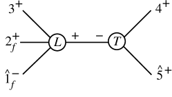
Figure 3: The real-pole diagram in the recursion relation for $A_{5}^{L-s}(1_{\!f}^{+},2_{\!f}^{+},3^{+},4^{+},5^{+})$. The vertices labeled by a $T$ are trees, and the ones labeled by an $L$ are loops.

On the other hand, from the structure of the collinear limits — eqs. (37), (39), and (41) — we expect to find only one term. A lone term, displayed in fig. 3, is indeed what emerges from the naive form of the recursion relation,

$$D_{1} = {i\over s_{45}}A_{4}^{L-s}(\hat{1}_{\!f}^{-},2_{\!f}^{+},3^{+},{\hat{K}}_{45}^{+})A_{3}^{(0)}((-{\hat{K}}_{45})^{-},4^{+},\hat{5}^{+})$$

$$= -{i\over 2}{1\over s_{45}}{\vphantom{\hat{K}}\left\langle\smash{\hat{1}}\,\smash{2}\right\rangle\vphantom{\hat{K}}\left[\smash{2}\,\smash{{\hat{K}}_{45}}\right]\over\left\langle 2\,3\right\rangle\vphantom{\hat{K}}\left\langle\smash{3}\,\smash{{\hat{K}}_{45}}\right\rangle}{\vphantom{\hat{K}}\left[\smash{4}\,\smash{\hat{5}}\right]^{3}\over\vphantom{\hat{K}}\left[\smash{(-{\hat{K}}_{45})}\,\smash{4}\right]\vphantom{\hat{K}}\left[\smash{\hat{5}}\,\smash{(-{\hat{K}}_{45})}\right]}$$

$$= {i\over 2}{1\over s_{45}}{\left\langle 1\,2\right\rangle\left\langle\smash{1}{\vphantom{1}}^{-}\right|{{\raise 0.91666pt\hbox to9.20833pt{\hss/\hss}\hbox to0.0pt{\hss$K$}}_{45}}\left|\smash{2}{\vphantom{1}}^{-}\right\rangle\over\left\langle 2\,3\right\rangle\left\langle\smash{3}{\vphantom{1}}^{-}\right|{{\raise 0.91666pt\hbox to9.20833pt{\hss/\hss}\hbox to0.0pt{\hss$K$}}_{45}}\left|\smash{5}{\vphantom{1}}^{-}\right\rangle}{\left[4\,5\right]^{3}\over\left\langle\smash{1}{\vphantom{1}}^{-}\right|{{\raise 0.91666pt\hbox to9.20833pt{\hss/\hss}\hbox to0.0pt{\hss$K$}}_{45}}\left|\smash{4}{\vphantom{1}}^{-}\right\rangle}$$

$$= {i\over 2}{1\over s_{45}}{\left\langle 1\,2\right\rangle\left\langle 1\,3\right\rangle\left[3\,2\right]\over\left\langle 2\,3\right\rangle\left\langle 3\,4\right\rangle\left[4\,5\right]}{{\left[4\,5\right]}^{2}\over\left\langle 1\,5\right\rangle}$$

$$= {i\over 2}{\left\langle 1\,2\right\rangle\left\langle 1\,3\right\rangle\left[2\,3\right]\over\left\langle 2\,3\right\rangle\left\langle 3\,4\right\rangle\left\langle 4\,5\right\rangle\left\langle 1\,5\right\rangle}\,,$$

exactly the first term in $A_{5}^{L-s}$. But the second term in eq. (60) is missing.

What happened to it? Notice that the second term in eq. (60) is not singular in the $k_{4}\parallel k_{5}$ limit, so long as we are considering real momenta, because the numerator and denominator vanish at the same rate in the limit. If we consider complex momenta, however, the behavior of $\left\langle 4\,5\right\rangle$ is decoupled from that of $\left[4\,5\right]$, and in regions where $\left\langle 4\,5\right\rangle\rightarrow 0$, there is a pole.

In other words: while multiparticle and collinear factorization capture the full pole structure for real momenta, they do not do so for complex momenta. In particular, a term containing the unreal pole (32) in the $a\parallel b$ limit, will not contribute to a collinear singularity, but will contribute to a pole for complex momenta (which decouple the behavior of $\left\langle a\,b\right\rangle$ from that of $\left[a\,b\right]$). That is, for our purposes we need to ask what the quasi-universal behavior in the collinear limit is of finite terms with non-trivial phase structure. For real momenta the ratio (32) is always nonsingular, because $|\left\langle a\,b\right\rangle|=|\left[a\,b\right]|=\sqrt{|2k_{a}\cdot k_{b}|}$. (It does contain a phase dependence, though, which selects it out uniquely in the collinear limit: as the vectors $\vec{k}_{a}$ and $\vec{k}_{b}$ are rotated around each other by an angle $\phi$ the ratio (32) will change by the phase factor $\exp(-2i\phi)$.)

Figure 4: The extra unreal pole contribution in the recursion relation for $A_{5}^{L-s}(1_{\!f}^{+},2_{\!f}^{+},3^{+},4^{+},5^{+})$.

At tree level, a diagrammatic analysis that isolates the collinear singularities for real momenta extends readily (for massless amplitudes) to complex momenta. However, the same is not true at loop level. We will not offer such an analysis in this paper. Rather, we will exhibit a set of ansätze which use lower-point amplitudes and yield the contributions required for the corresponding poles.

We proceed as in ref. OnShellRecurrenceI . Our experience there suggests that the missing term is associated with a factorization of the type shown in fig. 4. In order to define the 3-point loop vertex in this diagram, we could try to use the factor $V_{3}^{{(1)}}$ vertex (50) which appeared in the gluonic case OnShellRecurrenceI . However, eq. (60) contains a normalization factor of $1/2$ rather than $1/3$, and is not associated directly with a double pole. So we introduce the “$L\!-\!s$ loop vertex”,

$$V_{3}^{L-s}(1^{+},2^{+},3^{+})\equiv-{i\over 2}\left[1\,2\right]\left[2\,3\right]\left[3\,1\right]\,,$$ (62)

which is proportional to $V_{3}^{{(1)}}$.

In the present case, there is no real-pole contribution associated with the diagram in fig. 4; it would correspond to an “$A^{s\,}$” contribution which we have subtracted out in $A^{L-s}$. (Accordingly, for complex momenta, the double pole contributions present in ref. OnShellRecurrenceI are absent.) However, unreal pole contributions can arise. There are a number of constraints that allow us to find the precise form of the required term. The unreal pole is power-suppressed by a factor of $s_{45}$ compared to the diagram in fig. 4. By dimensional analysis we then need additional factors to obtain the correct overall dimensions. The additional factors must be invariant under phase rotations of spinors associated with all external states, and the intermediate state $\hat{K}_{45}$.

We can use universal multiplicative “soft factors,” which describe the insertion of a soft gluon $s$ between two hard partons $a$ and $b$ in a color-ordered amplitude, to construct such a multiplicative function. The soft factors depend only on the helicity of the soft gluon and are given by TreeReview ,

$${\cal S}^{(0)}(a,s^{+},b) = {\left\langle a\,b\right\rangle\over\left\langle a\,s\right\rangle\left\langle s\,b\right\rangle}\,,$$ (63)

$${\cal S}^{(0)}(a,s^{-},b) = -{\left[a\,b\right]\over\left[a\,s\right]\left[s\,b\right]}\,.$$ (64)

They are invariant under phase rotations of spinors associated with $a$ and $b$, but not $s$. However, the product

$$s_{45}{\cal S}^{(0)}(a,s^{+},b){\cal S}^{(0)}(c,(-s)^{-},d)$$ (65)

is dimensionless, invariant under phase rotations of $a$, $b$, $c$, $d$ and $s$, and suppressed as $K_{45}^{2}\to 0$, for suitable choices of $a$, $b$, $c$, $d$ and $s$.

Since the leg $s$ appears in two factors in eq. (65) carrying opposite helicity, it is natural to identify it with the on-shell intermediate momentum $\hat{K}_{45}$. Choosing $c=\hat{5}$ and $d=4$ produces the desired collinear behavior $\propto\left\langle 4\,5\right\rangle$ for eq. (65). A little experimentation shows that here the legs $2$ and $\hat{1}$ should be identified with $a$ and $b$. Multiplying eq. (65) with these assignments by the “naive” diagram in fig. 4,

$${i\over s_{45}^{2}}A_{4}^{(0)}(\hat{1}_{\!f}^{-},2_{\!f}^{+},3^{+},{\hat{K}}_{45}^{-})\,V_{3}^{L-s}((-{\hat{K}}_{45})^{+},4^{+},\hat{5}^{+})\,,$$ (66)

gives us exactly the missing contribution,

$${i\over 2}{\left\langle 1\,4\right\rangle\left[4\,5\right]\over\left\langle 2\,3\right\rangle\left\langle 3\,4\right\rangle\left\langle 4\,5\right\rangle}\,.$$ (67)

More generally, in the $n$-point on-shell recursion relation for $A_{n}^{L-s}(j_{\!f}^{+})$, when we choose the shifted legs in eq. (24) to be $(k,l)=(1,n)$, we need to add an unreal-pole term of the form,

$${i\over s_{(n-1)n}}A_{n-1}^{(0)}(\hat{1}_{\!f}^{-},2^{+},\ldots,j_{\!f}^{+},\ldots,(n-2)^{+},{\hat{K}}_{(n-1)n}^{-})V_{3}^{L-s}((-{\hat{K}}_{(n-1)n})^{+},(n-1)^{+},\hat{n}^{+})$$

$$\hskip 42.67912pt\hbox{}\times{\cal S}^{(0)}(j,{\hat{K}}_{(n-1)n}^{+},\hat{1})\,{\cal S}^{(0)}(\hat{n},(-{\hat{K}}_{(n-1)n})^{-},n-1)\,.$$ (68)

The complete recursion relation for this choice of shifted legs is then,

$$\hbox{}\hskip-28.45274ptA_{n}^{L-s}(j_{\!f}^{+})$$ (69)

$$= {i\over s_{(n-1)n}}A_{n-1}^{L-s}(\hat{1}_{\!f}^{-},2^{+},\ldots,j_{\!f}^{+},\ldots,(n-2)^{+},{\hat{K}}_{(n-1)n}^{+})A_{3}^{{(0)}}((-{\hat{K}}_{(n-1)n})^{-},(n-1)^{+},\hat{n}^{+})$$

$$\hskip 5.69054pt\hbox{}+{i\over s_{(n-1)n}}A_{n-1}^{(0)}(\hat{1}_{\!f}^{-},2^{+},\ldots,j_{\!f}^{+},\ldots,(n-2)^{+},{\hat{K}}_{(n-1)n}^{-})V_{3}^{L-s}((-{\hat{K}}_{(n-1)n})^{+},(n-1)^{+},\hat{n}^{+})$$

$$\hskip 56.9055pt\hbox{}\times{\cal S}^{(0)}(j,{\hat{K}}_{(n-1)n}^{+},\hat{1})\,{\cal S}^{(0)}(\hat{n},(-{\hat{K}}_{(n-1)n})^{-},n-1)\,,$$

where the hatted momenta in eq. (69) are defined by the shift

$${\tilde{\lambda}}_{1} \rightarrow{\tilde{\lambda}}_{1}-z{\tilde{\lambda}}_{n}\,,$$ (70)

$$\lambda_{n} \rightarrow\lambda_{n}+z\lambda_{1}\,,$$

with

$$z=-{K_{n-1,n}^{2}\over\left\langle\smash{1}{\vphantom{1}}^{-}\right|{{\raise 0.91666pt\hbox to9.20833pt{\hss/\hss}\hbox to0.0pt{\hss$K$}}_{n-1,n}}\left|\smash{n}{\vphantom{1}}^{-}\right\rangle}=-{\left\langle(n-1)\,n\right\rangle\over\left\langle(n-1)\,1\right\rangle}\,,$$ (71)

in each term. This relation assumes that, as in the case $n=5$, the shifted amplitude $A(z)$ vanishes as $z\rightarrow\infty$, so there is no surface term to be added to eq. (29). The recursion relation (69) can be solved, yielding the following simple expression,

$$A_{n}^{L-s}(1_{\!f}^{-},2^{+},\ldots,j_{\!f}^{+},\ldots,n^{+})={i\over 2}{\left\langle 1\,j\right\rangle\Sigma_{l=3}^{n-1}\left\langle\smash{1}{\vphantom{1}}^{-}\right|{{\raise 0.91666pt\hbox to9.20833pt{\hss/\hss}\hbox to0.0pt{\hss$K$}}_{2\cdots l}{\raise 0.97221pt\hbox to5.52084pt{\hss/\hss}\hbox to0.0pt{\hss$k$}}_{l}}\left|\smash{1}{\vphantom{1}}^{+}\right\rangle\over\left\langle 1\,2\right\rangle\left\langle 2\,3\right\rangle\cdots\left\langle n\,1\right\rangle}\,.$$ (72)

The reader may verify that this result has the correct collinear limits in all channels, and that it obeys the reflection symmetry (22).

V.2 Structure of Recursion for $s$ Contribution

We turn next to the computation of the scalar contributions, given by the $A_{n}^{s}$ function. In this case, there is a non-trivial collinear limit when $k_{n-1}\parallel k_{n}$ with real momenta, so that we expect to have both double-pole and single-pole contributions with complex momenta. The latter may have an interpretation as ‘underlying’ the double-pole term, or else as simply being unreal poles. The presence of both types of term is similar to the gluon amplitudes with one negative-helicity gluon considered in ref. OnShellRecurrenceI . We can again find an appropriate function using soft factors; the factors here are however different from those in the gluon case. As above, take the shifts to be $(1,n)$. In the five-point case, for example, the factors are,

$${\cal S}^{(0)}(3,{\hat{K}}_{45}^{+},2)\,{\cal S}^{(0)}(\hat{5},(-{\hat{K}}_{45})^{-},4)\,,$$ (73)

when the positive-helicity quark is leg $2$, and absent if it is leg $3$. This observation suggests a general form,

$${\cal S}^{(0)}(n-2,{\hat{K}}_{(n-1)n}^{+},j)\,{\cal S}^{(0)}(\hat{n},(-{\hat{K}}_{(n-1)n})^{-},n-1)\,,$$ (74)

where $j$ labels the positive-helicity quark.

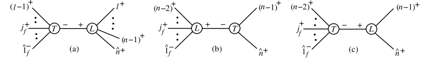
Figure 5: The diagrams corresponding to the terms in the recursion relation in eq. (75). In diagram (a) $l$ runs over $\{j+1,j+2,\ldots,n-2\}$. Diagram (c) contains a double pole as well as an unreal pole underneath it.

The full recursion relation for $A_{n}^{s}(j_{\!f}^{+})$, again assuming the absence of a $z\rightarrow\infty$ surface term, is depicted in fig. 5, and reads,

$$\hbox{}\hskip-14.22636ptA_{n}^{s}(j_{\!f}^{+})$$

$$=\sum_{l=j+1}^{n-2}{i\over s_{l\ldots n}}A_{l}^{(0)}(1_{\!f}^{-},2^{+},\ldots,j_{\!f}^{+},\ldots,(l-1)^{+},{\hat{K}}_{l\ldots n}^{-})A_{n-l+2}^{{(1)}}((-{\hat{K}}_{l\ldots n})^{+},l^{+},\ldots,\hat{n}^{+})$$

$$\hbox{}+{i\over s_{(n-1)n}}A_{n-1}^{s}(\hat{1}_{\!f}^{-},2^{+},\ldots,j_{\!f}^{+},\ldots,(n-2)^{+},{\hat{K}}_{(n-1)n}^{+})A_{3}^{{(0)}}((-{\hat{K}}_{(n-1)n})^{-},(n-1)^{+},\hat{n}^{+})$$

$$\hbox{}+{i\over s_{(n-1)n}^{2}}A_{n-1}^{(0)}(\hat{1}_{\!f}^{-},2^{+},\ldots,j_{\!f}^{+},\ldots,(n-2)^{+},{\hat{K}}_{(n-1)n}^{-})V_{3}^{{(1)}}((-{\hat{K}}_{(n-1)n})^{+},(n-1)^{+},\hat{n}^{+})$$

$$\hskip 14.22636pt\hbox{}\times\Bigl{(}1+s_{(n-1)n}\,{\cal S}^{(0)}(n-2,{\hat{K}}_{(n-1)n}^{+},j)\,{\cal S}^{(0)}(\hat{n},(-{\hat{K}}_{(n-1)n})^{-},n-1)\Bigr{)}\,.$$ (75)

The hatted legs undergo the shift in eq. (70), where in the $s_{l\ldots n}$ channel we set,

$$z=-{s_{l\ldots n}\over\left\langle\smash{1}{\vphantom{1}}^{-}\right|{{\raise 0.91666pt\hbox to9.20833pt{\hss/\hss}\hbox to0.0pt{\hss$K$}}_{l\ldots n}}\left|\smash{n}{\vphantom{1}}^{-}\right\rangle}\,.$$ (76)

The tree-side soft factor here, ${\cal S}^{(0)}(n-2,{\hat{K}}_{(n-1)n}^{+},j)$, is in a sense the “complement” of that for $A_{n}^{L-s}$ appearing in eq. (68); that is,

$${\cal S}^{(0)}(n-2,{\hat{K}}_{(n-1)n}^{+},j)+{\cal S}^{(0)}(j,{\hat{K}}_{(n-1)n}^{+},\hat{1})={\cal S}^{(0)}(n-2,{\hat{K}}_{(n-1)n}^{+},\hat{1})\,,$$ (77)

where the right-hand side is exactly the tree-side soft factor that appeared in our previous recursion relation OnShellRecurrenceI for the one-loop all-gluon amplitude with one negative helicity.

V.3 Solution to $A_{n}^{s}$ Recursion Relation

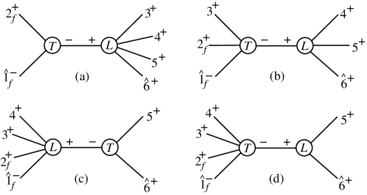
Figure 6: The recursive diagrams for $A_{6}^{s}(2_{\!f}^{+})$ using the shift in eq. (70) with $n=6$.

Unlike $A_{n}^{L-s}$, $A_{n}^{s}$ does have multi-particle poles. Consider the six-point case. If we use the shift (70) the recursion relation (75) generates the diagrams shown in fig. 6 for the case where leg 2 is the positive helicity fermion leg. The other cases, where the positive-helicity fermion is leg 3 or 4, are similar. Evaluating these contributions, we find,

$$A_{6}^{s}(2_{\!f}^{+}) = {i\over 3}\Biggl{(}{\left\langle 1\,4\right\rangle\left\langle\smash{1}{\vphantom{1}}^{-}\right|{(2+3)(3+4)}\left|\smash{1}{\vphantom{1}}^{+}\right\rangle\over\left\langle 1\,2\right\rangle{\left\langle 3\,4\right\rangle}^{2}\left\langle 4\,5\right\rangle\left\langle 5\,6\right\rangle\left\langle 6\,1\right\rangle}+{\left\langle 2\,4\right\rangle\left\langle 1\,5\right\rangle\left\langle\smash{1}{\vphantom{1}}^{-}\right|{(4+5)(5+6)}\left|\smash{1}{\vphantom{1}}^{+}\right\rangle\over\left\langle 1\,2\right\rangle\left\langle 2\,3\right\rangle\left\langle 3\,4\right\rangle{\left\langle 4\,5\right\rangle}^{2}\left\langle 5\,6\right\rangle\left\langle 6\,1\right\rangle}\hskip 42.67912pt$$ (78)

$$\hskip 14.22636pt-{\left\langle 2\,5\right\rangle\left\langle\smash{1}{\vphantom{1}}^{-}\right|{5\,6}\left|\smash{1}{\vphantom{1}}^{+}\right\rangle\over\left\langle 1\,2\right\rangle\left\langle 2\,3\right\rangle\left\langle 3\,4\right\rangle\left\langle 4\,5\right\rangle{\left\langle 5\,6\right\rangle}^{2}}+{{\left\langle\smash{1}{\vphantom{1}}^{-}\right|{(3+4)}\left|\smash{2}{\vphantom{1}}^{-}\right\rangle}^{2}\over{\left\langle 3\,4\right\rangle}^{2}\left\langle 5\,6\right\rangle\left\langle 6\,1\right\rangle\left\langle\smash{5}{\vphantom{1}}^{-}\right|{(3+4)}\left|\smash{2}{\vphantom{1}}^{-}\right\rangle}$$

$$\hskip 14.22636pt-{\left[2\,6\right]^{2}\left\langle\smash{2}{\vphantom{1}}^{+}\right|{(3+4)(4+5)(3+4)(4+5)}\left|\smash{6}{\vphantom{1}}^{-}\right\rangle\over\left[1\,2\right]\left\langle 3\,4\right\rangle\left\langle 4\,5\right\rangle\left\langle\smash{5}{\vphantom{1}}^{-}\right|{(3+4)}\left|\smash{2}{\vphantom{1}}^{-}\right\rangle\left\langle\smash{3}{\vphantom{1}}^{-}\right|{(4+5)}\left|\smash{6}{\vphantom{1}}^{-}\right\rangle s_{345}}$$

$$\hskip 14.22636pt+{\left\langle\smash{2}{\vphantom{1}}^{-}\right|{(4+5)}\left|\smash{6}{\vphantom{1}}^{-}\right\rangle{\left\langle\smash{1}{\vphantom{1}}^{-}\right|{(4+5)}\left|\smash{6}{\vphantom{1}}^{-}\right\rangle}^{2}\over\left\langle 1\,2\right\rangle\left\langle 2\,3\right\rangle{\left\langle 4\,5\right\rangle}^{2}\left\langle\smash{3}{\vphantom{1}}^{-}\right|{(4+5)}\left|\smash{6}{\vphantom{1}}^{-}\right\rangle s_{456}}\Biggr{)}\,,$$

$$A_{6}^{s}(3_{\!f}^{+}) = {i\over 3}\Biggl{(}{\left\langle 1\,5\right\rangle\left\langle 1\,6\right\rangle\left\langle 3\,5\right\rangle\left[5\,6\right]\over\left\langle 1\,2\right\rangle\left\langle 2\,3\right\rangle\left\langle 3\,4\right\rangle\left\langle 4\,5\right\rangle\left\langle 5\,6\right\rangle^{2}}+{\left\langle 1\,5\right\rangle\left\langle\smash{1}{\vphantom{1}}^{-}\right|{(4+5)(5+6)}\left|\smash{1}{\vphantom{1}}^{+}\right\rangle\over\left\langle 1\,2\right\rangle\left\langle 2\,3\right\rangle\left\langle 4\,5\right\rangle^{2}\left\langle 5\,6\right\rangle\left\langle 6\,1\right\rangle}$$ (79)

$$\hskip 14.22636pt+{\left\langle\smash{1}{\vphantom{1}}^{-}\right|{(4+5)}\left|\smash{6}{\vphantom{1}}^{-}\right\rangle^{2}\over\left\langle 1\,2\right\rangle\left\langle 2\,3\right\rangle\left\langle 4\,5\right\rangle^{2}s_{123}}\Biggr{)},$$

$$A_{6}^{s}(4_{\!f}^{+}) = -{i\over 3}{\left\langle\smash{1}{\vphantom{1}}^{-}\right|{5\,6}\left|\smash{1}{\vphantom{1}}^{+}\right\rangle\over\left\langle 1\,2\right\rangle\left\langle 2\,3\right\rangle\left\langle 3\,4\right\rangle\left\langle 5\,6\right\rangle^{2}}\,.$$ (80)

These expressions suggest the all-$n$ forms,

$$A_{n}^{s}((n-2)_{\!f}^{+}) = -{i\over 3}{\left\langle\smash{1}{\vphantom{1}}^{-}\right|{(n-1)\,n}\left|\smash{1}{\vphantom{1}}^{+}\right\rangle\over\left\langle 1\,2\right\rangle\cdots\left\langle(n-3)\,(n-2)\right\rangle\left\langle(n-1)\,n\right\rangle^{2}},~{}~{}~{}~{}~{}$$ (81)

$$A_{n}^{s}((n-3)_{\!f}^{+}) = {i\over 3}\Biggl{(}-{\left\langle\smash{1}{\vphantom{1}}^{-}\right|{(n-1)\,n}\left|\smash{1}{\vphantom{1}}^{+}\right\rangle\left\langle(n-3)\,(n-1)\right\rangle\over\left\langle 1\,2\right\rangle\left\langle 2\,3\right\rangle\cdots\left\langle(n-2)\,(n-1)\right\rangle\left\langle(n-1)\,n\right\rangle^{2}}$$ (82)

$$\hphantom{{i\over 3}\Biggl{(})\!}+{\left\langle 1\,(n-1)\right\rangle\left\langle\smash{1}{\vphantom{1}}^{-}\right|{{\raise 0.91666pt\hbox to9.20833pt{\hss/\hss}\hbox to0.0pt{\hss$K$}}_{n-2,n-1}{\raise 0.91666pt\hbox to9.20833pt{\hss/\hss}\hbox to0.0pt{\hss$K$}}_{n-1,n}}\left|\smash{1}{\vphantom{1}}^{+}\right\rangle\over\left\langle 1\,2\right\rangle\left\langle 2\,3\right\rangle\cdots\left\langle(n-4)\,(n-3)\right\rangle\left\langle(n-2)\,(n-1)\right\rangle^{2}\left\langle(n-1)\,n\right\rangle\left\langle n\,1\right\rangle}$$

$$\hphantom{{i\over 3}\Biggl{(})\!}+{\left\langle\smash{1}{\vphantom{1}}^{-}\right|{{\raise 0.91666pt\hbox to9.20833pt{\hss/\hss}\hbox to0.0pt{\hss$K$}}_{n-2,n-1}}\left|\smash{n}{\vphantom{1}}^{-}\right\rangle^{2}\over\left\langle 1\,2\right\rangle\left\langle 2\,3\right\rangle\cdots\left\langle(n-4)\,(n-3)\right\rangle\left\langle(n-2)\,(n-1)\right\rangle^{2}s_{(n-2)\cdots n}}\Biggr{)}\,.$$

By studying the structure of eqs. (78)–(82), and also the output of the recursion relation for $n=7$ and $n=8$, we have arrived at the following compact formula, valid for all $j$ and $n$,

$$A_{n}^{s}(j_{\!f}^{+})={i\over 3}{S_{1}+S_{2}\over\left\langle 1\,2\right\rangle\left\langle 2\,3\right\rangle\cdots\left\langle n\,1\right\rangle}\,,$$ (83)

where

$$S_{1} = \sum_{l=j+1}^{n-1}{\left\langle j\,l\right\rangle\left\langle 1\,(l+1)\right\rangle\left\langle\smash{1}{\vphantom{1}}^{-}\right|{{\raise 0.91666pt\hbox to9.20833pt{\hss/\hss}\hbox to0.0pt{\hss$K$}}_{l,l+1}{\raise 0.91666pt\hbox to9.20833pt{\hss/\hss}\hbox to0.0pt{\hss$K$}}_{(l+1)\cdots n}}\left|\smash{1}{\vphantom{1}}^{+}\right\rangle\over\left\langle l\,(l+1)\right\rangle}\,,$$ (84)

$$S_{2} = \sum_{l=j+1}^{n-2}\sum_{p=l+1}^{n-1}{\left\langle(l-1)\,l\right\rangle\over\left\langle\smash{1}{\vphantom{1}}^{-}\right|{{\raise 0.91666pt\hbox to9.20833pt{\hss/\hss}\hbox to0.0pt{\hss$K$}}_{(p+1)\cdots n}{\raise 0.91666pt\hbox to9.20833pt{\hss/\hss}\hbox to0.0pt{\hss$K$}}_{l\cdots p}}\left|\smash{(l-1)}{\vphantom{1}}^{+}\right\rangle\left\langle\smash{1}{\vphantom{1}}^{-}\right|{{\raise 0.91666pt\hbox to9.20833pt{\hss/\hss}\hbox to0.0pt{\hss$K$}}_{(p+1)\cdots n}{\raise 0.91666pt\hbox to9.20833pt{\hss/\hss}\hbox to0.0pt{\hss$K$}}_{l\cdots p}}\left|\smash{l}{\vphantom{1}}^{+}\right\rangle}$$ (85)

$$\hskip 42.67912pt\times{\left\langle p\,(p+1)\right\rangle\over\left\langle\smash{1}{\vphantom{1}}^{-}\right|{{\raise 0.91666pt\hbox to9.20833pt{\hss/\hss}\hbox to0.0pt{\hss$K$}}_{2\cdots(l-1)}{\raise 0.91666pt\hbox to9.20833pt{\hss/\hss}\hbox to0.0pt{\hss$K$}}_{l\cdots p}}\left|\smash{p}{\vphantom{1}}^{+}\right\rangle\left\langle\smash{1}{\vphantom{1}}^{-}\right|{{\raise 0.91666pt\hbox to9.20833pt{\hss/\hss}\hbox to0.0pt{\hss$K$}}_{2\cdots(l-1)}{\raise 0.91666pt\hbox to9.20833pt{\hss/\hss}\hbox to0.0pt{\hss$K$}}_{l\cdots p}}\left|\smash{(p+1)}{\vphantom{1}}^{+}\right\rangle}$$

$$\hskip 42.67912pt\times{\left\langle\smash{1}{\vphantom{1}}^{-}\right|{{\raise 0.91666pt\hbox to9.20833pt{\hss/\hss}\hbox to0.0pt{\hss$K$}}_{l\cdots p}{\raise 0.91666pt\hbox to9.20833pt{\hss/\hss}\hbox to0.0pt{\hss$K$}}_{(p+1)\cdots n}}\left|\smash{1}{\vphantom{1}}^{+}\right\rangle}^{2}\left\langle\smash{j}{\vphantom{1}}^{-}\right|{{\raise 0.91666pt\hbox to9.20833pt{\hss/\hss}\hbox to0.0pt{\hss$K$}}_{l\cdots p}{\raise 0.91666pt\hbox to9.20833pt{\hss/\hss}\hbox to0.0pt{\hss$K$}}_{(p+1)\cdots n}}\left|\smash{1}{\vphantom{1}}^{+}\right\rangle$$

$$\hskip 42.67912pt\times{\left\langle\smash{1}{\vphantom{1}}^{-}\right|{{\raise 0.91666pt\hbox to9.20833pt{\hss/\hss}\hbox to0.0pt{\hss$K$}}_{2\cdots(l-1)}[{\cal F}(l,p)]^{2}{\raise 0.91666pt\hbox to9.20833pt{\hss/\hss}\hbox to0.0pt{\hss$K$}}_{(p+1)\cdots n}}\left|\smash{1}{\vphantom{1}}^{+}\right\rangle\over s_{l\cdots p}}\,,$$

and

$${\cal F}(l,p)=\sum_{i=l}^{p-1}\sum_{m=i+1}^{p}{\raise 0.97221pt\hbox to5.52084pt{\hss/\hss}\hbox to0.0pt{\hss$k$}}_{i}{\raise 0.97221pt\hbox to5.52084pt{\hss/\hss}\hbox to0.0pt{\hss$k$}}_{m}\,.$$ (86)

V.4 Verification of Solution

We now verify analytically that these amplitudes satisfy the recursion relation (75). First consider the term shown in fig. 5(b), containing the three-point tree amplitude $A_{3}^{{(0)}}((-{\hat{K}}_{(n-1)n})^{-},(n-1)^{+},\hat{n}^{+})$. Let $\hat{S}_{1}$ and $\hat{S}_{2}$ stand for the shifted versions of $S_{1}$ and $S_{2}$ for the appropriate $(n-1)$-point one-loop quark amplitude. The term in fig. 5(b) can be simplified to

$$-{1\over K_{n-1,n}^{2}}{{\left[(n-1)\,n\right]}^{3}\over\vphantom{\hat{K}}\left[\smash{n}\,\smash{\hat{K}_{n-1,n}}\right]\vphantom{\hat{K}}\left[\smash{\hat{K}_{n-1,n}}\,\smash{(n-1)}\right]}$$ (87)

$$\hskip 34.1433pt\times{i\over 3}{\hat{S}_{1}+\hat{S}_{2}\over\vphantom{\hat{K}}\left\langle\smash{\hat{K}_{n-1,n}}\,\smash{1}\right\rangle\left\langle 1\,2\right\rangle\left\langle 2\,3\right\rangle\cdots\left\langle(n-3)\,(n-2)\right\rangle\vphantom{\hat{K}}\left\langle\smash{(n-2)}\,\smash{\hat{K}_{n-1,n}}\right\rangle}$$

$$= {i\over 3}{\hat{S}_{1}+\hat{S}_{2}\over\left\langle 1\,2\right\rangle\left\langle 2\,3\right\rangle\cdots\left\langle n\,1\right\rangle}{\left\langle(n-2)\,(n-1)\right\rangle\left\langle(n-1)\,n\right\rangle\left\langle n\,1\right\rangle{\left[(n-1)\,n\right]}^{3}\over\left\langle(n-1)\,n\right\rangle\left[(n-1)\,n\right]\left\langle\smash{1}{\vphantom{1}}^{-}\right|{{\raise 0.91666pt\hbox to9.20833pt{\hss/\hss}\hbox to0.0pt{\hss$K$}}_{n-1,n}}\left|\smash{(n-1)}{\vphantom{1}}^{-}\right\rangle\left\langle\smash{(n-2)}{\vphantom{1}}^{-}\right|{{\raise 0.91666pt\hbox to9.20833pt{\hss/\hss}\hbox to0.0pt{\hss$K$}}_{n-1,n}}\left|\smash{n}{\vphantom{1}}^{-}\right\rangle}$$

$$= {i\over 3}{\hat{S}_{1}+\hat{S}_{2}\over\left\langle 1\,2\right\rangle\left\langle 2\,3\right\rangle\cdots\left\langle n\,1\right\rangle}\,.$$

We see that the correct spinor denominator factor is reproduced.

The next question is how $\hat{S}_{1}$ and $\hat{S}_{2}$ are affected by the shift (70). Because $\hat{S}_{1}$ is simpler, we discuss it first. Note that the $(n-1)$-point expression $\hat{S}_{1}$ is a single sum over $l$ containing $(n-2)-j$ terms, which is one fewer than the number of terms in the $n$-point expression $S_{1}$ we are trying to produce. All terms but the last in $\hat{S}_{1}$ have very simple behavior under the shift (70) of ${\tilde{\lambda}}_{1}$ and $\lambda_{n}$. They depend on $\lambda_{1}$ through $\langle 1^{-}|$ and $|1^{+}\rangle$, but do not depend on ${\tilde{\lambda}}_{1}$. Their dependence on $\lambda_{n}$ is solely via the factor

$$\ldots({\raise 0.91666pt\hbox to9.20833pt{\hss/\hss}\hbox to0.0pt{\hss$K$}}_{(l+1)\cdots(n-2)}+\hat{{\raise 0.91666pt\hbox to9.20833pt{\hss/\hss}\hbox to0.0pt{\hss$K$}}}_{n-1,n})|1^{+}\rangle=\ldots{\raise 0.91666pt\hbox to9.20833pt{\hss/\hss}\hbox to0.0pt{\hss$K$}}_{(l+1)\cdots n}|1^{+}\rangle\,,$$ (88)

because the shift in ${\raise 0.91666pt\hbox to9.20833pt{\hss/\hss}\hbox to0.0pt{\hss$K$}}_{n-1,n}$ is proportional to $\lambda_{1}$. Thus each such term directly yields the corresponding term in the $n$-point sum $S_{1}$.

The last term in $\hat{S}_{1}$, with $l=n-2$, is the exception, because it has additional dependence on ${\raise 0.91666pt\hbox to9.20833pt{\hss/\hss}\hbox to0.0pt{\hss$K$}}_{n-1,n}$. It can be written as

$${\left\langle j\,(n-2)\right\rangle\vphantom{\hat{K}}\left\langle\smash{1}\,\smash{\hat{K}_{n-1,n}}\right\rangle\vphantom{\hat{K}}\left[\smash{\hat{K}_{n-1,n}}\,\smash{n}\right]\left\langle\smash{1}{\vphantom{1}}^{-}\right|{({\raise 0.97221pt\hbox to5.52084pt{\hss/\hss}\hbox to0.0pt{\hss$k$}}_{n-2}+{\raise 0.91666pt\hbox to9.20833pt{\hss/\hss}\hbox to0.0pt{\hss$K$}}_{n-1,n}){\raise 0.91666pt\hbox to9.20833pt{\hss/\hss}\hbox to0.0pt{\hss$K$}}_{n-1,n}}\left|\smash{1}{\vphantom{1}}^{+}\right\rangle\over\vphantom{\hat{K}}\left\langle\smash{(n-2)}\,\smash{\hat{K}_{n-1,n}}\right\rangle\vphantom{\hat{K}}\left[\smash{\hat{K}_{n-1,n}}\,\smash{n}\right]}$$ (89)

$$= {\left\langle j\,(n-2)\right\rangle\left\langle 1\,{(n-1)}\right\rangle\left\langle\smash{1}{\vphantom{1}}^{-}\right|{{\raise 0.97221pt\hbox to5.52084pt{\hss/\hss}\hbox to0.0pt{\hss$k$}}_{n-2}{\raise 0.91666pt\hbox to9.20833pt{\hss/\hss}\hbox to0.0pt{\hss$K$}}_{n-1,n}}\left|\smash{1}{\vphantom{1}}^{+}\right\rangle\over\left\langle(n-2)\,(n-1)\right\rangle}\,,$$

which does not quite match the next-to-last term ($l=n-2$) in $S_{1}$,

$${\left\langle j\,(n-2)\right\rangle\left\langle 1\,{(n-1)}\right\rangle\left\langle\smash{1}{\vphantom{1}}^{-}\right|{{\raise 0.91666pt\hbox to9.20833pt{\hss/\hss}\hbox to0.0pt{\hss$K$}}_{n-2,n-1}{\raise 0.91666pt\hbox to9.20833pt{\hss/\hss}\hbox to0.0pt{\hss$K$}}_{n-1,n}}\left|\smash{1}{\vphantom{1}}^{+}\right\rangle\over\left\langle(n-2)\,(n-1)\right\rangle}\,.$$ (90)

Additional contributions to the next-to-last term, and the whole of the last term ($l=n-1$) in $S_{1}$, come from the term containing $V_{3}^{{(1)}}((-{\hat{K}}_{(n-1)n})^{+},(n-1)^{+},\hat{n}^{+})$ in the recursion relation (75), depicted in fig. 5(c). This term can be simplified to,

$${i\over 3}{1\over s_{(n-1)n}^{2}}{{\vphantom{\hat{K}}\left\langle\smash{1}\,\smash{\hat{K}_{n-1,n}}\right\rangle}^{2}\vphantom{\hat{K}}\left\langle\smash{j}\,\smash{\hat{K}_{n-1,n}}\right\rangle\vphantom{\hat{K}}\left[\smash{\hat{K}_{n-1,n}}\,\smash{(n-1)}\right]\left[(n-1)\,n\right]\vphantom{\hat{K}}\left[\smash{n}\,\smash{\hat{K}_{n-1,n}}\right]\over\left\langle 1\,2\right\rangle\left\langle 2\,3\right\rangle\cdots\left\langle(n-3)\,(n-2)\right\rangle\vphantom{\hat{K}}\left\langle\smash{(n-2)}\,\smash{\hat{K}_{n-1,n}}\right\rangle}$$ (91)

$$\hskip 19.91692pt\times\Biggl{(}1+s_{(n-1)n}{\left\langle(n-2)\,j\right\rangle\left[n\,(n-1)\right]\over\vphantom{\hat{K}}\left\langle\smash{(n-2)}\,\smash{\hat{K}_{n-1,n}}\right\rangle\vphantom{\hat{K}}\left\langle\smash{\hat{K}_{n-1,n}}\,\smash{j}\right\rangle\vphantom{\hat{K}}\left[\smash{n}\,\smash{\hat{K}_{n-1,n}}\right]\vphantom{\hat{K}}\left[\smash{\hat{K}_{n-1,n}}\,\smash{(n-1)}\right]}\Biggr{)}$$

$$= -{i\over 3}{1\over\left\langle 1\,2\right\rangle\left\langle 2\,3\right\rangle\cdots\left\langle(n-3)\,(n-2)\right\rangle}$$

$$\hskip 19.91692pt\times{\left\langle\smash{1}{\vphantom{1}}^{-}\right|{{\raise 0.91666pt\hbox to9.20833pt{\hss/\hss}\hbox to0.0pt{\hss$K$}}_{n-1,n}}\left|\smash{(n-1)}{\vphantom{1}}^{-}\right\rangle\left\langle\smash{1}{\vphantom{1}}^{-}\right|{{\raise 0.91666pt\hbox to9.20833pt{\hss/\hss}\hbox to0.0pt{\hss$K$}}_{n-1,n}}\left|\smash{n}{\vphantom{1}}^{-}\right\rangle\left\langle\smash{j}{\vphantom{1}}^{-}\right|{{\raise 0.91666pt\hbox to9.20833pt{\hss/\hss}\hbox to0.0pt{\hss$K$}}_{n-1,n}}\left|\smash{n}{\vphantom{1}}^{-}\right\rangle\left[(n-1)\,n\right]\over{\left\langle(n-1)\,n\right\rangle}^{2}{\left[(n-1)\,n\right]}^{2}\left\langle\smash{(n-2)}{\vphantom{1}}^{-}\right|{{\raise 0.91666pt\hbox to9.20833pt{\hss/\hss}\hbox to0.0pt{\hss$K$}}_{n-1,n}}\left|\smash{n}{\vphantom{1}}^{-}\right\rangle}$$

$$\hskip 19.91692pt\times\Biggl{(}1-{\left\langle j\,(n-2)\right\rangle\left\langle(n-1)\,n\right\rangle{\left[(n-1)\,n\right]}^{2}\left\langle\smash{1}{\vphantom{1}}^{-}\right|{{\raise 0.91666pt\hbox to9.20833pt{\hss/\hss}\hbox to0.0pt{\hss$K$}}_{n-1,n}}\left|\smash{n}{\vphantom{1}}^{-}\right\rangle\over\left\langle\smash{(n-2)}{\vphantom{1}}^{-}\right|{{\raise 0.91666pt\hbox to9.20833pt{\hss/\hss}\hbox to0.0pt{\hss$K$}}_{n-1,n}}\left|\smash{n}{\vphantom{1}}^{-}\right\rangle\left\langle\smash{j}{\vphantom{1}}^{-}\right|{{\raise 0.91666pt\hbox to9.20833pt{\hss/\hss}\hbox to0.0pt{\hss$K$}}_{n-1,n}}\left|\smash{n}{\vphantom{1}}^{-}\right\rangle\left\langle\smash{1}{\vphantom{1}}^{-}\right|{{\raise 0.91666pt\hbox to9.20833pt{\hss/\hss}\hbox to0.0pt{\hss$K$}}_{n-1,n}}\left|\smash{(n-1)}{\vphantom{1}}^{-}\right\rangle}\Biggr{)}$$

$$= {i\over 3}{1\over\left\langle 1\,2\right\rangle\left\langle 2\,3\right\rangle\cdots\left\langle n\,1\right\rangle}{\left\langle j\,(n-1)\right\rangle\left\langle 1\,n\right\rangle\left\langle\smash{1}{\vphantom{1}}^{-}\right|{{\raise 0.91666pt\hbox to9.20833pt{\hss/\hss}\hbox to0.0pt{\hss$K$}}_{n-1,n}{\raise 0.97221pt\hbox to5.52084pt{\hss/\hss}\hbox to0.0pt{\hss$k$}}_{n}}\left|\smash{1}{\vphantom{1}}^{+}\right\rangle\over\left\langle(n-1)\,n\right\rangle}$$

$$\hskip 19.91692pt\times\Biggl{(}1+{\left\langle j\,(n-2)\right\rangle\left\langle(n-1)\,n\right\rangle\left\langle 1\,(n-1)\right\rangle\over\left\langle j\,(n-1)\right\rangle\left\langle(n-2)\,(n-1)\right\rangle\left\langle 1\,n\right\rangle}\Biggr{)}$$

$$= {i\over 3}{1\over\left\langle 1\,2\right\rangle\left\langle 2\,3\right\rangle\cdots\left\langle n\,1\right\rangle}\Biggl{(}{\left\langle j\,(n-1)\right\rangle\left\langle 1\,n\right\rangle\left\langle\smash{1}{\vphantom{1}}^{-}\right|{{\raise 0.91666pt\hbox to9.20833pt{\hss/\hss}\hbox to0.0pt{\hss$K$}}_{n-1,n}{\raise 0.97221pt\hbox to5.52084pt{\hss/\hss}\hbox to0.0pt{\hss$k$}}_{n}}\left|\smash{1}{\vphantom{1}}^{+}\right\rangle\over\left\langle(n-1)\,n\right\rangle}$$

$$\hskip 102.42992pt+{\left\langle j\,(n-2)\right\rangle\left\langle 1\,(n-1)\right\rangle\left\langle\smash{1}{\vphantom{1}}^{-}\right|{{\raise 0.97221pt\hbox to5.52084pt{\hss/\hss}\hbox to0.0pt{\hss$k$}}_{n-1}{\raise 0.91666pt\hbox to9.20833pt{\hss/\hss}\hbox to0.0pt{\hss$K$}}_{n-1,n}}\left|\smash{1}{\vphantom{1}}^{+}\right\rangle\over\left\langle(n-2)\,(n-1)\right\rangle}\Biggr{)}\,.$$

The term containing $\left\langle j\,(n-2)\right\rangle$ in eq. (91) combines with eq. (89) to generate the next-to-last term (90) in $S_{1}$, while the term containing $\left\langle j\,(n-1)\right\rangle$ is just the last term in $S_{1}$. So we have demonstrated that all of the terms in $S_{1}$ are produced correctly by the recursion relation.

Now we turn to $S_{2}$. We divide the $S_{2}$ terms into those with $p<n-1$ and those with $p=n-1$. The bulk of the terms, with $p<n-1$, come from the $\hat{S}_{2}$ contribution we left unexamined in eq. (87). To show this, we observe that (as was the case for the bulk of the $\hat{S}_{1}$ terms) ${\tilde{\lambda}}_{1}$ never appears in $\hat{S}_{2}$. Also, $k_{n}$ only appears in eq. (85) for $S_{2}$ via $\langle 1^{-}|{\raise 0.91666pt\hbox to9.20833pt{\hss/\hss}\hbox to0.0pt{\hss$K$}}_{(p+1)\cdots n}\ldots$ or $\ldots{\raise 0.91666pt\hbox to9.20833pt{\hss/\hss}\hbox to0.0pt{\hss$K$}}_{(p+1)\cdots n}|1^{+}\rangle$. Thus we may again apply eq. (88) (with $l$ replaced by $p$) to $\hat{S}_{2}$, in order to see that every term with $p<n-1$ in $S_{2}$ is generated directly from the corresponding term in $\hat{S}_{2}$.

The $S_{2}$ terms with $p=n-1$ come from the terms containing the one-loop pure-glue all-plus amplitude $A_{n-l+2}^{{(1)}}$ in eq. (75), depicted in fig. 5(a). The $l^{\rm th}$ term in $S_{2}$ comes from the $l^{\rm th}$ term in the recursion relation. The main technical detail is to rewrite the numerator $H_{n}$ of the all-plus amplitude, as given in eq. (47), so that it looks like the operator $[{\cal F}(l,n-1)]^{2}$ appearing in the terms with $p=n-1$ in $S_{2}$. For this purpose, we first use the identity (122), with $p=n$, to rewrite the numerator factor $H_{n-l+2}(l,n)$ (for the all-plus amplitude with gluon momenta $k_{l},k_{l+1},\ldots,k_{n},P$, where $P=-K_{l\cdots n}$ is on-shell) as,

$$H_{n-l+2}(l,n)=-{1\over 2}\,{\rm Tr}_{-}[{\cal F}(l,n)]^{2}\,.$$ (92)

Then we use the identity

$${1\over 2}\,{\rm Tr}_{-}[{\cal F}(l,n)]^{2}={\langle n^{+}|\,[\hat{{\cal F}}(l,n)]^{2}\,|\hat{K}_{l\cdots n}^{-}\rangle\over\vphantom{\hat{K}}\left[\smash{n}\,\smash{\hat{K}_{l\cdots n}}\right]}\,,$$ (93)

where $\hat{{\cal F}}$ is defined in eq. (116), which follows similarly from eqs. (121) and (115) for $p=n$. Finally, eq. (130) shows that we can shift $n\to n-1$ in the argument of $\hat{{\cal F}}$ in eq. (93). Combining this equation with eq. (92), reversing the order of the spinor strings, using momentum conservation, and multiplying numerator and denominator by common factors, we arrive at the identity,

$$H_{n-l+2}(l,n)=-{\left\langle\smash{1}{\vphantom{1}}^{-}\right|{{\raise 0.91666pt\hbox to9.20833pt{\hss/\hss}\hbox to0.0pt{\hss$K$}}_{2\cdots(l-1)}[{\cal F}(l,n-1)]^{2}{\raise 0.97221pt\hbox to5.52084pt{\hss/\hss}\hbox to0.0pt{\hss$k$}}_{n}}\left|\smash{1}{\vphantom{1}}^{+}\right\rangle\over\left\langle\smash{1}{\vphantom{1}}^{-}\right|{{\raise 0.91666pt\hbox to9.20833pt{\hss/\hss}\hbox to0.0pt{\hss$K$}}_{2\cdots(l-1)}{\raise 0.97221pt\hbox to5.52084pt{\hss/\hss}\hbox to0.0pt{\hss$k$}}_{n}}\left|\smash{1}{\vphantom{1}}^{+}\right\rangle}\,.$$ (94)

A few other identities are also useful,

$$\left\langle n\,1\right\rangle\,s_{l\cdots n} = \left\langle\smash{1}{\vphantom{1}}^{-}\right|{{\raise 0.91666pt\hbox to9.20833pt{\hss/\hss}\hbox to0.0pt{\hss$K$}}_{2\cdots(l-1)}{\raise 0.91666pt\hbox to9.20833pt{\hss/\hss}\hbox to0.0pt{\hss$K$}}_{l\cdots(n-1)}}\left|\smash{n}{\vphantom{1}}^{+}\right\rangle\,,$$ (95)

$$\left\langle\smash{\hat{n}}{\vphantom{1}}^{-}\right|{{\raise 0.91666pt\hbox to9.20833pt{\hss/\hss}\hbox to0.0pt{\hss$K$}}_{l\cdots n}}\left|\smash{n}{\vphantom{1}}^{-}\right\rangle = \left\langle\smash{n}{\vphantom{1}}^{-}\right|{{\raise 0.91666pt\hbox to9.20833pt{\hss/\hss}\hbox to0.0pt{\hss$K$}}_{l\cdots n}}\left|\smash{n}{\vphantom{1}}^{-}\right\rangle-{K^{2}_{l\cdots n}\over\left\langle\smash{1}{\vphantom{1}}^{-}\right|{{\raise 0.91666pt\hbox to9.20833pt{\hss/\hss}\hbox to0.0pt{\hss$K$}}_{l\cdots n}}\left|\smash{n}{\vphantom{1}}^{-}\right\rangle}\left\langle\smash{1}{\vphantom{1}}^{-}\right|{{\raise 0.91666pt\hbox to9.20833pt{\hss/\hss}\hbox to0.0pt{\hss$K$}}_{l\cdots n}}\left|\smash{n}{\vphantom{1}}^{-}\right\rangle$$ (96)

$$= -s_{l\cdots(n-1)}\,,$$

$$\left\langle(n-1)\,\hat{n}\right\rangle = \left\langle(n-1)\,n\right\rangle-{K^{2}_{l\cdots n}\over\left\langle\smash{1}{\vphantom{1}}^{-}\right|{{\raise 0.91666pt\hbox to9.20833pt{\hss/\hss}\hbox to0.0pt{\hss$K$}}_{l\cdots n}}\left|\smash{n}{\vphantom{1}}^{-}\right\rangle}\left\langle(n-1)\,1\right\rangle$$ (97)

$$= -{\left\langle\smash{1}{\vphantom{1}}^{-}\right|{{\raise 0.91666pt\hbox to9.20833pt{\hss/\hss}\hbox to0.0pt{\hss$K$}}_{2\cdots(l-1)}{\raise 0.91666pt\hbox to9.20833pt{\hss/\hss}\hbox to0.0pt{\hss$K$}}_{l\cdots(n-1)}}\left|\smash{{(n-1)}}{\vphantom{1}}^{+}\right\rangle\over\left\langle\smash{1}{\vphantom{1}}^{-}\right|{{\raise 0.91666pt\hbox to9.20833pt{\hss/\hss}\hbox to0.0pt{\hss$K$}}_{l\cdots n}}\left|\smash{n}{\vphantom{1}}^{-}\right\rangle}\,.$$

Using these identities, the $l^{\rm th}$ term in the recursion relation can be written as,

$$-{i\over 3}{1\over s_{l\cdots n}}{{\vphantom{\hat{K}}\left\langle\smash{1}\,\smash{\hat{K}_{l\cdots n}}\right\rangle}^{2}\vphantom{\hat{K}}\left\langle\smash{j}\,\smash{\hat{K}_{l\cdots n}}\right\rangle\over\left\langle 1\,2\right\rangle\left\langle 2\,3\right\rangle\cdots\left\langle(l-2)\,(l-1)\right\rangle\vphantom{\hat{K}}\left\langle\smash{(l-1)}\,\smash{\hat{K}_{l\cdots n}}\right\rangle}$$ (98)

$$\hskip 28.45274pt\hbox{}\times{H_{n-l+2}(l,n)\over\vphantom{\hat{K}}\left\langle\smash{\hat{K}_{l\cdots n}}\,\smash{l}\right\rangle\left\langle l\,(l+1)\right\rangle\cdots\left\langle(n-1)\,\hat{n}\right\rangle\vphantom{\hat{K}}\left\langle\smash{\hat{n}}\,\smash{\hat{K}_{l\cdots n}}\right\rangle}$$

$$= -{i\over 3}{1\over\left\langle 1\,2\right\rangle\left\langle 2\,3\right\rangle\cdots\left\langle n\,1\right\rangle}{\left\langle(l-1)\,l\right\rangle\left\langle(n-1)\,n\right\rangle\left\langle n\,1\right\rangle{\left\langle\smash{1}{\vphantom{1}}^{-}\right|{{\raise 0.91666pt\hbox to9.20833pt{\hss/\hss}\hbox to0.0pt{\hss$K$}}_{l\cdots n}}\left|\smash{n}{\vphantom{1}}^{-}\right\rangle}^{2}\left\langle\smash{j}{\vphantom{1}}^{-}\right|{{\raise 0.91666pt\hbox to9.20833pt{\hss/\hss}\hbox to0.0pt{\hss$K$}}_{l\cdots n}}\left|\smash{n}{\vphantom{1}}^{-}\right\rangle\over\left\langle\smash{n}{\vphantom{1}}^{+}\right|{{\raise 0.91666pt\hbox to9.20833pt{\hss/\hss}\hbox to0.0pt{\hss$K$}}_{l\cdots n}}\left|\smash{(l-1)}{\vphantom{1}}^{+}\right\rangle\left\langle\smash{n}{\vphantom{1}}^{+}\right|{{\raise 0.91666pt\hbox to9.20833pt{\hss/\hss}\hbox to0.0pt{\hss$K$}}_{l\cdots n}}\left|\smash{l}{\vphantom{1}}^{+}\right\rangle}$$

$$\hskip 28.45274pt\hbox{}\times{\left\langle n\,1\right\rangle\over\left\langle\smash{1}{\vphantom{1}}^{-}\right|{{\raise 0.91666pt\hbox to9.20833pt{\hss/\hss}\hbox to0.0pt{\hss$K$}}_{2\cdots(l-1)}{\raise 0.91666pt\hbox to9.20833pt{\hss/\hss}\hbox to0.0pt{\hss$K$}}_{l\cdots(n-1)}}\left|\smash{n}{\vphantom{1}}^{+}\right\rangle}{\left\langle\smash{1}{\vphantom{1}}^{-}\right|{{\raise 0.91666pt\hbox to9.20833pt{\hss/\hss}\hbox to0.0pt{\hss$K$}}_{l\cdots n}}\left|\smash{n}{\vphantom{1}}^{-}\right\rangle\over\left\langle\smash{1}{\vphantom{1}}^{-}\right|{{\raise 0.91666pt\hbox to9.20833pt{\hss/\hss}\hbox to0.0pt{\hss$K$}}_{2\cdots(l-1)}{\raise 0.91666pt\hbox to9.20833pt{\hss/\hss}\hbox to0.0pt{\hss$K$}}_{l\cdots(n-1)}}\left|\smash{{(n-1)}}{\vphantom{1}}^{+}\right\rangle}$$

$$\hskip 28.45274pt\hbox{}\times{1\over s_{l\cdots(n-1)}}{\left\langle\smash{1}{\vphantom{1}}^{-}\right|{{\raise 0.91666pt\hbox to9.20833pt{\hss/\hss}\hbox to0.0pt{\hss$K$}}_{2\cdots(l-1)}[{\cal F}(l,n-1)]^{2}{\raise 0.97221pt\hbox to5.52084pt{\hss/\hss}\hbox to0.0pt{\hss$k$}}_{n}}\left|\smash{1}{\vphantom{1}}^{+}\right\rangle\over\left\langle\smash{1}{\vphantom{1}}^{-}\right|{{\raise 0.91666pt\hbox to9.20833pt{\hss/\hss}\hbox to0.0pt{\hss$K$}}_{2\cdots(l-1)}{\raise 0.97221pt\hbox to5.52084pt{\hss/\hss}\hbox to0.0pt{\hss$k$}}_{n}}\left|\smash{1}{\vphantom{1}}^{+}\right\rangle}$$

$$= {i\over 3}{1\over\left\langle 1\,2\right\rangle\left\langle 2\,3\right\rangle\cdots\left\langle n\,1\right\rangle}{\left\langle(l-1)\,l\right\rangle\over\left\langle\smash{1}{\vphantom{1}}^{-}\right|{{\raise 0.97221pt\hbox to5.52084pt{\hss/\hss}\hbox to0.0pt{\hss$k$}}_{n}{\raise 0.91666pt\hbox to9.20833pt{\hss/\hss}\hbox to0.0pt{\hss$K$}}_{l\cdots(n-1)}}\left|\smash{(l-1)}{\vphantom{1}}^{+}\right\rangle\left\langle\smash{1}{\vphantom{1}}^{-}\right|{{\raise 0.97221pt\hbox to5.52084pt{\hss/\hss}\hbox to0.0pt{\hss$k$}}_{n}{\raise 0.91666pt\hbox to9.20833pt{\hss/\hss}\hbox to0.0pt{\hss$K$}}_{l\cdots(n-1)}}\left|\smash{l}{\vphantom{1}}^{+}\right\rangle}$$

$$\hskip 28.45274pt\hbox{}\times{\left\langle(n-1)\,n\right\rangle\over\left\langle\smash{1}{\vphantom{1}}^{-}\right|{{\raise 0.91666pt\hbox to9.20833pt{\hss/\hss}\hbox to0.0pt{\hss$K$}}_{2\cdots(l-1)}{\raise 0.91666pt\hbox to9.20833pt{\hss/\hss}\hbox to0.0pt{\hss$K$}}_{l\cdots(n-1)}}\left|\smash{{(n-1)}}{\vphantom{1}}^{+}\right\rangle\left\langle\smash{1}{\vphantom{1}}^{-}\right|{{\raise 0.91666pt\hbox to9.20833pt{\hss/\hss}\hbox to0.0pt{\hss$K$}}_{2\cdots(l-1)}{\raise 0.91666pt\hbox to9.20833pt{\hss/\hss}\hbox to0.0pt{\hss$K$}}_{l\cdots(n-1)}}\left|\smash{n}{\vphantom{1}}^{+}\right\rangle}$$

$$\hskip 28.45274pt\hbox{}\times{\left\langle\smash{1}{\vphantom{1}}^{-}\right|{{\raise 0.91666pt\hbox to9.20833pt{\hss/\hss}\hbox to0.0pt{\hss$K$}}_{l\cdots(n-1)}{\raise 0.97221pt\hbox to5.52084pt{\hss/\hss}\hbox to0.0pt{\hss$k$}}_{n}}\left|\smash{1}{\vphantom{1}}^{+}\right\rangle}^{2}\left\langle\smash{j}{\vphantom{1}}^{-}\right|{{\raise 0.91666pt\hbox to9.20833pt{\hss/\hss}\hbox to0.0pt{\hss$K$}}_{l\cdots(n-1)}{\raise 0.97221pt\hbox to5.52084pt{\hss/\hss}\hbox to0.0pt{\hss$k$}}_{n}}\left|\smash{1}{\vphantom{1}}^{+}\right\rangle$$

$$\hskip 28.45274pt\hbox{}\times{\left\langle\smash{1}{\vphantom{1}}^{-}\right|{{\raise 0.91666pt\hbox to9.20833pt{\hss/\hss}\hbox to0.0pt{\hss$K$}}_{2\cdots(l-1)}[{\cal F}(l,n-1)]^{2}{\raise 0.97221pt\hbox to5.52084pt{\hss/\hss}\hbox to0.0pt{\hss$k$}}_{n}}\left|\smash{1}{\vphantom{1}}^{+}\right\rangle\over s_{l\cdots(n-1)}}\,.$$

The final form is just the $l^{\rm th}$ term with $p=n-1$ in $S_{2}$ in the solution (83). This completes the demonstration that eq. (83) obeys the recursion relation (75).

V.5 Factorization Properties of Solution

In appendix A we show that formula (83) has all the correct multi-particle poles, factorizing properly onto products of the quark-containing MHV tree amplitudes (45) and the one-loop all-plus-helicity pure-gluon amplitudes (46).

The collinear singularities of eq. (83) are also quite manifest, although we shall not verify them all in detail here. Most of the factors that diverge in the collinear limits are contained in the $1/(\left\langle 1\,2\right\rangle\cdots\left\langle n\,1\right\rangle)$ prefactor. The generic collinear limit factorizes onto another quark amplitude in the same sequence (83), but with one fewer external gluon. If the two particles becoming collinear are color-adjacent gluons labeled $l$ and $l+1$, with $l>j$, then the amplitude can also factorize onto the product of the helicity-flip loop splitting amplitude, $\mathop{\rm Split}\nolimits^{{(1)}}_{+}(l^{+},(l+1)^{+};z)\propto\left[l\,(l+1)\right]/{\left\langle l\,(l+1)\right\rangle}^{2}$, and a quark-containing MHV tree amplitude (45). The corresponding terms in $A_{n}^{s}(j_{\!f}^{+})$ come partly from the $l^{\rm th}$ term in $S_{1}$, and partly from the term in $S_{2}$ with $p=l+1$. The latter term has an apparent singularity from a manifest factor of $1/s_{l,l+1}$. However, this factor is cancelled by the numerator factor containing $[{\cal F}(l,l+1)]^{2}={\raise 0.97221pt\hbox to5.52084pt{\hss/\hss}\hbox to0.0pt{\hss$k$}}_{l}{\raise 0.97221pt\hbox to5.52084pt{\hss/\hss}\hbox to0.0pt{\hss$k$}}_{l+1}{\raise 0.97221pt\hbox to5.52084pt{\hss/\hss}\hbox to0.0pt{\hss$k$}}_{l}{\raise 0.97221pt\hbox to5.52084pt{\hss/\hss}\hbox to0.0pt{\hss$k$}}_{l+1}=s_{l,l+1}\times{\cal F}(l,l+1)$. On the other hand, the denominator factor $\left\langle\smash{1}{\vphantom{1}}^{-}\right|{{\raise 0.91666pt\hbox to9.20833pt{\hss/\hss}\hbox to0.0pt{\hss$K$}}_{2\cdots(l-1)}{\raise 0.91666pt\hbox to9.20833pt{\hss/\hss}\hbox to0.0pt{\hss$K$}}_{l\cdots p}}\left|\smash{p}{\vphantom{1}}^{+}\right\rangle$ produces a spinor product $\left\langle l\,(l+1)\right\rangle$, like the one manifest in the $l^{\rm th}$ term in $S_{1}$.

When the positive-helicity fermion is in the position $j=2$, the limit $1\parallel 2$ (where the anti-quark and quark momenta become collinear) factorizes the finite quark amplitudes (83) onto the finite pure-glue amplitudes, according to eq. (40). A term containing $1/\left[1\,2\right]$, corresponding to the factor $\mathop{\rm Split}\nolimits^{(0)}_{-}(1_{\!f}^{-},2_{\!f}^{+};z)$ in eq. (40), will factorize onto the all-plus amplitudes (46). The relevant term in $A_{n}^{s}(2_{\!f}^{+})$ is the term in $S_{2}$ with $l=3$ and $p=n-1$. The denominator factor of $\left[1\,2\right]$ comes from the string $\left\langle\smash{1}{\vphantom{1}}^{-}\right|{{\raise 0.91666pt\hbox to9.20833pt{\hss/\hss}\hbox to0.0pt{\hss$K$}}_{2\cdots(l-1)}{\raise 0.91666pt\hbox to9.20833pt{\hss/\hss}\hbox to0.0pt{\hss$K$}}_{l\cdots p}}\left|\smash{(p+1)}{\vphantom{1}}^{+}\right\rangle$ appearing in this term. This limit can be checked by analysis very analogous to the discussion of the multi-particle factorization limit $K_{l\cdots n}^{2}\to 0$ at the end of appendix A.

The terms containing a factor of $1/\left\langle 1\,2\right\rangle$, corresponding to the factor $\mathop{\rm Split}\nolimits^{(0)}_{+}(1_{\!f}^{-},2_{\!f}^{+};z)$ in eq. (40), will factorize onto all-gluon amplitudes with one negative-helicity gluon, $A_{n}^{(1)}(1^{-},2^{+},\ldots,n^{+})$. We can use this factorization to extract a compact form for these pure-glue amplitudes. In this case, virtually every term in $S_{1}$ and $S_{2}$ contributes, except for those terms in $S_{2}$ with $l=3$. (In each of the $l=3$ terms, the factor of $1/\left\langle 1\,2\right\rangle$ from the prefactor is cancelled by factors in the $S_{2}$ term itself.) The compact form for the $n$-gluon amplitude that we derive from this limit is very similar to the quark amplitude itself (with $j\to 1$):

$$A_{n}^{{(1)}}(1^{-},2^{+},3^{+},\ldots,n^{+})={i\over 3}{T_{1}+T_{2}\over\left\langle 1\,2\right\rangle\left\langle 2\,3\right\rangle\cdots\left\langle n\,1\right\rangle}\,,$$ (99)

where

$$T_{1} = \sum_{l=2}^{n-1}{\left\langle 1\,l\right\rangle\left\langle 1\,(l+1)\right\rangle\left\langle\smash{1}{\vphantom{1}}^{-}\right|{{\raise 0.91666pt\hbox to9.20833pt{\hss/\hss}\hbox to0.0pt{\hss$K$}}_{l,l+1}{\raise 0.91666pt\hbox to9.20833pt{\hss/\hss}\hbox to0.0pt{\hss$K$}}_{(l+1)\cdots n}}\left|\smash{1}{\vphantom{1}}^{+}\right\rangle\over\left\langle l\,(l+1)\right\rangle}\,,$$ (100)

$$T_{2} = \sum_{l=3}^{n-2}\sum_{p=l+1}^{n-1}{\left\langle(l-1)\,l\right\rangle\over\left\langle\smash{1}{\vphantom{1}}^{-}\right|{{\raise 0.91666pt\hbox to9.20833pt{\hss/\hss}\hbox to0.0pt{\hss$K$}}_{(p+1)\cdots n}{\raise 0.91666pt\hbox to9.20833pt{\hss/\hss}\hbox to0.0pt{\hss$K$}}_{l\cdots p}}\left|\smash{(l-1)}{\vphantom{1}}^{+}\right\rangle\left\langle\smash{1}{\vphantom{1}}^{-}\right|{{\raise 0.91666pt\hbox to9.20833pt{\hss/\hss}\hbox to0.0pt{\hss$K$}}_{(p+1)\cdots n}{\raise 0.91666pt\hbox to9.20833pt{\hss/\hss}\hbox to0.0pt{\hss$K$}}_{l\cdots p}}\left|\smash{l}{\vphantom{1}}^{+}\right\rangle}$$ (101)

$$\hskip 42.67912pt\times{\left\langle p\,(p+1)\right\rangle\over\left\langle\smash{1}{\vphantom{1}}^{-}\right|{{\raise 0.91666pt\hbox to9.20833pt{\hss/\hss}\hbox to0.0pt{\hss$K$}}_{2\cdots(l-1)}{\raise 0.91666pt\hbox to9.20833pt{\hss/\hss}\hbox to0.0pt{\hss$K$}}_{l\cdots p}}\left|\smash{p}{\vphantom{1}}^{+}\right\rangle\left\langle\smash{1}{\vphantom{1}}^{-}\right|{{\raise 0.91666pt\hbox to9.20833pt{\hss/\hss}\hbox to0.0pt{\hss$K$}}_{2\cdots(l-1)}{\raise 0.91666pt\hbox to9.20833pt{\hss/\hss}\hbox to0.0pt{\hss$K$}}_{l\cdots p}}\left|\smash{(p+1)}{\vphantom{1}}^{+}\right\rangle}$$

$$\hskip 42.67912pt\times{\left\langle\smash{1}{\vphantom{1}}^{-}\right|{{\raise 0.91666pt\hbox to9.20833pt{\hss/\hss}\hbox to0.0pt{\hss$K$}}_{l\cdots p}{\raise 0.91666pt\hbox to9.20833pt{\hss/\hss}\hbox to0.0pt{\hss$K$}}_{(p+1)\cdots n}}\left|\smash{1}{\vphantom{1}}^{+}\right\rangle}^{3}$$

$$\hskip 42.67912pt\times{\left\langle\smash{1}{\vphantom{1}}^{-}\right|{{\raise 0.91666pt\hbox to9.20833pt{\hss/\hss}\hbox to0.0pt{\hss$K$}}_{2\cdots(l-1)}[{\cal F}(l,p)]^{2}{\raise 0.91666pt\hbox to9.20833pt{\hss/\hss}\hbox to0.0pt{\hss$K$}}_{(p+1)\cdots n}}\left|\smash{1}{\vphantom{1}}^{+}\right\rangle\over s_{l\cdots p}}\,.$$

This result agrees with eqs. (51), (52) and (53), although it is written in a slightly different form. Furthermore, we have checked numerically that it agrees with the all-$n$ result of Mahlon Mahlon up through $n=18$.

VI Further Cross Checks

There are a number of non-trivial checks we have performed on our results. As we already discussed, they have the correct factorization properties in all collinear and multiparticle factorization channels (with real momenta). Another powerful check, which we describe now, is that the amplitudes can be used to obtain formulæ for certain known results for QED and mixed QED/QCD amplitudes, and they agree with those earlier results.

We also comment on the consistency of using various shift variables. In particular, there are choices of shift without the subtlety of unreal poles, which lead to alternative recursion relations. These relations are also satisfied by the all-$n$ expressions (72) and (83).

VI.1 Checks Based on QED Amplitudes

Mahlon MahlonQED ; Mahlon has computed the one-loop amplitudes for two separate processes, which can be related to the ones presented here by converting gluons into photons using appropriate permutation sums. These results therefore provide a stringent cross check which is independent of the subtleties associated with unreal poles. A more general discussion of how to convert primitive QCD amplitudes with an external $q\bar{q}$ pair into QED amplitudes may be found in appendix D of ref. TwoQuarkThreeGluon .

In ref. MahlonQED , the pure QED amplitudes for $e^{+}e^{-}\to\gamma^{+}\gamma^{+}\ldots\gamma^{+}$ were computed. In ref. Mahlon , the mixed QED/QCD amplitudes for $e^{+}e^{-}\to g^{+}g^{+}\ldots g^{+}$, and for $\gamma^{\pm}g^{+}g^{+}\ldots g^{+}$, via a massless quark loop, were presented. Both sets of computations were performed using a recursively-constructed tree-level current for two off-shell massless fermions and an arbitrary number of gluons (or photons) MahlonQEDCurrent ; Mahlon . To obtain the one-loop amplitudes, this current is “sewn up” into a loop by joining the two off-shell ends with the vertex for emission of a real photon, or of a virtual photon coupled to an electron-positron pair.

Consider first the case of $e^{+}e^{-}\to\gamma^{+}\gamma^{+}\ldots\gamma^{+}$. Here there are two types of contributions, termed ${\cal A}_{1}$ and ${\cal A}_{2}$ in ref. MahlonQED . The ${\cal A}_{1}$ contributions include a closed fermion loop, while the ${\cal A}_{2}$ contributions do not. Both contributions allow for photons to be emitted off the external fermion line, as well as from the closed fermion loop (in the case of ${\cal A}_{1}$). The ${\cal A}_{1}$ piece is related to our $A^{s}$ amplitude, while the ${\cal A}_{2}$ piece is related to $A^{L-s}$.

The ${\cal A}_{2}$ piece is a bit simpler and can be checked analytically, so we begin with it. Consider the primitive QCD amplitude $A_{n}^{L}(n_{f}^{+})\equiv A_{n}^{L}(1_{f}^{-},2^{+},\ldots,(n-1)^{+},n_{f}^{+})$. According to eq. (15), there is no fermion or scalar (or gluon loop) contribution in this case (simply because there are no external gluons on the same side of the external fermion line as the putative closed loop, and tadpole diagrams vanish here). Hence $A_{n}^{s}(n_{f}^{+})=0$, and $A_{n}^{L}(n_{f}^{+})=A_{n}^{L-s}(n_{f}^{+})$ is given by eq. (72) for $j=n$. To convert this primitive amplitude into the QED amplitude ${\cal A}_{2}$ with no closed fermion loop, we merely need to sum eq. (72) for $j=n$ over all $(n-2)!$ permutations of the $n-2$ gluons. The sum over permutations cancels the diagrams with gluon self-interactions, but retains abelian emission off the “left” side of the fermion line. Thus we have,

$${\cal A}_{n}^{{\rm QED},L-s}(1_{e}^{-},2_{\gamma}^{+},\ldots,(n-1)_{\gamma}^{+},n_{e}^{+})$$

$$\hskip 56.9055pt={i\over 2}{(\sqrt{2}e)^{n}\over(4\pi)^{2}}\sum_{\sigma\in S_{n-2}}{\left\langle 1\,n\right\rangle\Sigma_{l=3}^{n-1}\left\langle\smash{1}{\vphantom{1}}^{-}\right|{{\raise 0.91666pt\hbox to9.20833pt{\hss/\hss}\hbox to0.0pt{\hss$K$}}_{\sigma(2)\cdots\sigma(l)}{\raise 0.97221pt\hbox to5.52084pt{\hss/\hss}\hbox to0.0pt{\hss$k$}}_{\sigma(l)}}\left|\smash{1}{\vphantom{1}}^{+}\right\rangle\over\left\langle 1\,\sigma(2)\right\rangle\left\langle\sigma(2)\,\sigma(3)\right\rangle\cdots\left\langle\sigma(n-1)\,n\right\rangle\left\langle n\,1\right\rangle}\,,$$ (102)

where the sum over $\sigma$ runs over all permutations of legs $2,3,\ldots,n-1$, the subscript $e$ signifies an electron, and the subscript $\gamma$ signifies a photon. We have replaced the QCD coupling $g$ by the QED coupling $\sqrt{2}e$, where the extra $\sqrt{2}$ is due to our normalization of the color matrices ($\,{\rm Tr}(T^{a}T^{b})=\delta^{ab}$). This result matches ${\cal A}_{2}$ as given in eq. (77) of ref. MahlonQED , up to an overall factor of $(-1)^{n+1}$. A factor of $(-1)^{n}$ in this difference probably comes from an opposite sign convention for the polarization vector of a positive-helicity massless photon (or gluon). The remaining sign may arise from an external-fermion sign convention. (We use a convention compatible with supersymmetry, as described in ref. TwoQuarkThreeGluon .)

Now consider Mahlon’s ${\cal A}_{1}$ piece having closed fermion loops. The conversion of our primitive amplitudes with a closed fermion loop to a QED amplitude is again given by a permutation sum over all gluon legs to convert them to photons,

$$\hskip-85.35826pt{\cal A}_{n}^{\rm QED,\ fermion\ loop}(1_{e}^{-},2_{\gamma}^{+},\ldots,(n-1)_{\gamma}^{+},n_{e}^{+})$$ (103)

$$= -{(-\sqrt{2}e)^{n}\over(4\pi)^{2}}\sum_{\sigma\in S_{n-2}}A_{n}^{s}(1_{{\!f}}^{-},n_{\!f}^{+},\sigma(2)^{+},\ldots,\sigma(n-1)^{+})\,,$$

where the permutations $\sigma$ are the same as in eq. (102). The overall sign accounts for the sign difference between a scalar and fermion in the loop. The factor of $(-1)^{n}$ takes into account a minus sign between gluons emitted on the left side of the fermion line, and those emitted on the right side. Eq. (68) of ref. MahlonQED gives ${\cal A}_{1}$. If we multiply that result by the same $(-1)^{n+1}$ normalization factor as for ${\cal A}_{2}$, and convert it to our notation, we obtain,

$${\cal A}_{n}^{\rm QED,\ fermion\ loop}(1_{e}^{-},2_{\gamma}^{+},\ldots,(n-1)_{\gamma}^{+},n_{e}^{+})$$

$$\hskip 0.0pt={2i\over 3}{(\sqrt{2}e)^{n}\over(4\pi)^{2}}\sum_{\sigma\in S_{n-2}}{\left\langle\smash{1}{\vphantom{1}}^{-}\right|{{\raise 0.97221pt\hbox to5.52084pt{\hss/\hss}\hbox to0.0pt{\hss$k$}}_{\sigma(2)}{\raise 0.97221pt\hbox to5.52084pt{\hss/\hss}\hbox to0.0pt{\hss$k$}}_{\sigma(3)}{\raise 0.97221pt\hbox to5.52084pt{\hss/\hss}\hbox to0.0pt{\hss$k$}}_{\sigma(4)}{\raise 0.91666pt\hbox to9.20833pt{\hss/\hss}\hbox to0.0pt{\hss$K$}}_{\sigma(2)\sigma(3)}}\left|\smash{1}{\vphantom{1}}^{+}\right\rangle\over\left\langle\sigma(2)\,\sigma(3)\right\rangle\left\langle\sigma(3)\,\sigma(4)\right\rangle\left\langle\sigma(4)\,\sigma(2)\right\rangle\,\left\langle 1\,\sigma(5)\right\rangle\left\langle\sigma(5)\,\sigma(6)\right\rangle\cdots\left\langle\sigma(n-1)\,n\right\rangle}$$

$$\hskip 99.58464pt\times{1\over(k_{\sigma(2)}+k_{\sigma(3)}+k_{\sigma(4)})^{2}}\,.$$ (104)

We have confirmed numerically that this result matches eq. (103) through $n=9$.

We have also recovered the same QED amplitude (104) using primitive amplitudes with the positive-helicity fermion at other locations in the ordering, by adjusting the combinatoric factors appropriately. For the class of $A_{n}^{s}$ primitive amplitudes where the positive-helicity fermion is in the $j^{\rm th}$ position, as in eq. (83), we first relabel the amplitude so that the gluons still run from 2 to $n-1$, by letting $j\to n$, $j+1\to j$, etc. Then we sum over permutations according to,

$${\cal A}_{n}^{\rm QED,\ fermion\ loop}(1_{e}^{-},2_{\gamma}^{+},\ldots,(n-1)_{\gamma}^{+},n_{e}^{+})$$

$$=-{(-1)^{j}\over({n-5\atop j-2})}{(-\sqrt{2}e)^{n}\over(4\pi)^{2}}\sum_{\sigma\in S_{n-2}}A_{n}^{s}(1_{{\!f}}^{-},\sigma(2)^{+},\ldots,\sigma(j-1)^{+},n_{f}^{+},\sigma(j)^{+},\ldots,\sigma(n-1)^{+})\,.~{}~{}~{}~{}$$ (105)

The sign factor is $(-1)^{j}$ because now only $n-2-j$ gluons are emitted from the “right” side of the fermion line.

The combinatoric factor $({n-5\atop j-2})$ can be explained simply if we assume that all QED contributions vanish whenever more than four photons attach to the massless electron loop — one photon virtual, the rest real and of positive helicity. This assumption is quite reasonable because the multi-photon amplitudes ${\cal A}^{\rm QED}(\gamma^{\pm}\gamma^{+}\cdots\gamma^{+})$ vanish for all $n>4$, for either sign of the first photon’s helicity MahlonQED . The contributions with fewer than four photons vanish by Furry’s theorem, and the vanishing of massless external leg corrections. Then of the $n-2$ external gluons in the primitive amplitude, precisely three must attach to the fermion loop, and $n-5$ to the external fermion line. The latter $n-5$ gluons are divided into $j-2$ on the left side and $(n-5)-(j-2)=n-j-3$ on the right. When we sum over all gluon permutations, we overcount QED diagrams that differ only by a re-ordering of photons on the left with respect to those on the right, which preserves the order within the left set, and within the right set. This overcount is $(n-5)!/(j-2)!/(n-j-3)!=({n-5\atop j-2})$. Conversely, we can take the fact that eq. (105) works numerically (for all $j$ and $n\leq 9$) as evidence in favor of the vanishing of the one-off-shell, $(n-1)$-positive-helicity photon amplitudes for $n>4$.

We also may use our primitive amplitudes to construct mixed QED/QCD amplitudes for an electron-positron pair plus $(n-2)$ positive-helicity gluons, and compare with Mahlon’s earlier computation Mahlon . In this case, the permutation sums are a bit more involved. The mixed amplitudes are obtained using two separate sums, which cancel contributions where a gluon is attached to the electron line, and which allow for all possible orderings of the virtual photon attaching the $e^{+}e^{-}$ pair to the loop, with respect to the color-ordered gluons. We again let the negative-helicity fermion be leg 1, but label the positive-helicity one by 2 (instead of $n$).

In the five-point case, for example, the appropriate sum for the coefficient of the color trace $\,{\rm Tr}(T^{a_{3}}T^{a_{4}}T^{a_{5}})$ in ${\cal A}_{5}(1_{e}^{-},2_{e}^{+},3^{+},4^{+},5^{+})$ is,

$$A_{5;1}^{\rm mixed}(1_{e}^{-},2_{e}^{+},3^{+},4^{+},5^{+}) = -{(\sqrt{2}e)^{2}g^{3}\over(4\pi)^{2}}\sum_{\sigma\in Z_{3}}\Bigl{(}A_{n}^{s}(1_{\!f}^{-},2_{\!f}^{+},\sigma(3)^{+},\sigma(4)^{+},\sigma(5)^{+})$$ (106)

$$\hskip 99.58464pt\hbox{}+A_{n}^{s}(1_{\!f}^{-},\sigma(3)^{+},2_{\!f}^{+},\sigma(4)^{+},\sigma(5)^{+})\Bigr{)}\,,\hskip 28.45274pt$$

where the sum runs over the cyclic permutations, $Z_{3}$, of the gluons legs $\{3,4,5\}$. The unwanted diagrams appear in pairs in the permutation sum, but with opposite signs due to the antisymmetry of color-ordered vertices.

More generally, the coefficient of the color structure $\,{\rm Tr}(T^{a_{3}}T^{a_{4}}\ldots T^{a_{n}})$ in the $n$-point amplitude ${\cal A}_{n}(1_{e}^{-},2_{e}^{+},3^{+},\ldots,n^{+})$ is,

$$A_{n;1}^{\rm mixed}(1_{e}^{-},2_{e}^{+},3^{+},\ldots,n^{+})$$

$$\hskip 8.5359pt\hbox{}=-{(\sqrt{2}e)^{2}g^{n-2}\over(4\pi)^{2}}\sum_{\sigma\in Z_{n-2}}\sum_{j=2}^{n-2}A_{n}^{s}(1_{\!f}^{-},\sigma(3)^{+},\ldots,\sigma(j)^{+},2_{f}^{+},\sigma(j+1)^{+},\ldots,\sigma(n)^{+})\,.\hskip 28.45274pt$$ (107)

The permutation sum is over cyclic permutations, $Z_{n-2}$, of the $n-2$ gluon legs, labeled by $\{3,4,\ldots,n\}$. The sum over $j$ is over the primitive amplitudes $A_{n}^{s}(j_{\!f}^{+})$ with the positive-helicity fermion in the $j^{\rm th}$ position. (The primitive amplitudes with fewer than two trailing gluons, $j=n-1$ or $n$, vanish trivially and have been dropped from the sum.)

Although Mahlon’s corresponding formula, eq. (53) of ref. Mahlon , contains some errors, it is not difficult to use his eqs. (27) or (33) to rederive an expression for his form of the amplitude. (The limit on the final sum in eq. (33) should start at $\ell=2$, not $\ell=1$.) With our normalization conventions and labelling, the result reads,

$$A_{n;1}^{\rm mixed}(1_{e}^{-},2_{e}^{+},3^{+},\ldots,n^{+}) = -{i\over 3}{(\sqrt{2}e)^{2}g^{n-2}\over(4\pi)^{2}}\,{1\over\left\langle 3\,4\right\rangle\cdots\left\langle(n-1)\,n\right\rangle\left\langle n\,3\right\rangle s_{12}}$$

$$\hbox{}\times\sum_{\sigma\in Z_{n-2}}\left[2\,\sigma(3)\right]\biggl{(}-\left\langle\smash{\sigma(3)}{\vphantom{1}}^{-}\right|{{\raise 0.91666pt\hbox to9.20833pt{\hss/\hss}\hbox to0.0pt{\hss$K$}}_{\!12}\,{\raise 0.97221pt\hbox to5.52084pt{\hss/\hss}\hbox to0.0pt{\hss$k$}}_{\sigma(3)}}\left|\smash{1}{\vphantom{1}}^{+}\right\rangle$$

$$\hbox{}\hskip 56.9055pt+2\sum_{l=4}^{n-1}\left\langle\smash{\sigma(3)}{\vphantom{1}}^{-}\right|{{{\raise 0.91666pt\hbox to9.20833pt{\hss/\hss}\hbox to0.0pt{\hss$K$}}_{\sigma((l+1)\ldots n)}\,{\raise 0.97221pt\hbox to5.52084pt{\hss/\hss}\hbox to0.0pt{\hss$k$}}_{\sigma(l)}}}\left|\smash{1}{\vphantom{1}}^{+}\right\rangle\biggr{)}\,.$$

The permutation sum again runs over cyclic permutations of the $n-2$ gluon legs, $\{3,4,\ldots,n\}$. We have confirmed numerically through $n=16$ that our expression (107) agrees with eq. (VI.1). This check is particularly useful because all primitive amplitudes $A_{n}^{s}(j_{\!f}^{+})$ enter into the permutation sum.

VI.2 Consistency of Various Shifts

We can also make different choices for the shifted momenta (24) used to derive the recursion relations. For many choices, the unreal poles found in the previous section lead to extra terms with different soft-factor coefficients, which we again determined empirically. In other cases, the unreal poles are absent entirely. These latter choices give us an independent check on the factors described above, because there are no correction factors to be determined at all. Only the “naive” terms, with the expected single-power denominators, enter. It turns out that we can make such “clean” choices for all amplitudes $A_{n}^{s}(j_{\!f}^{+})$ with $j>2$.

An especially nice choice with this property is the $(k,l)=(3,2)$ shift,

$${\tilde{\lambda}}_{3} \rightarrow {\tilde{\lambda}}_{3}-z{\tilde{\lambda}}_{2}\,,$$

$$\lambda_{2} \rightarrow \lambda_{2}+z\lambda_{3}\,.$$ (109)

With this shift only the two diagrams displayed in fig. 7 are generated; other potential diagrams do not contribute because the tree amplitude appearing in the factorization vanishes or because they would contribute to $R$ type primitive amplitudes instead of the $L$ type under consideration. Since the diagrams factorize onto tree-level (not one-loop) three-point vertices, they do not contain any unreal poles. Very neatly, diagram (b) vanishes because the three-point tree $A_{3}^{{(0)}}((-{\hat{K}}_{34})^{-},\hat{3}^{+},4^{+})$ vanishes with the shift (109), leaving only diagram (a). Furthermore, the evaluation of diagram (a) is rather simple, being essentially the same as for MHV tree amplitudes. For $A_{n}^{s}$, inserting the value of the $(n-1)$-point amplitude from eq. (83) into this diagram immediately yields the corresponding $n$-point amplitude, providing a simple verification of eq. (83) for $j>2$, with the $j=2$ boundary case as input.

Figure 7: The two recursive diagrams for $A_{n}^{s}(j_{\!f}^{+})$ with $j>2$, using the shift in eq. (109). Diagram (b) vanishes. Unreal poles do not appear in diagram (a).

For $j=2$ the shift (109) generates a surface term, since the shifted amplitude does not vanish as $z\rightarrow\infty$. However, the surface term can be taken into account easily for checking a result, if not deriving it, as was demonstrated for the all-plus $n$-gluon amplitudes OnShellRecurrenceI . There is no unreal-pole contribution because the vertex $V_{3}^{{(1)}}(\hat{3}^{+},4^{+},(-{\hat{K}}_{34})^{+})$ vanishes in the shifted kinematics. We have checked that this recursion relation is satisfied by the solution (83) for $j=2$.

Similarly, for the case of $A_{n}^{L-s}(j_{\!f}^{+})$, with the same shift, $(k,l)=(3,2)$, we also can construct a recursion relation with a surface term, which is obeyed by eq. (72) for $j>2$, again with input from the $j=2$ case. (For $j=2$, this shift produces an $A(z)$ which diverges as $z\rightarrow\infty$, so no useful recursion relation is obtained.)

Numerous other choices of shifts are possible. For many, if not all, choices of shift variables, the contribution of an unreal pole will have the form (in the $s_{ab}$ channel),

$$\pm{i\over s_{ab}}\,A_{R}^{-}\,V_{3}(\hat{a}^{+},b^{+},(-{\hat{K}}_{ab})^{+})\,\,{\cal S}^{(0)}(b,(-{\hat{K}}_{ab})^{-},\hat{a})\biggl{(}\sum_{i}c_{i}\,{\cal S}^{(0)}(u_{i},{\hat{K}}_{ab}^{+},v_{i})\biggr{)},$$ (110)

where the coefficients $c_{i}$ are either $1$ or $2$, $A_{R}$ is a tree amplitude and $V_{3}$ is the three-positive helicity loop vertex. (We can make the relative signs positive by interchanging $u_{i}\leftrightarrow v_{i}$ if necessary.)

In summary, in all shifts that we have checked, one can obtain consistent results by appropriately adjusting the unreal pole contributions. For $j>2$ we avoid the unreal poles with a suitable choice of shifts. More stringent tests along these lines would require a first principles derivation of the factors appearing in unreal poles. We defer this to future study.

VII Conclusions

In this paper, we have presented compact formulæ for QCD amplitudes with one quark pair, and $n-2$ gluons of identical helicity. As explained in section II, these amplitudes are built out of primitive amplitudes $A_{n}^{L-s}$ and $A_{n}^{s}$. Our principal results are eqs. (72) and (83), for the all-$n$ forms of these primitive amplitudes with positive-helicity gluons. (The corresponding primitive amplitudes with negative-helicity gluons can be obtained by parity, implemented by spinor conjugation.) We also provide a new compact representation (99) of the previously-obtained Mahlon $n$-gluon amplitudes with a single negative helicity and the rest positive.

The corresponding tree-level quark-gluon amplitudes vanish, and hence these amplitudes are both infrared- and ultraviolet-finite. These were the last unknown finite loop amplitudes: formulæ for the finite $n$-gluon amplitudes AllPlus ; Mahlon have been known for a while, and amplitudes with additional quark pairs or higher loops are necessarily divergent in four dimensions.

Because the corresponding tree-level amplitudes vanish, the finite one-loop amplitudes we computed do not enter next-to-leading order cross sections for jet production at hadron colliders. However, they do contribute at next-to-next-to-leading order. The finite amplitudes also appear in factorization limits of the remaining, divergent one-loop QCD amplitudes. Accordingly, their structure will likely play a role in understanding the latter amplitudes.

We constructed these amplitudes via on-shell recursion relations. The construction of such relations relies on knowledge of the factorization properties of amplitudes in complex momenta. At tree level, these properties are determined by the factorization properties in real momenta, which are known to be universal. At loop level, this is no longer true. Generic loop-level relations differ from tree-level ones in having “unreal poles” — poles that are present for complex momenta, but absent for real momenta. In lieu of analogs of the standard real-momentum factorization arguments Neq4Oneloop ; BernChalmers ; OneloopSplit for this class of poles, we took a heuristic approach. We empirically determined the structure of terms in the recursion relations associated with the unreal poles with the aid of known four- and five-point amplitudes. Then we applied the same structure to the case of additional external legs. For most (but not all) of the primitive amplitudes, we were able to find choices of complex shifted momenta which avoid the unreal poles. The agreement of the results with these alternate shifts provides a strong consistency check on the approach we took. In addition, we verified that our results satisfy the required collinear and multiparticle-pole factorization forms (in real momenta). A third and independent stringent check comes from a comparison of certain QED and mixed QCD/QED amplitudes computed by an entirely different method.

Unreal poles are an essential feature of the analytic structure of loop amplitudes which deserves further study. A first-principles understanding of the extent of their universality and the structure of factorization would be very important. Such an understanding would strengthen the use of loop-level recursion relations as a complement to the unitarity-based method for performing loop calculations.

Appendix A Multi-particle Factorization of $A_{n}^{s}(j_{\!f}^{+})$

In this appendix we verify that the amplitudes (83) have the correct multi-particle factorization properties. As mentioned in section III.2, these helicity amplitudes only have multi-particle poles with gluonic intermediate states, not fermionic ones. Given that the sum $S_{2}$ in eq. (85) contains manifest factors of $1/s_{l\cdots p}$, it is convenient to first consider the limit $K_{l\cdots p}^{2}\to 0$ where $j<l$ and $l+1<p<n$. All the non-trivial multi-particle poles are covered by this case, except for those with $p=n$, which we shall discuss subsequently.

As $K_{l\cdots p}^{2}\to 0$, we expect to find that

$$A_{n}^{s}(j_{\!f}^{+})\buildrel K_{l\cdots p}^{2}\rightarrow 0\over{\relbar\mskip-0.5mu\joinrel\mskip-0.5mu\relbar\mskip-0.5mu\joinrel\longrightarrow}A_{n-p+l}^{(0)}(1_{\!f}^{-},2^{+},\ldots,j_{\!f}^{+},\ldots,(l-1)^{+},(-P)^{-},(p+1)^{+},\ldots,n^{+})$$

$$\hskip 85.35826pt\times{i\over K_{l\cdots p}^{2}}\ A_{p-l+2}^{{(1)}}(P^{+},l^{+},\ldots,p^{+})\,,$$ (111)

where $P=-K_{l\cdots p}$, and $A_{p-l+2}^{(1)}$ is the all-plus pure-glue amplitude (46). Let $H_{p-l+2}(l,p)$ denote the numerator factor $H_{n}$ defined in eq. (47), after the external momenta are relabeled to correspond to $A_{p-l+2}^{(1)}(P^{+},l^{+},\ldots,p^{+})$. Using also eq. (45) for the quark-containing tree amplitudes, we expect the behavior

$$A_{n}^{s}(j_{\!f}^{+})\buildrel K_{l\cdots p}^{2}\rightarrow 0\over{\relbar\mskip-0.5mu\joinrel\mskip-0.5mu\relbar\mskip-0.5mu\joinrel\longrightarrow}{i\over 3}{{\left\langle 1\,P\right\rangle}^{3}\left\langle j\,P\right\rangle\over\left\langle 1\,2\right\rangle\cdots\left\langle(l-2)\,(l-1)\right\rangle\left\langle(l-1)\,P\right\rangle\left\langle P\,(p+1)\right\rangle\cdots\left\langle n\,1\right\rangle}$$

$$\hskip 85.35826pt\times{1\over s_{l\cdots p}}\,{H_{p-l+2}(l,p)\over\left\langle P\,l\right\rangle\left\langle l\,(l+1)\right\rangle\cdots\left\langle(p-1)\,p\right\rangle\left\langle p\,P\right\rangle}\,.$$ (112)

Now examine the term labeled by $l$ and $p$ in eq. (85) for $S_{2}$, in the multi-particle factorization limit. Using $K_{2\cdots(l-1)}=-k_{1}+P-K_{(p+1)\cdots n}$, we have

$$S_{2}(l,p)\buildrel K_{l\cdots p}^{2}\rightarrow 0\over{\relbar\mskip-0.5mu\joinrel\mskip-0.5mu\relbar\mskip-0.5mu\joinrel\longrightarrow}-{\left\langle(l-1)\,l\right\rangle\over\left\langle\smash{1}{\vphantom{1}}^{-}\right|{{\raise 0.91666pt\hbox to9.20833pt{\hss/\hss}\hbox to0.0pt{\hss$K$}}_{(p+1)\cdots n}}\left|\smash{P}{\vphantom{1}}^{-}\right\rangle\left\langle P\,(l-1)\right\rangle\left\langle\smash{1}{\vphantom{1}}^{-}\right|{{\raise 0.91666pt\hbox to9.20833pt{\hss/\hss}\hbox to0.0pt{\hss$K$}}_{(p+1)\cdots n}}\left|\smash{P}{\vphantom{1}}^{-}\right\rangle\left\langle P\,l\right\rangle}$$

$$\hskip 85.35826pt\times{\left\langle p\,(p+1)\right\rangle\over\left\langle\smash{1}{\vphantom{1}}^{-}\right|{{\raise 0.91666pt\hbox to9.20833pt{\hss/\hss}\hbox to0.0pt{\hss$K$}}_{(p+1)\cdots n}}\left|\smash{P}{\vphantom{1}}^{-}\right\rangle\left\langle P\,p\right\rangle\left\langle\smash{1}{\vphantom{1}}^{-}\right|{{\raise 0.91666pt\hbox to9.20833pt{\hss/\hss}\hbox to0.0pt{\hss$K$}}_{(p+1)\cdots n}}\left|\smash{P}{\vphantom{1}}^{-}\right\rangle\left\langle P\,(p+1)\right\rangle}$$

$$\hskip 85.35826pt\times{{\left\langle 1\,P\right\rangle}^{2}{\left\langle\smash{1}{\vphantom{1}}^{-}\right|{{\raise 0.91666pt\hbox to9.20833pt{\hss/\hss}\hbox to0.0pt{\hss$K$}}_{(p+1)\cdots n}}\left|\smash{P}{\vphantom{1}}^{-}\right\rangle}^{2}\left\langle j\,P\right\rangle\left\langle\smash{1}{\vphantom{1}}^{-}\right|{{\raise 0.91666pt\hbox to9.20833pt{\hss/\hss}\hbox to0.0pt{\hss$K$}}_{(p+1)\cdots n}}\left|\smash{P}{\vphantom{1}}^{-}\right\rangle}$$

$$\hskip 85.35826pt\times{\left\langle 1\,P\right\rangle\left\langle\smash{1}{\vphantom{1}}^{-}\right|{{\raise 0.91666pt\hbox to9.20833pt{\hss/\hss}\hbox to0.0pt{\hss$K$}}_{(p+1)\cdots n}[{\cal F}(l,p)]^{2}}\left|\smash{P}{\vphantom{1}}^{-}\right\rangle\over s_{l\cdots p}}\,,$$ (113)

where we also used the fact that

$$\left\langle\smash{X}{\vphantom{1}}^{+}\right|{[{\cal F}(l,p)]^{2}}\left|\smash{X}{\vphantom{1}}^{-}\right\rangle=0$$ (114)

for any spinor, or spinor string, $X$. Equation (114) follows from a more general result,

$$\left\langle\smash{X}{\vphantom{1}}^{+}\right|{[{\cal F}(l,p)]^{2}}\left|\smash{Y}{\vphantom{1}}^{-}\right\rangle=-\left\langle\smash{Y}{\vphantom{1}}^{+}\right|{[{\hat{\cal F}}(l,p)]^{2}}\left|\smash{X}{\vphantom{1}}^{-}\right\rangle=-\left\langle\smash{Y}{\vphantom{1}}^{+}\right|{[{\cal F}(l,p)]^{2}}\left|\smash{X}{\vphantom{1}}^{-}\right\rangle\,,$$ (115)

where the lengths of strings $X,Y$ are the same mod 2 (otherwise there is an additional sign in reversing them). Here we have defined the reversal of ${\cal F}(l,p)$,

$${\hat{\cal F}}(l,p)\equiv\sum_{j=l}^{p-1}\sum_{i=j+1}^{p}{\raise 0.97221pt\hbox to5.52084pt{\hss/\hss}\hbox to0.0pt{\hss$k$}}_{i}{\raise 0.97221pt\hbox to5.52084pt{\hss/\hss}\hbox to0.0pt{\hss$k$}}_{j}\,$$ (116)

so that

$${\cal F}(l,p)+{\hat{\cal F}}(l,p)=\Bigl{(}\sum_{i=l}^{p}k_{i}\Bigr{)}^{2}=K_{l\cdots p}^{2}=0$$ (117)

in the factorization limit. Comparing the limiting behavior (113) of $S_{2}$ with the expectation (112), and cancelling various factors of $\left\langle\smash{1}{\vphantom{1}}^{-}\right|{{\raise 0.91666pt\hbox to9.20833pt{\hss/\hss}\hbox to0.0pt{\hss$K$}}_{(p+1)\cdots n}}\left|\smash{P}{\vphantom{1}}^{-}\right\rangle$, we see that the limit will be correct if we can show that

$$\left\langle\smash{1}{\vphantom{1}}^{-}\right|{{\raise 0.91666pt\hbox to9.20833pt{\hss/\hss}\hbox to0.0pt{\hss$K$}}_{(p+1)\cdots n}[{\cal F}(l,p)]^{2}}\left|\smash{P}{\vphantom{1}}^{-}\right\rangle=-\left\langle\smash{1}{\vphantom{1}}^{-}\right|{{\raise 0.91666pt\hbox to9.20833pt{\hss/\hss}\hbox to0.0pt{\hss$K$}}_{(p+1)\cdots n}}\left|\smash{P}{\vphantom{1}}^{-}\right\rangle H_{p-l+2}(l,p)\,.$$ (118)

The Schouten identity,

$$\left[a\,b\right]\left[c\,d\right]=\left[a\,c\right]\left[b\,d\right]+\left[a\,d\right]\left[c\,b\right]\,,$$ (119)

together with eq. (115), imply that

$$\left\langle\smash{1}{\vphantom{1}}^{-}\right|{{\raise 0.91666pt\hbox to9.20833pt{\hss/\hss}\hbox to0.0pt{\hss$K$}}_{(p+1)\cdots n}[{\cal F}(l,p)]^{2}}\left|\smash{P}{\vphantom{1}}^{-}\right\rangle = \left\langle\smash{1}{\vphantom{1}}^{-}\right|{{\raise 0.91666pt\hbox to9.20833pt{\hss/\hss}\hbox to0.0pt{\hss$K$}}_{(p+1)\cdots n}}\left|\smash{P}{\vphantom{1}}^{-}\right\rangle\,{\rm Tr}_{-}[{\cal F}(l,p)]^{2}$$ (120)

$$\hskip 5.69054pt-\left\langle\smash{1}{\vphantom{1}}^{-}\right|{{\raise 0.91666pt\hbox to9.20833pt{\hss/\hss}\hbox to0.0pt{\hss$K$}}_{(p+1)\cdots n}[{\cal F}(l,p)]^{2}}\left|\smash{P}{\vphantom{1}}^{-}\right\rangle\,,$$

or

$$\left\langle\smash{1}{\vphantom{1}}^{-}\right|{{\raise 0.91666pt\hbox to9.20833pt{\hss/\hss}\hbox to0.0pt{\hss$K$}}_{(p+1)\cdots n}[{\cal F}(l,p)]^{2}}\left|\smash{P}{\vphantom{1}}^{-}\right\rangle={1\over 2}\left\langle\smash{1}{\vphantom{1}}^{-}\right|{{\raise 0.91666pt\hbox to9.20833pt{\hss/\hss}\hbox to0.0pt{\hss$K$}}_{(p+1)\cdots n}}\left|\smash{P}{\vphantom{1}}^{-}\right\rangle\,{\rm Tr}_{-}[{\cal F}(l,p)]^{2}\,.$$ (121)

So we just need to show that

$${1\over 2}\,{\rm Tr}_{-}[{\cal F}(l,p)]^{2}=-H_{p-l+2}(l,p)\,.$$ (122)

We first use momentum conservation to remove the terms in $H_{p-l+2}(l,p)$ (see eq. (47)) which contain the massless leg $P$:

$$-H_{p-l+2}(l,p) = \sum_{l\leq i_{1}<i_{2}<i_{3}<i_{4}\leq p}\,{\rm Tr}_{-}\Bigl{[}{\raise 0.97221pt\hbox to5.52084pt{\hss/\hss}\hbox to0.0pt{\hss$k$}}_{i_{1}}{\raise 0.97221pt\hbox to5.52084pt{\hss/\hss}\hbox to0.0pt{\hss$k$}}_{i_{2}}{\raise 0.97221pt\hbox to5.52084pt{\hss/\hss}\hbox to0.0pt{\hss$k$}}_{i_{3}}{\raise 0.97221pt\hbox to5.52084pt{\hss/\hss}\hbox to0.0pt{\hss$k$}}_{i_{4}}\Bigr{]}-\sum_{l\leq i_{1}<i_{2}<i_{3}\leq p}\sum_{i_{4}=l}^{p}\,{\rm Tr}_{-}\Bigl{[}{\raise 0.97221pt\hbox to5.52084pt{\hss/\hss}\hbox to0.0pt{\hss$k$}}_{i_{1}}{\raise 0.97221pt\hbox to5.52084pt{\hss/\hss}\hbox to0.0pt{\hss$k$}}_{i_{2}}{\raise 0.97221pt\hbox to5.52084pt{\hss/\hss}\hbox to0.0pt{\hss$k$}}_{i_{3}}{\raise 0.97221pt\hbox to5.52084pt{\hss/\hss}\hbox to0.0pt{\hss$k$}}_{i_{4}}\Bigr{]}$$ (123)

$$= -\sum_{l\leq i_{1}<i_{2}<i_{3}\leq p}\sum_{i_{4}=l}^{i_{3}-1}\,{\rm Tr}_{-}\Bigl{[}{\raise 0.97221pt\hbox to5.52084pt{\hss/\hss}\hbox to0.0pt{\hss$k$}}_{i_{1}}{\raise 0.97221pt\hbox to5.52084pt{\hss/\hss}\hbox to0.0pt{\hss$k$}}_{i_{2}}{\raise 0.97221pt\hbox to5.52084pt{\hss/\hss}\hbox to0.0pt{\hss$k$}}_{i_{3}}{\raise 0.97221pt\hbox to5.52084pt{\hss/\hss}\hbox to0.0pt{\hss$k$}}_{i_{4}}\Bigr{]}\,.$$

On the other hand, the left-hand side of eq. (122) can be rewritten using the Schouten identity (119) as,

$${1\over 2}\,{\rm Tr}_{-}[{\cal F}(l,p)]^{2} = {1\over 2}\sum_{l\leq i_{1}<i_{2}\leq p}\,\sum_{l\leq i_{3}<i_{4}\leq p}\left\langle i_{1}\,i_{2}\right\rangle\left[i_{2}\,i_{3}\right]\left\langle i_{3}\,i_{4}\right\rangle\left[i_{4}\,i_{1}\right]$$ (124)

$$= {1\over 2}\sum_{l\leq i_{1}<i_{2}\leq p}\,\sum_{l\leq i_{3}<i_{4}\leq p}\Bigl{(}-\left\langle i_{1}\,i_{2}\right\rangle\left[i_{2}\,i_{4}\right]\left\langle i_{4}\,i_{3}\right\rangle\left[i_{3}\,i_{1}\right]+\left\langle i_{1}\,i_{2}\right\rangle\left[i_{2}\,i_{1}\right]\left\langle i_{3}\,i_{4}\right\rangle\left[i_{4}\,i_{3}\right]\Bigr{)}$$

$$= -{1\over 2}\sum_{l\leq i_{1}<i_{2}\leq p}\,\sum_{l\leq i_{4}<i_{3}\leq p}\left\langle i_{1}\,i_{2}\right\rangle\left[i_{2}\,i_{3}\right]\left\langle i_{3}\,i_{4}\right\rangle\left[i_{4}\,i_{1}\right]\,.$$

The last term in the second line vanishes using $K_{l\cdots p}^{2}=0$. On the right-hand side of eq. (124) we split the sum over $i_{2}$ and $i_{3}$ into two pieces, one with $i_{2}<i_{3}$ and the second with $i_{2}>i_{3}$. The first sum has $i_{1}<i_{2}<i_{3}$ and $i_{4}<i_{3}$. It manifestly agrees with the right-hand side of eq. (122), as given in eq. (123), up to an overall factor of 1/2. The second sum has $i_{4}<i_{3}<i_{2}$ and $i_{1}<i_{2}$. Relabelling the indices $i_{1}\leftrightarrow i_{4}$, $i_{2}\leftrightarrow i_{3}$ and reversing the order of the spinor string, we see that the second sum is precisely equal to the first sum. Adding the first and second sums together proves the identity (122), which establishes the proper multi-particle factorization behavior (111) of the amplitudes $A_{n}^{s}(j_{\!f}^{+})$ for $p<n$.

Now consider the remaining cases where $K_{l\cdots n}^{2}\to 0$. These multi-particle poles are in fact the ones appearing in the $l^{\rm th}$ term in the recursive construction (75). In eq. (83), the relevant $1/s_{l\cdots n}$ poles are hidden in the terms with $p=n-1$ in eq. (85) for $S_{2}$. They can be found in the factor

$$\left\langle\smash{1}{\vphantom{1}}^{-}\right|{{\raise 0.91666pt\hbox to9.20833pt{\hss/\hss}\hbox to0.0pt{\hss$K$}}_{2\cdots(l-1)}{\raise 0.91666pt\hbox to9.20833pt{\hss/\hss}\hbox to0.0pt{\hss$K$}}_{l\cdots p}}\left|\smash{(p+1)}{\vphantom{1}}^{+}\right\rangle=\left\langle\smash{1}{\vphantom{1}}^{-}\right|{{\raise 0.91666pt\hbox to9.20833pt{\hss/\hss}\hbox to0.0pt{\hss$K$}}_{2\cdots(l-1)}{\raise 0.91666pt\hbox to9.20833pt{\hss/\hss}\hbox to0.0pt{\hss$K$}}_{l\cdots n}}\left|\smash{n}{\vphantom{1}}^{+}\right\rangle=-\left\langle 1\,n\right\rangle s_{l\cdots n}\,,$$ (125)

after using momentum conservation, $K_{2\cdots(l-1)}=-k_{1}-K_{l\cdots n}$. Note also that in this limit, with $P=-K_{l\cdots n}$, we have

$$K_{(p+1)\cdots n} = k_{n}\,,$$ (126)

$$\langle 1^{-}|{\raise 0.91666pt\hbox to9.20833pt{\hss/\hss}\hbox to0.0pt{\hss$K$}}_{2\cdots(l-1)} = \left\langle 1\,P\right\rangle\langle P^{+}|\,,$$ (127)

$$s_{l\cdots p} = s_{l\cdots(n-1)}=(-P-k_{n})^{2}=\left\langle n\,P\right\rangle\left[P\,n\right]\,.$$ (128)

Using these relations, the limiting behavior of the $(l,p=n-1)$ term in $S_{2}$, as $K_{l\cdots n}^{2}\to 0$, is

$$S_{2}(l,n-1)\buildrel K_{l\cdots n}^{2}\rightarrow 0\over{\relbar\mskip-0.5mu\joinrel\mskip-0.5mu\relbar\mskip-0.5mu\joinrel\longrightarrow}{\left\langle(l-1)\,l\right\rangle\over{\left\langle 1\,n\right\rangle}^{2}{\left[n\,P\right]}^{2}\left\langle P\,(l-1)\right\rangle\left\langle P\,l\right\rangle}$$

$$\hskip 85.35826pt\times{\left\langle(n-1)\,n\right\rangle\over\left\langle 1\,P\right\rangle\left[P\,n\right]\left\langle n\,(n-1)\right\rangle\left\langle 1\,n\right\rangle s_{l\cdots n}}$$

$$\hskip 85.35826pt\times(-1)\times{\left\langle 1\,P\right\rangle}^{2}{\left[P\,n\right]}^{2}{\left\langle n\,1\right\rangle}^{2}\left\langle j\,P\right\rangle\left[P\,n\right]\left\langle n\,1\right\rangle$$

$$\hskip 85.35826pt\times{\left\langle 1\,P\right\rangle\left\langle\smash{P}{\vphantom{1}}^{+}\right|{[{\cal F}(l,n-1)]^{2}}\left|\smash{n}{\vphantom{1}}^{-}\right\rangle\left\langle n\,1\right\rangle\over\left\langle n\,P\right\rangle\left[P\,n\right]}\,,$$

$$\hskip 71.13188pt=-{{\left\langle 1\,P\right\rangle}^{3}\left\langle j\,P\right\rangle\over s_{l\cdots n}}{\left\langle(l-1)\,l\right\rangle\over\left\langle(l-1)\,P\right\rangle\left\langle P\,l\right\rangle}{\left\langle n\,1\right\rangle\over\left\langle n\,P\right\rangle\left\langle P\,1\right\rangle}{\left\langle\smash{n}{\vphantom{1}}^{+}\right|{[\hat{\cal F}(l,n-1)]^{2}}\left|\smash{P}{\vphantom{1}}^{-}\right\rangle\over\left[n\,P\right]}\,.$$

(129)

If the second argument of $\hat{\cal F}(l,n-1)$ in eq. (129) were $n$ instead of $(n-1)$, we would be done, as we could then use the same logic as in the case $p<n$ treated earlier. But first we have to show that

$$\left\langle\smash{n}{\vphantom{1}}^{+}\right|{[\hat{\cal F}(l,n-1)]^{2}}\left|\smash{P}{\vphantom{1}}^{-}\right\rangle=\left\langle\smash{n}{\vphantom{1}}^{+}\right|{[\hat{\cal F}(l,n)]^{2}}\left|\smash{P}{\vphantom{1}}^{-}\right\rangle\,.$$ (130)

From the definition (116), $\hat{\cal F}(l,n)-\hat{\cal F}(l,n-1)={\raise 0.97221pt\hbox to5.52084pt{\hss/\hss}\hbox to0.0pt{\hss$k$}}_{n}\sum_{j=l}^{n-1}{\raise 0.97221pt\hbox to5.52084pt{\hss/\hss}\hbox to0.0pt{\hss$k$}}_{j}$. The first $\hat{\cal F}(l,n-1)$ on the left-hand side of eq. (130) can be replaced by $\hat{\cal F}(l,n)$, because $\left[n\,n\right]=0$. The second one can be replaced as well, because the difference is proportional to $\sum_{j=l}^{n}\left\langle\smash{n}{\vphantom{1}}^{-}\right|{j}\left|\smash{P}{\vphantom{1}}^{-}\right\rangle=-\left\langle n\,P\right\rangle\left[P\,P\right]=0$. This verifies the factorization behavior as $K_{l\cdots n}^{2}\to 0$.

References

- (1) E. W. N. Glover, Nucl. Phys. Proc. Suppl. 116:3 (2003) [hep-ph/0211412].
-
(2)
F. Cachazo, P. Svrček and E. Witten,
JHEP 0409:006 (2004)
[hep-th/0403047];
C. J. Zhu, JHEP 0404:032 (2004) [hep-th/0403115];
G. Georgiou and V. V. Khoze, JHEP 0405:070 (2004) [hep-th/0404072];
J. B. Wu and C. J. Zhu, JHEP 0407:032 (2004) [hep-th/0406085]; JHEP 0409:063 (2004) [hep-th/0406146];
D. A. Kosower, Phys. Rev. D71:045007 (2005) [hep-th/0406175];
G. Georgiou, E. W. N. Glover and V. V. Khoze, JHEP 0407:048 (2004) [hep-th/0407027];
Y. Abe, V. P. Nair and M. I. Park, Phys. Rev. D71:025002 (2005) [hep-th/0408191]. -
(3)
L. J. Dixon, E. W. N. Glover and V. V. Khoze,
JHEP 0412:015 (2004)
[hep-th/0411092];
S. D. Badger, E. W. N. Glover and V. V. Khoze, JHEP 0503:023 (2005) [hep-th/0412275]. - (4) Z. Bern, D. Forde, D. A. Kosower and P. Mastrolia, Phys. Rev. D72:025006 (2005) [hep-ph/0412167].
- (5) R. Roiban, M. Spradlin and A. Volovich, Phys. Rev. Lett. 94:102002 (2005) [hep-th/0412265].
- (6) R. Britto, F. Cachazo and B. Feng, Nucl. Phys. B715:499 (2005) [hep-th/0412308].
- (7) R. Britto, F. Cachazo, B. Feng and E. Witten, Phys. Rev. Lett. 94:181602 (2005) [hep-th/0501052].
- (8) M. Luo and C. Wen, JHEP 0503:004 (2005) [hep-th/0501121]; Phys. Rev. D71:091501 (2005) [hep-th/0502009].
- (9) R. Britto, B. Feng, R. Roiban, M. Spradlin and A. Volovich, Phys. Rev. D71:105017 (2005) [hep-th/0503198].
- (10) S. D. Badger, E. W. N. Glover, V. V. Khoze and P. Svrček, JHEP 0507:025 (2005) [hep-th/0504159].
- (11) A. Brandhuber, B. Spence and G. Travaglini, Nucl. Phys. B706:150 (2005) [hep-th/0407214].
- (12) R. Britto, F. Cachazo and B. Feng, Phys. Rev. D71:025012 (2005) [hep-th/0410179].
- (13) Z. Bern, V. Del Duca, L. J. Dixon and D. A. Kosower, Phys. Rev. D71:045006 (2005) [hep-th/0410224].
- (14) R. Britto, F. Cachazo and B. Feng, Nucl. Phys. B725:275 (2005) [hep-th/0412103].
- (15) Z. Bern, L. J. Dixon and D. A. Kosower, Phys. Rev. D72:045014 (2005) [hep-th/0412210].
-
(16)
C. Quigley and M. Rozali,
JHEP 0501:053 (2005)
[hep-th/0410278];
J. Bedford, A. Brandhuber, B. Spence and G. Travaglini, Nucl. Phys. B706:100 (2005) [hep-th/0410280]; Nucl. Phys. B712:59 (2005) [hep-th/0412108];
S. J. Bidder, N. E. J. Bjerrum-Bohr, L. J. Dixon and D. C. Dunbar, Phys. Lett. B606:189 (2005) [hep-th/0410296];
S. J. Bidder, N. E. J. Bjerrum-Bohr, D. C. Dunbar and W. B. Perkins, Phys. Lett. B608:151 (2005) [hep-th/0412023]; Phys. Lett. B612:75 (2005) [hep-th/0502028];
R. Britto, E. Buchbinder, F. Cachazo and B. Feng, Phys. Rev. D72:065012 (2005) [hep-ph/0503132]. - (17) E. Witten, Commun. Math. Phys. 252:189 (2004) [hep-th/0312171].
- (18) V. P. Nair, Phys. Lett. B214:215 (1988).
-
(19)
R. Roiban, M. Spradlin and A. Volovich,
JHEP 0404:012 (2004)
[hep-th/0402016];
R. Roiban and A. Volovich, Phys. Rev. Lett. 93:131602 (2004) [hep-th/0402121];
R. Roiban, M. Spradlin and A. Volovich, Phys. Rev. D70:026009 (2004) [hep-th/0403190];
E. Witten, Adv. Theor. Math. Phys. 8:779 (2004) [hep-th/0403199]. - (20) S. Gukov, L. Motl and A. Neitzke, hep-th/0404085.
- (21) I. Bena, Z. Bern and D. A. Kosower, Phys. Rev. D71:045008 (2005) [hep-th/0406133].
- (22) F. Cachazo, P. Svrček and E. Witten, JHEP 0410:074 (2004) [hep-th/0406177].
- (23) F. Cachazo, P. Svrček and E. Witten, JHEP 0410:077 (2004) [hep-th/0409245].
- (24) I. Bena, Z. Bern, D. A. Kosower and R. Roiban, Phys. Rev. D71:106010 (2005) [hep-th/0410054].
- (25) F. Cachazo, hep-th/0410077.
- (26) F. Cachazo and P. Svrček, in Proceedings of the RTN Winter School on Strings, Supergravity and Gauge Theories, edited by M. Bertolini et al. (Proceedings of Science, 2005) [hep-th/0504194].
-
(27)
F. A. Berends and W. T. Giele,
Nucl. Phys. B306:759 (1988);
D. A. Kosower, Nucl. Phys. B335:23 (1990). -
(28)
F. Caravaglios and M. Moretti,
Phys. Lett. B358:332 (1995)
[hep-ph/9507237];
P. Draggiotis, R. H. P. Kleiss and C. G. Papadopoulos, Phys. Lett. B439:157 (1998) [hep-ph/9807207];
F. Caravaglios, M. L. Mangano, M. Moretti and R. Pittau, Nucl. Phys. B539:215 (1999) [hep-ph/9807570]. - (29) T. Stelzer and W. F. Long, Comput. Phys. Commun. 81:357 (1994) [hep-ph/9401258].
-
(30)
W. T. Giele and E. W. N. Glover,
Phys. Rev. D46:1980 (1992);
Z. Kunszt, A. Signer and Z. Trócsányi, Nucl. Phys. B420:550 (1994) [hep-ph/9401294];
S. Catani, Phys. Lett. B427:161 (1998) [hep-ph/9802439]. -
(31)
J. Bedford, A. Brandhuber, B. Spence and G. Travaglini,
Nucl. Phys. B721:98 (2005)
[hep-th/0502146];
F. Cachazo and P. Svrček, hep-th/0502160. - (32) Z. Bern, L. J. Dixon and D. A. Kosower, Phys. Rev. D71:105013 (2005) [hep-th/0501240].
-
(33)
M. T. Grisaru, H. N. Pendleton and P. van Nieuwenhuizen,
Phys. Rev. D15:996 (1977);
M. T. Grisaru and H. N. Pendleton, Nucl. Phys. B124:81 (1977);
S. J. Parke and T. R. Taylor, Phys. Lett. B157:81 (1985) [Erratum-ibid. B174:465 (1986)];
Z. Kunszt, Nucl. Phys. B271:333 (1986). - (34) Z. Bern, L. J. Dixon and D. A. Kosower, JHEP 0001:027 (2000) [hep-ph/0001001].
- (35) Z. Bern, L. J. Dixon and D. A. Kosower, Nucl. Phys. B437:259 (1995) [hep-ph/9409393].
- (36) G. Mahlon, Phys. Rev. D49:2197 (1994) [hep-ph/9311213].
- (37) G. Mahlon, Phys. Rev. D49:4438 (1994) [hep-ph/9312276].
-
(38)
Z. Bern, L. J. Dixon, D. C. Dunbar and D. A. Kosower,
Nucl. Phys. B425:217 (1994)
[hep-ph/9403226];
Z. Bern, L. J. Dixon, D. C. Dunbar and D. A. Kosower, Nucl. Phys. B435:59 (1995) [hep-ph/9409265]. - (39) Z. Bern and G. Chalmers, Nucl. Phys. B447:465 (1995) [hep-ph/9503236].
-
(40)
Z. Bern, V. Del Duca and C. R. Schmidt,
Phys. Lett. B445:168 (1998)
[hep-ph/9810409];
D. A. Kosower and P. Uwer, Nucl. Phys. B563:477 (1999) [hep-ph/9903515];
Z. Bern, V. Del Duca, W. B. Kilgore and C. R. Schmidt, Phys. Rev. D60:116001 (1999) [hep-ph/9903516]. -
(41)
Z. Bern and A. G. Morgan,
Nucl. Phys. B467:479 (1996)
[hep-ph/9511336];
Z. Bern, L. J. Dixon and D. A. Kosower, Ann. Rev. Nucl. Part. Sci. 46:109 (1996) [hep-ph/9602280]; Nucl. Phys. Proc. Suppl. 51C:243 (1996) [hep-ph/9606378]; JHEP 0408:012 (2004) [hep-ph/0404293]. - (42) Z. Bern, L. J. Dixon, D. C. Dunbar and D. A. Kosower, Phys. Lett. B394:105 (1997) [hep-th/9611127].
-
(43)
J. E. Paton and H. M. Chan,
Nucl. Phys. B10:516 (1969);
P. Cvitanović, P. G. Lauwers and P. N. Scharbach, Nucl. Phys. B186:165 (1981);
D. Kosower, B. H. Lee and V. P. Nair, Phys. Lett. B201:85 (1988). - (44) F. A. Berends and W. Giele, Nucl. Phys. B294:700 (1987).
- (45) M. L. Mangano, S. J. Parke and Z. Xu, Nucl. Phys. B298:653 (1988).
-
(46)
M. L. Mangano and S. J. Parke,
Phys. Rept. 200:301 (1991);
L. J. Dixon, in QCD & Beyond: Proceedings of TASI ’95, ed. D. E. Soper (World Scientific, 1996) [hep-ph/9601359]. - (47) Z. Bern and D. A. Kosower, Nucl. Phys. B:362:389 (1991).
-
(48)
F. A. Berends, R. Kleiss, P. De Causmaecker, R. Gastmans and T. T. Wu,
Phys. Lett. B103:124 (1981);
P. De Causmaecker, R. Gastmans, W. Troost and T. T. Wu, Nucl. Phys. B206:53 (1982);
Z. Xu, D. H. Zhang and L. Chang, TUTP-84/3-TSINGHUA;
R. Kleiss and W. J. Stirling, Nucl. Phys. B262:235 (1985);
J. F. Gunion and Z. Kunszt, Phys. Lett. B161:333 (1985);
Z. Xu, D. H. Zhang and L. Chang, Nucl. Phys. B291:392 (1987). - (49) S. J. Parke and T. R. Taylor, Phys. Rev. Lett. 56:2459 (1986).
- (50) Z. Bern, L. J. Dixon and D. A. Kosower, hep-th/9311026.
-
(51)
Z. Bern, G. Chalmers, L. J. Dixon and D. A. Kosower,
Phys. Rev. Lett. 72:2134 (1994)
[hep-ph/9312333];
Z. Bern, L. J. Dixon, D. C. Dunbar and D. A. Kosower, hep-ph/9405248. - (52) Z. Bern and D. A. Kosower, Nucl. Phys. B379:451 (1992).
- (53) Z. Bern, L. J. Dixon and D. A. Kosower, Phys. Rev. Lett. 70:2677 (1993) [hep-ph/9302280].
- (54) Z. Kunszt, A. Signer and Z. Trócsányi, Nucl. Phys. B411:397 (1994) [hep-ph/9305239].
- (55) G. Mahlon, Phys. Rev. D47:1812 (1993) [hep-ph/9210214].